SU–4240–663

hep-ph/9708113

August, 1997

Toy Model for Breaking Super Gauge Theories at the Effective Lagrangian Level

Francesco Sannino  and  Joseph Schechter

Department of Physics, Syracuse University, Syracuse, NY 13244-1130, USA

Abstract

We propose a toy model to illustrate how the effective Lagrangian for super QCD might go over to the one for ordinary QCD by a mechanism whereby the gluinos and squarks in the fundamental theory decouple below a given supersymmetry breaking scale $m$. The implementation of this approach involves a suitable choice of possible supersymmetry breaking terms. An amusing feature of the model is the emergence of the ordinary QCD degrees of freedom which were hidden in the auxiliary fields of the supersymmetric effective Lagrangian.

PACS numbers:11.30.Rd, 11.30.Pb, 12.39.Fe.

I Introduction

In the last few years there has been a great flurry of interest in the effective Lagrangian approach to supersymmetric gauge theories. This was stimulated by some papers of Seiberg [1] and Seiberg and Witten [2] in which a number of fascinating “exact results” were obtained. There are already several interesting review articles [3, 4, 5].

It is natural to hope that information obtained from the more highly constrained supersymmetric gauge theories can be used to learn more about ordinary gauge theories, notably QCD. This is not necessarily as simple as it might appear at first. At the fundamental gauge theory level the supersymmetric theories contain gluinos and squarks in addition to the ordinary gluons and quarks. At the effective supersymmetric Lagrangian level, all of the physical fields are composites involving at least one gluino and one squark. This means that none of them should appear in an effective Lagrangian for ordinary QCD. Where the mesons and glueballs, which are the appropriate fields for an effective QCD Lagrangian, actually do appear are in the auxiliary fields of the supermultiplets, which get eliminated from the theory. For example, the scalar and pseudoscalar glueball fields are hidden in the auxiliary field

$$F\sim F_{mn}F^{mn}+iF_{mn}\tilde{F}^{mn}\ ,$$ (1)

(see Eq. (7)) while the meson fields are hidden in the auxiliary field

$$\left(F_{T}\right)_{ij}\sim\psi_{i}\tilde{\psi}_{j}\ ,$$ (2)

(see Eq. (31)). Here ${F}_{mn}$ is the gauge field strength, $\tilde{F}_{mn}$ is its dual while $\psi_{i}$ and $\tilde{\psi}_{j}$ are quarks and anti-quarks. These fields appear in effective Lagrangians for super Yang Mills theory and super QCD developed some time ago by several authors [6, 7, 8]. They were designed to saturate the gauge theory anomalies and their features were extensively discussed [9, 10].

The simplest approach to relate the supersymmetric effective theories to the ordinary ones is to add suitable supersymmetry breaking terms. This has been carried out by a number of groups [11, 12, 13, 14, 15]. The standard procedure assumes the breaking terms to be “soft” in order to keep the theory close to the supersymmetric one. Indications were that the soft symmetry breaking was beginning to push the models in the direction of the ordinary gauge field cases. However the resulting effective Lagrangians were not written in terms of QCD fields.

In this paper we will provide a toy model for expressing the “completely broken” Lagrangian in terms of the desired ordinary QCD fields. Since we will no longer be working close to the supersymmetric theory we will not have the protection of supersymmetry for deriving “exact results”. In practice this means a greater arbitrariness in the choice of the supersymmetry breaking terms. The advantage of our approach is that we end up with an actual QCD effective Lagrangian.

Our method involves several ideas and assumptions. We will add (not soft) supersymmetry breaking pieces to the known [6, 7, 8] effective super Lagrangians At scales above a value $m$ it will be assumed that supersymmetry is a good approximation. In this region the auxiliary $F$ fields should be integrated out as usual. At scales below $m$ we imagine supersymmetry to be broken so that it is more appropriate to integrate out the fields which are composites involving “heavy” gluinos and squarks and retain the auxiliary fields. Constraints on the supersymmetry breaking terms will be obtained by requiring the trace of the energy momentum tensor in this region to agree (at one loop level) with that of ordinary QCD. The two regimes will be “matched” so that below the scale $m$, the appropriate invariant scale is $\Lambda_{QCD}$, while above $m$ the invariant scale is that for the SUSY theory (denoted $\Lambda$). It will be noted that a reasonable picture results if we take the dominant terms to be those obtained by neglecting the Kähler terms in the original supersymmetric effective Lagrangian. This feature is analogous to Seiberg’s treatment [1] of supersymmetric effective Lagrangians with different flavor numbers. It results in a dominant piece of the QCD effective Lagrangian possessing a kind of tree level holomorphicity. Physically this corresponds to the explicit realization of the axial and trace anomalies by the model.

Our approach should be clarified in section II which treats the breaking of supersymmetric Yang Mills down to ordinary Yang Mills. In that case the dominant “holomorphic” term is sufficient to explain the gluon condensation which underlies the “bag model” [16] approach to confinement. The more complicated case of QCD with $N_{f}(<N_{c})$ massless quarks is treated in section III. In this model the “$U_{A}(1)$ problem” can be resolved and the need for a “non holomorphic” addition to the model understood.

Further improvements and extensions of the present approach are briefly discussed in section IV

II From Super Yang Mills to Yang Mills

The effective Lagrangian for Super Yang Mills was given [6] by Veneziano and Yankielowicz (VY) and is described by the Lagrangian

$${\cal L}=\frac{9}{\alpha}\int d^{2}\!\theta d^{2}\!{\bar{\theta}}\left(SS^{\dagger}\right)^{\frac{1}{3}}+\left\{\int d^{2}\theta\,S\left[{\rm ln}\left(\frac{S}{\Lambda^{3}}\right)^{N_{c}}-N_{c}\right]+{\rm h.c.}\right\}\ ,$$ (3)

where $\Lambda$ is the super $SU(N_{c})$ Yang Mills invariant scale and the chiral superfield $S$ stands for the composite object $S=\frac{g^{2}}{32\pi^{2}}W^{\alpha}_{a}W_{\alpha a}$. Here $g$ is the gauge coupling constant and $W^{\alpha}_{a}$ is the supersymmetric field strength. At the component level $S(y)=\phi(y)+\sqrt{2}\theta\psi(y)+\theta^{2}F(y)$, where $y^{m}=x^{m}+i\theta\sigma^{m}\bar{\theta}$ and

$$\phi = -\frac{g^{2}}{32\pi^{2}}\lambda^{2}\ ,$$ (4)

$$\sqrt{2}\psi = \frac{g^{2}}{32\pi^{2}}\left[\sigma^{mn}\lambda_{a}F_{mn,a}-i\lambda_{a}D_{a}\right]\ ,$$ (5)

$$F = \frac{g^{2}}{32\pi^{2}}\left[-\frac{1}{2}F^{mn}_{a}F_{mn,a}-\frac{i}{4}\epsilon_{mnrs}F^{mn}_{a}F^{rs}_{a}\right.$$ (7)

$$\left.+D_{a}D_{a}-i\bar{\lambda}_{a}\bar{\sigma}^{m}\stackrel{{\scriptstyle\leftrightarrow}}{{\nabla}}\lambda_{a}+i\partial^{m}J_{m}^{5}\right]\ .$$

Here $\lambda^{\alpha}_{a}$ is the gluino field, $F_{mn,a}$ the gauge field strength, $D_{a}$ the auxiliary field for the gauge multiplet and $J^{5}_{m}=\bar{\lambda}_{a}\bar{\sigma}_{m}\lambda_{a}$ is the axial current.

We interpret the complex field $\phi$ as representing scalar and pseudoscalar gluino balls while $\psi$ is their fermionic partner. The auxiliary field $F$, which gets eliminated in the supersymmetric context, actually is seen to contain scalar and pseudoscalar glueball type objects of interest in the ordinary Yang Mills theory. It should be noted that the VY model is not an effective Lagrangian in the same sense as the chiral Lagrangian of pions which describes light degrees of freedom and can therefore be systematically improved [18] by the introduction of higher derivative terms. Rather, the physical particles in the VY model are heavy. Nevertheless the model has been considered to be a very instructive one. It describes the vacuum of the theory and, if the particles which appear are taken to be the important physical ones, a model for their interactions which saturates the anomalous Ward identities at tree level. These anomalies arise in the axial current of the gluino field, the trace of the energy momentum tensor and in the special superconformal current. In supersymmetry these three anomalies belong to the same supermultiplet [19] and hence are not independent. For example

$$\theta^{m}_{m} = 3\,N_{c}\,\left(F+F^{*}\right)=-\frac{3N_{c}g^{2}}{32\pi^{2}}F^{mn}_{a}F_{mn,a}\ ,$$ (8)

$$\partial^{m}J_{m}^{5} = 2i\,N_{c}\,\left(F-F^{*}\right)=\frac{N_{c}g^{2}}{32\pi^{2}}\epsilon_{mnrs}F^{mn}_{a}F^{rs}_{a}\ ,$$ (9)

where we employed the classical equations of motion to get the second equalities on each line. Note that $\theta^{m}_{m}$ is normalized so that, for any theory, $\displaystyle{\frac{1}{4}\langle 0|\theta^{m}_{m}|0\rangle}$ is the vacuum energy density.

The effective Lagrangian at tree level is well known [6] to yield gluino condensation of the form

$$\langle\phi\rangle=-\frac{g^{2}}{32\pi^{2}}\langle\lambda^{2}\rangle=\Lambda^{3}e^{\frac{2\pi ik}{N_{c}}}\ ,$$ (10)

where $k=0,1,2,\cdots,(N_{c}-1)$. The presence of the integer $k$ indicates $N_{c}$ different equivalent vacuum solutions (Witten index [20]) and arises from the multi–valuedness of the logarithm in Eq. (3). Super Yang Mills possesses a discrete $Z_{2N_{c}}$ symmetry which, by choosing a given vacuum, is spontaneously broken to $Z_{2}$ ($\lambda\rightarrow-\lambda$).

It is a widespread hope that the information available on the Super Yang Mills theory can be transferred in some way to the ordinary Yang Mills case. The most straightforward approach is to add a “soft” supersymmetry breaking term to the Lagrangian. This was carried out by Masiero and Veneziano [11] who introduced a “gluino mass term” in the Lagrangian

$${\cal L}=\cdots+m\left(\phi+\phi^{*}\right)\ ,$$ (11)

with the softness restriction $m\ll\Lambda$. The results [11] of this model indicate that the theory is “trying” to approach the ordinary Yang Mills case: The spin $0$ and spin $1/2$ particles split from each other and their masses each pick up a piece linear in m. One of the $N_{c}$ different vacua becomes the true minimum. Furthermore the vacuum value of the glueball field $\langle F\rangle$ is no longer zero (as required by supersymmetry) but picks up a piece proportional to $m$. (Actually they eliminate $F$ in the usual way.) In ordinary Yang Mills theory a non zero value of $\langle F+F^{*}\rangle$ is associated with confinement.

It seems very desirable to extend this model to the case of large $m(\gg\Lambda)$ in which the superparticles actually decouple from the theory and the theory gets reexpressed in terms of ordinary glueball fields. Clearly this is a difficult non–perturbative problem. Here we propose a toy model which accomplishes these goals. Our approach is based on the following three assumptions:

• As in Seiberg’s analysis [1] of the super QCD models with varying number of flavors we shall concentrate completely on the superpotential $\displaystyle{W=S\left[{\rm ln}\left(\frac{S}{\Lambda^{3}}\right)^{N_{c}}-N_{c}\right]}$. This contains all the information on the anomaly structure and seems to be the least model dependent part of the effective Lagrangian.

• We will show that the generalization of the supersymmetry breaking term Eq. (11) to

  $${\cal L}=\cdots+m^{\delta}\phi^{\gamma}+{\rm h.c.}\ ,$$ (12)

  where $\delta=4-3\gamma$ and $\displaystyle{\gamma=\frac{12}{11}}$ automatically accomplishes the decoupling of the underlying gluino degree of freedom at the scale $m$. The deviation of the exponent $\gamma$ from unity is being thought of as an effective description of the evolution of the symmetry breaker Eq. (11) for large $m$.

• In supersymmetry, the field $F$ is eliminated by its equation of motion $\displaystyle{\frac{\partial V}{\partial F}=0}$. Since the Yang Mills fields of interest are contained in $F$ we shall adopt an alternative procedure in which the heavy gluino ball field $\phi$ is eliminated by its equation of motion $\displaystyle{\frac{\partial V}{\partial\phi}=0}$. In the present case we will not include contributions to $V$ from the Kähler terms. We will see that this leads to a reasonable picture. Intuitively it seems natural to neglect the kinetic terms for fields whose masses increase enough so that they can be integrated out.

The potential of our model

$$V(F,\phi)=-F\,{\rm ln}\left(\frac{\phi}{\Lambda^{3}}\right)^{N_{c}}-m^{\delta}\phi^{\gamma}+{\rm h.c.}\ ,$$ (13)

provides the equation of motion, $\displaystyle{\frac{\partial V}{\partial\phi}}=0$ for eliminating $\phi$:

$$\phi^{\gamma}=-\frac{N_{c}F}{\gamma m^{\delta}}\ .$$ (14)

Our physical requirement is that the presence of the symmetry breaker Eq. (12) should convert the anomalous quantity $\theta^{m}_{m}$ into the appropriate one for the ordinary Yang Mills theory. This is in the same spirit as the well known [22] criterion for decoupling a heavy flavor (at the one loop level) in QCD. We compute $\theta^{m}_{m}$ at tree level from the formula [23]:

$$\theta^{m}_{m}=4V-\left[4F\frac{\partial V}{\partial F}+3\phi\frac{\partial V}{\partial\phi}+{\rm h.c.}\right]\ ,$$ (15)

which takes the dimensions of the fields $F$ and $\phi$ into account. Using Eq. (14) we obtain

$$\theta^{m}_{m}=\frac{4N_{c}}{\gamma}\left(F+F^{*}\right)=-\frac{4N_{c}}{\gamma}\left(\frac{g^{2}}{32\pi^{2}}F^{mn}_{a}F_{mn,a}\right)\ .$$ (16)

Now the 1–loop anomaly in the underlying theory is given by

$$\theta^{m}_{m}=-b\frac{g^{2}}{32\pi^{2}}F^{mn}_{a}F_{mn,a}\ ,$$ (17)

where $b=3N_{c}$ for supersymmetric Yang Mills and $b=\frac{11}{3}N_{c}$ for ordinary Yang Mills. In order that Eq. (16) match Eq. (17) for ordinary Yang Mills we evidently require $\displaystyle{\gamma=\frac{12}{11}}$ as mentioned above. With $\phi$ eliminated in terms of $F$ the potential becomes

$$V(F)=-\frac{11N_{c}}{12}F\left[{\rm ln}\left(\frac{-11N_{c}F}{12m^{\frac{8}{11}}\Lambda^{\frac{36}{11}}}\right)-1\right]+{\rm h.c.}\ .$$ (18)

We now check that this is consistent with a physical picture in which the gauge coupling constant evolves according to the super Yang Mills beta–function above scale $m$ and according to the Yang Mills beta–function below scale $m$. Since the coupling constant at scale $\mu$ is given by $\displaystyle{\left(\frac{\Lambda}{\mu}\right)^{b}=\exp\left(\frac{-8\pi^{2}}{g^{2}(\mu)}\right)}$, the matching at $\mu=m$ requires $\displaystyle{\left(\frac{\Lambda}{m}\right)^{b}=\left(\frac{\Lambda_{YM}}{m}\right)^{b_{YM}}}$, which yields

$$\Lambda_{YM}^{4}=m^{\frac{8}{11}}\Lambda^{\frac{36}{11}}\ ,$$ (19)

in agreement with the combination appearing in Eq. (18). The lagrangian in Eq. (18) manifestly depends only on quantities associated with the Yang Mills theory, the gluino degree of freedom having been consistently decoupled. Equation (18) thus seems to be a reasonable candidate for the potential term of a model describing the trace anomaly in Yang Mills theory.

The model is seen to contain both a scalar glueball field ${\rm Re}F$ and a pseudoscalar glueball field ${\rm Im}F$. In addition to discussing the vacuum structure, one might imagine adding suitable scale invariant kinetic terms to upgrade the model to describing physical fields. However there is a non–trivial feature present. To see this let us investigate the potential in more detail. The vacuum solutions are obtained from the equations

$$\frac{\partial V}{\partial{\rm Re}F} = -\frac{11N_{c}}{6}\,{\rm ln}\left(\frac{11N_{c}}{12}\frac{|F|}{\Lambda^{4}_{YM}}\right)=0\ ,$$ (20)

$$\frac{\partial V}{\partial{\rm Im}F} = -i\frac{11N_{c}}{12}\,{\rm ln}\left(\frac{F}{F^{*}}\right)=0\ .$$ (21)

(The effects of a non zero vacuum angle, $\theta$ will be discussed later). Satisfying Eq. (20) and Eq. (21) requires $\displaystyle{N_{c}\langle F\rangle={\rm real}=-\frac{12}{11}\Lambda^{4}_{YM}}$; the sign has been chosen for consistency with Eq. (18). The reality of $\langle F\rangle$ also follows from parity invariance. For the second derivatives we have

$$\left\langle\frac{\partial^{2}V}{\partial\left({\rm Re}F\right)^{2}}\right\rangle=-\left\langle\frac{\partial^{2}V}{\partial\left({\rm ImF}\right)^{2}}\right\rangle=\frac{2}{\Lambda_{YM}^{4}}\left(\frac{11N_{c}}{12}\right)^{2}\ .$$ (22)

This shows that, if we interpret both ${\rm Re}F$ and ${\rm Im}F$ as physical degrees of freedom, the vacuum solution obtained above has an instability associated with fluctuations in the ${\rm Im}F$ direction. In other language, while ${\rm Re}F$ has a positive mass squared coefficient ${\rm Im}F$ has a wrong sign mass squared coefficient. At first glance, this would seem to be a serious deficiency of the model. However, in earlier discussions [24] of the $U_{A}(1)$ problem ($\eta^{\prime}$ mass problem) in the framework of a toy Lagrangian which exactly mocks up the $U_{A}(1)$ anomaly, it was found necessary to postulate a wrong sign mass squared term for the pseudoscalar glueball field in order to achieve a non zero $\eta^{\prime}$ mass. No kinetic term for the pseudoscalar was to be written so its equation of motion relates it, in fact, to the $\eta^{\prime}$ field. (This mechanism will be illustrated in the next section when quarks are included in the model.) From this point of view, the prediction of a wrong sign mass squared term for ${\rm Im}F$ is a welcome feature.

The above discussion suggests that, in the present case, we should also eliminate ${\rm Im}F$ by its equation of motion Eq. (21). The solution is clearly ${\rm Im}F=0$. Substituting this back into Eq. (18) and using the notation

$$H=\frac{11N_{c}}{3}\frac{g^{2}}{32\pi^{2}}F^{mn}_{a}F_{mn,a}\ ,$$ (23)

leads to the potential function

$$V(H)=\frac{H}{4}\,{\rm ln}\left(\frac{H}{8e\Lambda^{4}_{YM}}\right)\ .$$ (24)

This may be considered as a zeroth order model [23, 25, 26] for Yang Mills theory in which the only field present is a scalar glueball. $V(H)$ has a minimum at $\langle H\rangle=8\Lambda^{4}_{YM}$, at which point $\langle V\rangle=-2\Lambda^{4}_{YM}$. From Eq. (23) this is seen to correspond to a magnetic–type condensation of the glueball field $H$. The negative sign of $\langle V\rangle$ is consistent with the bag model [16] in which a “bubble” with $\langle V\rangle=0$ is stabilized against collapse by the zero point motion of the particles within. A number of phenomenological questions have been discussed using toy models based on Eq. (24) [26, 27, 28].

It is also interesting to discuss the dependence of the Lagrangian on the QCD vacuum angle $\theta$. The potential in Eq. (13) gets modified to

$$V(F,\phi)=-F\left[{\rm ln}\left(\frac{\phi}{\Lambda^{3}}\right)^{N_{c}}-i\left(\theta+2\pi k\right)\right]-m^{\delta}\phi^{\gamma}+{\rm h.c.}\ ,$$ (25)

where we have now displayed the arbitrary integer $k$ reflecting the multi-valued nature of the logarithm. Since the “mass-type” term $\displaystyle{m^{\delta}\phi^{\gamma}}$ is present it is not possible to rotate $\theta$ away. Integrating out $\phi$, as above yields

$$V(F)=-\frac{N_{c}F}{\gamma}\left[{\rm ln}\left(\frac{-N_{c}F}{\gamma\Lambda^{4}_{YM}}\right)-1-i\frac{\gamma\hat{\theta}}{N_{c}}\right]+{\rm h.c.}\ ,$$ (26)

where $\displaystyle{\hat{\theta}=\left(\theta+2\pi k\right)}$. Note that in this framework periodicity, corresponding to the transformation $\displaystyle{\theta\rightarrow\theta+2\pi n}$ for integer $n$, is maintained by choosing a different branch of the logarithm according to $k\rightarrow k-n$. It is also possible to see that the $N_{c}-$fold degeneracy of vacuum states present in super Yang Mills is broken so that a vacuum with a particular value of $k$ has minimum energy; this is discussed in Appendix A.

We have seen that the complex scalar gluino ball field $\phi$ can be integrated out and its degrees of freedom transferred to the ordinary glueball variables. It remains to check that its super partner, $\psi$ in Eq. (5), suitably decouples in the present model. This is easy to see since its mass is proportional to $\displaystyle{\left\langle\frac{\partial^{2}W}{\partial\phi^{2}}\right\rangle=\frac{N_{c}}{\langle\phi\rangle}}$. This may be rewritten, using Eq. (14) and $\displaystyle{\langle F\rangle=-\frac{12\Lambda^{4}_{YM}}{11N_{c}}}$, as:

$$m_{\psi}\propto\frac{N_{c}}{\Lambda^{\frac{11}{3}}_{YM}}m^{\frac{2}{3}}\ .$$ (27)

The constant of proportionality depends on the choice of $\psi$ kinetic term but reasonable choices can be seen not to change our conclusion. It is seen that $m_{\psi}\rightarrow\infty$ in the case that $\Lambda_{YM}$ remains fixed and $m\rightarrow\infty$; thus $m_{\psi}$ decouples.

It is interesting to note that the potential for the ordinary Yang Mills theory in Eq. (18) or Eq. (26) also displays a tree-level holomorphic structure. This is due to our assumption that the effect of the Kähler term, which would give an $F^{*}F$ term in $V$, is negligible for the decoupled theory. The effects of possible non holomorphic terms can calculated as (presumably small) perturbations.

III From Super QCD to QCD.

The next step is clearly the addition of $N_{f}$ flavors of zero mass quark superfields to the underlying super Yang Mills theory. Our goal is to see how the decoupling of superpartners discussed in the previous section might get generalized to this more complicated case. For simplicity we will restrict attention to $N_{c}\neq 2$ (to avoid a special extra symmetry) and $N_{f}<N_{c}$ (to avoid extra relevant composite baryonic superfields in the effective Lagrangian). The needed “mesonic” composite superfield is the complex $N_{f}\times N_{f}$ matrix

$$T_{ij}=Q_{i}\tilde{Q}_{j}\ ,$$ (28)

where $i$ and $j$ are flavor indices and the quark and anti-quark superfields are expanded as $Q=\phi_{Q}+\sqrt{2}\theta\psi_{Q}+\theta^{2}F_{Q}$ and $\tilde{Q}=\phi_{\tilde{Q}}+\sqrt{2}\theta\psi_{\tilde{Q}}+\theta^{2}F_{\tilde{Q}}$. The matrix $T$ has the decomposition $T=Q\tilde{Q}=t+\sqrt{2}\theta\psi_{T}+\theta^{2}F_{T}$ with

$$t = \phi_{Q}\phi_{\tilde{Q}}\ ,$$ (29)

$$\psi_{T} = \psi_{Q}\phi_{\tilde{Q}}+\phi_{Q}\psi_{\tilde{Q}}\ ,$$ (30)

$$F_{T} = \phi_{Q}F_{\tilde{Q}}+F_{Q}\phi_{\tilde{Q}}-\psi_{Q}\psi_{\tilde{Q}}\ ,$$ (31)

where flavor indices are not shown. We consider here the complex field $t$ as representing scalar and pseudoscalar squark-antisquark composites while $\psi_{T}$ is their fermionic partner. The auxiliary field $F_{T}$ contains the scalar and pseudoscalar ordinary QCD mesons ($\psi_{Q}\psi_{\tilde{Q}}$). This suggests that, as for Yang Mills, the auxiliary matrix field $F_{T}$ can be regarded, once the super-partners are decoupled, as the actual QCD meson variable.

The effective QCD superpotential for the present case was given in Ref. [7] by Taylor, Veneziano and Yankielowicz (TVY):

$$W_{TVY}=S\left[{\rm ln}\left(\frac{S^{N_{c}-N_{f}}{\rm det}T}{\Lambda^{3N_{c}-N_{f}}}\right)-\left(N_{c}-N_{f}\right)\right]\ .$$ (32)

This form saturates at tree level the SUSY QCD anomalies; it is invariant under a well-known $U_{R}(1)$ axial transformation which corresponds to a particular linear combination of the quark and gluino axial transformations. For convenience, some needed results on the symmetry structure are briefly summarized in Appendix B. In most applications of this model it is reasonable to focus on the “light” degrees of freedoms in $T$ and integrate out the “heavy” degrees of freedom in $S$ by using $\displaystyle{\frac{\partial W_{TVY}}{\partial S}=0}$. This leads to $\displaystyle{S^{N_{c}-N_{f}}=\frac{\Lambda^{3N_{c}-N_{f}}}{{\rm det}T}}$ which, on substituting for $S$ back in Eq. (32), yields the Affleck Dine Seiberg (ADS) [8] model:

$$W_{ADS}=-\left(N_{c}-N_{f}\right)\left[\frac{\Lambda^{3N_{c}-N_{f}}}{{\rm det}T}\right]^{\frac{1}{N_{c}-N_{f}}}\ .$$ (33)

Both Eq. (32) and Eq. (33) yield potentials whose minima correspond to “runaway vacua”, i.e. $\langle T\rangle\rightarrow\infty$. This is interpreted as an inconsistency of super QCD with massless quarks when $N_{f}<N_{c}$. Although this behavior is very different from what is expected for ordinary QCD it does properly match on [1] to the $N_{f}=0$ and $N_{f}=N_{c}$ cases.

The straightforward approach of adding a “soft” supersymmetry breaking term to the super QCD effective Lagrangian was discussed in Ref. [11] and more recently by Aharony et al. [13]. These authors have used a breaking term of the type

$${\cal L}=\cdots-\rho{\rm Tr}\left[t^{\dagger}t\right]\ ,$$ (34)

where $\rho$ is a positive constant and the field $t$ was defined in Eq. (29). Note that this term is invariant under the full chiral $U_{L}(N_{f})\times U_{R}(N_{f})$ group. It was observed that the resulting theory was starting to behave like QCD in the sense that the squark condensate $\langle t\rangle$ decreased while a non-zero quark condensate $\langle F_{T}\rangle$ appeared. Now we would like to generalize the discussion of the breaking of the VY model given in the last section to the TVY case. Again we will restrict attention to the superpotential and integrate out the gluino and squark composite objects $\phi$ and $t$ in favor of the gluon and quark composite fields $F$ and $F_{T}$. Suitable new symmetry breaking terms will be added so that both the squark as well as the gluino underlying degrees of freedom will decouple below the (for simplicity) single scale $m$. This will be implemented by requiring the trace anomaly at scales greater than $m$ to agree with that of SUSY QCD and the trace anomaly at scales less than $m$ to agree with that of ordinary QCD. Furthermore we preserve the quark fields’ axial $U_{A}(1)$ anomaly while transferring its realization from $t$ to $F_{T}$.

In the previous VY case the potential in Eq. (13) of our broken model could be called “holomorphic” in the sense that it involved complex fields (generically $\chi_{i}$) and had the structure ${\cal F}\left(\chi_{i}\right)+h.c.$. This form of “holomorphicity” arises from the process of realizing the anomalies in both the supersymmetric as well as the ordinary QCD. In the supersymmetric case this kind of holomorphicity is eventually lost due to the $FF^{*}$ type pieces in the Kähler terms. In turn this guarantees the positive definiteness of the potential. In ordinary QCD, however, the positiveness of the potential is actually undesirable as noted in the discussion below Eq. (24). Hence it is natural to expect the “holomorphic” terms to play a dominant role in the ordinary QCD potential. This causes the feature (as we have already seen in Eq. (22)) that for any single field $\chi$

$$\frac{\partial^{2}V}{\left(\partial{\rm Im}\chi\right)^{2}}=-\frac{\partial^{2}V}{\left(\partial{\rm Re}\chi\right)^{2}}\ .$$ (35)

In the VY case this led to a wrong sign pseudoscalar glueball mass term. However this was noted to actually be needed for solving the $U_{A}(1)$ problem; the solution involved integrating out the appropriate field by its equation of motion. We will employ a similar procedure in the present TVY case. The holomorphic form of the potential that we will, at first, achieve will be seen to have some desirable features. However it will lead to an unphysical value of the vacuum energy density. We will show that this problem may be cured by the addition of a suitable non holomorphic piece (as a perturbation) which, however, does not affect the anomaly structure of the theory. Our first thought, and one to which we will return in the future, about the choice of symmetry breakers to be added for the TVY case is to take the sum of Eq. (12) and a simple modification of Eq. (34) to $-\rho^{a}\left[{\rm Tr}\left(t^{\dagger}t\right)\right]^{b}$. However this form leads to complications in the attempt to explicitly eliminate the fields $\phi$ and $t$ from the potential by their equations of motion. For this initial analysis of our approximation scheme we will choose supersymmetry breaking terms which make the elimination of $\phi$ and $t$ as simple as possible. We shall, however, require that all symmetry breaking terms we add preserve the $U_{A}(1)$ anomaly of QCD; the job of satisfying the anomaly is assigned to the log term which the model inherits from its supersymmetric parent.

The potential of the unbroken model from Eq. (32) is

$$V_{0}(F,\phi;F_{T},t)=-F\,{\rm ln}\left(\frac{\phi^{(N_{c}-N_{f})}{\rm det}(t)}{\Lambda^{(3N_{c}-N_{f})}}\right)-\phi{\rm Tr}\left[F_{T}t^{-1}\right]+{\rm h.c.}\ .$$ (36)

Here $\Lambda$ is the supersymmetric QCD invariant scale. Let us rewrite the log in such a way that the as yet unrelated conventional QCD scale, $\Lambda_{QCD}$ is displayed:

$$-F\,{\rm ln}\left(\frac{\phi^{N_{c}}}{\Lambda^{3N_{c}}}\right)-F\,{\rm ln}\left(\frac{{\rm det}F_{T}}{\Lambda_{QCD}^{3N_{f}}}\right)-F\,{\rm ln}\left(\frac{\left(\Lambda_{QCD}^{3}\Lambda\right)^{N_{f}}{\rm det}(t)}{{\rm det}F_{T}\phi^{N_{f}}}\right)\ .$$ (37)

Note that the second term in Eq. (37) saturates the QCD $U_{A}(1)$ anomaly. It is now convenient to define the following composite operator

$$Y^{N_{f}}\equiv\frac{\phi^{N_{f}}{\rm det}F_{T}}{{\rm det}(t)}\ .$$ (38)

It is easy to see, since $F_{T}$ transforms in the same way as $t$ under global chiral transformations that $Y$ is invariant under the matter field $U_{A}(1)$ transformation, and hence will not affect the QCD $U_{A}(1)$ anomaly. For convenience we will consider, rather than $t$ and $\phi$, $Y$ and $\phi$ as the variables to be integrated out. We will consider these fields to decouple at the single scale $m$. It is worth noticing that the last term in Eq. (36) is holomorphic, scale invariant and invariant with respect to the full global chiral group. For simplicity we will cancel it in the supersymmetry breaking potential:

$$V_{SB}=+\phi{\rm Tr}\left[F_{T}t^{-1}\right]-m^{\delta}\phi^{\gamma}+m^{\tilde{\delta}}Y^{\tilde{\gamma}}+h.c.\ ,$$ (39)

where $\delta=4-3\gamma$ and $\tilde{\delta}=4-4\tilde{\gamma}$. The complete model potential is initially taken as the “holomorphic” structure:

$$V(F,\phi;F_{T},Y) = -F\,{\rm ln}\left(\frac{\phi^{N_{c}}}{\Lambda^{3N_{c}}}\right)-\ F\,{\rm ln}\left(\frac{{\rm det}F_{T}}{\Lambda_{QCD}^{3N_{f}}}\right)+N_{f}\,F\,{\rm ln}\left(\frac{Y}{\Lambda_{QCD}^{3}\Lambda}\right)$$ (41)

$${}-m^{\delta}\phi^{\gamma}+m^{\tilde{\delta}}Y^{\tilde{\gamma}}+{\rm h.c.}\ ,$$

The breaking potential displayed in Eq. (41) is a generalization of one used in the super Yang Mills case (Eq. (12)). The equations of motion $\displaystyle{\frac{\partial V}{\partial\phi}=0}$ and $\displaystyle{\frac{\partial V}{\partial Y}=0}$ for the unwanted degrees of freedom now take the very simple forms

$$\phi^{\gamma} = -\frac{N_{c}F}{\gamma m^{\delta}}\ ,$$ (42)

$$Y^{\tilde{\gamma}} = -\frac{N_{f}F}{\tilde{\gamma}m^{\tilde{\delta}}}\ .$$ (43)

Eliminating $\phi$ and $Y$ in terms of $F$ yields:

$$V(F,F_{T}) = -\left(\frac{N_{c}}{\gamma}-\frac{N_{f}}{\tilde{\gamma}}\right)\,F\left[{\rm ln}\left(\frac{-N_{c}F}{\gamma m^{\delta}\Lambda^{3\gamma}}\right)-1\right]-F\,{\rm ln}\left(\frac{{\rm det}F_{T}}{\Lambda_{QCD}^{3N_{f}}}\right)$$ (45)

$${}+\frac{N_{f}}{\tilde{\gamma}}F\,{\rm ln}\left(\frac{N_{f}\gamma m^{\delta}\Lambda^{3\gamma}}{N_{c}\tilde{\gamma}m^{\tilde{\delta}}\Lambda_{QCD}^{3\tilde{\gamma}}\Lambda^{\tilde{\gamma}}}\right)+{\rm h.c.}\ .$$

As in the Yang Mills case, we require that the presence of the supersymmetry breaking terms in Eq. (41) convert the trace of the energy momentum tensor $\theta^{m}_{m}$ into the appropriate one for the QCD theory. At the tree level for the effective lagrangian in Eq. (41), $\theta^{m}_{m}$ may be evaluated [23] as:

$$\theta^{m}_{m}=4V-\left[4F\,\frac{\partial V}{\partial F}+3\phi\frac{\partial V}{\partial\phi}+4Y\frac{\partial V}{\partial Y}+3{\rm Tr}\left[F_{T}\frac{\partial V}{\partial F_{T}}\right]+{\rm h.c.}\right]\ ,$$ (46)

which, by using Eq. (43), yields

$$\theta^{m}_{m}=\left[4\left(\frac{N_{c}}{\gamma}-\frac{N_{f}}{\tilde{\gamma}}\right)+3N_{f}\right]\left(F+F^{*}\right)\ .$$ (47)

If we set $N_{f}=0$, the previous formula correctly reproduces the pure Yang Mills $\theta^{m}_{m}$ (Eq. (16)). The 1–loop trace anomaly in the underlying theory is given in Eq. (17), where now $\displaystyle{b=3N_{c}-N_{f}}$ for SUSY QCD and $\displaystyle{b=\frac{11}{3}N_{c}-\frac{2}{3}N_{f}}$ for ordinary QCD. To match Eq. (47) with the underlying theory we require:

$$4\left(\frac{N_{c}}{\gamma}-\frac{N_{f}}{\tilde{\gamma}}\right)+3N_{f}=\frac{11}{3}N_{c}-\frac{2}{3}N_{f}\ .$$ (48)

To completely fix the two unknowns, $\gamma$ and $\tilde{\gamma}$, we need another relation. According to our physical picture we require that the gauge coupling evolves according to the super QCD beta-function above scale $m$ and according to the QCD beta-function below scale $m$. On physical grounds the QCD effective potential in Eq. (45) should depend only on the QCD invariant scale $\Lambda_{QCD}$. Hence we will uniquely fix $\gamma$ by imposing

$$m^{\delta}\Lambda^{3\gamma}=\Lambda_{QCD}^{4}\ .$$ (49)

At the 1-loop level (to be consistent with 1-loop trace anomaly matching) the constraint in Eq. (49) provides

$$\gamma=\frac{4}{3}\frac{b}{b_{QCD}}=\frac{12N_{c}-4N_{f}}{11N_{c}-2N_{f}}\ ,$$ (50)

which for $N_{f}=0$ is consistent with the Yang Mills determination of $\gamma$ deduced in the previous section. Substituting Eq. (50) into Eq. (48) we obtain

$$\tilde{\gamma}=\frac{4b}{b_{QCD}+3b}=12\frac{3N_{c}-N_{f}}{38N_{c}-11N_{f}}\ .$$ (51)

As a check of decoupling the quantity $\displaystyle{\frac{m^{\delta}\Lambda^{3\gamma}}{m^{\tilde{\delta}}\Lambda_{QCD}^{3\tilde{\gamma}}\Lambda^{\tilde{\gamma}}}}$ becomes independent of the gluino mass scale and the original SUSY QCD scale and in fact equal to one. Then Eq. (45) may be simply written as:

$$V(F,F_{T}) = -\left(\frac{N_{c}}{\gamma}-\frac{N_{f}}{\tilde{\gamma}}\right)\,F\left[{\rm ln}\left(\frac{-N_{c}F}{\gamma\Lambda_{QCD}^{4}}\right)-1\right]-F\,{\rm ln}\left(\frac{{\rm det}F_{T}}{\Lambda_{QCD}^{3N_{f}}}\right)$$ (53)

$${}+\frac{N_{f}}{\tilde{\gamma}}F\,{\rm ln}\left(\frac{N_{f}\gamma}{N_{c}\tilde{\gamma}}\right)+{\rm h.c.}\ .$$

where $\gamma$ and $\tilde{\gamma}$ are given in Eq. (50) and Eq. (51). This expression involves just the composite fields which are made from quarks and gluons; $F$ contains a scalar and a pseudoscalar glueball field while the matrix $F_{T}$ contains $N_{f}^{2}$ scalar meson fields and $N_{f}^{2}$ pseudoscalar meson fields. $V(F,F_{T})$ has the nice features that it satisfies the QCD anomalies, has the “holomorphic” structure and displays at the effective Lagrangian level, the appropriate decoupling of the squark and gluino degrees of freedom with the correct one loop matching condition at the breaking scale $m$. We will now see that this potential appears to solve the $U_{A}(1)$ problem by generating an $\eta^{\prime}$ mass term. As discussed in the previous section we consider that no kinetic term for the field ${\rm Im}F$ should be added to our model so that its equation of motion simply becomes

$$0=\frac{\partial V}{\partial{\rm Im}F}=-i\left(\frac{N_{c}}{\gamma}-\frac{N_{f}}{\tilde{\gamma}}\right)\,{\rm ln}\,\left(\frac{F}{F^{*}}\right)-i\,{\rm ln}\,\left(\frac{{\rm det}F_{T}}{{\rm det}F_{T}^{\dagger}}\right)\ .$$ (54)

Introducing $F=-|F|e^{i\Phi}$ and ${\rm det}F_{T}=|{\rm det}F_{T}|e^{i\Phi_{T}}$ then gives the relation:

$$\Phi=-\frac{\Phi_{T}}{\left(\frac{N_{c}}{\gamma}-\frac{N_{f}}{\tilde{\gamma}}\right)}\ .$$ (55)

Now rewriting Eq. (53) with the help of Eq. (54) yields

$$V= - 2\left(\frac{N_{c}}{\gamma}-\frac{N_{f}}{\tilde{\gamma}}\right){\rm Re}F\,\left[{\rm ln}\,\left(\frac{|{\rm Re}F|N_{c}}{e\gamma\Lambda^{4}_{QCD}}\right)-{\rm ln}\,|\cos\Phi|\right]$$ (56)

$$+ 2\frac{N_{f}}{\tilde{\gamma}}\,{\rm Re}F\,{\rm ln}\,\left(\frac{N_{f}\gamma}{N_{c}\tilde{\gamma}}\right)-{\rm Re}F\,\ln\,\left(\frac{{\rm det}\left(F_{T}^{\dagger}F_{T}\right)}{\Lambda^{6N_{f}}_{QCD}}\right)\ .$$ (57)

Note that the $\eta^{\prime}$ field (pseudoscalar meson singlet) is proportional to the phase $\Phi_{T}$. Expanding the $\displaystyle{{\rm ln}\,|\cos\Phi|}$ term to second order in $\Phi$ and using Eq. (55) yields the $\Phi_{T}$ dependence;

$$V=-\frac{{\rm Re}F}{\left(\frac{N_{c}}{\gamma}-\frac{N_{f}}{\tilde{\gamma}}\right)}\Phi_{T}^{2}+\cdots\ ,$$ (58)

which when we replace $-{\rm Re}F$ by $\langle-{\rm Re}F\rangle$ and accept the sign choice found in the broken VY model case (after Eq. (21)) amounts to a correct sign mass term for the $\eta^{\prime}$. Thus the potential in Eq. (53) seems to know, in a fairly detailed way, something about QCD.

However, a difficulty arises when we look for a stable minimum of the potential (53). We see that

$$\frac{\partial V}{\partial|{\rm det}F_{T}|}=-\frac{2{\rm Re}F}{|{\rm det}F_{T}|}\ ,$$ (59)

which, noting again that $\langle-{\rm Re}F\rangle$ is expected to be positive, leads to a minimum of the potential when $|{\rm det}F_{T}|=0$, which in turns corresponds to $\langle V\rangle\rightarrow-\infty$. One possibility for solving this problem might be to eliminate ${\rm Re}F$ in favor of $|{\rm det}F_{T}|$. Since we have already eliminated ${\rm Im}F$ in favor of $\Phi_{T}$, this amounts to completely eliminating the “heavy” glueball degrees of freedom in favor of the “light” mesonic degrees of freedom. Such a procedure corresponds, at the supersymmetric level, to going from the TVY to the ADS model. In any event the equation for integrating out ${\rm Re}F$ is obtained from Eq. (53) as:

$$0=\frac{\partial V}{\partial{\rm Re}F}=-2\left(\frac{N_{c}}{\gamma}-\frac{N_{f}}{\tilde{\gamma}}\right)\,{\rm ln}\,\left(\frac{N_{c}|F|}{\gamma\Lambda_{QCD}^{4}}\right)-2\,{\rm ln}\,\left(\frac{|{\rm det}F_{T}|}{\Lambda_{QCD}^{3N_{f}}}\right)+2\frac{N_{f}}{\tilde{\gamma}}\,{\rm ln}\left(\frac{N_{f}\gamma}{N_{c}\tilde{\gamma}}\right)\ .$$ (60)

Substituting this back into $V$ yields the expression:

$$V=-2\frac{p\gamma\Lambda^{4}_{QCD}}{N_{c}}\left(\frac{N_{f}\gamma}{N_{c}\tilde{\gamma}}\right)^{\frac{N_{f}}{\tilde{\gamma}p}}\,{|\cos\Phi|}\,{\left|\frac{\Lambda_{QCD}^{3N_{f}}}{{\rm det}F_{T}}\right|^{\frac{1}{p}}}\ ,$$ (61)

with $\displaystyle{p=\frac{N_{c}}{\gamma}-\frac{N_{f}}{\tilde{\gamma}}=\frac{11}{12}\left(N_{c}-N_{f}\right)}$. A sketch of this expression is shown in Fig. 1.

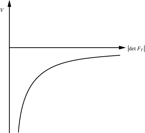
FIG. 1.: Sketch of the potential $V$ in Eq. (61).

It exhibits “fall to the origin” (like the classical hydrogen atom $s$-wave state) as already indicated by Eq. (59). Hence an additional ingredient seems required in the model. We will take the new ingredient to be a “non holomorphic” supersymmetry breaker. It will be required, as for the breaking terms in Eq. (39), to respect the full chiral group. For simplicity it will be treated as a perturbation in the sense that Eq. (54) and Eq. (60) will still be assumed to hold. In order not to disturb the matching conditions based on Eq. (46) we will assume the term to be scale invariant. A suitable form is

$$\delta V_{SB}=A\left(F^{*}F\right)^{r}\,\left[{\rm Tr}\left(F^{\dagger}_{T}F_{T}\right)\right]^{s}\ ,$$ (62)

where $A$ is a positive constant and $8r+6s=4$. For simplicity we will now consider the $N_{f}=1$ case. The results can be easily generalized to the case $N_{f}>1$. Using Eq. (60) for eliminating $|F|$ and substituting back into Eq. (62) we have

$$\delta V_{SB}=\frac{B}{|F_{T}|^{d}}\ ,$$ (63)

where the coefficients $B$ and $d$ are

$$B = A\left[\frac{\gamma}{N_{c}}\Lambda^{4+\frac{3}{p}}_{QCD}\left(\frac{\gamma}{N_{c}\tilde{\gamma}}\right)^{\frac{1}{p\tilde{\gamma}}}\right]^{2r}\ ,$$ (64)

$$d = \frac{1}{p}-s\left(\frac{3}{2p}+2\right).$$ (65)

The new potential, obtained by adding together Eq. (61) and Eq. (63) has a stable minimum when we choose $s<0$. The minimum condition also forces a non zero value for the quark-antiquark condensate $\langle F_{T}\rangle$ and no spontaneous breaking of strong CP symmetry ($\langle\Phi_{T}\rangle=0$). The generalization of this approach for $N_{f}>1$ would lead to a spontaneous breaking of chiral symmetry. It thus seems that a model of the present type, which includes “holomorphic” terms to satisfy the anomalies and supersymmetry breaking terms which include a “non holomorphic” piece can give a description of the properties of the QCD vacuum in general agreement with our expectations [29].

IV Discussion

We have shown that it is possible to construct toy models which explicitly realize the breaking of super gauge theories down to ordinary gauge theories in the effective Lagrangian framework. The resulting Lagrangians are built from the ordinary QCD glueball and meson fields. An important feature is the realization of the axial anomaly and the trace anomaly both at the supersymmetric as well as at the ordinary levels. The price we have paid for getting explicit results far away from the supersymmetric situation is the introduction of supersymmetry breaking terms chosen especially to simplify the calculation, while preserving the required symmetry properties.

For orientation we first studied the supersymmetric Yang Mills theory (described by the VY Lagrangian) and its breaking to ordinary Yang Mills. We learned, perhaps somewhat surprisingly, that both the decoupling of the gluino in the underlying theory as well as the expected nature of the Yang Mills vacuum could be understood with the neglect of the original Kähler terms. Our procedure led to a non supersymmetric potential (Eq. (18)) which possessed a kind of tree-level holomorphicity. It would be interesting to systematically investigate non holomorphic corrections due to the Kähler terms.

We next investigated the breaking of supersymmetric QCD (described by the TVY Lagrangian) down to ordinary QCD. Following a procedure similar to the previous one led to a plausible model for QCD which was consistent with the spontaneous breakdown of chiral symmetry and the generation of an $\eta^{\prime}$ mass ($U_{A}(1)$ problem). In this more complicated case the holomorphic piece of the potential, Eq. (53) had some nice features but gave a vacuum energy (see Fig. 1) unbounded from below. This was cured by the addition of a suitable non holomorphic piece, Eq. (62). For the QCD situation, both the Kähler terms as well as a supersymmetry breaking term like in Eq. (34) can give non holomorphic corrections. These should be investigated in more detail.

Of course, it would be fascinating to study more exotic situations using the present approach. In particular one can climb up Seiberg’s flavor ladder [1] encountering $N_{f}=N_{c}$ with baryonic composite fields and for $N_{f}>N_{c}$ eventually encountering non-Abelian dualities. Breaking $N=2$ supersymmetric gauge theories down to $N=1$ and ordinary gauge theories is clearly also of great interest.

A The $\theta$ dependence

Here we discuss the $\theta$ dependence of the potential Eq. (26), which represents a model in which the super-partners have been integrated out of the VY Lagrangian. To get an indication, which should be accurate for small $\hat{\theta}$, of what is happening we eliminate ${\rm Im}F$ from Eq. (26) by solving $\displaystyle{\frac{\partial V}{\partial{\rm Im}F}=0}$ to yield

$$\Phi=\frac{\gamma\hat{\theta}}{N_{c}}\ ,$$ (A1)

where $\Phi$ is defined from $F=-|F|e^{i\Phi}$. Substituting Eq. (A1) back into Eq. (26) together with ${\rm Im}F=\tan\Phi\,{\rm Re}F$ gives

$$V=-\frac{2N_{c}}{\gamma}{\rm Re}F\,\rm{ln}\,\left[\frac{N_{c}}{e\gamma\Lambda^{4}_{YM}}\frac{|{\rm Re}F|}{|\cos\left(\frac{\gamma\hat{\theta}}{N_{c}}\right)|}\right]\ .$$ (A2)

This has a minimum at

$$\langle|{\rm Re}F|\rangle=\frac{\gamma\Lambda^{4}_{YM}}{N_{c}}\left|\cos\left[\frac{\gamma}{N_{c}}\left(\theta+2\pi k\right)\right]\right|\ .$$ (A3)

At the minimum $\displaystyle{\langle V\rangle=-\frac{2N_{c}}{\gamma}\langle|{\rm Re}F|\rangle}$. Thus if $\theta$ is very small the global minimum will occur for $k=0$, if $\theta=2\pi+$ (very small) the global minimum will occur for $k=-1$, etc. In this way the $N_{c}-$fold degeneracy of the super Yang-Mills theory is broken.

In order to give a more accurate treatment when $\hat{\theta}$ is large, we may recognize that the mass diagonal (evaluated at the critical point of $V$) states are ${\rm Re}F^{\prime}$ and ${\rm Im}F^{\prime}$ where

$$F^{\prime}=e^{-i\frac{\gamma\hat{\theta}}{2N_{c}}}F\ .$$ (A4)

${\rm Im}F^{\prime}$ has negative squared mass and should, according to our earlier discussion, be integrated out from $\displaystyle{\frac{\partial V}{\partial({\rm Im}F^{\prime})}=0}$. This has the consequence

$$2\tan\left(\frac{\gamma\hat{\theta}}{2N_{c}}\right)\left[l-\rm{ln}\cos\Phi^{\prime}\right]+2\Phi^{\prime}-\frac{\gamma\hat{\theta}}{N_{c}}=0$$ (A5)

where $\displaystyle{l=\rm{ln}\,\left(\frac{N_{c}|{\rm Re}F^{\prime}|}{\gamma\Lambda^{4}_{YM}}\right)}$ and $\displaystyle{F^{\prime}=-|F^{\prime}|e^{i\Phi^{\prime}}}$. We may solve for $\Phi^{\prime}$ as a power series in $\hat{\theta}$:

$$\Phi^{\prime}=a\,\hat{\theta}+b\,\hat{\theta}^{2}+c\,\hat{\theta}^{3}+\cdots\ ,$$ (A6)

with $\displaystyle{a=\frac{\gamma}{2N_{c}}\left(1-l\right)}$, $b=0$, and $\displaystyle{c=-\frac{1}{2}\left(\frac{\gamma}{2N_{c}}\right)^{3}\left(1-\frac{4}{3}l+l^{2}\right)}$. Equation (A6) may be substituted back into $V$ and ${\rm Im}F^{\prime}=\tan\Phi^{\prime}\,{\rm Re}F^{\prime}$ eliminated. Correct to first order in $\hat{\theta}$ we get

$$V=+\frac{2N_{c}}{\gamma}|{\rm Re}F^{\prime}|\,\rm{ln}\,\left(\frac{N_{c}|{\rm Re}F^{\prime}|}{e\gamma\Lambda^{4}_{YM}}\right)+\rm{order}\left(\hat{\theta}^{2}\right)\ ,$$ (A7)

which is in agreement with Eq. (A2).

B Symmetries of Super QCD

At the classical level and in absence of the matter field mass terms, the global symmetry group for supersymmetric QCD is

$$G=SU_{L}(N_{f})\otimes SU_{R}(N_{f})\otimes U_{V}(1)\otimes U_{A}(1)\otimes\hat{U}_{R}(1)\ .$$ (B1)

The presence of the extra axial $R$ symmetry with respect to QCD is related to the gluino. At the superfield level the axial transformations are:

$$U_{A}(1):\qquad W^{\alpha}_{a}\rightarrow W^{\alpha}_{a},\qquad Q\rightarrow e^{i\alpha}Q,\qquad\tilde{Q}\rightarrow e^{i\alpha}\tilde{Q}\ .$$ (B2)

This symmetry is broken at the quantum level by the color Adler-Bell-Jackiw anomaly and the anomalous variation of the lagrangian is

$$\delta_{U_{A}(1)}{\cal L}=N_{f}\alpha\left(\frac{g^{2}}{32\pi^{2}}\epsilon_{mnrs}F^{mn}_{a}F^{rs}_{a}\right)\ .$$ (B3)

The $\hat{U}_{R}(1)$ transformation may be chosen as follows:

$$\hat{U}_{R}(1): W\left(x,\theta\right)\rightarrow e^{i\alpha\frac{3}{2}}W\left(x,e^{-i\alpha\frac{3}{2}}\theta\right)\ ,$$ (B4)

$${}Q\left(x,\theta\right)\rightarrow e^{i\alpha}Q\left(x,e^{-i\alpha\frac{3}{2}}\theta\right)\ ,$$ (B5)

$${\rm same~{}for~{}} \tilde{Q}\ .$$ (B6)

The anomalous variation of the fundamental lagrangian is

$$\delta_{\hat{U}_{R}(1)}{\cal L}=\left(3N_{c}-N_{f}\right)\alpha\left(\frac{g^{2}}{64\pi^{2}}\epsilon_{mnrs}F^{mn}_{a}F^{rs}_{a}\right)\ .$$ (B7)

It is possible to build an anomaly free transformation ${U}_{R}(1)$ which is a combination of the two previous anomalous $U(1)$’s:

$${U}_{R}(1): W\left(x,\theta\right)\rightarrow e^{-i\alpha N_{f}}W\left(x,e^{i\alpha N_{f}}\theta\right)\ ,$$ (B8)

$${}Q\left(x,\theta\right)\rightarrow e^{-i\alpha\left(N_{f}-N_{c}\right)}Q\left(x,e^{i\alpha N_{f}}\theta\right)\ ,$$ (B9)

$${\rm same~{}for~{}} \tilde{Q}\ .$$ (B10)

In Table I we summarize the axial charges of the relevant elementary and composite fields

Field	$U_{A}(1)$	$\hat{U}_{R}(1)$	${U}_{R}(1)$
$\lambda$	$0$	$+\frac{3}{2}$	$-N_{f}$
$\psi_{Q},~{}\psi_{\tilde{Q}}$	$+1$	$-\frac{1}{2}$	$N_{c}$
$\phi_{Q},~{}\phi_{\tilde{Q}}$	$+1$	$+1$	$N_{c}-N_{f}$
$S_{\theta=0}=\phi$	$0$	$+3$	$-2N_{f}$
$S_{\theta^{2}}=F$	$0$	$0$	$0$
$T_{\theta=0}=t$	$+2$	$+2$	$2\left(N_{c}-N_{f}\right)$
$T_{\theta^{2}}=F_{T}$	$+2$	$-1$	$2N_{c}$

TABLE I.: Axial charges for the relevant elementary and composite fields.

REFERENCES

- [1] N. Seiberg, Phys. Rev. D 49, 6857 (1994). N. Seiberg, Nucl. Phys. B435, 129 (1995).
- [2] N. Seiberg and E. Witten, Nucl. Phys. B426, 19 (1994), E 430, 495(1994); B431, 484 (1994).
- [3] K. Intriligator and N. Seiberg, Nucl. Phys. Proc. Suppl. 45BC, 1, 1996.
- [4] M.E. Peskin, Duality in Supersymmetric Yang-Mills Theory, (TASI 96): Fields, Strings, and Duality, Boulder, CO, 2-28 Jun 1996, hep-th/9702094.
- [5] P. Di Vecchia, Duality in Supersymmetric Gauge Theories, Surveys High Energy Phys. 10, 119 (1997), hep-th/9608090.
- [6] G. Veneziano and S. Yankielowicz, Phys. Lett. 113B, 321 (1982).
- [7] T.R. Taylor, G. Veneziano and S. Yankielowicz, Nucl. Phys. B218, 493 (1983).
- [8] I. Affleck, M. Dine and N. Seiberg, Nucl. Phys. B241, 493 (1984); B256, 557 (1985).
- [9] D. Amati, K. Konishi, Y. Meurice, G.C. Rossi and G. Veneziano, Phys. Rep. 162, 169 (1988).
- [10] V. Novikov, M. Shifman, A. Vainshtein and V. Zakharov, Nucl. Phys. B260, 157 (1985).
- [11] A. Masiero and G. Veneziano, Nucl. Phys. B249, 593 (1985).
- [12] A. Masiero, R. Pettorino, M. Roncadelli and G. Veneziano, Nucl. Phys. B261, 633 (1985).
- [13] O. Aharony, J. Sonnenshein, M. E. Peskin, and S. Yankielowicz, Phys, Rev. D 52, 6157 (1995).
- [14] N. Evans, S.D.H. Hsu and M. Schwetz, Phys. Lett. B 404, 77 (1997); Nucl. Phys. B484, 124 (1997); Lattice Tests of Supersymmetric Yang-Mills Theory, hep-th/9707260. N. Evans, S.D.H. Hsu, M. Schwetz, S.B. Selipsky, Nucl. Phys. B456, 205 (1995).
- [15] L. Alvarez-Gaume and M. Marino, Int. J. Mod. Phys. A12, 975 (1997). L. Alvarez-Gaume, J. Distler, C. Kounnas, M. Marino, Int. J. Mod. Phys. A11, 4745 (1996). L. Alvarez-Gaume, M. Marino, F. Zamora, Softly Broken N=2 QCD with Massive Quark Hypermultiplets, hep-th/9703072 and hep-th/9707017.
- [16] T. De Grand, R.L. Jaffe, K. Johnson and J. Kiskis, Phys. Rev. D12, 2066 (1975). M. Shifman, A. Vainshtein and V. Zakharov, Nucl. Phys. B147, 385 (1979); B147, 448 (1979).
- [17] J. Wess and J. Bagger, Supersymmetry and Supergravity, Princeton University Press, 1992.
- [18] S. Weinberg, Physica A96, 327 (1979). J. Gasser and H. Leutwyler, Ann. Phys. (NY) 158, 142 (1984); Nucl. Phys. B250, 465 (1985). A recent review is given by Ulf-G. Meissner, Rep. Prog. Phys. 56, 903 (1993).
- [19] S. Ferrara and B. Zumino, Nucl. Phys. B87, 207 (1975).
- [20] E. Witten, Nucl. Phys. B202, 513 (1981).
- [21] A. Kovner and M. Shifman, Chirally Symmetric Phase of Supersymmetric Gluodynamics, hep-th/9702174.
- [22] E. Witten, Nucl. Phys. B104, 445 (1976); B122, 109 (1977). See also M. Shifman et al. in [16].
- [23] J. Schechter, Phys. Rev. D21, 3393 (1980).
- [24] C. Rosenzweig, J. Schechter and G. Trahern, Phys. Rev. D21, 3388 (1980). P. Di Vecchia and G. Veneziano, Nucl. Phys. B171, 253 (1980). E. Witten, Ann. of Phys. 128, 363 (1980). P. Nath and A. Arnowitt, Phys. Rev. D23, 473 (1981). A. Aurilia, Y. Takahashi and D. Townsend, Phys. Lett. 95B, 265 (1980). K. Kawarabayashi and N. Ohta, Nucl. Phys. B175, 477 (1980).
- [25] A.A. Migdal and M.A. Shifman, Phys. Lett. 114B, 445 (1982). J.M. Cornwall and A. Soni, Phys. Rev. D29, 1424 (1984); 32, 764 (1985).
- [26] A. Salomone, J. Schechter and T. Tudron, Phys. Rev. D23, 1143 (1981). J. Ellis and J. Lanik, Phys. Lett. 150B, 289 (1985). H. Gomm and J. Schechter, Phys. Lett. 158B, 449 (1985).
- [27] H. Gomm, P. Jain, R. Johnson and J. Schechter, Phys. Rev. D33, 801 (1986).
- [28] H. Gomm, P. Jain, R. Johnson and J. Schechter, Phys. Rev. D33, 3476 (1986).
- [29] Actually a QCD Lagrangian with a similar “holomorphic” piece plus a needed non holomorphic piece was discussed in sect. VII of Ref. [27]. This was partly motivated by a complex form for the two QCD coupling parameters which had been speculated in J. Schechter, Proceedings of the third annual MRST meeting, University of Rochester, April 30 - May 1 (1981).