osp$\bf{(1|2)}$ Conformal Field Theory

I.P. Ennes A.V. Ramallo and J. M. Sanchez de Santos

Departamento de Física de Partículas,

Universidad de Santiago

E-15706 Santiago de Compostela, Spain.

ABSTRACT

We review some results recently obtained for the conformal field theories based on the affine Lie superalgebra ${\rm osp}(1|2)$. In particular, we study the representation theory of the ${\rm osp}(1|2)$ current algebras and their character formulas. By means of a free field representation of the conformal blocks, we obtain the structure constants and the fusion rules of the model.
Lecture delivered at the CERN-Santiago de Compostela-La Plata Meeting, “Trends in Theoretical Physics”, La Plata, Argentina, April-May 1997.

US-FT-26/97 August 1997

hep-th/9708094

1 Introduction and motivation

Among the two-dimensional theories endowed with conformal invariance, those which, in addition, possess a current algebra symmetry are specially important [1]. In this lecture, we shall report on some results we have recently obtained for Conformal Fields Theories (CFT’s) which enjoy an ${\rm osp}(1|2)$ affine superalgebra. As a motivation for the study of this particular case, let us mention that the ${\rm osp}(1|2)$ super Lie algebra has an ubiquitous presence in many problems in which the $N=1$ superconformal symmetry is involved. Indeed, the minimal $N=1$ superconformal models can be obtained by means of Hamiltonian reduction of a system with ${\rm osp}(1|2)$ current algebra and this symmetry appears in the light-cone approach to two-dimensional supergravity [2, 3]. It is also interesting to mention in this respect that the topological ${\rm osp}(1|2)/{\rm osp}(1|2)$ coset theories can be used to describe the non-critical Ramond-Neveu-Schwarz superstrings [4, 5]. As a final motivation let us point out that, as will be shown below, a lot of non-trivial results can be found for the ${\rm osp}(1|2)$ CFT’s. These results can be simply stated and compared with those corresponding to CFT’s based on the su$(2)$ affine Lie algebra.

The organization of this lecture is the following. In section 2 we recall the basic facts of the ${\rm osp}(1|2)$ representation theory. Its similarity with ordinary angular momentum theory will become evident and will constitute a guiding principle for what follows. The ${\rm osp}(1|2)$ current algebra is introduced in section 3 and the corresponding character formulas are analyzed in section 4. In section 5 we study a representation of the affine ${\rm osp}(1|2)$ symmetry in terms of free fields. This representation can be used to give integral expressions for the conformal blocks, from which the structure constants and the fusion rules of the model can be extracted. Finally, in section 6 some conclusions are drawn and a series of final remarks are made.

2 osp$\bf{(1|2)}$ Representation Theory

The ${\rm osp}(1|2)$ superalgebra is a graded extension of the $sl(2)$ Lie algebra [6]. It is generated by three bosonic generators ($T_{3}$ and $T_{\pm}$ ) and by two fermionic operators ($F_{\pm}$). The bosonic generators close an $sl(2)$ algebra. The full set of (anti)commutators that define the ${\rm osp}(1|2)$ superalgebra is:

$$[T_{3}\,,\,T_{\pm}]\,=\,\pm T_{\pm}\,\,\,\,\,\,\,\,\,\,\,\,\,\,\,\,\,\,\,\,\,\,\,\,\,\,\,\,\,\,\,\,\,\,\,\,\,\,\,\,\,\,[T_{+}\,,\,T_{-}]\,=\,2T_{3}$$

$$[T_{3}\,,\,F_{\pm}]\,=\,\pm{1\over 2}F_{\pm}\,\,\,\,\,\,\,\,\,\,\,\,\,\,\,\,\,\,\,\,\,\,\,\,\,\,\,\,\,\,\,\,\,\,\,\,\,\{F_{\pm}\,,\,F_{\pm}\}\,=\,\pm 2T_{\pm}$$ (2.1)

$$\{F_{+}\,,\,F_{-}\}\,=\,2T_{3}\,\,\,\,\,\,\,\,\,\,\,\,\,\,\,\,\,\,\,\,\,\,\,\,\,\,\,\,\,\,\,\,\,\,\,\,\,\,\,\,\,\,[T_{\pm}\,,\,F_{\pm}]\,=\,0$$

$$[T_{\pm}\,,\,F_{\mp}]\,=\,-F_{\pm}\,\,.$$

It can be easily checked from (2.1) that the operator:

$$C_{2}\,=\,T_{3}^{2}\,+\,{1\over 2}\,[\,T_{-}T_{+}\,+\,T_{+}T_{-}\,]\,+\,{1\over 4}\,[\,F_{-}F_{+}\,-\,F_{+}F_{-}\,]\,,$$ (2.2)

commutes with all the generators of the ${\rm osp}(1|2)$ algebra. $C_{2}$ is the so-called quadratic Casimir operator. Using the algebra defining relations (eq. (2.1)) one can reexpress $C_{2}$ as:

$$C_{2}\,=\,T_{3}^{2}\,+\,{1\over 2}\,T_{3}\,+\,T_{-}T_{+}\,+\,{1\over 2}\,F_{-}F_{+}\,.$$ (2.3)

Following the standard methods of angular momentum theory, one can find matrix representations of the algebra (2.1). The finite dimensional irreducible representations ${\cal R}_{j}$ of the ${\rm osp}(1|2)$ theory are labeled by an integer or half-integer number $j$, which we shall refer to as the isospin of the representation. The highest weight vector of the representation ${\cal R}_{j}$ will be denoted by $|j,j>$. It satisfies the conditions:

$$T_{+}\,|j,j>\,=\,F_{+}\,|j,j>\,=\,0\,.$$ (2.4)

From the vector $|j,j>$, one can easily obtain other vectors of ${\cal R}_{j}$ by acting with the lowering operators $T_{-}$ and $F_{-}$. We shall denote by $|j,m>$ to a general basis state for the representation ${\cal R}_{j}$, $m$ being the $T_{3}$ eigenvalue. The quadratic Casimir operator $C_{2}$ acts on the states $|j,m>$ as a multiple of the identity operator. The precise action of $C_{2}$ on the states of ${\cal R}_{j}$ can be determined by computing $C_{2}\,|j,j>$ from the highest weight conditions (2.4). The result is:

$$C_{2}\,|j,m>\,=\,j\,(\,j+{1\over 2}\,)\,|j,m>\,.$$ (2.5)

It is not difficult to obtain the matrix elements of the generators of ${\rm osp}(1|2)$ in the representation ${\cal R}_{j}$. For the bosonic generators one has:

$$T_{3}\,|j,m>\,=\,m|j,m>$$

$$T_{\pm}\,|j,m>\,=\,\sqrt{\,[j\mp m]\,[j\pm m+1]}\,|j,m\pm 1>\,\,,$$ (2.6)

where $[x]$ represents the integer part of the number $x$ ($2x\in{\rm Z}\kern-3.8pt{\rm Z}\kern 2.0pt$). The action of the operators $F_{\pm}$ on the states $|j,m>$ is the following:

$$F_{\pm}\,|j,m>\,=\,\cases{-\sqrt{j\mp m}\,|j,m\pm{1\over 2}>&if $j-m\in{\rm Z}\kern-3.8pt{\rm Z}\kern 2.0pt$\cr\cr\mp\sqrt{j\pm m+{1\over 2}}\,|j,m\pm{1\over 2}>&if $j-m\in{\rm Z}\kern-3.8pt{\rm Z}\kern 2.0pt+{1\over 2}$.}$$ (2.7)

Notice that the operators $T_{\pm}$ ($F_{\pm}$) change the $T_{3}$ eigenvalue in $\pm 1$ ($\pm 1/2$). In addition, the fermionic operators change the statistics of the states. It is clear from (2.6) and (2.7) that, when $2j\in{\rm Z}\kern-3.8pt{\rm Z}\kern 2.0pt$, the representation ${\cal R}_{j}$ is $4j+1$-dimensional and spanned by the states $|j,m>$ with $m=-j,-j+{1\over 2},\cdots,j-{1\over 2},j$. In order to characterize completely the representation one must give the statistics of its highest weight state. The Grassmann parity of $|j,j>$ will be denoted by $p(j)$ ($p(j)=0,1$). We will say that the representation ${\cal R}_{j}$ is even(odd) when $|j,j>$ is bosonic(fermionic), i.e. when $p(j)=0$($p(j)=1$). It is clear that the Grassmann parity of the state $|j,m>$ is $p(j)+2(j-m)\,\,$ ${\rm mod}\,(2)$.

For Lie superalgebras, one can define a generalized adjoint operation, denoted by $\ddagger$, such that, for any operator $A$ and any two states $\alpha$ and $\beta$, one has:

$$<A^{\ddagger}\alpha|\beta>\,=\,(-1)^{p(A)p(\alpha)}\,\,<\alpha|A\beta>\,.$$ (2.8)

We shall call $A^{\ddagger}$ the superadjoint of $A$. In eq. (2.8), $p(A)$ and $p(\alpha)$ denote respectively the Grassmann parities of the operator $A$ and the state $\alpha$. One can verify that the superadjoint of the product of two operators is given by the formula:

$$(AB)^{\ddagger}\,=\,(-1)^{p(A)p(B)}\,\,B^{\ddagger}\,A^{\ddagger}\,\,.$$ (2.9)

It is easy to prove that the compatibility of the property (2.9) and the relations (2.1) requires that $T_{\pm}^{\,\ddagger}\,=\,T_{\mp}$ and $T_{3}^{\ddagger}\,=\,T_{3}$. In the case of the fermionic generators we have, however, some freedom. Actually, if $\eta$ is a number that can take the values $\pm 1$, the rule which makes the superadjoint $F_{\pm}^{\ddagger}$ consistent with the (anti)commutators (2.1) is:

$$F_{+}^{\ddagger}\,=\,\eta\,F_{-}\,\,\,\,\,\,\,\,\,\,\,\,\,\,\,\,\,\,\,\,\,F_{-}^{\ddagger}\,=\,-\eta\,F_{+}\,\,.$$ (2.10)

It is important to point out that, in any case, $(\,(\,F_{\pm}\,)^{\ddagger}\,)^{\ddagger}\,=\,-F_{\pm}$. The value of $\eta$ is related to the norm of the states and the parity $p(j)$ of the representation. To illustrate this point let us suppose that $<j,m|j,m>\,=\,\epsilon(\epsilon^{\prime})$ if $j=m$ is integer(half-integer), where $\epsilon$ and $\epsilon^{\prime}$ can take the value $+1$ or $-1$. Putting in eq. (2.8) $\alpha\,=\,|j,j>$, $\beta\,=\,|j,j-{1\over 2}>$ and $A\,=\,F_{+}$, one gets:

$$\eta\,=\,(-1)^{p(j)}\,\epsilon\epsilon\,^{\prime}\,\,.$$ (2.11)

Once we conventionally fix $\eta$ to a given value, the signs $\epsilon$ and $\epsilon^{\prime}$ of the norms of the states are related to the highest weight parity $p(j)$ by means of eq. (2.11). For simplicity, we shall choose $\eta=1$, which implies that $\epsilon\epsilon\,^{\prime}\,=\,(-1)^{p(j)}$. For even representations, $p(j)=0$ and the norms $\epsilon$ and $\epsilon\,^{\prime}$ can be taken to be $+1$, whereas for odd representations, $\epsilon$ and $\epsilon\,^{\prime}$ must have opposite sign. We shall choose $\epsilon\,=\,-\epsilon\,^{\prime}\,=\,+1$ for odd representations and, therefore, the norms of the states will be given by the expression:

$$<j,m|j,m>\,=\,(-)^{2p(j)(j-m)}\,\,.$$ (2.12)

When two representations of isospins $j_{1}$ and $j_{2}$ are coupled, one can decompose the corresponding tensor product in the following way:

$${\cal R}_{j_{1}}\,\otimes{\cal R}_{j_{2}}\,=\,\bigoplus_{{j_{3}=|j_{1}-j_{2}|\atop}\atop 2(j_{3}-j_{1}-j_{2})\,\in\,{\rm Z}\kern-3.8pt{\rm Z}\kern 2.0pt}^{j_{1}+j_{2}}\,{\cal R}_{j_{3}}\,\,,$$ (2.13)

which means that one gets representations of isospins $|j_{1}-j_{2}|\,,\,|j_{1}-j_{2}|+{1\over 2}\,,\cdots,j_{1}+j_{2}-{1\over 2}\,,\,j_{1}+j_{2}$. The parity of the representation ${\cal R}_{j_{3}}$ in the right-hand side of eq. (2.13) is given by:

$$p(j_{3})\,=\,p(j_{1})\,+\,p(j_{2})\,+\,2(j_{1}+j_{2}-j_{3})\,\,\,\,\,\,\,\,\,\,\,\,\,\,\,\,\,\,\,\,{\rm mod}\,(2)\,\,.$$ (2.14)

Notice that eq. (2.14) implies that odd representations appear when even representations are coupled. In fact, if we denote by $[j]$ and $\widetilde{[j]}$ to the even and odd representations of isospin $j$, eqs. (2.13) and (2.14) imply, in particular, that:

$$[{\scriptstyle{1\over 2}}]\,\otimes[{\scriptstyle{1\over 2}}]\,= \,[0]+\widetilde{[{\scriptstyle{1\over 2}}]}+[1]\,$$

$$\,[1]\,\otimes\,[1]\,= \,[0]+\widetilde{[{\scriptstyle{1\over 2}}]}+[1]+\widetilde{[{\scriptstyle{3\over 2}}]}+[2]\,\,.$$ (2.15)

The presence of odd representations in the right-hand side of eq. (2.15) means that one cannot avoid having negative norm states and, therefore, a theory enjoying this symmetry cannot be unitary.

3 osp$\bf{(1|2)}$ Current Algebra

In order to construct a Conformal Field Theory endowed with the ${\rm osp}(1|2)$ symmetry, one must first extend the finite algebra of section 2 to the affine, infinite dimensional, ${\rm osp}(1|2)$ Lie superalgebra. As it is well-known, this can be achieved by replacing the generators of section 2 by currents depending on a holomorphic variable $z$:

$$T_{\pm}\,\,\Longrightarrow\,\,J^{\pm}(z)\,=\,\sum_{n=-\infty}^{+\infty}J^{\pm}_{n}\,z^{-n-1}$$

$$T_{3}\,\,\Longrightarrow\,\,J^{0}(z)\,=\,\sum_{n=-\infty}^{+\infty}J^{0}_{n}\,z^{-n-1}$$ (3.1)

$$F_{\pm}\,\,\Longrightarrow\,\,j^{\pm}(z)\,=\,\sum_{n=-\infty}^{+\infty}\,\,j^{\pm}_{n}\,z^{-n-1}\,\,.$$

In eq. (3.1), we have displayed the mode expansions of the different currents. Notice that the modes $n$ of the fermionic currents run over the integers, which implies that we are considering the Ramond sector of the ${\rm osp}(1|2)$ affine superalgebra. The non-vanishing (anti)commutators of the currents $J_{n}^{a}$ and $j_{n}^{\alpha}$ are:

$$[\,J_{n}^{0}\,,\,J_{m}^{\pm}\,]\,=\,\pm J_{n+m}^{\pm}\,\,\,\,\,\,\,\,\,\,\,\,\,\,\,\,\,\,\,\,\,\,\,\,\,\,\,\,\,\,\,\,\,\,\,\,\,\,\,\,\,\,\,\,\,\,\,\,\,\,[\,J_{n}^{0}\,,\,J_{m}^{0}\,]\,=\,{k\over 2}\,n\,\delta_{n+m}$$

$$[\,J_{n}^{+}\,,\,J_{m}^{-}\,]\,=\,kn\delta_{n+m}\,+\,2J^{0}_{n+m}$$

$$[\,J_{n}^{0}\,,\,j_{m}^{\pm}\,]\,=\,\pm\,{1\over 2}\,j_{m+n}^{\pm}\,\,\,\,\,\,\,\,\,\,\,\,\,\,\,\,\,\,\,\,\,\,\,\,\,\,\,\,\,\,\,\,\,\,\,\,\,\,\,\,\,\,\,\,\,[\,J_{n}^{\pm}\,,\,j_{m}^{\pm}\,]\,=\,0$$ (3.2)

$$[\,J_{n}^{\pm}\,,\,j_{m}^{\mp}\,]\,=\,-j_{n+m}^{\pm}\,\,\,\,\,\,\,\,\,\,\,\,\,\,\,\,\,\,\,\,\,\,\,\,\,\,\,\,\,\,\,\,\,\,\,\,\,\,\,\,\,\,\,\,\,\,\,\,\,\,\{\,j_{n}^{\pm}\,,\,j_{m}^{\pm}\,\}\,=\,\pm 2J_{n+m}^{\pm}$$

$$\{\,j_{n}^{+}\,,\,j_{m}^{-}\,\}\,=\,2kn\delta_{n+m}\,+\,2J^{0}_{n+m}\,\,.$$

In what follows, the algebra defined in (3.2) will be simply denoted by ${\cal A}$. By inspecting eq. (3.2), one can verify that the zero modes $J_{0}^{a}$ and $j_{0}^{\alpha}$ of the currents close the algebra (2.1). In eq. (3.2), $k$ is a central element (the level of the ${\rm osp}(1|2)$ current algebra) which commutes with all the other generators. By means of the Sugawara prescription, one can construct an energy-momentum tensor $T(z)$ for the ${\rm osp}(1|2)$ currents. The expression of $T(z)$ is the following:

$$T(z)\,=\,{1\over 2k+3}\,:\,[\, 2\,(J^{0}(z))^{2}\,+\,J^{+}(z)\,J^{-}(z)\,+\,J^{-}(z)\,J^{+}(z)\,-$$ (3.3)

$$-\,{1\over 2}\,j^{+}(z)\,j^{-}(z)\,+\,{1\over 2}\,j^{-}(z)\,j^{+}(z)\,]:\,\,,$$

where the double dot $:$ denotes normal ordering. The modes $L_{n}$ of the energy-momentum tensor are defined as:

$$T(z)\,=\,\sum_{n=-\infty}^{+\infty}\,\,L_{n}\,z^{-n-2}\,\,.$$ (3.4)

A calculation performed with the standard techniques of CFT allows to prove that the commutators of the $L_{n}$’s with the currents are:

$$[\,L_{n}\,,\,J_{m}^{a}\,]\,=\,-m\,J_{n+m}^{a}\,\,\,\,\,\,\,\,\,\,\,\,\,\,\,\,\,\,\,\,[\,L_{n}\,,\,j_{m}^{\alpha}\,]\,=\,-m\,j_{n+m}^{\alpha}\,\,.$$ (3.5)

Similarly, one can verify that the modes of the energy-momentum tensor satisfy the Virasoro algebra:

$$[\,L_{n},L_{m}\,]\,=\,(n-m)\,L_{n+m}\,+\,{c\over 12}\,\,(m^{3}\,-\,m)\,\delta_{n+m,0}\,\,,$$ (3.6)

where the central charge $c$ is related to the level $k$ by means of the expression:

$$c\,=\,{2k\over 2k+3}\,\,.$$ (3.7)

In the algebra (3.2), we can introduce the so-called principal gradation, which is defined as:

$$d(\,J_{n}^{a}\,)\,=\,2n\,+\,a\,\,\,\,\,\,\,\,\,\,\,\,\,\,\,d(\,j_{n}^{\alpha}\,)\,=\,2n\,+\,{\alpha\over 2}\,\,\,\,\,\,\,\,\,\,\,\,\,\,\,d(\,k\,)\,=\,0\,\,.$$ (3.8)

With respect to $d$, the algebra ${\cal A}$ splits as:

$${\cal A}\,=\,{\cal A}_{-}\,\oplus\,{\cal A}_{0}\,\oplus\,{\cal A}_{+}\,\,,$$ (3.9)

where ${\cal A}_{-}$, ${\cal A}_{0}$ and ${\cal A}_{+}$ are the subspaces of ${\cal A}$ spanned by the elements that have, respectively, $d<0$, $d=0$ and $d>0$. These elements are easy to identify from eq. (3.8) and so, for example, ${\cal A}_{0}$ is generated by $J_{0}^{0}$ and $k$, whereas ${\cal A}_{+}$ is the subspace spanned by $J_{n}^{-}\,\,(n\geq 1)$, $J_{n}^{0}\,\,(n\geq 1)$, $J_{n}^{+}\,\,(n\geq 0)$, $j_{n}^{-}\,\,(n\geq 1)$ and $j_{n}^{+}\,\,(n\geq 0)$.

The Verma modules associated to ${\cal A}$ are constructed by acting with elements of the universal enveloping algebra of ${\cal A}_{-}$ (denoted by $U(\,{\cal A}_{-}\,)$) on a highest weight vector $|\,j,k>$. The latter is annihilated by the elements of ${\cal A}_{+}$, i.e.:

$$J_{n}^{a}\,|\,j,k>\,=\,j_{n}^{\alpha}\,|\,j,k>\,=\,0\,\,,\,\,\,\,\,\,\,\,\,\,\,\,\,\,\,\,\,\,\forall\,\,(\,J_{n}^{a}\,,\,j_{n}^{\alpha}\,)\,\in\,{\cal A}_{+}\,\,.$$ (3.10)

On the contrary, $J_{0}^{0}$ and $L_{0}$ act diagonally on $|\,j,k>$:

$$J_{0}^{0}\,|\,j,k>\,=\,j\,|\,j,k>\,\,\,\,\,\,\,\,\,\,\,\,\,\,\,\,\,\,L_{0}\,|\,j,k>\,=\,h_{j}\,|\,j,k>\,\,.$$ (3.11)

From the Sugawara expression for $L_{0}$ (see eqs. (3.3) and (3.4) ), one can easily get the $L_{0}$ eigenvalue corresponding to $|\,j,k>$, namely:

$$h_{j}\,=\,{j\,(\,2j\,+\,1\,)\over 2k\,+\,3}\,\,.$$ (3.12)

As in the case of the finite algebra, in order to characterize completely the highest weight vector $|\,j,k>$, we must specify its Grassmann parity, which we shall also denote by $p(j)$. The Verma module whose highest weight vector is $|\,j,k>$ will be denoted by $V^{(j,k)}$. Any element in $V^{(j,k)}$ is of the form $u_{-}|\,j,k>$, where $u_{-}\in{\cal A}_{-}$. Notice that, according to the Poincaré-Birkhoff-Witt theorem, $U(\,{\cal A}_{-}\,)$ is generated by monomials and thus we can consider a basis of $V^{(j,k)}$ constituted by vectors of the form:

$${|\,\{m_{i}^{a}\}\,;j\,>}\,=\,\prod_{i=0}^{+\infty}\,\Bigl{(}\,j_{-i}^{-}\,\Bigr{)}^{2m_{i}^{-}}\,\,\prod_{i=1}^{+\infty}\,\Bigl{(}\,J_{-i}^{0}\,\Bigr{)}^{m_{i}^{0}}\,\,\prod_{i=1}^{+\infty}\,\Bigl{(}\,j_{-i}^{+}\,\Bigr{)}^{2m_{i}^{+}}\,\,|\,j,k>\,\,.$$ (3.13)

In eq. (3.13), the numbers $m_{i}^{\pm}$ are integers or half-integers whereas the $m_{i}^{0}$’s are always integers ($m_{i}^{a}\geq 0$).

For some values of the isospin $j$ the Verma module $V^{(j,k)}$ is reducible, i.e. it contains singular vectors. These are vectors of $V^{(j,k)}$ which are descendants and are annihilated by ${\cal A}_{+}$. For a given value of the level $k$, the singular vectors appear in those modules with highest weight vectors whose isospins belong to a discrete set labelled by two integers $r$ and $s$. These isospins are of the form [7]:

$$4j_{r,s}\,+\,1\,=\,r\,-\,s\,(\,2k+3\,)\,\,,$$ (3.14)

where $r+s$ is odd and, either $r>0$ and $s\geq 0$ or $r<0$ and $s<0$. The $J_{0}^{0}$ and $L_{0}$ eigenvalues of these vectors are respectively $j_{r,s}\,-{r\over 2}$ and $h_{j_{r,s}}\,+\,{rs\over 2}$.

4 osp$\bf{(1|2)}$ character formulae

Let us now study the characters of the ${\rm osp}(1|2)$ CFT. For an irreducible Verma module $V^{(j,k)}$, whose highest weight vector has isospin $j$, the characters $\lambda_{j}(a,\tau)$ are defined as:

$$\lambda_{j}(a,\tau)\,=\,{\rm Tr}_{j}\,[\,q^{L_{0}-{c\over 24}}\,w^{J_{0}^{0}}\,]\,,$$ (4.1)

where the trace is taken over the module $V^{(j,k)}$ and $q$ and $w$ are two variables related to the modular parameter $\tau$ and to the Cartan coordinate $a$ by means of the expressions:

$$q\,=\,e^{2\pi i\tau}\,\,\,\,\,\,\,\,\,\,\,\,\,\,\,\,\,\,\,\,w\,=\,e^{2\pi ia}\,\,.$$ (4.2)

The trace in eq. (4.1) can be evaluated by studying the action of the operator $q^{L_{0}-{c\over 24}}\,w^{J_{0}^{0}}$ on the states $|\,\{m_{i}^{a}\}\,;j\,>$ defined in eq. (3.13). Since $L_{0}$ and $J_{0}^{0}$ act diagonally on these states, the trace (4.1) can be easily calculated. After some simple manipulations [7, 8], one obtains the following expression for $\lambda_{j}(a,\tau)$:

$$\lambda_{j}(a,\tau)\,=\,{q^{{2(j\,+{1\over 4})^{2}\over 2k\,+\,3}}\,w^{j+\,{1\over 4}}\over\Pi(a,\tau)}\,,$$ (4.3)

where the function $\Pi(a,\tau)$, appearing in the denominator, is the following infinite product:

$$\Pi(a,\tau)\,\equiv\,q^{{1\over 24}}\,w^{{1\over 4}}\,\prod_{n=1}^{+\infty}\,\,(1-q^{n})\,(1-w^{{1\over 2}}q^{n})\,(1-w^{-{1\over 2}}q^{n-1})\,(1-wq^{2n-1})\,(1-w^{-1}q^{2n-1})\,.$$ (4.4)

By means of the Watson quintuple product identity:

$$\prod_{n=1}^{+\infty}\,\, (1-q^{n})\,(1-wq^{n})\,(1-w^{-1}q^{n-1})\,(1-w^{2}q^{2n-1})\,(1-w^{-2}q^{2n-1})\,=\,$$ (4.5)

$$=\,\sum_{m=-\infty}^{+\infty}\,\,(w^{3m}-w^{-3m-1})\,q^{{3m^{2}+m\over 2}}\,\,,$$

one can write $\Pi(a,\tau)$ in the form:

$$\Pi(a,\tau)\,=\,\Theta_{1,3}\,({a\over 2},{\tau\over 2})\,-\,\Theta_{-1,3}\,({a\over 2},{\tau\over 2})\,\,,$$ (4.6)

where $\Theta_{r,s}$ are the classical theta functions, defined as:

$$\Theta_{r,s}\,(a,\tau)\,=\,\sum_{m\in{\rm Z}\kern-3.8pt{\rm Z}\kern 2.0pt}\,q^{s(m+{r\over 2s})^{2}}\,w^{s(m+{r\over 2s})}\,.$$ (4.7)

For some particular values of the level $k$ there exists a class of representations which are completely degenerate [7, 8]. These representations occur for values of $k$ which are rational numbers of the form:

$$2k+3\,=\,{p\over p^{\prime}}\,\,,$$ (4.8)

where $p$ and $p^{\prime}$ are coprime positive integers such that $p+p^{\prime}$ is even and $p$ and $(p+p^{\prime})/2$ are relatively prime. The so-called admissible representations correspond to isospins of the form:

$$4j_{r,s}\,+\,1\,=\,r\,-\,s\,{p\over p\,^{\prime}}\,\,,$$ (4.9)

with $r$ and $s$ taking values in the grid $1\leq r\leq p-1$, $0\leq s\leq p^{\prime}-1$ and $r+s\in 2{\rm Z}\kern-3.8pt{\rm Z}\kern 2.0pt+1$. When the isospin is of the form (4.9), the corresponding Verma module will have a null vector, since eq. (4.9) corresponds to eq. (3.14) with $r>0$ and $s\geq 0$. Moreover, when eqs. (4.8) and (4.9) are satisfied, one has that $j_{r,s}\,=\,j_{r-p,s-p^{\prime}}$ and, therefore, when $r$ and $s$ belong to the grid defined above, the isospin (4.9) has also the form (3.14) for the integers $r-p<0$ and $s-p^{\prime}<0$. Therefore, when the isospin $j_{r,s}$ belongs to the admissible set (4.9), the module $V^{j_{r,s},k}$ possesses a second singular vector. These two null vectors generate the maximum proper submodule of $V^{j_{r,s},k}$, which can be generated by means of the embedding diagram:

$$\matrix{&&B(0)&\longrightarrow&B(1)&\longrightarrow&B(1)&\longrightarrow&A(2)&\longrightarrow&\cdots\cr A(0)&\nearrow\atop\searrow&&\nearrow\!\!\!\!\!\!\searrow&&\nearrow\!\!\!\!\!\!\searrow&&\nearrow\!\!\!\!\!\!\searrow&&\nearrow\!\!\!\!\!\!\searrow&\cdots\cr&&B(-1)&\longrightarrow&A(-1)&\longrightarrow&B(-2)&\longrightarrow&A(-2)&\longrightarrow&\cdots\cr}$$

where $A(l)$ and $B(l)$ are given by:

$$A(l)\, \equiv\,j_{r-2lp\,,\,s}\,=\,{r-1\over 4}\,-\,{s\over 4}\,{p\over p\,^{\prime}}\,-\,l\,{p\over 2}$$

$$B(l)\, \equiv\,j_{-r-2lp\,,\,s}\,=\,{r-1\over 4}\,-\,{s\over 4}\,{p\over p\,^{\prime}}\,-\,l\,{p\over 2}\,-\,{r\over 2}\,\,.$$ (4.10)

Each node in the above diagram represents a Verma module with $A(l)$ or $B(l)$ as the isospin of its highest weight state. An arrow connecting two spaces $E\rightarrow F$ means that the module $F$ is contained in the module $E$. The character of the irreducible module with isospin $j=j_{r,s}$ is constructed as an alternating sum of the form:

$$\chi_{j_{r,s}}(a,\tau)\,=\,\sum_{l=-\infty}^{l=+\infty}\,\,\lambda_{A(l)}(a,\tau)\,-\,\sum_{l=-\infty}^{l=+\infty}\,\,\lambda_{B(l)}(a,\tau)\,\,.$$ (4.11)

Using eqs. (4.3) and (4.10) in the right-hand side of eq. (4.11), it is straightforward to prove that $\chi_{j_{r,s}}(a,\tau)$ can be written as a quotient of differences of theta functions. Actually, defining the constants $b_{\pm}$ and $e$ as:

$$b_{\pm}\,=\,\pm p\,^{\prime}r\,-\,p\,s\,\,\,\,\,\,\,\,\,\,\,\,\,\,\,\,\,\,\,\,\,\,\,\,\,e\,=\,p\,p\,^{\prime}\,\,,$$ (4.12)

the characters $\chi_{j_{r,s}}(a,\tau)$ can be put in the form:

$$\chi_{j_{r,s}}(a,\tau)\,=\,{\Theta_{b_{+},e}({a\over 2p\,^{\prime}},{\tau\over 2}\,)\,-\,\Theta_{b_{-},e}({a\over 2p\,^{\prime}},{\tau\over 2}\,)\over\Pi(a,\tau)}\,\,.$$ (4.13)

It is interesting to study the behaviour of the characters (4.13) when $a\rightarrow 0$ [9]. First of all, it is easy to prove that the denominator $\Pi(a,\tau)$ vanishes linearly when $a\rightarrow 0$. Actually, one can check that:

$$\Pi(a,\tau)\,=\,i\pi aq^{{1\over 24}}\,\sum_{m\in{\rm Z}\kern-3.8pt{\rm Z}\kern 2.0pt}\,(6m+1)\,q^{{3m^{2}+m\over 2}}\,+\,o(a^{2})\,\,.$$ (4.14)

In general, the numerator of the right-hand side of eq. (4.13) does not vanish when $a=0$. Therefore $\chi_{j_{r,s}}(a,\tau)$ will, in general, develop a single pole in $a$ in the $a\rightarrow 0$ limit. By studying the residue of the ${\rm osp}(1|2)$ characters in this singularity we are going to discover a remarkable connection with the minimal supersymmetric models. Let us, first of all, rewrite the infinite sum appearing in the right-hand side of eq. (4.14) as an infinite product. An identity due to Gordon [10] states that:

$$q^{{1\over 24}}\,\sum_{m\in{\rm Z}\kern-3.8pt{\rm Z}\kern 2.0pt}\,(6m+1)\,q^{{3m^{2}+m\over 2}}\,=\,2\,{\Big{[}\,\eta(\tau)\,\Big{]}^{4}\over\theta_{2}(0,\tau)}\,\,,$$ (4.15)

where $\eta(\tau)$ is the Dedekind $\eta$-function, which can be represented as:

$$\eta(\tau)\,=\,q^{{1\over 24}}\,\prod_{n=1}^{\infty}\,(1\,-\,q^{n})\,\,.$$ (4.16)

and $\theta_{2}(0,\tau)$ is a Jacobi theta function, whose infinite product representation can be obtained from (4.16) and from the following relation with $\eta(\tau)$:

$${\theta_{2}(0,\tau)\over\eta(\tau)}\,=\,2\,q^{{1\over 12}}\,\prod_{n=1}^{\infty}\,(\,1\,+\,q^{n}\,)^{2}\,\,.$$ (4.17)

It is easy to verify that the numerator of the ${\rm osp}(1|2)$ characters does not vanish when $s\not=0$ (see eq. (4.13)). Therefore, it makes sense to consider the residue of $\chi_{j_{r,s}}(a,\tau)$ at the point $a=0$. Let us define for $s\not=0$ the following quantity:

$$\hat{\chi}_{r,s}(\tau)\,\equiv\,\Big{[}\,{2\eta(\tau)\over\theta_{2}(0,\tau)}\,\Big{]}^{1\over 2}\,\,\Big{[}\,\eta(\tau)\,\Big{]}^{2}\,\,{\rm lim}_{a\rightarrow 0}\,\,\Big{\{}\,i\pi z\,\chi_{j_{r,s}}(a,\tau)\,\Big{\}}\,\,.$$ (4.18)

Using the Gordon identity (4.15), one can demonstrate that $\hat{\chi}_{r,s}(\tau)$ is given by:

$$\hat{\chi}_{r,s}(\tau)\,=\,\Big{[}\,{\theta_{2}(0,\tau)\over 2\eta(\tau)}\,\Big{]}^{1\over 2}\,\,\,\,{\Theta_{b_{+},e}(\,0,{\tau\over 2}\,)\,-\,\Theta_{b_{-},e}(\,0,{\tau\over 2}\,)\over\eta(\tau)}\,\,.$$ (4.19)

It is interesting to point out that, for $1\leq r\leq p-1\,\,\,$, $1\leq s\leq p\,^{\prime}-1\,\,$ and $r+s\in 2{\rm Z}\kern-3.8pt{\rm Z}\kern 2.0pt+1$, the functions of $\tau$ appearing in the right-hand side of eq. (4.19) are precisely the characters of the minimal supersymmetric models, with central charge $c\,=\,{3\over 2}\,(1\,-\,{2(p-p\,^{\prime})^{2}\over pp\,^{\prime}})$, in the Ramond sector. This is precisely the result we were looking for.

5 Free field representation

The ${\rm osp}(1|2)$ current algebra can be realized [2, 11] in terms of free fields. The field content of this representation consists of an scalar field $\phi$, a pair of two conjugate bosonic field $(w,\chi)$ and two fermionic fields $(\psi,\bar{\psi})$ whose non-vanishing operator expansions (OPE’s) are:

$$w(z_{1})\,\chi(z_{2})\,=\,\psi(z_{1})\,\bar{\psi}(z_{2})\,=\,{1\over z_{1}-z_{2}}\,\,\,\,\,\,\,\,\,\,\,\,\,\,\,\,\,\,\phi(z_{1})\,\phi(z_{2})\,=\,-{\rm log}\,(z_{1}-z_{2})\,.$$ (5.1)

In terms of these fields the expression of the currents is:

$$J^{+}\,= \,w$$

$$J^{-}\,= -\,w\chi^{2}\,+\,i\sqrt{2k+3}\,\,\chi\partial\phi\,-\,\chi\psi\bar{\psi}\,+k\partial\chi\,+\,(k+1)\psi\partial\psi$$

$$J^{0}\,= -w\chi\,+{i\over 2}\,\sqrt{2k+3}\,\,\partial\phi\,-\,{1\over 2}\,\psi\bar{\psi}$$ (5.2)

$$j^{+}\,= \bar{\psi}\,+\,w\psi$$

$$j^{-}\,= -\chi(\bar{\psi}\,+\,w\psi)\,+i\sqrt{2k+3}\,\,\psi\partial\phi\,+\,(2k+1)\partial\psi\,.$$

Substituting eq. (5.2) in the Sugawara expression of $T$ (eq. (3.3)), one gets:

$$T\,=\,w\partial\chi\,-\,\bar{\psi}\partial\psi\,-\,{1\over 2}\,(\partial\phi)^{2}\,+\,{i\over 2}\,\alpha_{0}\,\partial^{2}\phi\,,$$ (5.3)

where the background charge of the $\phi$ field is given by:

$$\alpha_{0}\,=\,-{1\over\sqrt{2k+3}}\,.$$ (5.4)

Let us now construct the primary fields of the model [11]. The primary field associated to the state $|j,m>$ of the representation ${\cal R}_{j}$ of the finite algebra (2.1) will be denoted by $\Phi^{j}_{m}$. In what follows, we shall restrict ourselves to the case in which the level $k$ is a positive integer. Notice that this corresponds to taking $p^{\prime}=1$ in eq. (4.8). Therefore, the isospins corresponding to the admissible representations are given by eq. (4.9) with $s=0$. As $r$ in eq. (4.9) must be odd, the highest value it can take is $2k+1$ and, thus, we conclude that the admissible representations have integer or half-integer isospins $j$ that satisfy $j\leq k/2$. It will be understood from now on that this constraint is satisfied by all primary fields $\Phi^{j}_{m}$ we shall be dealing with.

Let us consider, first of all, a highest weight field $\Phi^{j}_{j}$. The highest weight condition implies that the OPE’s of $\Phi^{j}_{j}$ with the raising currents $j^{+}$ and $J^{+}$ must vanish. By inspecting the realization of these currents in eq. (5.2), one immediately reaches the conclusion that in the expression of $\Phi^{j}_{j}$ only the fields $w$ and $\phi$ can appear. We therefore shall adopt the following ansatz for $\Phi^{j}_{j}$ :

$$\Phi^{j}_{j}\,=\,w^{A}\,e^{iB\,\alpha_{0}\,\phi}\,\,,$$ (5.5)

where $A$ and $B$ are constants to be determined. There are, actually, two conditions that $A$ and $B$ must satisfy. The first one comes from the fact that $\Phi^{j}_{j}$ should have a $J^{0}$ charge equal to $j$ and takes the form:

$$A-{B\over 2}\,=\,j\,\,.$$ (5.6)

Moreover, the $L_{0}$ eigenvalue of $\Phi^{j}_{j}$ must be the conformal weight $h_{j}$ (see eq. (3.12)). This requirement imposes the following condition for $A$ and $B$:

$$A\,+\,{B(B+1)\over 2(2k+3)}\,=\,h_{j}\,\,.$$ (5.7)

Eliminating $A$ of eqs. (5.6) and (5.7), one gets a quadratic equation for $B$ which has two solutions. One of these solutions is $A=0$, $B=-2j$, which corresponds to:

$$\Phi^{j}_{j}\,=\,e^{-2ij\,\alpha_{0}\,\phi}\,.$$ (5.8)

By acting on the field (5.8) with the lowering operators $j^{-}$ and $J^{-}$, one can obtain the other members $\Phi^{j}_{m}$ of the field multiplet. The result is:

$$\Phi^{j}_{m}\,=\,\cases{\chi^{j-m}\,e^{-2ij\alpha_{0}\,\phi}&if $j-m\in{\rm Z}\kern-3.8pt{\rm Z}\kern 2.0pt$\cr\cr\chi^{j-m-{1\over 2}}\,\psi\,e^{-2ij\alpha_{0}\,\phi}&if $j-m\in{\rm Z}\kern-3.8pt{\rm Z}\kern 2.0pt\,+{1\over 2}\,$.}$$ (5.9)

The second solution of eqs. (5.6) and (5.7) is $A=2j-k-1$ and $B=2j-2(k+1)$. This solution corresponds to a second conjugate representation of the highest weight field:

$$\tilde{\Phi}_{j}^{j}\,=\,w^{2j+s}\,\,e^{2i(j+s)\alpha_{0}\,\phi}\,,$$ (5.10)

where $s\,=\,-k-1$. By successive application of the currents $j^{-}$ and $J^{-}$, one can generate other components of the conjugate multiplet of primary fields. In general, the expressions of the $\tilde{\Phi}_{m}^{j}$ are increasingly complicated as $m$ is decreased. To illustrate this point let us write down the expression of the conjugate field for $m=j-{1\over 2}$:

$$\tilde{\Phi}_{j-1/2}^{j}\,=\,{1\over 2j}\,[\,(2j+s)\,\bar{\psi}\,w^{2j+s-1}\,-\,s\,w^{2j+s}\,\psi\,]\,e^{2i(j+s)\,\alpha_{0}\phi}\,.$$ (5.11)

Taking $j=0$ in eq. (5.10), we get a conjugate representation of the unit operator:

$$\tilde{I}\,=\,\tilde{\Phi}_{0}^{0}\,=\,w^{s}\,e^{2is\alpha_{0}\phi}\,.$$ (5.12)

The expression (5.12) of the conjugate identity fixes the charge asymmetry of the Fock space metric of our free field realization. Indeed, the condition that the expectation value of $\tilde{I}$ be non-vanishing imposes a series of selection rules that the non-zero correlators of the theory must satisfy. Let us imagine that we are computing the expectation value $<\,\prod_{i}\,O_{i}\,>$, where $O_{i}$ are general operators of the form $O_{i}\,=\,w^{n_{i}}\,\chi^{m_{i}}\,e^{i\alpha_{i}\phi}\,$. Calling $N(w)\,=\,\sum_{i}\,n_{i}$ and $N(\chi)\,=\,\sum_{i}\,m_{i}$, one gets the following conditions:

$$N(w)\,-\,N(\chi)\,=\,s$$

$$\sum_{i}\,\alpha_{i}\,=\,2\alpha_{0}s\,.$$ (5.13)

According to the standard method of the Coulomb gas representations, the conformal blocks of the theory can be obtained as expectation values of products of the fields, both in the representation (5.9) and in its conjugate. The fulfillment of the selection rules (5.13) is, in general, achieved by the insertion of a power of the screening charge operator $Q$ which, in our case, is given by:

$$Q\,=\,\oint\,dz\,(\,\bar{\psi}(z)\,-\,w(z)\psi(z)\,)\,e^{i\alpha_{0}\phi(z)}\,.$$ (5.14)

Let us illustrate how our formalism works for the two-point function. It can be easily seen that the conditions (5.13) can be satisfied by considering the expectation value of the product of a field (5.9) and its conjugate, without the insertion of the screening charge $Q$. For example, in the case of the highest weight primary vectors, the expectation value to be computed is:

$$<\,\Phi^{j}_{-j}(z_{1})\,\tilde{\Phi}^{j}_{j}(z_{2})\,>\,=\,<\,[\chi(z_{1})]^{2j}\,e^{-2ij\alpha_{0}\phi(z_{1})}\,[w(z_{2})]^{2j+s}\,e^{2i(j+s)\alpha_{0}\phi(z_{2})}\,>\,,$$ (5.15)

and one can prove by inspection that eq. (5.13) is satisfied. Moreover, by applying Wick’s theorem, one can write:

$$<\,\Phi^{j}_{-j}(z_{1})\,\tilde{\Phi}^{j}_{j}(z_{2})\,>\,=\,{C\over(z_{1}-z_{2})^{2h_{j}}}\,,$$ (5.16)

where $h_{j}$ is given in eq. (3.12) and $C$ is a constant proportional to the expectation value of $\tilde{I}$.

The four-point conformal blocks of the model can be represented as correlators of the form $<\Phi^{j_{1}}_{m_{1}}(z_{1})\,\Phi^{j_{2}}_{m_{2}}(z_{2})\,\Phi^{j_{3}}_{m_{3}}(z_{3})\,\tilde{\Phi}^{j_{4}}_{m_{4}}(z_{4})\,Q^{n}\,>$. The number $n$ of screening charges can be easily determined from the second condition (5.13). Indeed, one can immediately demonstrate that only when $n\,=\,2\,(\,j_{1}\,+\,j_{2}\,+\,j_{3}\,-\,j_{4}\,)$ this correlator is non-vanishing. In order to study the analytical structure of these blocks we shall concentrate our efforts in the analysis of the quantity:

$$I(z)\,\equiv\,<\,\Phi^{j_{1}}_{-j_{1}}(0)\,\Phi^{j_{2}}_{j_{2}}(z)\,\Phi^{j_{2}}_{-j_{2}}(1)\,\tilde{\Phi}^{j_{1}}_{j_{1}}(\infty)\,Q^{4j_{2}}\,>\,.$$ (5.17)

We shall assume that the four representations involved in eq. (5.17) are even. From the expressions of the primary fields and the screening charge, one can obtain the explicit form of $I(z)$:

$$I(z)\,=\,\prod_{i=1}^{n}\,\,\oint_{C_{i}}\,\,d\tau_{i}\,\lambda(z,\{\tau_{i}\})\,\eta(\{\tau_{i}\})\,,$$ (5.18)

where $n=4j_{2}$, $\lambda(z,\{\tau_{i}\})$ is the part of the correlator that corresponds to the field $\phi$, namely:

$$\lambda(z,\{\tau_{i}\})\,=\,<\,e^{-2ij_{1}\alpha_{0}\,\phi(0)} \,e^{-2ij_{2}\alpha_{0}\,\phi(z)}\,e^{-2ij_{2}\alpha_{0}\,\phi(1)}\,e^{2i(s+j_{1})\alpha_{0}\,\phi(\infty)}\,\times$$ (5.19)

$$\times e^{i\alpha_{0}\,\phi(\tau_{1})}\cdots e^{i\alpha_{0}\,\phi(\tau_{n})}\,>\,,$$

and the function $\eta(\{\tau_{i}\})$ contains the contribution of the fields $w$, $\chi$, $\psi$ and $\bar{\psi}$. It is not difficult to prove that the non-vanishing contributions to $\eta(\{\tau_{i}\})$ are of the form:

$$\eta(\{\tau_{i}\})\,= \,(-1)^{2j_{2}}\,<\,(\chi(0))^{2j_{1}}\,(\chi(1))^{2j_{2}}\,(w(\infty))^{2j_{1}+s}\,w(\tau_{1})\,\cdots\,w(\tau_{2j_{2}})\,\,>\times$$

$$\times\,<\,\psi(\tau_{1})\cdots\psi(\tau_{2j_{2}})\,\bar{\psi}(\tau_{2j_{2}+1})\cdots\bar{\psi}(\tau_{4j_{2}})\,>\,+\,{\rm permutations.}$$

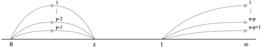
Figure 1: Contours of integration needed to represent $I_{p}(z)$.

Up to now we have not specified the contours of integration appearing in eq. (5.18). We shall use the canonical set of contours that give rise to the s-channel conformal blocks (see figure 1). We shall take the first $n-p+1$ integrals along a path lying on the real axis and joining the points $\tau=1$ and $\tau=\infty$. The remaining $p-1$ integrals will be taken along the segment $(0,z)$. Relabeling appropriately the integration variables, the $p^{th}$ conformal block can be written as:

$$I_{p}(z)\,=\,\int_{1}^{\infty}\,du_{1}\cdots\int_{1}^{u_{n-p}}\,du_{n-p+1}\int_{0}^{z}\,dv_{1}\cdots\int_{0}^{v_{p-2}}\,dv_{p-1}\,\lambda_{p}(z,\{u_{i}\},\{v_{i}\})\,\eta_{p}(\{u_{i}\},\{v_{i}\}).$$

(5.21)

In eq. (5.21), the quantities $\lambda_{p}(z,\{u_{i}\},\{v_{i}\})$ and $\eta_{p}(\{u_{i}\},\{v_{i}\})$ are, respectively, the functions $\lambda(z,\{\tau_{i}\})$ and $\eta(\{\tau_{i}\})$ after the relabelling of variables introduced above. By applying Wick’s theorem to the vacuum expectation value (5.19), one can readily prove that $\lambda_{p}(z,\{u_{i}\},\{v_{i}\})$ is given by:

$$\lambda_{p}(z,\{u_{i}\},\{v_{i}\})\,= \,z^{8j_{1}j_{2}\rho}\,(1-z)^{8j_{2}^{2}\rho}\,\prod_{i=1}^{n-p+1}\,u_{i}^{a}\,(u_{i}-z)^{b}\,(u_{i}-1)^{b}\,\prod_{i<j}(u_{i}-u_{j})^{2\rho}\times$$

$$\times\prod_{i=1}^{p-1}\,v_{i}^{a}\,(z-v_{i})^{b}\,(1-v_{i})^{b}\prod_{i<j}(v_{i}-v_{j})^{2\rho}\,\prod_{i=1}^{n-p+1}\,\prod_{j=1}^{p-1}(u_{i}-v_{j})^{2\rho},$$

where $\rho\,=\,\alpha_{0}^{2}/2$, $a\,=\,-2j_{1}\alpha_{0}^{2}$ and $b\,=\,-2j_{2}\alpha_{0}^{2}$. It is not difficult to obtain the non-analytical behaviour of the blocks around the point $z=0$. This behaviour is of the form:

$$I_{p}(z)\,\sim\,N_{p}\,z^{\gamma_{p}}\,,$$ (5.23)

where $N_{p}$ and $\gamma_{p}$ are constants. The latter can be written as a difference of conformal weights of the form:

$$\gamma_{p}\,=\,h_{j_{3}}\,-\,h_{j_{1}}\,-\,h_{j_{2}}\,.$$ (5.24)

The isospin $j_{3}$ has the interpretation of the isospin of the s-channel intermediate state. Its expression as a function of $p$ is:

$$j_{3}\,=\,j_{1}\,+\,j_{2}\,+{1\,-\,p\over 2}\,.$$ (5.25)

Notice that as $p=1,\cdots,4j_{2}+1$ the values taken by $j_{3}$ are $j_{1}-j_{2},j_{1}-j_{2}+{1\over 2},\cdots,j_{1}+j_{2}$, in agreement with the Clebsch-Gordan decomposition (2.13).

The physical correlation functions, which we shall denote by $G(z\,,\,\bar{z})$, can be obtained by combining holomorphic and antiholomorphic blocks in a monodromy invariant way:

$$G(z\,,\,\bar{z})\,=\,\sum_{p}\,X_{p}\,|\,I_{p}(z)\,|^{2}\,.$$ (5.26)

The coefficients $X_{p}$ have been computed in ref. [12]. The leading $z\rightarrow 0$ behaviour of $G(z\,,\,\bar{z})$ can be obtained by combining eqs. (5.23) and (5.26):

$$G(\,z\,,\,\bar{z}\,)\,\sim\,\sum_{p}\,\,\Bigl{[}\,{S_{p}\over|z|^{2\,(h_{j_{1}}+h_{j_{2}}-h_{j_{3}})}}\,+\,O(z)\,\Bigr{]}\,,$$ (5.27)

where the constants $S_{p}$ are given by:

$$S_{p}\,=\,X_{p}\,(N_{p})^{2}\,.$$ (5.28)

The quantities $S_{p}$ are related to the structure constants of the operator product algebra of the model. These constants, which we shall denote by $D_{j_{1},m_{1};j_{2},m_{2}}^{j_{3},m_{3}}$, appear in the leading terms of the OPE’s of the primary fields, namely:

$$\Phi_{m_{1}}^{j_{1}}(z_{1},\bar{z}_{1})\,\Phi_{m_{2}}^{j_{2}}(z_{2},\bar{z}_{2})\,=\,\sum_{j_{3},m_{3}}\,D_{j_{1},m_{1};j_{2},m_{2}}^{j_{3},m_{3}}\,\,\Bigl{[}\,{\Phi_{m_{3}}^{j_{3}}(z_{2},\bar{z}_{2})\over|z_{1}\,-z_{2}|^{2(h_{j_{1}}\,+\,h_{j_{2}}\,-\,h_{j_{3}})}}\,+\,O(z_{1}\,-z_{2})\,\Bigr{]}.$$ (5.29)

The two-point functions of the theory are normalized as:

$$<\,\Phi_{m_{1}}^{j_{1}}(z_{1},\bar{z}_{1})\,\Phi_{m_{2}}^{j_{2}}(z_{2},\bar{z}_{2})\,>\,=\,(-1)^{\sigma(j_{1},m_{1})}\,\,\,{\delta_{j_{1},j_{2}}\,\delta_{m_{1},-m_{2}}\over|z_{1}\,-z_{2}|^{4h_{j_{1}}}}\,,$$ (5.30)

where $\sigma(j,m)$ is $0$($1$) if the state $|j,m>$ has positive(negative) norm. Therefore, the structure constants must satisfy the constraint:

$$D_{j_{1},m_{1};j_{1},-m_{1}}^{0,0}\,=\,(-1)^{\sigma(j_{1},m_{1})}\,.$$ (5.31)

In order to relate the quantities $S_{p}$ of eq. (5.28) to the structure constants (5.31), let us use the OPE’s (5.29) in the correlator $G(\,z\,,\,\bar{z}\,)$. The result one gets is:

$$G(\,z\,,\,\bar{z}\,)\,\sim\,\sum_{j_{3},m_{3}}\,\,(-1)^{\sigma(j_{3},m_{3})}\,\,\Bigl{[}\,{[\,D_{j_{1},j_{1};j_{2},-j_{2}}^{j_{3},m_{3}}\,]^{2}\over|z|^{2\,(h_{j_{1}}+h_{j_{2}}-h_{j_{3}})}}+\,O(z)\,\Bigr{]}\,,$$ (5.32)

from which one we have the identification:

$$(-1)^{\sigma(j_{3},m_{3})}\,\,[\,D_{j_{1},j_{1};j_{2},-j_{2}}^{j_{3},m_{3}}\,]^{2}\,\,\sim\,\,S_{p}\,.$$ (5.33)

Using (5.33) it is possible to obtain the structure constants from our free field formalism [11]. Let us introduce the functions $\lambda(j)$ and ${\cal P}(j)$. The former is defined as:

$$\lambda(j)\,\equiv\,{\Gamma({j\over 2}\,+\,j\rho\,-\,[{j\over 2}])\over\Gamma({j\over 2}\,-\,j\rho\,-\,[{j\over 2}])}\,\,,$$ (5.34)

while ${\cal P}(j)$ is given by:

$${\cal P}(j)\,\equiv\,\prod_{i=1}^{j}\,\lambda(i)\,=\,\prod_{i=1}^{j}\,{\Gamma({i\over 2}\,+\,i\rho\,-\,[{i\over 2}])\over\Gamma({i\over 2}\,-\,i\rho\,-\,[{i\over 2}])}\,\,.$$ (5.35)

Let us also introduce the Clebsch-Gordan coefficients corresponding to the tensor product decomposition (2.13):

$$|\,j_{3},m_{3}\,>\,=\,\sum_{m_{1},m_{2}}\,C_{j_{1},m_{1};j_{2},m_{2}}^{j_{3},m_{3}}\,\,\,\,|j_{1},m_{1}>\otimes\,|j_{2},m_{2}>\,\,.$$ (5.36)

In terms of the quantities defined above, the structure constants can be written as [11]:

$$\Bigl{[}\,D_{j_{1},m_{1};j_{2},m_{2}}^{j_{3},m_{3}}\,\Bigr{]}^{2}\,= \,\Bigl{[}\,C_{j_{1},m_{1};j_{2},m_{2}}^{j_{3},m_{3}}\,\Bigr{]}^{4}\,\lambda(1)\,\,{\cal P}^{2}(2j_{1}+2j_{2}+2j_{3}+1)\,\times$$ (5.37)

$$\times\,\,\prod_{i=1}^{3}\,\,{\lambda(4j_{i}+1)\,{\cal P}^{2}(2j_{1}+2j_{2}+2j_{3}-4j_{i})\over{\cal P}^{2}(4j_{i}+1)}\,\,.$$

By studying the conditions under which the right-hand side of eq. (5.37) is non-vanishing we can obtain the fusion rules of the model. First of all, it is easy to verify that those fields with isospin $j\,\leq\,k/2$ close under multiplication. Actually, a detailed study of eq. (5.37) (see ref. [11]) leads to the fusion rule:

$$[j_{1}]\,\times\,[j_{2}]\,=\,\sum_{{j_{3}=|j_{1}-j_{2}|\atop}\atop 2(j_{3}-j_{1}-j_{2})\,\in\,{\rm Z}\kern-3.8pt{\rm Z}\kern 2.0pt}^{{\rm min}\,(\,j_{1}+j_{2}\,,\,k+{1\over 2}-j_{1}-j_{2}\,)}\,\,\,[j_{3}]\,\,,$$ (5.38)

which can be compared with the composition law of the finite algebra (eq. (2.13)).

6 Conclusions and final remarks

In previous sections we have reviewed a series of results which have been recently obtained for the CFT based on the osp${(1|2)}$ affine Lie superalgebra. The global picture emerging from these results is that the osp${(1|2)}$ current algebra is a perfectly solvable rational CFT. In order to complete this picture it would be desirable to study some other aspects of the theory. Let us mention some of them. First of all, one should explore the possibility of building a CFT for the admissible representations, with fractional levels and isospins given by eq. (4.9). The fusion rules for these representations have been determined in ref. [9] from the null vector decoupling conditions.

Coming back to the case in which the isospin is integer or half-integer and the level $k$ is a non-negative integer, it is interesting to study the crossing symmetry of the conformal blocks of the theory. One can employ [13] with this purpose the free field representation of section 5. The behaviour of the correlator of the theory under exchange symmetry, i.e. under the braiding and fusion operations, should be determined by a quantum deformation of the universal enveloping algebra of osp${(1|2)}$. Moreover, this behaviour could be used to define invariants for three-manifolds. The corresponding Chern-Simons theory, whose states are in one-to-one correspondence with the conformal blocks of the two-dimensional model, allows to define knot invariants. We have recently found [13] the relation of these invariants with the su(2) knot polynomials. Let us finally mention that, with these results at hand, one could also study the integrable deformation of the osp${(1|2)}$ CFT with the hope of finding new solvable massive field theories in two dimensions.

7 Acknowledgements

Two of us (JMSS and AVR) would like to thank the organizers of the workshop “Trends in Theoretical Physics” for their warm hospitality at La Plata. This work was supported in part by DGICYT under grant PB93-0344, by CICYT under grant AEN96-1673 and by the European Union TMR grant ERBFMRXCT960012.

References

• [1] For a review see J. Fuchs, “Affine Lie algebras and quantum groups”, Cambridge University Press, 1992 and S. Ketov, “Conformal Field Theory”, World Scientific, Singapore(1995).
• [2] M. Bershadsky and H. Ooguri, Phys. Lett. B229 (1989) 374.
• [3] A. M. Polyakov and A. B. Zamolodchikov, Mod. Phys. Lett. A3 (1988) 1213.
• [4] J. B. Fan and M. Yu, “G/G Gauged Supergroup Valued WZNW Field Theory”, Academia Sinica preprint AS-ITP-93-22, hep-th/9304123.
• [5] I. P. Ennes, J. M. Isidro and A. V. Ramallo, Int. J. Mod. Phys. A11 (1996)2379.
• [6] A. Pais and V. Rittenberg, J. Math. Phys. 16(1975) 2063; M. Scheunert, W. Nahn and V. Rittenberg, J. Math. Phys. 18(1977)155.
• [7] V. Kac and M. Wakimoto, Proc. Natl. Acad. Sci. USA 85 (1988)4956.
• [8] J. B. Fan and M. Yu, “Modules over affine Lie superalgebras” , Academia Sinica preprint AS-ITP-93-14, hep-th/9304122.
• [9] I. P. Ennes and A. V. Ramallo, Fusion rules and singular vectors of the osp${(1|2)}$ current algebra, Santiago preprint US-FT-12/97, hep-th/9704065, to appear in Nuclear Physics B.
• [10] B. Gordon, Quart. J. Math. Oxford Ser. (2) 12(1961)285.
• [11] I. P. Ennes, A. V. Ramallo and J. M. Sanchez de Santos, Phys. Lett. B389(1996)485; Nucl. Phys. B491 [PM] (1997) 574.
• [12] Vl.S.Dotsenko and V. A. Fateev Nucl. Phys. B240(1984)312; Nucl. Phys. B251(1985)691; Phys. Lett. B154 (1985)291.
• [13] I. P. Ennes, P. Ramadevi, A. V. Ramallo and J. M. Sanchez de Santos, “Duality in osp${(1|2)}$ Conformal Field Theory and link invariants”, preprint in preparation.