A Model of Graceful Exit in String Cosmology

Abstract

We construct, for the first time, a model of graceful exit transition from a dilaton-driven inflationary phase to a decelerated Friedman$-$Robertson$-$Walker era. Exploiting a demonstration that classical corrections can stabilize a high curvature string phase while the evolution is still in the weakly coupled regime, we show that if additional terms of the type that may result from quantum corrections to the string effective action exist, and induce violation of the null energy condition, then evolution towards a decelerated Friedman$-$Robertson$-$Walker phase is possible. We also observe that stabilizing the dilaton at a fixed value, either by capture in a potential minimum or by radiation production, may require that these quantum corrections are turned off, perhaps by non-perturbative effects or higher order contributions which overturn the null energy condition violation.

Preprint Number: BGU-PH-97/11

I INTRODUCTION

An inflationary scenario [1, 2], inspired by duality symmetries of string cosmology equations [1, 3, 4], is based on the fact that cosmological solutions to string dilaton-gravity come in duality-related pairs, the plus branch $(+)$, and the minus branch $(-)$ [5]. The $(+)$ branch has kinetic inflationary solutions in which the Hubble parameter increases with time. The minus branch $(-)$ can be connected smoothly to a standard Friedman$-$Robertson$-$Walker (FRW) decelerated expansion of the Universe with constant dilaton. The scenario (the so called “pre-big-bang” scenario) is that evolution of the Universe starts from a state of very small curvature and coupling and then undergoes a long phase of dilaton-driven kinetic inflation described by the $(+)$ branch and at some later time joins smoothly standard radiation dominated cosmological evolution, thus giving rise to a singularity free inflationary cosmology. Recently, the required initial conditions of the Universe in this scenario were discussed [6]. Our focus in this paper is mainly on the final fate of the Universe at late times and we simply assume that the correct initial conditions were chosen such that a long dilaton-driven inflationary phase was indeed part of the evolution.

The graceful exit transition from the initial long phase of dilaton-driven kinetic inflation to the subsequent standard radiation dominated evolution has been a subject of many investigations [7, 8, 9, 10]. In [5] it was argued, and later proved [11], that such a transition cannot occur while curvature was below the string scale and the string coupling was still weak, leading to the conclusion that an intermediate “string phase” of high curvature (previously suggested as a possibility [1, 2]) or strong coupling is actually required [12].

In [7] we proposed to use an effective description in terms of sources that represent arbitrary corrections to the lowest order equations. We were able to relate necessary conditions for graceful exit to energy conditions appearing in singularity theorems of Einstein’s general relativity [13]. In particular, we showed that a successful exit requires violations of the null energy condition (NEC). Since most classical sources obey NEC this conclusion hints that quantum effects, known to violate NEC in some cases, may be the correct sources to look at. To briefly recap the relevant results of [7] we need to recall that there are different conformal frames in which to describe the equations. These are related by local field redefinitions which, supposedly, do not affect physical observables [14]. The two frames that we use are the string frame ($\underline{S\ }\!\!|$ ) and the “lowest order Einstein frame” ($\underline{E\ }\!\!|$ ) in which the lowest order classical action kinetic terms of gravity and the dilaton are diagonal. For brevity we call $\underline{E\ }\!\!|$ the Einstein frame. The general analysis of [7] resulted in a set of necessary conditions on the evolution in terms of the Hubble parameters $H_{S}$ in the string frame and $H_{E}$ in the Einstein frame and the dilaton $\phi$. We include them for completeness

• Initial conditions of a (+) branch and $H_{S},\dot{\phi}>0$ require $H_{E}<0$.

• A branch change from (+) to $(-)$ has to occur while $H_{E}<0$.

• A successful escape and exit completion requires NEC violation accompanied by a bounce in $\underline{E\ }\!\!|$ after the branch change has occurred, ending up with $H_{E}>0$.

• Further evolution is required to bring about a radiation dominated era in which the dilaton effectively decouples from the “matter” sources.

The question we set to answer in this paper is the following. Suppose that effective sources of the type that are expected to appear as corrections to the lowest order effective action of strings do provide NEC violation. Then would a complete exit transition actually occur? We answer this question in the affirmative, but some surprising obstacles are found on the way and we also suggest ways to overcome these obstacles.

Because in our scenario the Universe evolves towards higher curvatures and stronger coupling, there will be some time when the lowest order effective action can no longer reliably describe the dynamics and it must be corrected. Corrections to the lowest order effective action come from two sources. The first are classical corrections, due to the finite size of strings, arising when the fields are varying over the string length scale $\lambda_{s}=\sqrt{\alpha^{\prime}}$. These terms are important in the regime of large curvature. The second are quantum loop corrections. The loop expansion is parameterized by powers of the string coupling parameter $e^{\phi}=g_{string}^{2}$, which in the models that we consider is, of course, time dependent. So quantum corrections will become important when the dilaton becomes large, the regime we refer to as strong coupling.

In this paper we make use of both types of corrections. The role of $\alpha^{\prime}$ corrections [10] is to create an attractive fixed point which stabilizes the evolution in a high curvature regime with linearly growing dilaton. The basin of attraction of this fixed point is large enough to allow it to be reached from generic initial conditions. Further, the location of this fixed point is such it forces the evolution to undergo a branch change, and all of this may occur for small values of the dilaton (weak coupling) so the quantum corrections can be ignored. With the linearly growing dilaton, the quantum corrections will eventually become important. It is these we will attempt to use to let the Universe escape the fixed point and complete the transition to a decelerated FRW evolution. We allow ourselves the freedom to choose the coefficients of the quantum correction terms arbitrarily, in particular, their sign is chosen so as to induce NEC violation. Our reasoning for allowing this freedom stems in part from a lack of any real string calculations and in part by our desire to verify by constructing explicit examples the general arguments of [7].

We use the general framework set up in, and rely for analytical calculations mostly on [7]. We perform numerical integration of specific equations with limited new analytical considerations. We show, by constructing explicit examples, that a complete exit transition is not forbidden, which, of course, does not yet prove that in string theory it actually occurs. For that, an explicit string computation of quantum correction terms is necessary. This may also require taking into account the backreaction of the particles produced during the dilaton-driven phase.

A by-product of our analysis is a detailed description of the high-curvature (“string”) phase in between the dilaton-driven inflationary phase and the decelerated FRW phase. We obtain a more complicated phase than the one postulated in [12] with non-constant $\dot{\phi}$ and $H_{S}$. We do not take the details of the evolution in the string phase too seriously, because the terms that determine those details have arbitrary coefficients. However, our examples could be taken as an indication of what the real string phase may eventually look like.

The paper is organized as follows. In section II we present and discuss solutions which exhibit branch change and exit completion with $\alpha^{\prime}$ and quantum corrections. In section III we explain the remaining problem of correction dominated evolution, show how to model a shut-off of the corrections and verify that once corrections are shut off, the usual decelerated evolution such as radiation domination or capturing of the dilaton in a minimum of a potential may follow. We summarize our results and explain which further calculations are necessary to reach a conclusive statement about exit transition in string models. In a technical appendix we outline details of derivation of equations of motion, numerical integration etc.

II A Model for Exit Completion

String theory effective action in four dimensions takes the following general form,

$$S_{eff}^{{\hbox{$\underline{S\ }\!\!|$\ }}}=\int d^{4}x\left\{\sqrt{-g}\left[\frac{e^{-\phi}}{16\pi\alpha^{\prime}}\left(R+\partial_{\mu}\phi\partial^{\mu}\phi\right)\right]+\hbox{$\frac{1}{2}$}\sqrt{-g}{\cal L}_{c}\right\},$$ (1)

where $g_{\mu\nu}$ is the 4-d metric and $\phi$ is the dilaton, the effective action is written here in the string frame ($\underline{S\ }\!\!|$ ). The Lagrangian ${\cal L}_{c}$ may contain arbitrary corrections to the lowest order 4-d action coming from a variety of sources as specified below.

We are interested in solutions to the equations of motion derived from the action (1) of the FRW type with vanishing spatial curvature (non-vanishing spatial curvature may be included as an effective source in the equations) $ds^{2}=-dt_{S}^{2}+a_{S}^{2}(t)dx_{i}dx^{i}$ and $\phi=\phi(t)$. We will assemble the equations of motion by deriving the correction energy-momentum tensor $T_{\mu\nu}=\frac{1}{\sqrt{-g}}\frac{\delta\sqrt{-g}{\cal L}_{c}}{\delta g^{\mu\nu}}$, which will have the form $T^{\mu}_{\ \nu}=diag(\rho,-p,-p,-p)$. In addition we have another form of source term arising from the variation by $\phi$ equation, $\Delta_{\phi}{\cal L}_{c}=\hbox{$\frac{1}{2}$}\frac{1}{\sqrt{-g}}\frac{\delta\sqrt{-g}{\cal L}_{c}}{\delta\phi}$.

In terms of these sources the equations of motion are

$$3H_{S}^{2}+\hbox{$\frac{1}{2}$}\dot{\phi}^{2}-3H_{S}\dot{\phi} = \hbox{$\frac{1}{2}$}e^{\phi}\rho$$ (2)

$$-2\dot{H}_{S}-3H_{S}^{2}+2H_{S}\dot{\phi}-\hbox{$\frac{1}{2}$}\dot{\phi}^{2}+\ddot{\phi} = \hbox{$\frac{1}{2}$}e^{\phi}p$$ (3)

$$3\dot{H}_{S}+6H_{S}^{2}-3H_{S}\dot{\phi}+\hbox{$\frac{1}{2}$}\dot{\phi}^{2}-\ddot{\phi} = \hbox{$\frac{1}{2}$}e^{\phi}\Delta_{\phi}{\cal L}_{c}$$ (4)

$$\dot{\rho}+3H_{S}(\rho+p) = -\Delta_{\phi}{\cal L}_{c}\dot{\phi},$$ (5)

$H_{S}=\dot{a}_{S}/a_{S}$, and we have fixed our units such that $16\pi\alpha^{\prime}=1$.

We will make the split

$${\cal L}_{c}={\cal L}_{\alpha^{\prime}}+{\cal L}_{q}+{\cal L}_{m}\\$$ (6)

and we will divide up the source terms analogously. For example, $\rho=\rho_{\alpha^{\prime}}+\rho_{q}+\rho_{m}$. We take, for concreteness, the Lagrangian ${\cal L}_{\alpha^{\prime}}$ to be of the specific form of the $\alpha^{\prime}$ classical corrections proposed in [10],

$$\hbox{$\frac{1}{2}$}{\cal L}_{\alpha^{\prime}}=e^{-\phi}(\frac{R_{GB}^{2}}{4}-\frac{(\nabla\phi)^{4}}{4}).$$ (7)

The contribution of this term to the effective sources is

$$\rho_{\alpha^{\prime}} = e^{-\phi}(6H_{S}^{3}\dot{\phi}-\frac{3\dot{\phi}^{4}}{4})$$ (8)

$$p_{\alpha^{\prime}} = e^{-\phi}(-4H_{S}^{3}\dot{\phi}-4H_{S}\dot{H}_{S}\dot{\phi}+2H_{S}^{2}\dot{\phi}^{2}-\frac{\dot{\phi}^{4}}{4}-2H_{S}^{2}\ddot{\phi})$$ (9)

$$\Delta_{\phi}{\cal L}_{\alpha^{\prime}} = e^{-\phi}(-6H_{S}^{4}-6H_{S}^{2}\dot{H}_{S}+3H_{S}\dot{\phi}^{3}-\frac{3\dot{\phi}^{4}}{4}+3\dot{\phi}^{2}\ddot{\phi}).$$ (10)

Although we have fixed our units differently from [10] (where $k\alpha^{\prime}=1$, k depending on the species of string theory), we have chosen the coefficient of this term so as to lead to solutions which are numerically identical to theirs for purposes of comparison.

The Lagrangian ${\cal L}_{q}$ will designate quantum loop corrections parameterized by powers of $e^{\phi}$. We will examine a variety of candidates for ${\cal L}_{q}$. The Lagrangian ${\cal L}_{m}$ will represent such things as radiation or a dilaton potential when we discuss the final transition to radiation domination and a fixed dilaton.

Setting ${\cal L}_{q}={\cal L}_{m}=0$, for the moment, we integrate the equations of motion starting from initial conditions near the $(+)$ branch vacuum. To do this we solve (3) and (4) for the highest derivatives of $H_{S}$ and $\phi$ and use (2) as a constraint on the initial conditions. The conservation equation (5) is an identity owing to the usual redundancy in the equations, only when we add radiation to the system will we use this equation in the evolution. We recover the results of [10] in four dimensions where they find attraction into a fixed point at $H_{S}=0.616...,\dot{\phi}=1.404...$.

As shown in Fig. 1a the solution begins near the $(+)$ branch vacuum and makes a branch change but does not “complete” the exit by proceeding to the $\rho>0$ region. The quantity characterizing branch sign is plotted in Fig. 1e. We examined more general forms of this Lagrangian involving different coefficients. Varying the coefficients moves the fixed point. For some ratios of coefficients the solutions encounter singularities before reaching the fixed point (we discuss the form of these singularities in section 3) but other ratios yield solutions of the same generic type as we have presented here.

In spite of considerable progress we still need to look more closely at the sources and Einstein frame evolution to answer the question of how close we have come to the true goal of decelerated FRW evolution.

The evolution of $\rho$ and $p$ is easily found by substituting the solution back into the equations of motion and solving for the sources. We see that this phase does violate NEC in the string frame. However, recalling our stronger claim that there should also be NEC violation in the “lowest order Einstein frame” (denoted with a subscript $E$ and as explained in the introduction, many times for brevity called just the Einstein frame), we can compute the value of the Einstein frame sources by finding the Hubble parameter $H_{E}$ and its derivative $\dot{H}_{E}$,

$$H_{E} = e^{\phi/2}(H_{S}-\hbox{$\frac{1}{2}$}\dot{\phi})$$ (11)

$$\dot{H}_{E} = e^{\phi}(\dot{H}_{S}-\hbox{$\frac{1}{2}$}\ddot{\phi}+\hbox{$\frac{1}{2}$}\dot{\phi}H_{S}-\frac{\dot{\phi}^{2}}{4})$$ (12)

All quantities on the right hand side of these are given strictly in terms of string frame quantities and time. The Einstein equations are,

$$3H_{E}^{2} = \hbox{$\frac{1}{2}$}\rho_{E}$$ (13)

$$3H_{E}^{2}+2\dot{H}_{E} = -\hbox{$\frac{1}{2}$}p_{E}$$ (14)

Notice that we have absorbed the dilaton kinetic energy into the definition of $\rho_{E}$ and $p_{E}$.

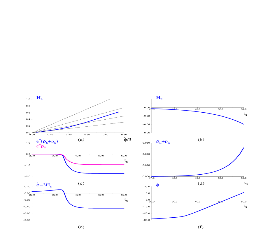
FIG. 1.: A solution to the classical equations with only $\alpha^{\prime}$ corrections, ${\cal L}_{q}={\cal L}_{m}=0$. (a) Evolution in the $(\dot{\phi}/3,H_{S})$ plane. The four lines plotted are, in order of increasing slope, the $(+)$ branch vacuum ($\rho=0,\dot{\phi}=(3+3^{1/2})H_{S}$), branch change ($\dot{\phi}=3H_{S}$), Einstein frame “bounce” ($\dot{\phi}=2H_{S}$) and $(-)$ branch vacuum ($\rho=0,\dot{\phi}=(3-3^{1/2})H_{S}$). The cross is at the location of the fixed point. The remaining figures are various quantities plotted as a function of string time. (b) The Einstein frame Hubble parameter $H_{E}$. (c) The string frame source terms $e^{\phi}(\rho_{S}+p_{S})$ and $e^{\phi}\rho_{S}$. (d) The Einstein frame source term $\rho_{E}+p_{E}$. (e) $\dot{\phi}-3H_{S}$, a quantity indicating branch sign. (In section III this figure will be replaced by $e^{\phi}\rho_{S}$ from (c)), (f) $\phi$ evolution. Initial conditions at $t=0$, $\phi=-30,H_{S}=0.0148529,\dot{\phi}=0.0699602$. The following figures share these initial conditions, since quantum corrections are very small at this time. The $\phi$ evolution may be started at arbitrarily small values by evolving these initial conditions further backward towards the $(+)$ branch vacuum.

The resulting sources and $H_{E}$ are plotted in Fig. 1b,c,d. From the figures we see that there is no violation of NEC in the Einstein frame, corresponding to the fact that there is no “bounce”. This solution represents a singular collapse in the Einstein frame because of the linearly increasing dilaton plotted in Fig. 1f. In terms of sources this suggests that there is insufficient NEC violation and that the addition of conventional sources to ${\cal L}_{m}$, like radiation, which do not violate NEC cannot help the completion of the exit transition.

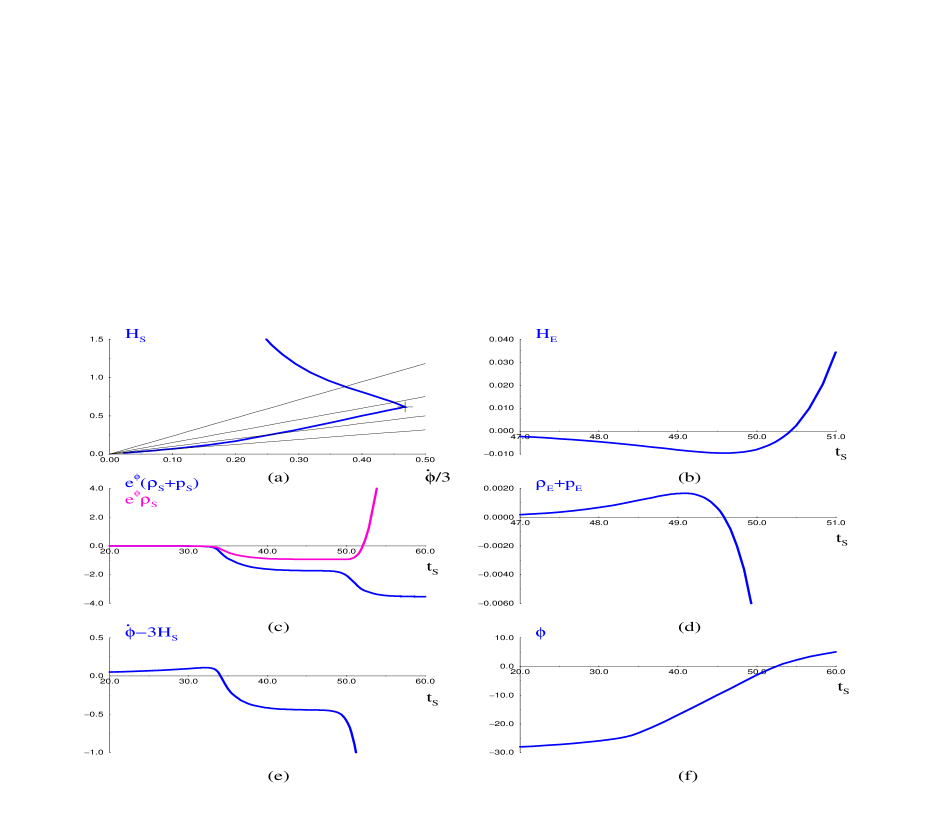
FIG. 2.: $\hbox{$\frac{1}{2}$}{\cal L}_{q}^{\phi}=-(\nabla\phi)^{4}$, ${\cal L}_{m}=0$. See Fig. 1 caption for details and initial conditions.

Perhaps generically any correction violating NEC strongly enough will complete the transition. In particular, we consider terms modeling the form of quantum loop corrections parameterized by powers of $e^{\phi}$. For example, at one loop,

$$\hbox{$\frac{1}{2}$}{\cal L}_{q}^{\phi} = -(\nabla\phi)^{4}$$ (15)

$$\rho_{q}^{\phi} = -3\dot{\phi}^{4}$$ (16)

$$p_{q}^{\phi} = -\dot{\phi}^{4}$$ (17)

$$\Delta_{\phi}{\cal L}_{q}^{\phi} = 12(H_{S}\dot{\phi}^{3}+\dot{\phi}^{2}\ddot{\phi})$$ (18)

As long as we include only one order of loop correction, the overall coefficient of our corrections can be absorbed by a shift of $\phi$, and it therefore determines the value of $\phi$ at which the quantum corrections begin to be important, but doesn’t lead to qualitatively different behavior. So at this stage we choose coefficients of order unity and after these preliminary investigations are complete, we will choose more realistic values.

Clearly, because of the factor of $e^{\phi}$ on the right hand side of equations (2), (3) this ${\cal L}_{q}^{\phi}$ can give us NEC violation of increasing strength as $\phi$ increases. We show the results of the numerical integration by presenting the same suite of figures as in the previous case in Fig. 2. In this case we have chosen to graph the sources for a range of time emphasizing the Einstein frame bounce. As hoped, the solution now proceeds into the $\rho>0$ region triggered by increased NEC violation in the string frame. We also see the accompanying Einstein frame NEC violation and bounce. Notice that the bounce occurs quickly, during a few units of time, compared with the very long duration of the dilaton-driven phase near the $(+)$ vacuum.

However, inspecting the solution at late times shows the dominant terms in the equations of motion are:

$$-6H_{S}^{2}-3e^{\phi}\dot{\phi}^{4}+6H_{S}^{3}\dot{\phi} = 0$$ (19)

$$-6H_{S}^{2}+e^{\phi}\dot{\phi}^{4}+4H_{S}^{3}\dot{\phi} = 0$$ (20)

$$-6H_{S}^{4}+12e^{\phi}H_{S}\dot{\phi}^{3} = 0$$ (21)

This system has the solution,

$$H_{S} = {2t\over 3}$$ (22)

$$\phi = \log({t^{6}\over 39366})$$ (23)

approximating the nature of the true solution at late times.

This form confirms that the solution has unbounded growth in the curvature and dilaton. Nonetheless, we have succeeded in our aim of completing the exit to the $\rho>0$ region of phase space. It may appear that we are now facing a new “graceful exit” problem since the equations of motion at late times are dominated by corrections, spoiling the expected stability of a $(-)$ branch. We suggest that the source of this instability is the continued NEC violation and will search for a cure in the next section.

To further explore the sufficiency of NEC violation for exit we examine another generic form of one loop quantum correction,

$${\cal L}_{q}^{R^{2}} = R^{2}$$ (24)

$$\rho_{q}^{R^{2}} = -108H_{S}^{2}\dot{H}_{S}+18\dot{H}_{S}^{2}-36H_{S}\ddot{H}_{S}$$ (25)

$$p_{q}^{R^{2}} = 108H_{S}^{2}\dot{H}_{S}+54\dot{H}_{S}^{2}+72H_{S}\ddot{H}_{S}+12H_{S}^{(3)}$$ (26)

$$\Delta_{\phi}{\cal L}_{q}^{R^{2}} = 0$$ (27)

We immediately notice that for evolution strictly in the fixed point, where $H_{S}=constant$, this correction will be zero indicating it will not effectively contribute to NEC violation. Furthermore, this introduces higher derivatives into the equations of motion, which in turn introduces dangerous pathologies into the solutions [15].

These pathologies come from the extra degrees of freedom in the system coming from the extra initial conditions that need to be imposed. These extra degrees of freedom are associated with unstable modes of the solutions which we regard as physically spurious, since they are solutions in which the “correction” becomes much larger than the terms to which it is supposed to be a small correction. Reference [15] suggests two remedies to this problem. The first is “reduction of order”, in which we differentiate the large terms in the equations of motion (in this case the tree level terms) and use them to rewrite the higher derivatives in terms of lower derivatives, justified by the assumption the corrections will remain small. The second is simply to carefully chose initial conditions to avoid the unstable modes.

Since our purpose is to make a qualitative survey of the effect of corrections and the reduction of order prescription is computationally prohibitive, we take the second approach and choose initial conditions so that the evolution is not dominated by the corrections for a reasonable span of time. Exploring these solutions confirms that ${\cal L}_{q}^{R^{2}}$ corrections themselves do not help the exit process. The other one loop curvature squared terms, $R^{\mu\nu}R_{\mu\nu}$ and $R^{\mu\nu\sigma\rho}R_{\mu\nu\sigma\rho}$ yield sources which are constant multiples of those of $R^{2}$, and as is well known, the Gauss-Bonnet combination, which does not contribute higher derivatives, vanishes in the equations of motion.

But putting curvature squared terms together with corrections that do not vanish in the fixed point, for example ${\cal L}_{q}={\cal L}_{q}^{\phi}-\frac{{\cal L}_{q}^{R^{2}}}{3}$, does yield qualitatively different solutions which do exit, in this case a solution approaching string frame deSitter (with constant $H_{S}$), though again with still growing dilaton as illustrated in Fig. 3. We set our initial conditions near a later phase of the $(+)$ branch vacuum to avoid instabilities.

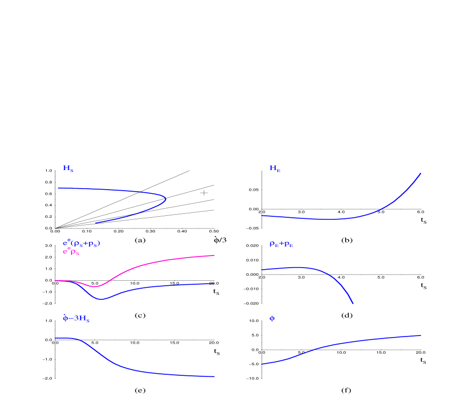
FIG. 3.: ${\cal L}_{q}={\cal L}_{q}^{\phi}-\frac{1}{3}{\cal L}_{q}^{R^{2}}$, ${\cal L}_{m}=0$. Initial conditions at $t=0$, $\phi=-5$, $H_{S}=0.0926031$, $\dot{\phi}=0.383925$, $\dot{H}_{S}=0.018527$, $\ddot{H}_{S}=0.0260335$. See Fig. 1 caption for explanation.

Finally, we present a two loop Gauss-Bonnet correction which we choose because it represents the influence of curvature squared terms but does not contribute higher derivative terms.

$$\hbox{$\frac{1}{2}$}{\cal L}_{q}^{R^{2}_{GB}} = e^{\phi}R^{2}_{GB}$$ (28)

$$\rho_{q}^{R^{2}_{GB}} = e^{\phi}(-24H_{S}^{3}\dot{\phi})$$ (29)

$$p_{q}^{R^{2}_{GB}} = e^{\phi}(16H_{S}^{3}\dot{\phi}+16H_{S}\dot{H}_{S}\dot{\phi}+8H_{S}^{2}\dot{\phi}^{2}+8H_{S}^{2}\ddot{\phi})$$ (30)

$$\Delta_{\phi}{\cal L}_{q}^{R^{2}_{GB}} = e^{\phi}(24H_{S}^{4}+24H_{S}^{2}\dot{H}_{S})$$ (31)

Again we find that introducing this correction with an appropriate sign can complete the transition to $\rho>0$ as in Fig. 4, but with increasing domination by the correction terms leading to a singularity soon after the transition. We have also tried other combinations of sources with different coefficients and found that many of them yield solutions that are similar to the ones we presented, leading us to believe that our result are quite general and do not depend in a strong way on particular initial conditions or coefficients.

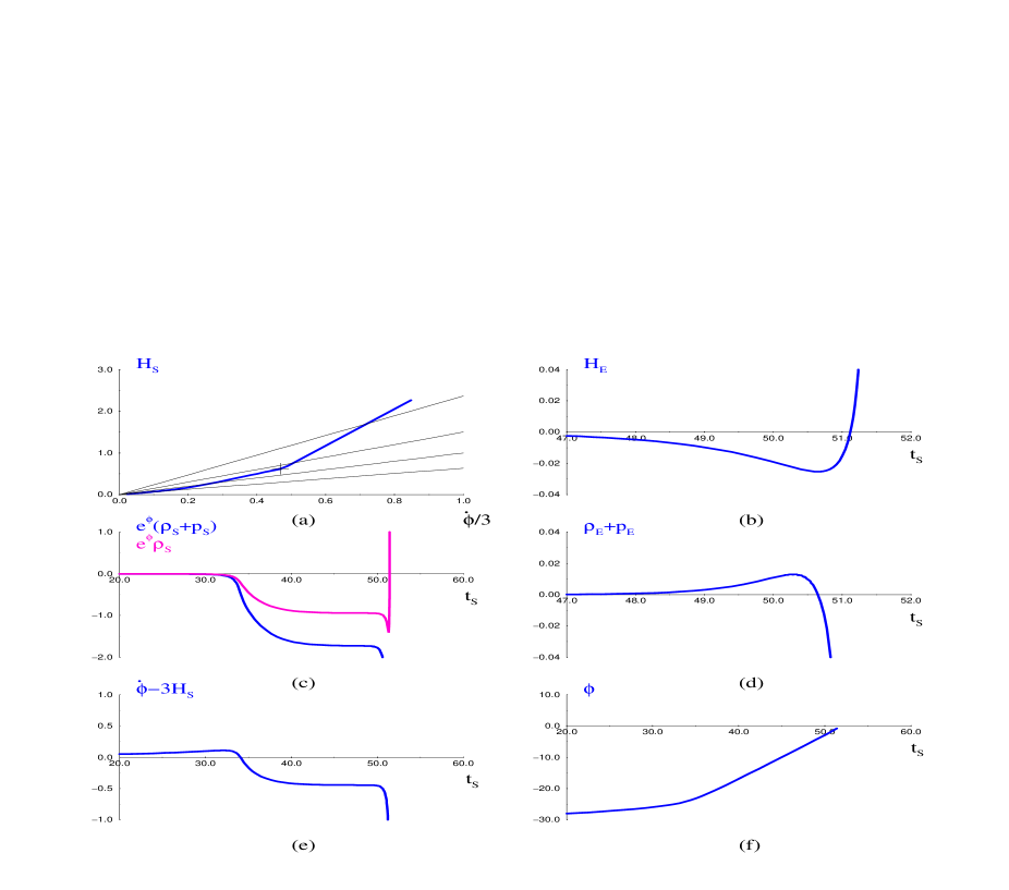
FIG. 4.: $\hbox{$\frac{1}{2}$}{\cal L}_{q}^{R^{2}_{GB}}=e^{\phi}R^{2}_{GB}$, ${\cal L}_{m}=0$. See Fig. 1 caption for details and initial conditions.

In summary, we have seen that generic forms of quantum corrections can complete the exit from the fixed point of [10] to the region of $\rho>0$, showing the NEC violation is not only necessary, but is in some sense sufficient. The resulting solutions are quite varied, but we have also noted they have unbounded growth of the dilaton at late times, continue to be dominated by corrections and continue to violate NEC. In spite of being $(-)$ branch solutions they are still unstable. However, inducing the exit seems to be a generic property of NEC violation and not of the specific form of the corrections. In the next section we will attack this new exit problem, the exit from the epoch of correction domination.

III A Model for Transition to Decelerated and Stable Evolution

We have seen that by using plausible forms for quantum corrections we can induce NEC violation and push the evolutions into a region we would like to call a completed exit. However, we have also seen that these evolutions are dominated by the corrections and have singular behavior unlike the desired $(-)$ branch solutions. We associate this behavior with two overlapping sources. First is the continued NEC violation itself, which tends to feed accelerated evolution in the Einstein frame. Second, and more directly, it is the continuing growth of $\phi$ that supports the strength of the quantum correction terms through the powers of $e^{\phi}$ occurring in the equations of motion.

Since these solutions do not spontaneously suppress the corrections we might hope that simply controlling the growth of the dilaton would tame the solutions. This can be done by modeling radiation production, which can slow the change in the dilaton through the $3H_{S}\dot{\phi}$ “friction” term in (4), or more directly by capturing the dilaton in a potential minimum.

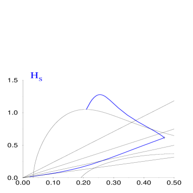
FIG. 5.: ${\cal L}_{q}={\cal L}_{q}^{\phi}$, ${\cal L}_{m}=-0.02\phi^{2}e^{\phi}$. Quantities plotted and initial conditions are as in Fig. 1a. Also shown are the singularity curves, defined in the text. The right curve is for $\phi\rightarrow-\infty$ and the left curve is for the value of $\phi$ at which the solution hits the curve.

Concentrating on the simplest of the NEC violating quantum corrections, (15), we are surprised to find obstacles to this program. Attempting to moderate the evolution through the use of a potential strong enough to affect the solution actually drives the solution into cusp singularities (singularities in $\ddot{\phi}$ and $\dot{H}_{S}$). The sources for a potential are:

$$\hbox{$\frac{1}{2}$}{\cal L}_{m}^{V} = V(\phi)$$ (32)

$$\rho_{m}^{V} = -V(\phi)$$ (33)

$$p_{m}^{V} = V(\phi)$$ (34)

$$\Delta_{\phi}{\cal L}_{m}^{V} = V^{\prime}(\phi)$$ (35)

We illustrate a particular case in Fig. 5, with $V(\phi)=-0.01\phi^{2}e^{\phi}$. We have added graphs of the locations of the singularity curves. The curve on the right is the location of the singularities at $\phi\rightarrow-\infty$. The curve on the left is their location when the solution collides with them. Adding radiation can produce similar singularities or it is quickly redshifted away by the growing $H_{S}$.

The source of these singularities is easy to understand mathematically. The sources introduce additional terms containing the highest derivatives $\dot{H}_{S}$ and $\ddot{\phi}$ to the terms coming from the lowest order terms in the action. When we solve the equations of motion for $\dot{H}_{S}$ and $\ddot{\phi}$ in terms of the lower derivatives we find a denominator which has, in general, zeros in the $(x,y)$ plane, where $x=\dot{\phi}/3$ and $y=H_{S}$. In this particular case this leads to the equation for the singularity curves:

$${1\over 3}-9\,{x^{2}}-36\,{e^{\phi(t)}}\,{x^{2}}+2\,x\,y+27\,{x^{3}}\,y+108\,{e^{\phi(t)}}\,{x^{3}}\,y+2\,{y^{2}}+\,{y^{4}}=0$$ (36)

The terms containing the $e^{\phi}$ are coming from the quantum correction, so that the location of the singularity curves is now a function of $\phi$.

Perversely, the singularity curves follow the solution towards small $\dot{\phi}$ and large $H_{S}$. So any attempt to tinker with the solution causes it to collide with them. Modeling the production of radiation produces a similar effect. While we do not have a direct physical interpretation of these singularities we do regard them as an indication of the general instability of NEC violating solutions.

FIG. 6.: ${\cal L}_{q}={\cal L}_{q}^{f(\phi)}$, $f(\phi)=\hbox{$\frac{1}{2}$}e^{6}(1-\tanh(8\phi+36))$. See Fig. 1 caption for details and initial conditions. All quantities are nonsingular, but peaks are out of scale to emphasize details.

A direct approach to completing the exit transition is to assume that there exists some mechanism that shuts off the correction terms, and hence, NEC violation. A concrete way of modeling such an idea is simply replacing the quantum correction in the action with $f(\phi){\cal L}_{q}^{\phi}$ where $f(\phi)$ is a positive constant for $\phi<\phi_{0}$ for some constant $\phi_{0}$ and then smoothly goes to zero, so $f(\phi)$ has the form of a smoothed step function. This successfully eliminates the loop corrections at late times so the dilaton may be easily captured by a potential or slowed by radiation production as shown in Fig. 6. In this suite of figures we have dropped the branch sign graph, since all of the following solutions are similar in that region of the evolution and have now chosen a range of time to graph the sources emphasizing the epoch when NEC violation ceases and the evolution becomes decelerated. We have also tinkered with the normalization of this term so the figure may be directly compared with the previous figures. While we have exactly the desired behavior, a function like $f(\phi)$ will not appear by summing a few terms in the loop expansion.

$$\hbox{$\frac{1}{2}$}{\cal L}_{q}^{f(\phi)} = -f(\phi)(\nabla\phi)^{4}$$ (37)

$$\rho_{q}^{f(\phi)} = -3f(\phi)\dot{\phi}^{4}$$ (38)

$$p_{q}^{f(\phi)} = -f(\phi)\dot{\phi}^{4}$$ (39)

$$\Delta_{\phi}{\cal L}_{q}^{f(\phi)} = 12f(\phi)H_{S}\dot{\phi}^{3}+3f^{\prime}(\phi)\dot{\phi}^{4}+12f(\phi)\dot{\phi}^{2}\ddot{\phi}$$ (40)

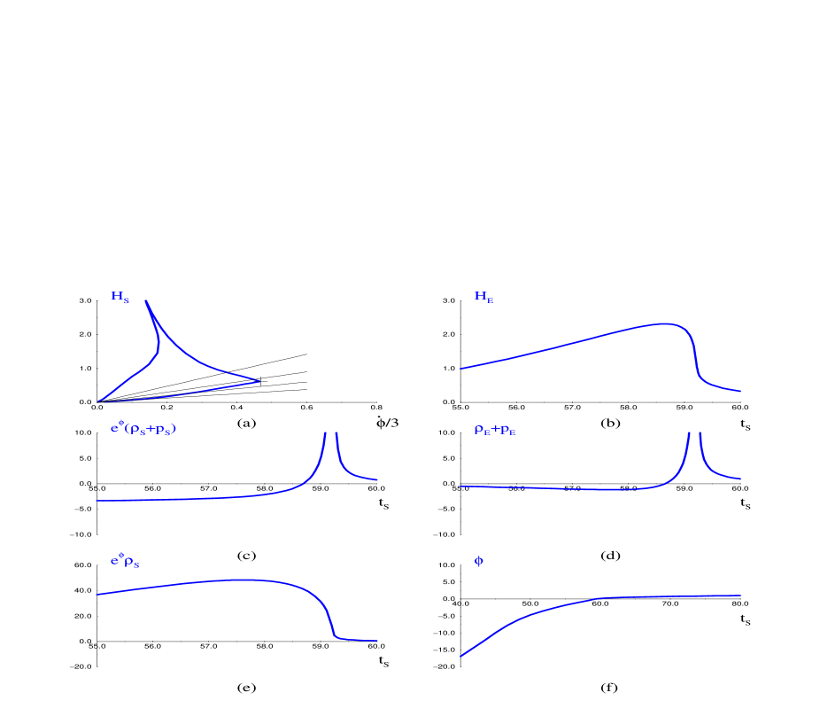
FIG. 7.: ${\cal L}_{q}=1000{\cal L}_{q}^{\phi}+1000{\cal L}_{q}^{2\phi}$. The peaks of $e^{\phi}(\rho_{S}+p_{S})\simeq 55$ and $\rho_{E}+p_{E}\simeq 55$ have been cut off to emphasize the sign change, but all quantities are non-singular. See Fig. 1 caption for details and initial conditions.

However, we have found that a complete suppression of the quantum corrections is not necessary. Suspecting that the instabilities are due to continued NEC violation we propose what is, perhaps, a simpler model. Since the NEC violation was induced in our models by one loop quantum corrections, higher loop terms can suppress the NEC violation once it is no longer needed if they have the correct sign. For example, a two loop contribution of the form,

$$\hbox{$\frac{1}{2}$}{\cal L}_{q}^{2\phi} = e^{\phi}(\nabla\phi)^{4}$$ (41)

$$\rho_{q}^{2\phi} = 3e^{\phi}\dot{\phi}^{4}$$ (42)

$$p_{q}^{2\phi} = e^{\phi}\dot{\phi}^{4}$$ (43)

$$\Delta_{\phi}{\cal L}_{q}^{2\phi} = -e^{\phi}(12H_{S}\dot{\phi}^{3}+3\dot{\phi}^{4}+12\dot{\phi}^{2}\ddot{\phi})$$ (44)

can overwhelm the one loop NEC violation when $\phi$ becomes large enough. Since now the scaling of different terms with respect to a shift in the dilaton (which determines the value of the string coupling at which various terms become important) is more complicated we will introduce these corrections with explicit large coefficients accounting for the expected large number of degrees of freedom contributing to the loop corrections. We expect, in string theory, large and approximately the same order of magnitude coefficients for certain one and two loop corrections, which, perhaps, may even be justified with some large N techniques. Taking ${\cal L}_{q}=C_{1}{\cal L}_{q}^{\phi}+C_{2}{\cal L}_{q}^{2\phi}$ we observe that since the sources occur in the equations of motion with coefficients $C_{1}e^{\phi}$ and $C_{2}e^{2\phi}$ respectively, and these terms will be important to the evolution when these coefficients are of order unity, then having $C_{1}\approx C_{2}\gg 1$ leads to a situation where the one-loop terms become important at a smaller value of $\phi$ (and therefore an earlier time) than the two-loop. Thus we can still have an era of NEC violation which is ended by the onset of the two-loop terms in a rather natural way. We have numerically solved the equations for a range of coefficients and observe a generic behaviour which we illustrate with the specific example in Fig. 7.

We show the results of a sample evolution in Fig. 7. For the graphs of $H_{E}$ and $\rho_{E}+p_{E}$ we choose a time range to emphasize the epoch after the bounce, where NEC violation ceases and the evolution becomes decelerated FRW. In Fig. 8 we show that with this form of corrections the behavior is mild enough that it is easy to capture the dilaton into a potential minimum. In these figures we emphasize the late phase where the dilaton is rolling around the potential minimum, but the early evolution is indistinguishable from Fig. 7.

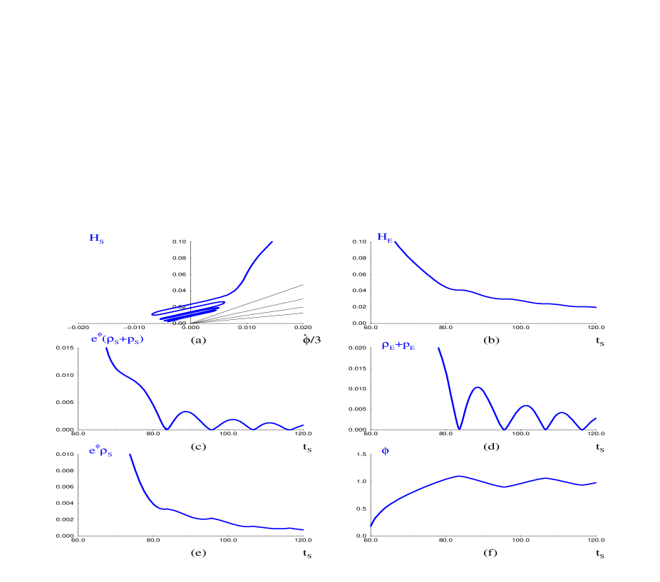
FIG. 8.: $\hbox{$\frac{1}{2}$}{\cal L}_{q}=1000{\cal L}_{q}^{\phi}+1000{\cal L}_{q}^{2\phi},\hbox{$\frac{1}{2}$}{\cal L}_{m}=-0.1(\phi-1)^{2}e^{\phi-1}$. See Fig. 1 caption for details and initial conditions.

We would also like to show that these solutions are stable enough that the growing dilaton can be halted by introducing radiation, and that they can pass into a radiation dominated phase and be smoothly joined to standard cosmologies. We search for the simplest consistent, but not necessarily realistic, method of producing radiation. Since the radiation conservation equation (5) can be derived from the other three equations of motion, simply placing an arbitrary source into (5) is not satisfactory, and produces an inconsistent system. Practically, since we are using the equations containing the highest derivatives to integrate the system, this means that when the radiation source turns on, we will begin violating the constraint equation (2).

Instead we use the same ansatz used to model radiation production from the oscillation of the inflaton in slow-roll inflation models. We will produce the radiation from the dilaton kinetic energy. To do this we introduce a coupling of the radiation to the dilaton by introducing a $\Delta_{\phi}{\cal L}_{rad}$ into (5) and the same term into (4). The natural form to use is $\Delta_{\phi}{\cal L}_{rad}\propto\dot{\phi}$, since this will ensure our radiation source is non-negative. We repeat for emphasis that we do not claim this is the actual way radiation is produced, especially since it violates the generic expectation that the dilaton will couple to the trace of the energy momentum tensor which vanishes for radiation. The true source of radiation will likely consist of the particles produced abundantly in the dilaton-driven phase. But in the spirit of this paper, it will serve to model the physics.

The results are shown in Fig. 9. The produced radiation slows the dilaton to a halt, in turn suppressing the corrections and creating a radiation dominated evolution as is shown in Fig. 9d. In Fig. 9d we have plotted both the total $\rho_{E}+p_{E}$ and the contribution from the radiation alone $\rho_{R}+p_{R}$. The relation between radiation density in the string frame and Einstein frame is given by $\rho_{E}=e^{2\phi}\rho_{S}$.

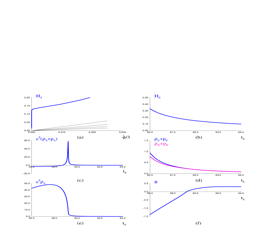
FIG. 9.: ${\cal L}_{q}=1000{\cal L}_{q}^{\phi}+1000{\cal L}_{q}^{2\phi},\Delta_{\phi}{\cal L}_{rad}=-10\dot{\phi}$. See Fig. 1 caption for details and initial conditions. We have superimposed $\rho_{R}+p_{R}$, the source quantities for the radiation onto Fig. 9d to show the onset of radiation domination.

These provide the first concrete examples of a completed graceful exit based on a classical evolution from an effective action. We have presented solutions interpolating between the inflationary $(+)$ branch to decelerated $(-)$ branch evolution in which the dilaton can be captured by a potential or stopped by radiation production. Using our analysis of the qualities and energy conditions required of sources to produce this transition we have arrived at an elusive destination.

IV Summary and Conclusions

Graceful exit transition in string cosmology is not forbidden in principle as a variety of concrete examples show explicitly. We have verified the general arguments of [7], showing that NEC violation is not just a necessary condition, but in some generic sense, also a sufficient condition. We have encountered yet another “exit problem” from a correction dominated evolution to a standard decelerated FRW evolution, which had to be overcome. We suggested that effective terms coming from higher loop corrections may do the job, and presented, for the first time, an effective Lagrangian whose equations of motion possess non-singular solutions interpolating between a $(+)$ branch vacuum and ordinary radiation dominated FRW evolution with a fixed dilaton.

The remaining questions concern whether specific string models produce coefficients of appropriate sign and size. We need to know if the one-loop terms do indeed violate NEC and whether a physical shut-off mechanism does operate in string theory. Note that the form of induced terms at one-loop is guaranteed, from general arguments, to be the one we used.

Each of our non-singular string cosmology solutions provides a detailed description of the high-curvature phase in between the dilaton-driven inflationary phase and the FRW decelerated phase (the “string phase”). In all solutions we find that a phase rich in structure appears which is much more complicated than the one postulated in [12] of constant $\dot{\phi}$ and $H_{S}$. We do not suggest taking the details of the evolution in the string phase too seriously, because the terms that determine those details have arbitrary coefficients. However, our examples could be taken as an illustration of what the real string phase may eventually look like.

Effective terms, equations of motion and their solutions

Before embarking on determining whether a definite string model has correction terms of the form required to induce the graceful exit, we have made this survey of likely forms of source terms. To do this required the variation of many forms of Lagrangian terms with many combinations of coefficients. Our interest was not in any one specific action. To make this feasible we have developed software to handle many of the aspects of the journey from action, through equations of motion and numerical integration and finally to graphical representation of the resulting dynamics in a useful form.

The core of the process is the automated derivation of the equations of motion by varying the action, in a form suitable for numerical integration. Making the process difficult was the requirement that we handle essentially any form of correction term in the action. But making the prospect easier was our specializing on homogeneous and isotropic solutions and the use of a tireless symbol manipulator, Mathematica [16]. This enables us to use an almost embarrassingly blunt approach. First we construct a matrix to represent the metric, in our case, $diag(g_{00}(t),g_{11}(t,r),g_{22}(t,r),g_{33}(t,r,\phi))$. Then we construct the tensor quantities we need in the most direct possible way. We use the metric to compute the Christoffel symbols and proceed to the Riemann tensor and contractions thereof, all of which are stored in lists. From here we compute any required geometrical scalars for the action, which all emerge in a raw form, completely in terms of $g_{00}...g_{33}$ and their various partial derivatives and any other fields.

From here we construct the $\rho$ and $p$ and other quantities by directly varying with respect to the metric fields and other quantities. Our techniques for doing this were helped greatly by study of [17]. Then we put in the cosmic time gauge choice $g_{00}=-1$ and the components of the usual FRW metric $a(t)^{2}d\Omega$ for $g_{11},g_{22},g_{33}$. Finally we replace the derivatives of $a(t)$ with their corresponding expressions in terms of the Hubble parameter $H=\dot{a}/a$.

The very crudeness of this process enhances our belief in its correctness. Other consistency checks are possible, e.g. we make the redundant check that $T^{1}_{1}=T^{2}_{2}=T^{3}_{3}$. We also verify the conservation equation (5) for these sources. They replicate many known results, e.g. the vanishing of sources from the one-loop Gauss-Bonnet combination, and we can reproduce the numerical integration of other examples in the literature. On a case by case basis we check the accuracy of numerical integrations by verifying the constraint equation (2).

Finally, we present a table of generalized sources, sufficient to construct all of the equations of motion used in this work, a generalized form of the dilaton kinetic term (45), the Ricci scalar with arbitrary dilaton dependence (50) and various $R^{2}$ combinations (54, 61 and 68). $k$ is the sign of the spatial curvature.

$${\cal{L}}_{q}^{g((\nabla\phi)^{2})} = f(\phi)g((\nabla\phi)^{2})$$ (45)

$$\rho_{q}^{g((\nabla\phi)^{2})} = {\frac{-\left(f(\phi)g((\nabla\phi)^{2})\right)}{2}}-f(\phi)g^{\prime}((\nabla\phi)^{2}){{\dot{\phi}}^{2}}$$ (46)

$$p_{q}^{g((\nabla\phi)^{2})} = {\frac{f(\phi)g((\nabla\phi)^{2})}{2}}$$ (47)

$$\Delta_{\phi}{\cal{L}}_{q}^{g((\nabla\phi)^{2})} = {\frac{g((\nabla\phi)^{2})f^{\prime}(\phi)}{2}}+3f(\phi)Hg^{\prime}((\nabla\phi)^{2})\dot{\phi}+f^{\prime}(\phi)g^{\prime}((\nabla\phi)^{2}){{\dot{\phi}}^{2}}+f(\phi)g^{\prime}((\nabla\phi)^{2})\ddot{\phi}-2f(\phi){{\dot{\phi}}^{2}}g^{\prime\prime}((\nabla\phi)^{2})\ddot{\phi}$$ (48)

$$({{(\nabla\phi)}^{2}}) = -{{\dot{\phi}}^{2}}$$ (49)

$${\cal{L}}_{q}^{R} = Rf(\phi)$$ (50)

$$\rho_{q}^{R} = {\frac{-3kf(\phi)}{{{a(t)}^{2}}}}-3f(\phi){H^{2}}-3Hf^{\prime}(\phi)\dot{\phi}$$ (51)

$$p_{q}^{R} = {\frac{kf(\phi)}{{{a(t)}^{2}}}}+3f(\phi){H^{2}}+2f(\phi)\dot{H}+2Hf^{\prime}(\phi)\dot{\phi}+{{\dot{\phi}}^{2}}f^{\prime\prime}(\phi)+f^{\prime}(\phi)\ddot{\phi}$$ (52)

$$\Delta_{\phi}{\cal{L}}_{q}^{R} = {\frac{3kf^{\prime}(\phi)}{{{a(t)}^{2}}}}+6{H^{2}}f^{\prime}(\phi)+3f^{\prime}(\phi)\dot{H}$$ (53)

$${\cal{L}}_{q}^{{R^{2}}} = R^{2}f(\phi)$$ (54)

$$\rho_{q}^{{R^{2}}} = {\frac{-18{k^{2}}f(\phi)}{{{a(t)}^{4}}}}+{\frac{36kf(\phi){H^{2}}}{{{a(t)}^{2}}}}-108f(\phi){H^{2}}\dot{H}+18f(\phi){{\dot{H}}^{2}}-{\frac{36kHf^{\prime}(\phi)\dot{\phi}}{{{a(t)}^{2}}}}-72{H^{3}}f^{\prime}(\phi)\dot{\phi}-$$ (56)

$$36Hf^{\prime}(\phi)\dot{H}\dot{\phi}-36f(\phi)H\ddot{H}$$

$$p_{q}^{{R^{2}}} = {\frac{-6{k^{2}}f(\phi)}{{{a(t)}^{4}}}}-{\frac{12kf(\phi){H^{2}}}{{{a(t)}^{2}}}}-{\frac{24kf(\phi)\dot{H}}{{{a(t)}^{2}}}}+108f(\phi){H^{2}}\dot{H}+54f(\phi){{\dot{H}}^{2}}-{\frac{24kHf^{\prime}(\phi)\dot{\phi}}{{{a(t)}^{2}}}}+48{H^{3}}f^{\prime}(\phi)\dot{\phi}+$$ (59)

$$120Hf^{\prime}(\phi)\dot{H}\dot{\phi}+{\frac{12k{{\dot{\phi}}^{2}}f^{\prime\prime}(\phi)}{{{a(t)}^{2}}}}+24{H^{2}}{{\dot{\phi}}^{2}}f^{\prime\prime}(\phi)+12\dot{H}{{\dot{\phi}}^{2}}f^{\prime\prime}(\phi)+72f(\phi)H\ddot{H}+24f^{\prime}(\phi)\dot{\phi}\ddot{H}+{\frac{12kf^{\prime}(\phi)\ddot{\phi}}{{{a(t)}^{2}}}}+$$

$$24{H^{2}}f^{\prime}(\phi)\ddot{\phi}+12f^{\prime}(\phi)\dot{H}\ddot{\phi}+12f(\phi)H^{(3)}$$

$$\Delta_{\phi}{\cal{L}}_{q}^{{R^{2}}} = {\frac{18{k^{2}}f^{\prime}(\phi)}{{{a(t)}^{4}}}}+{\frac{72k{H^{2}}f^{\prime}(\phi)}{{{a(t)}^{2}}}}+72{H^{4}}f^{\prime}(\phi)+{\frac{36kf^{\prime}(\phi)\dot{H}}{{{a(t)}^{2}}}}+72{H^{2}}f^{\prime}(\phi)\dot{H}+18f^{\prime}(\phi){{\dot{H}}^{2}}$$ (60)

$${\cal{L}}_{q}^{R^{\mu\nu}R_{\mu\nu}} = R^{\mu\nu}R_{\mu\nu}f(\phi)$$ (61)

$$\rho_{q}^{R^{\mu\nu}R_{\mu\nu}} = {\frac{-6{k^{2}}f(\phi)}{{{a(t)}^{4}}}}+{\frac{12kf(\phi){H^{2}}}{{{a(t)}^{2}}}}-36f(\phi){H^{2}}\dot{H}+6f(\phi){{\dot{H}}^{2}}-{\frac{6kHf^{\prime}(\phi)\dot{\phi}}{{{a(t)}^{2}}}}-18{H^{3}}f^{\prime}(\phi)\dot{\phi}-$$ (63)

$$12Hf^{\prime}(\phi)\dot{H}\dot{\phi}-12f(\phi)H\ddot{H}$$

$$p_{q}^{R^{\mu\nu}R_{\mu\nu}} = {\frac{-2{k^{2}}f(\phi)}{{{a(t)}^{4}}}}-{\frac{4kf(\phi){H^{2}}}{{{a(t)}^{2}}}}-{\frac{8kf(\phi)\dot{H}}{{{a(t)}^{2}}}}+36f(\phi){H^{2}}\dot{H}+18f(\phi){{\dot{H}}^{2}}-{\frac{8kHf^{\prime}(\phi)\dot{\phi}}{{{a(t)}^{2}}}}+12{H^{3}}f^{\prime}(\phi)\dot{\phi}+$$ (66)

$$36Hf^{\prime}(\phi)\dot{H}\dot{\phi}+{\frac{2k{{\dot{\phi}}^{2}}f^{\prime\prime}(\phi)}{{{a(t)}^{2}}}}+6{H^{2}}{{\dot{\phi}}^{2}}f^{\prime\prime}(\phi)+4\dot{H}{{\dot{\phi}}^{2}}f^{\prime\prime}(\phi)+24f(\phi)H\ddot{H}+8f^{\prime}(\phi)\dot{\phi}\ddot{H}+$$

$${\frac{2kf^{\prime}(\phi)\ddot{\phi}}{{{a(t)}^{2}}}}+6{H^{2}}f^{\prime}(\phi)\ddot{\phi}+4f^{\prime}(\phi)\dot{H}\ddot{\phi}+4f(\phi)H^{(3)}$$

$$\Delta_{\phi}{\cal{L}}_{q}^{R^{\mu\nu}R_{\mu\nu}} = {\frac{6{k^{2}}f^{\prime}(\phi)}{{{a(t)}^{4}}}}+{\frac{18k{H^{2}}f^{\prime}(\phi)}{{{a(t)}^{2}}}}+18{H^{4}}f^{\prime}(\phi)+{\frac{6kf^{\prime}(\phi)\dot{H}}{{{a(t)}^{2}}}}+18{H^{2}}f^{\prime}(\phi)\dot{H}+6f^{\prime}(\phi){{\dot{H}}^{2}}$$ (67)

$${\cal{L}}_{q}^{R^{\mu\nu\sigma\lambda}R_{\mu\nu\sigma\lambda}} = R^{\mu\nu\sigma\lambda}R_{\mu\nu\sigma\lambda}f(\phi)$$ (68)

$$\rho_{q}^{R^{\mu\nu\sigma\lambda}R_{\mu\nu\sigma\lambda}} = {\frac{-6{k^{2}}f(\phi)}{{{a(t)}^{4}}}}+{\frac{12kf(\phi){H^{2}}}{{{a(t)}^{2}}}}-36f(\phi){H^{2}}\dot{H}+6f(\phi){{\dot{H}}^{2}}-12{H^{3}}f^{\prime}(\phi)\dot{\phi}-12Hf^{\prime}(\phi)\dot{H}\dot{\phi}-12f(\phi)H\ddot{H}$$ (69)

$$p_{q}^{R^{\mu\nu\sigma\lambda}R_{\mu\nu\sigma\lambda}} = {\frac{-2{k^{2}}f(\phi)}{{{a(t)}^{4}}}}-{\frac{4kf(\phi){H^{2}}}{{{a(t)}^{2}}}}-{\frac{8kf(\phi)\dot{H}}{{{a(t)}^{2}}}}+36f(\phi){H^{2}}\dot{H}+18f(\phi){{\dot{H}}^{2}}-{\frac{8kHf^{\prime}(\phi)\dot{\phi}}{{{a(t)}^{2}}}}+8{H^{3}}f^{\prime}(\phi)\dot{\phi}+$$ (72)

$$32Hf^{\prime}(\phi)\dot{H}\dot{\phi}+4{H^{2}}{{\dot{\phi}}^{2}}f^{\prime\prime}(\phi)+4\dot{H}{{\dot{\phi}}^{2}}f^{\prime\prime}(\phi)+24f(\phi)H\ddot{H}+8f^{\prime}(\phi)\dot{\phi}\ddot{H}+4{H^{2}}f^{\prime}(\phi)\ddot{\phi}+$$

$$4f^{\prime}(\phi)\dot{H}\ddot{\phi}+4f(\phi)H^{(3)}$$

$$\Delta_{\phi}{\cal{L}}_{q}^{R^{\mu\nu\sigma\lambda}R_{\mu\nu\sigma\lambda}} = {\frac{6{k^{2}}f^{\prime}(\phi)}{{{a(t)}^{4}}}}+{\frac{12k{H^{2}}f^{\prime}(\phi)}{{{a(t)}^{2}}}}+12{H^{4}}f^{\prime}(\phi)+12{H^{2}}f^{\prime}(\phi)\dot{H}+6f^{\prime}(\phi){{\dot{H}}^{2}}$$ (73)

REFERENCES

- [1] G. Veneziano, Phys. Lett. B265 (1991) 287.
- [2] M. Gasperini and G. Veneziano, Astropart. Phys. 1 (1993) 317.
-
[3]
K.A. Meissner and G. Veneziano, Phys. Lett. B267 (1991) 33;
K.A. Meissner and G. Veneziano, Mod. Phys. Lett. A6 (1991) 3397;
A. Sen, Phys. Lett. B271 (1991) 295;
M. Gasperini and G. Veneziano, Phys. Lett. B277 (1992) 256;
K.A. Meissner, Phys. Lett. B392 (1997) 298. - [4] A.A. Tseytlin and C. Vafa, Nucl. Phys. B372 (1992) 443.
- [5] R. Brustein and G. Veneziano, Phys. Lett. B329 (1994) 429.
-
[6]
G. Veneziano, hep-th/9703150;
E. Weinberg and M. Turner, hep-th/9705035;
M. Maggiore and R. Sturani, hep-th/9706053;
A. Bounanno, K. A. Meissner, G. Veneziano and C. Ungarelli, hep-th/9706221. - [7] R. Brustein and R. Madden, hep-th/9702043.
-
[8]
E.J. Copeland, A. Lahiri and D. Wands, Phys. Rev. D50 (1994) 4868;
J. Levin, Phys. Rev. D51 (1995) 462;
J. Levin, Phys. Rev. D51 (1995) 1536;
E.J. Copeland, A. Lahiri and D. Wands, Phys. Rev. D51 (1995) 1569;
J. Levin, Phys. Lett. B343 (1995) 69;
N. Kaloper, R. Madden and K.A. Olive, Phys. Lett. B371 (1996) 34;
R. Easther, K. Maeda and D. Wands, Phys. Rev. D53 (1996) 4247;
I. Antoniadis, J. Rizos and K. Tamvakis, Nucl. Phys. B415 (1993) 497;
R. Easther and K. Maeda, Phys. Rev. D54 (1996) 7252;
J.E. Lidsey, Phys. Rev. D55 (1997) 3303;
N. Kaloper, Phys. Rev. DD55 (1997) 3394;
J.E. Lidsey, gr-qc/9609063;
R. Poppe and S. Schwager, Phys. Lett. B393 (1997) 51;
A. Lukas, Burt A. Ovrut and D. Waldram, Nucl. Phys. B495 (1997) 365;
S. K. Rama, hep-th/9701154;
S. Bose and S. Kar, hep-th/9705061;
W. T. Kim and M. S. Yoon, hep-th/9704115;
W. T. Kim and M. S. Yoon, hep-th/9706154. -
[9]
M. Gasperini, J. Maharana and G. Veneziano, Nucl. Phys. B472 (1996) 349;
A. Lukas and R. Poppe, Mod. Phys. Lett. A12 (1997) 597;
S.-J. Rey, Phys. Rev. Lett. 77 (1996) 1929;
M. Gasperini and G. Veneziano, Phys. Lett. B387 (1996) 715;
M. P. Dabrowski and C. Kiefer, Phys. Lett. B397 (1997) 185;
J. Maharana, S. Mukherji and S. Panda, Mod. Phys. Lett. A12 (1997) 447;
A. Buonanno, M. Gasperini, M. Maggiore and C. Ungarelli, Class.Quant.Grav.14 (1997) L97-L103;
Z. Lalak and R. Poppe, gr-qc/9704083. - [10] M. Gasperini, M. Maggiore and G. Veneziano, Nucl. Phys. B494 (1997) 315.
- [11] N. Kaloper, R. Madden and K.A. Olive, Nucl. Phys. B452 (1995) 677.
- [12] R. Brustein, M. Gasperini, M. Giovannini and G. Veneziano, Phys. Lett. B361 (1995) 45.
-
[13]
S. W. Hawking and G. F. R. Ellis, The large scale structure of space-time,
Cambridge University Press, Cambridge, England, 1973;
A more recent clear summary appeared in S. W. Hawking, hep-th/9409195. - [14] M. Gasperini and G. Veneziano, Mod. Phys. Lett. A8 (1993) 3701.
- [15] E. Flanagan and R. Wald, Phys. Rev. D54 (1996) 6233;
- [16] S. Wolfram, Mathematica, a System for Doing Mathematics by Computer, (Addison-Wesley Publishing Company, Inc. 1991.
-
[17]
Y. He, Mathematica Package “VariationalMethods”,
Copyright 1992-1996, Wolfram Research, Inc.