SU(N) Monopoles and Platonic Symmetry

Abstract

We discuss the ADHMN construction for $SU(N)$ monopoles and show that a particular simplification arises in studying charge $N-1$ monopoles with minimal symmetry breaking. Using this we construct families of tetrahedrally symmetric $SU(4)$ and $SU(5)$ monopoles. In the moduli space approximation, the $SU(4)$ one-parameter family describes a novel dynamics where the monopoles never separate, but rather, a tetrahedron deforms to its dual. We find a two-parameter family of $SU(5)$ tetrahedral monopoles and compute some geodesics in this submanifold numerically. The dynamics is rich, with the monopoles scattering either once or twice through octahedrally symmetric configurations.

PACS: 11.27.+d, 11.15.-q

I Introduction

Bogomolny-Prasad-Sommerfield monopoles are static solitons occurring in certain (3+1)-dimensional gauge field theories. They have attracted interest continually since they were discovered over two decades ago. The simplest BPS monopoles are $SU(2)$ monopoles, which have an associated integer referred to as the topological charge. Monopoles with topological charge $k$ are called $k$-monopoles, and their total energy is proportional to $k$. For any given $k$ there are $k$-monopole solutions which resemble $k$ well-separated 1-monopoles.

It is interesting, but often difficult, to examine monopoles associated with gauge groups larger than $SU(2)$. Such monopoles have features not found in the $SU(2)$ case, for example, the existence of spherically symmetric multi-monopoles [1].

There is a powerful approach to monopoles; the ADHMN construction. To perform this construction a nonlinear differential equation, called the Nahm equation, must be solved and its solution, the Nahm data, used to define a linear ordinary differential equation. This linear equation, which we shall refer to as the ADHMN construction equation, must then be solved. Its solutions yield the fields via an integration procedure. Recently Platonic symmetries have been exploited to construct Nahm data and these symmetric Nahm data have been used to examine some particular examples of $SU(2)$ monopoles. In this paper we discuss two cases where the same Platonic Nahm data, slightly modified, can be used to study monopoles associated with larger gauge groups.

Section II is an introduction to $SU(N)$ Nahm data and monopoles. We show that for minimal symmetry breaking the Nahm data for some multi-monopoles is simpler than the corresponding $SU(2)$ Nahm data. This allows us, in a simple way, to modify known $SU(2)$ Nahm data so that it is $SU(N)$ Nahm data. It is possible to use $SU(2)$ Nahm data to produce $SU(2)$ monopoles embedded in an $SU(N)$ theory. Such embedded monopoles behave like $SU(2)$ monopoles. The modification we consider is more radical than a simple embedding and the corresponding monopoles behave quite unlike the way $SU(2)$ monopoles do.

In Section III we use charge three Nahm data with tetrahedral symmetry to construct a one-parameter family of $SU(4)$ monopoles with tetrahedral symmetry. The dynamics of slow moving monopoles is approximated by geodesic motion in the moduli space of solutions [2]. Since the one-parameter family of solutions described in Section III is the fixed point set of the action of the tetrahedral group, it must be a geodesic. Thus the one-parameter family described in Section III is an example of a pathological scattering process in which the monopole never separates into distinct objects.

In Section IV we use charge four Nahm data with tetrahedral symmetry to construct a two-parameter family of $SU(5)$ monopoles with tetrahedral symmetry. This two-parameter family is totally geodesic in the whole moduli space. Under the assumption that the transformation between the metric on the space of Nahm data and the metric on the moduli space of monopoles is an isometry, we undertake a numerical study of the low energy dynamics of $SU(5)$ tetrahedral monopoles. We find an exotic dynamics involving both single and double scatterings through configurations with octahedral symmetry.

II Monopoles and Nahm data

BPS $SU(N)$ monopoles are topological solitons in an $SU(N)$ Yang-Mills-Higgs gauge theory with no Higgs self-coupling. They are finite energy solutions to the Bogomolny equation

$$D_{i}\Phi=-\frac{1}{2}\epsilon_{ijk}F_{jk}$$ (2.1)

where $D_{i}=\frac{\partial}{\partial x_{i}}+[A_{i},$  is the covariant derivative with $A_{i}$ an su(N)-valued gauge potential and $F_{jk}$ the gauge field. $\Phi$ is an su(N)-valued scalar field, called the Higgs field. Non-trivial asymptotic conditions are imposed on the Higgs field, which are responsible for the existence of topological soliton solutions to the theory. It is required that, as $r=|{\bf x}|$ approaches infinity, $\Phi$ takes values in the gauge orbit of the matrix

$$M=i\,\mbox{diag}\,(\mu_{1},\mu_{2},\ldots,\mu_{N}).$$ (2.2)

By convention it is assumed that $\mu_{1}\leq\mu_{2}\leq\ldots\leq\mu_{N}$. Since $\Phi$ is traceless $\mu_{1}+\mu_{2}+\ldots+\mu_{N}=0$. This $M$ is the vacuum expectation value for $\Phi$ and the symmetry group of $M$ under gauge transformation is called the residual, or unbroken, symmetry group. Thus, for example, if all the $\mu_{p}$ are different the residual symmetry group is the maximal torus $U(1)^{N-1}$. This is known as maximal, or generic, symmetry breaking. The soliton solutions are associated with $N-1$ integers; this is because the boundary condition on $\Phi$ implies a map, $\Phi_{\infty}$, from the large sphere at infinity into the quotient group

$$\Phi_{\infty}:S^{2}\rightarrow\mbox{orbit}_{SU(N)}M\ =SU(N)/U(1)^{N-1}$$ (2.3)

and

$$\pi_{2}\left(SU(N)/U(1)^{N-1}\right)=\pi_{1}(U(1)^{N-1})=\hbox{\upright\hbox to0.0pt{\sans Z\hss}\kern 2.7pt{\sans Z}}^{N-1}.$$ (2.4)

In contrast, this paper concerns the minimal symmetry breaking case, in which all but one of the $\mu_{p}$ are identical, so the residual symmetry group is $U(N-1)$. It is convenient to choose $\mu_{1}=-(N-1)$ and $\mu_{p}=1$ for $p=2\ldots N$. Since

$$\pi_{2}\left(SU(N)/U(N-1)\right)=\hbox{\upright\hbox to0.0pt{\sans Z\hss}\kern 2.7pt{\sans Z}}$$ (2.5)

there is only one topological integer associated with solutions. Nonetheless, a given solution has $N-1$ integers associated with it, these arise in the following way; careful analysis of the boundary conditions indicates that there is a choice of gauge such that the Higgs field for large $r$, in a given direction, is given by

$$\Phi(r)=i\,\mbox{diag}\,(\mu_{1},\mu_{2},\ldots,\mu_{N})-\frac{i}{2r}\,\mbox{diag}\,(k_{1},k_{2},\ldots,k_{N})+O(r^{-2}).$$ (2.6)

In the maximal symmetry breaking case the topological charges are given by

$$m_{p}=\sum_{q=1}^{p}k_{q}.$$ (2.7)

In the case of minimal symmetry breaking only the first of these numbers, $m_{1}$, is a topological charge. Nonetheless, the remaining $m_{p}$ constitute an integer characterization of a solution. This characterization is gauge invariant up to reordering of the integers $k_{p}$. The $m_{p}$ are known as magnetic weights, with the matrix $\mbox{diag}\,(k_{1},k_{2},\ldots,k_{N})$ often called the charge matrix.

There are some obvious ways of embedding $su(2)$ in $su(N)$, for example,

$$\left(\begin{array}[]{cc}\alpha&\beta\\ -\bar{\beta}&-\alpha\end{array}\right)\hookrightarrow\left(\begin{array}[]{ccccc}\ddots&&&&\\ &\alpha&\ldots&\beta&\\ &\vdots&\ddots&\vdots&\\ &-\bar{\beta}&\ldots&-\alpha&\\ &&&&\ddots\end{array}\right).$$ (2.8)

Important $SU(N)$ monopoles can be produced by embedding the $SU(2)$ 1-monopole fields, which are known $su(2)$-valued fields, in $su(N)$. Some care must be taken in producing these embedded monopoles to ensure that the asymptotic behaviour is correct; the $SU(2)$ monopole may need to be scaled and it may be necessary to add a constant diagonal field beyond the plain embedding described by (2.8), details may be found in [3, 4]. Obviously there is an embedding of the form (2.8) for each choice of two columns in the target matrix. The embedded 1-monopoles have a single $k_{p}=1$ and another $k_{p}=-1$, the rest are zero. The choice of columns for the embedding dictates which two $k_{p}$ are non-zero. Recall that in the case of minimal symmetry breaking the choice of order of the $k_{p}$ is a gauge choice. In fact, in the case of minimal symmetry breaking, the embedded 1-monopole is unique up to position and gauge transformation. Solutions with $k_{1}=k$ have $k$ times the energy of this basic solution and so it is reasonable to call these $k_{p}=k$ monopoles $k$-monopoles. There are of course different types of such $k$-monopoles corresponding to different magnetic weights.

Consider $SU(3)$ monopoles with minimal symmetry breaking. For $k=2$ there are two distinct types of monopoles, those with $m_{2}=0$ and those with $m_{2}=1$. The $m_{2}=2$ case is equivalent to the $m_{2}=0$ case; $m_{2}$ can be changed from 0 to 2 by reordering $k_{2}$ and $k_{3}$. If $m_{2}=0$ the monopoles are all embeddings of $su(2)$ 2-monopoles and this case is not interesting as an example of $su(3)$ 2-monopoles. The $m_{2}=1$ case has been studied by Dancer [5] and by Dancer and Leese [6], by considering Nahm data.

There is an equivalence between Nahm data and BPS monopoles. In the case of $SU(N)$ monopoles the Nahm data are triplets of anti-hermitian matrix functions $(T_{1},T_{2},T_{3})$ of $s$ over the intervals $(\mu_{p},\mu_{p+1})$. The size of the matrices depends on the corresponding values of $m_{p}$; the matrices $(T_{1},T_{2},T_{3})$ are $m_{p}\times m_{p}$ matrices in the interval $(\mu_{p},\mu_{p+1})$. They are required to be non-singular in each region and to satisfy the Nahm equation

$$\frac{dT_{i}}{ds}=\frac{1}{2}\epsilon_{ijk}[T_{j},T_{k}].$$ (2.9)

There are complicated boundary conditions prescribed between the Nahm data in abutting intervals, which are detailed in Nahm’s original paper [7]. We will follow Hurtubise and Murray’s formulation of the Nahm data boundary conditions for distinct $\mu_{p}$ [8] and then take the limit of coincident $\mu_{p}$ to describe the minimal symmetry breaking case.

For ease of notation we shall describe the case where $m_{p-1}\geq m_{p}$ (ie. $k_{p}\leq 0$ for $p>1$) since a similar result holds after a reordering if this is not satisfied.

Monopoles are constructed from their corresponding Nahm data by first solving a first order differential equation in which the Nahm data appear as coefficients. This is called the ADHMN construction equation. This choice affects the order of the $k_{p}$. Rather than describe it in full generality, it will be described below in the particular form required. The matching and boundary conditions on Nahm data are designed to ensure that the ADHMN construction equation has the correct number of solutions required to yield the correct type of monopole fields. Define the function

$$k(s)=\sum_{p=1}^{N}k_{p}\,\theta(s-\mu_{p})$$ (2.10)

where $\theta(s)$ is the usual Heaviside function. In the interval $(\mu_{p},\mu_{p+1})$ $k(s)=m_{p}$. It is a rectilinear skyline whose shape depends on the charge matrix of the corresponding monopole. If $k(s)$ near $\mu_{p}$ is

then as $s$ approaches $\mu_{p}$ from below we require

$$T_{i}(s)=\left(\begin{array}[]{cc}\frac{1}{z}R_{i}+O(1)&O(z^{(|k_{p}|-1)/2})\\ O(z^{(|k_{p}|-1)/2})&T_{i}^{\prime}+O(z)\end{array}\right)$$ (2.11)

where $z=s-\mu_{p}$ and where

$$T_{i}(s)=T_{i}^{\prime}+O(z)$$ (2.12)

as $s$ approaches $\mu_{p}$ from above.

It follows from the Nahm equation (2.9) that the $|k_{p}|\times|k_{p}|$ residue matrices $(R_{1},R_{2},R_{3})$ in (2.11) form a representation of $su(2)$. The boundary conditions require that this representation is the unique irreducible $|k_{p}|$-dimensional representation of $su(2)$.

In summary, at the boundary between two abutting intervals, if the Nahm matrices are $m_{p-1}\times m_{p-1}$ on the left and $m_{p}\times m_{p}$ on the right an $m_{p}\times m_{p}$ block continues through the boundary and there is an $(m_{p-1}-m_{p})\times(m_{p-1}-m_{p})$ block simple pole whose residues form an irreducible representation of $su(2)$. The boundary conditions for $m_{p-1}=m_{p}$ are given in, for example, [8]. While these boundary conditions are involved, their function is simply one of limiting the number of solutions to the ADHMN construction equation.

The 1-dimensional representations of $su(2)$ are trivial. Thus, if $k_{p}=-1$ for all $p>1$, $k(s)$ is

and the Nahm data has only one pole, it is at $s=\mu_{1}$. It seems reasonable to suppose that this result holds in the limit of coincident $\mu_{p}$. Thus, if we fix $\mu_{1}=-(N-1)$ and $\mu_{p\not=1}=1$, we expect that the $N\times N$ Nahm data whose sole pole is at $s=-(N-1)$, satisfying the Nahm equations and having acceptable residues, are the Nahm data of $SU(N)$ monopoles with minimal symmetry breaking. For this to be the case it is only required that the ADHMN construction equation have the correct number of solutions over the interval. This index calculation is easily performed using the methods of [8]. The topological charge of the corresponding monopole solution is, of necessity, $k_{1}=N-1$, since the $k_{p}$ must add to zero. The magnetic weights are each one less than the proceeding one. We say that the magnetic weights are distinct. It has recently been proven by Nakajima that all monopoles of this type can be constructed from the described Nahm data[9].

The Nahm data for $su(2)$ $k$-monopoles are $k\times k$ anti-hermitian matrix solutions of the Nahm equation. They have poles at $s=-1$ and $s=1$. It is obvious that this Nahm data,

can be used to generate Nahm data for $SU(k+1)$ $k$-monopoles with distinct weights

In examples where the charge $k$ $SU(2)$ data is known, the $SU(k+1)$ data is generated by a translation and rescaling of $s$ so that a pole occurs at $s=\mu_{1}$ but the second pole is moved outside the interval $s\in[\mu_{1},\mu_{N}]$ ie. it is lost from the Nahm data. The 2-monopole Nahm data is known exactly, and was used by Dancer in [5] to construct $SU(3)$ monopoles. This is the simplest application of the above procedure. Platonic symmetry groups have previously been used to derive higher charge Nahm data, and in this paper we discuss the corresponding $SU(k+1)$ monopoles.

III SU(4) monopoles with tetrahedral symmetry

In the previous Section we discussed the Nahm data for $SU(k+1)$ monopoles with minimal symmetry breaking, charge $k$ and distinct magnetic weights. For the remainder of the paper it will be convenient to perform a translation $s\mapsto s-\mu_{1}$, so that a pole in the Nahm data always occurs at $s=0$. In this Section we describe some aspects of the the ADHMN construction, which calculates the monopole fields $(\Phi,A_{i})$ from the Nahm data. We then go on to apply this construction to obtain a one-parameter family of monopoles with $k=3$, which have tetrahedral symmetry.

Given Nahm data $(T_{1},T_{2},T_{3})$ for a $k$-monopole we must solve the ADHMN construction equation, for $s\in[0,k+1]$,

$$({{\upright\hbox to0.0pt{1\hss}\kern 2.0pt1}}_{2k}\frac{d}{ds}+{{\upright\hbox to0.0pt{1\hss}\kern 2.0pt1}}_{k}\otimes x_{j}\sigma_{j}+iT_{j}\otimes\sigma_{j}){\bf v}=0$$ (3.1)

for the complex $2k$-vector ${\bf v}(s)$, where ${\upright\hbox to0.0pt{1\hss}\kern 2.0pt1}_{k}$ denotes the $k\times k$ identity matrix, $\sigma_{j}$ are the Pauli matrices and ${\bf x}=(x_{1},x_{2},x_{3})$ is the point in space at which the monopole fields are to be calculated. Introducing the inner product

$$\langle{\bf v}_{1},{\bf v}_{2}\rangle=\int_{0}^{k+1}{\bf v}_{1}^{\dagger}{\bf v}_{2}\ ds$$ (3.2)

then the solutions of (3.1) which we require are those which are normalizable with respect to (3.2). It can be shown that the space of normalizable solutions to (3.1) has (complex) dimension $k+1$. If $\widehat{\bf v}_{1},..,\widehat{\bf v}_{k+1}$ is an orthonormal basis for this space then the $ij$th matrix element, $(\Phi)_{ij}$, of the Higgs field is given by

$$(\Phi)_{ij}=i\langle(s-k)\widehat{\bf v}_{i},\widehat{\bf v}_{j}\rangle$$ (3.3)

A similar expression exists for the gauge potential, but the energy density, ${\cal E}$, may be computed without calculating the gauge potential by using the formula

$${\cal E}=\bigtriangleup\mbox{tr}(\Phi^{2})$$ (3.4)

where $\bigtriangleup$ denotes the Laplacian on IR³.

For most of the examples considered in this paper the Nahm data is sufficiently complicated that the matrix linear differential equation (3.1) can not be solved analytically in closed form. In these cases we use a numerical implementation of the ADHMN construction which involves solving the ordinary differential equations using a standard fourth order Runge-Kutta method. The numerical implementation is similar to that introduced by the authors in [10], but is simplified by the fact that the Nahm data we consider here has a pole at only one end of the $s$ interval. This eliminates the need for the shooting part of the numerical algorithm described in [10].

In references [11, 10, 12] it is explained how Platonic symmetry (that is, tetrahedral, octahedral or icosahedral symmetry) may be applied to Nahm data for $SU(2)$ monopoles of charge $k$. We use these, as explained in the previous Section, to easily obtain the solutions to Nahm’s equation for $SU(k+1)$ monopoles.

From [10] we have that the Nahm data for tetrahedrally symmetric monopoles with $k=3$ has the form

$$T_{1}=\left[\begin{array}[]{ccc}0&0&0\\ 0&0&-z\\ 0&\bar{z}&0\end{array}\right]\;\;T_{2}=\left[\begin{array}[]{ccc}0&0&-\bar{z}\\ 0&0&0\\ z&0&0\end{array}\right]\;\;T_{3}=\left[\begin{array}[]{ccc}0&z&0\\ -\bar{z}&0&0\\ 0&0&0\end{array}\right]$$ (3.5)

where

$$z=\frac{\omega\wp^{\prime}(\omega s)}{2\wp(\omega s)}+\frac{\sqrt{3}\omega}{\wp(\omega s)}\mbox{ , }\;\;\omega=e^{i\pi/6}\kappa$$ (3.6)

and $\wp$ is the Weierstrass function satisfying

$$\wp^{\prime 2}=4\wp^{3}-4$$ (3.7)

where ^′ denotes differentiation with respect to the argument.

For $SU(2)$ monopoles the boundary condition requires that the Nahm data has a simple pole at $s=2$ which determines $\kappa$ to be

$$\pm\kappa=\kappa_{0}=\frac{\Gamma(1/6)\Gamma(1/3)}{12\sqrt{\pi}}.$$ (3.8)

For $SU(4)$ monopoles the corresponding boundary condition is less restrictive, namely that we require the Nahm data to have no poles for $s\in(0,4]$. Given the $SU(2)$ result this implies that $\kappa$ must satisfy the condition

$$-\kappa_{0}/2<\kappa<\kappa_{0}/2.$$ (3.9)

It is a simple task to show that the remaining requirements for Nahm data are satisfied, and hence we have proved the existence of a one-parameter family of $SU(4)$ monopoles with tetrahedral symmetry. The one-parameter family is given by $\kappa$ in the above interval and the corresponding family of spectral curves is

$$\eta^{3}+i36\kappa^{3}\zeta(\zeta^{4}-1)=0.$$ (3.10)

Note that $\kappa=0$ gives the spectral curve $\eta^{3}=0$, which is the spectral curve of a 3-monopole with spherical symmetry. Such a spherically symmetric monopole was constructed several years ago [1] by using a spherically symmetric ansatz in the field equations. We shall now see how this solution arises in the ADHMN construction by explicitly calculating the Higgs field in this case.

Taking the limit $\kappa\rightarrow 0$ and using the property that

$$\wp(u)\sim u^{-2}\hskip 10.0pt\mbox{as}\hskip 10.0ptu\rightarrow 0$$ (3.11)

gives

$$z=-1/s$$ (3.12)

in this limit.

Since the monopole with this Nahm data is spherically symmetric, we only need to constructing the Higgs field along an axis. Setting $(x_{1},x_{2},x_{3})=(0,0,r)$ the linear equation (3.1) becomes

$$\frac{d{\bf v}}{ds}+\left[\begin{array}[]{cccccc}(r-1/s)&0&0&0&0&0\\ 0&-(r-1/s)&-\sqrt{2}/s&0&0&0\\ 0&-\sqrt{2}/s&r&0&0&0\\ 0&0&0&-r&-\sqrt{2}/s&0\\ 0&0&0&-\sqrt{2}/s&(r+1/s)&0\\ 0&0&0&0&0&-(r+1/s)\end{array}\right]{\bf v}=0.$$ (3.13)

Clearly the first and last components of ${\bf v}$ decouple and are elementary to solve. The remaining four equations may be decoupled into two pairs, which can then be converted into two second order equations and solved by a Laplace transform. The full regular solution is

$${\bf v}=\left[\begin{array}[]{c}c_{1}se^{-rs}\\ \\ c_{2}\sqrt{2}(\frac{\cosh(rs)}{rs}-\frac{\sinh(rs)}{r^{2}s^{2}})\\ \\ c_{2}(\frac{\sinh(rs)}{r^{2}s^{2}}-e^{-rs}(1+\frac{1}{rs}))\\ \\ c_{3}(-\frac{\sinh(rs)}{r^{2}s^{2}}-e^{rs}(1-\frac{1}{rs}))\\ \\ -c_{3}\sqrt{2}(\frac{\cosh(rs)}{rs}-\frac{\sinh(rs)}{r^{2}s^{2}})\\ \\ c_{4}se^{rs}\end{array}\right]$$ (3.14)

where $c_{1},c_{2},c_{3},c_{4}$ are arbitrary constants. If we select the orthonormal basis $\widehat{\bf v}_{i}$ where $\widehat{\bf v}_{i}$ has only $c_{i}$ non-zero, then the Higgs field will be diagonal. Performing the required integrals (3.3) gives the result

$$(\Phi)_{11} = -i\ \frac{6r-3+e^{-8r}(64r^{3}+48r^{2}+18r+3)}{2r(1-e^{-8r}(32r^{2}+8r+1))}$$ (3.15)

$$(\Phi)_{33} = i\ \frac{e^{8r}(-4r+3)-384r^{3}+64r^{2}-40r-6+e^{-8r}(128r^{3}+128r^{2}+44r+3)}{e^{8r}(-4r+1)+128r^{3}-8r-2+e^{-8r}(128r^{3}+64r^{2}+12r+1)}$$ (3.16)

with $(\Phi)_{22}$ and $(\Phi)_{44}$ obtained by the replacement $r\mapsto-r$ in $(\Phi)_{11}$ and $(\Phi)_{33}$ respectively. It is a simple task to verify that indeed this solution has the correct asymptotic behaviour ie.

$$\Phi\rightarrow i\mbox{diag}(-3,1,1,1)\hskip 28.45274pt\mbox{as}\hskip 28.45274ptr\rightarrow\infty.$$ (3.17)

To compute the Higgs field for non-zero values of $\kappa$ is a much more difficult task, since all the components of the vector ${\bf v}$ become coupled together. Thus we turn to the numerical implementation of the ADHMN construction. In Figure 1 we display the results in the form of three dimensional plots of surfaces of constant energy density for the values $\kappa/\kappa_{0}=-0.25,-0.10,0.00,+0.10,+0.25$. As the parameter $\kappa$ increases from zero, the spherical monopole deforms into a tetrahedral monopole. As $\kappa\rightarrow\pm\kappa_{0}/2$, the monopole approaches the embedded $SU(2)$ tetrahedral 3-monopole asymptotically. In fact, even for the value $\kappa=-\kappa_{0}/4$ (Figure 1.1) the energy density looks very similar to that of the $SU(2)$ tetrahedral 3-monopole [10]. Note that changing the sign of $\kappa$ gives a monopole corresponding to the dual tetrahedron.

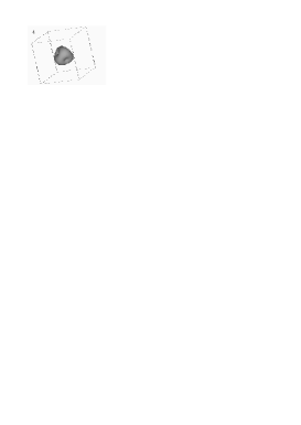
FIG. 1.: Tetrahedral scattering of an $SU(4)$ 3-monopole.

In the moduli space approximation [2] the dynamics of $k$ monopoles is approximated by geodesic motion on the $k$-monopole moduli space ${\cal M}_{k}$. From the spectral curve approach it is clear that, having fixed an orientation and centre of mass, we have constructed the unique one-parameter family of tetrahedrally symmetric $SU(4)$ 3-monopoles. Since the fixed point set of a group action gives a totally geodesic submanifold, this one-parameter family is a geodesic in ${\cal M}_{3}$. Hence, within the moduli space approximation, this family of monopoles may be interpreted as describing the low energy dynamics of three deforming monopoles. Using this interpretation we see from Figure 1 that during the course of the motion a tetrahedron gets smoothed out into a sphere which then deforms back into the dual tetrahedron. This gives an example of dynamics in which the monopoles never become separated.

It is known in the case of $SU(2)$ monopoles that there are closed geodesics [13, 14, 15]. In the geodesics approximation such geodesics correspond to periodic monopole motions during which the monopoles never separate. That is not the case here, here the motion is not periodic and the geodesic is not closed; it runs between points on the asymptotic boundary of the moduli space which do not correspond to separated monopoles.

Obviously the method applied in this Section to tetrahedral $SU(4)$ 3-monopoles can easily be carried over to construct $SU(k+1)$ $k$-monopoles, given the Nahm data for an $SU(2)$ $k$-monopole. In general, given a $p$-dimensional family of $SU(2)$ monopoles there will be a corresponding $(p+1)$-dimensional family of $SU(k+1)$ monopoles. Thus, for example, it is a simple task to construct the Nahm data for the one-parameter family of octahedrally symmetric $SU(5)$ 4-monopoles which derive from the unique octahedrally symmetric $SU(2)$ 4-monopole [11]. However, it is more interesting to consider geodesic motion in the two-dimensional moduli space of $SU(k+1)$ monopoles derived from a one-parameter family of $SU(2)$ monopoles corresponding to a geodesic in the $SU(2)$ moduli space. Physically, this will allow us to examine how the dynamics of $SU(k+1)$ monopoles compares with the dynamics of $SU(2)$ monopoles. We shall do this in the following Section, for the case of $SU(5)$ 4-monopoles with tetrahedral symmetry.

IV SU(5) monopoles with tetrahedral symmetry

After fixing the orientation and centre of mass, there is a one-parameter family of tetrahedrally symmetric charge four $SU(2)$ monopoles [10]. The associated Nahm data takes the form

$$T_{i}(s)=x(s)X_{i}+y(s)Y_{i}+z(s)Z_{i}\hskip 20.0pti=1,2,3$$ (4.1)

where the tetrahedrally symmetric Nahm triplets are

$$(X_{1}+iX_{2},X_{3}) = \left(2\left[{\begin{array}[]{cccc}0&0&0&0\\ -\sqrt{3}&0&0&0\\ 0&-2&0&0\\ 0&0&-\sqrt{3}&0\end{array}}\right],\left[{\begin{array}[]{cccc}3i&0&0&0\\ 0&i&0&0\\ 0&0&-i&0\\ 0&0&0&-3i\end{array}}\right]\right)$$ (4.10)

$$(Y_{1}+iY_{2},Y_{3}) = 4\left(\left[{\begin{array}[]{cccc}0&0&0&-5\\ \sqrt{3}&0&0&0\\ 0&-3&0&0\\ 0&0&\sqrt{3}&0\end{array}}\right],\left[{\begin{array}[]{cccc}i&0&0&0\\ 0&-3i&0&0\\ 0&0&3i&0\\ 0&0&0&-i\end{array}}\right]\right)$$ (4.19)

$$(Z_{1}+iZ_{2},Z_{3}) = \sqrt{3}\left(2\left[{\begin{array}[]{cccc}0&i&0&0\\ 0&0&0&0\\ 0&0&0&-i\\ 0&0&0&0\end{array}}\right],\left[{\begin{array}[]{cccc}0&0&1&0\\ 0&0&0&1\\ -1&0&0&0\\ 0&-1&0&0\end{array}}\right]\right)$$ (4.28)

The reduced equations for the three real functions $x,y,z$ can be solved to yield

$$x(s) = \frac{\kappa}{5}\left(-2\sqrt{\wp(\kappa s)}+\frac{1}{4}\frac{\wp^{\prime}(\kappa s)}{\wp(\kappa s)}\right)$$ (4.29)

$$y(s) = \frac{\kappa}{20}\left(\sqrt{\wp(\kappa s)}+\frac{1}{2}\frac{\wp^{\prime}(\kappa s)}{\wp(\kappa s)}\right)$$ (4.30)

$$z(s) = \frac{a\kappa}{2\wp(\kappa s)}.$$ (4.31)

Here $\wp$ is the Weierstrass function satisfying

$$\wp^{\prime 2}=4\wp^{3}-4\wp+12a^{2}$$ (4.32)

with prime denoting differentiation with respect to the argument.

The spectral curve for tetrahedrally symmetric 4-monopoles has the form

$$\eta^{4}+i\alpha\eta\zeta(\zeta^{4}-1)+\beta^{2}(\zeta^{8}+14\zeta^{4}+1)=0$$ (4.33)

where $\alpha$ and $\beta$ are real constants. The relation between these constants and those appearing in the above Nahm data is given by

$$\alpha=36a\kappa^{3},\hskip 28.45274pt\beta^{2}=3\kappa^{4}.$$ (4.34)

In the $SU(2)$ case, the requirement that the Nahm data has a second pole at $s=2$ means that $\kappa$ must be taken to be half the real period of the elliptic function (4.32). Thus, $\kappa$ is determined given the parameter $a$, and we have the required one-parameter family. Furthermore, $a$ is restricted to lie in the interval $a\in(-a_{c},a_{c})$, with $a_{c}=3^{-5/4}\sqrt{2}$. The elliptic function becomes rational at $a=\pm a_{c}$, with infinite real period so that there is no second pole, and hence there is no corresponding $SU(2)$ monopole.

Applying the boundary conditions for $SU(5)$ monopoles is a different story: we now require no singularities of the Nahm data for $s\in(0,5]$. If we consider $a\in(-a_{c},a_{c})$ then the result is similar to that of the previous Section. The range of $\kappa$ is now restricted, $\kappa\in(-\kappa_{0},\kappa_{0})$ where $5\kappa_{0}$ is the real period of the elliptic function (4.32). Using the formula (4.34) this determines a domain in the $(\alpha,\beta)$ plane of the spectral curve coefficients. For $a=\pm a_{c}$, there is no second pole of the elliptic function, so the value of $\kappa$ is unrestricted. This case corresponds to two curves in the $(\alpha,\beta)$ plane, which pass through the origin and continue off to infinity.

To examine the case $|a|>a_{c}$ we need to consider some properties of elliptic functions [16]. For $|a|<a_{c}$ the discriminant of the elliptic curve determined by (4.32) is positive and the period lattice is rectangular. The elliptic function has poles on the real axis, but no zeros. However, for $|a|>a_{c}$ the character of the elliptic function changes since the discriminant is now negative. The period lattice is rhombic and in addition to having poles on the real axis, the elliptic function also has zeros on the real axis. From equations (4.29-4.31) we see that a zero of the elliptic function also corresponds to singular Nahm data. Thus, in this case, there is a restriction on $\kappa$ given by $\kappa\in(-\widetilde{\kappa}_{0},\widetilde{\kappa}_{0})$ where $5\widetilde{\kappa}_{0}$ is the smallest real root of the elliptic function (4.32), that is, $\wp(5\widetilde{\kappa}_{0})=0.$ This defines a second domain in the $(\alpha,\beta)$ plane which matches smoothly onto the first, with the joining boundary being the curves determined by $a=\pm a_{c}$.

We now have no restriction on the parameter $a$, so we must also consider the limit $a\rightarrow\infty$. In this limit it can be shown that $\widetilde{\kappa}_{0}\rightarrow 0$, but in such a way that the combination $a\widetilde{\kappa}_{0}^{3}$ is finite, though it can be non-zero. In terms of the spectral curve constants this limit corresponds to monopoles with $\beta=0$, but $\alpha$ restricted only to lie in some finite range. We refer to such monopoles as purely tetrahedral, since the octahedral term in the spectral curve is absent. This is an interesting result, since no such purely tetrahedral charge four monopoles occur in the $SU(2)$ theory. Of course, given the existence of purely tetrahedral monopoles it is simple to study the reduced Nahm equations directly in the case $\beta=0$ and obtain the same result as above without the need for limit taking.

From the above analysis it is seen that in order to compute the Nahm data and calculate the domain of definition in the $(\alpha,\beta)$ plane, numerical algorithms must be employed to compute not only elliptic functions and their derivatives but also their periods and elliptic logarithms. In the $SU(2)$ case this task was much easier, since for a rectangular period lattice the required computations can be performed using Jacobi elliptic functions with real arguments. However, in the rhombic case this is not true, and it is better to work directly with the Weierstrass function. Standard algorithms are used which are based upon the AGM method and truncated series [17].

FIG. 2.: Five geodesics for $SU(5)$ tetrahedral monopoles.

In Figure 2 we plot (dashed lines) the boundary of the spectral curve coefficients in the $(\alpha,\beta)$ plane for $\alpha\in[-2,2]$. Note that we allow $\beta$ to be negative, even though the points $(\alpha,\beta)$ and $(\alpha,-\beta)$ give the same spectral curve and are hence gauge equivalent. The reason is that the coefficient of the octahedral term in the spectral curve is non-negative, so that $\beta^{2}$ is the correct parameterization, rather than, say, $\beta$. This arises since a cube is inversion symmetric, whereas the tetrahedron is not and would lead to a change of sign in the spectral curve coefficient. Thus the analogue of the $SU(4)$ tetrahedral geodesic of the last Section, where the tetrahedron deformed to a sphere and out through the inverted tetrahedron, is the $SU(5)$ octahedral geodesic along the line $\alpha=0$, where a cube deforms into a sphere $(\alpha,\beta)=(0,0)$ and out through the inverted cube (which is gauge equivalent).

It should be stressed that our X-shaped representation of the moduli space is not a reflection of any metric properties of the moduli space. As mentioned above, we know that the line $\alpha=0$ is a geodesic (by symmetry), but in order to determine more general geodesics we must first compute the metric on this two dimensional moduli space, and then solve the geodesic equations of motion. We shall do this using numerical techniques, though we must also make an assumption, as follows.

For $SU(2)$ monopoles it is known that the transformation between the monopole moduli space metric and the metric on Nahm data is an isometry [18]. However, for general $SU(N)$ gauge groups it has not yet been proved that this transformation is an isometry, although this is widely believed to be true. There is also circumstantial evidence, for example, assuming this result leads to monopole metrics which reproduce conjectured metrics based upon asymptotic knowledge [19]. To make progress we shall assume that this transformation is an isometry, and compute the metric on the Nahm data. This assumption was also made in previous studies on the dynamics of $SU(3)$ monopoles [6].

The scheme to compute the metric is similar to the $SU(2)$ case [20], to which we refer the reader for a more detailed discussion. Note that recently this $SU(2)$ metric has been computed exactly and in closed form [21]. This was then used to demonstrate the excellent accuracy of the numerical algorithm [20]. It is likely that the method of [21] could also be used in this case to calculate the $SU(5)$ metric exactly, if required.

The tangent space is computed by solving the linearized Nahm equation

$$\frac{dV_{i}}{ds}=\epsilon_{ijk}[T_{j},V_{k}]\hskip 20.0pti=1,2,3$$ (4.35)

for the tangent vector $(V_{1},V_{2},V_{3})$ corresponding to the point with Nahm data $(T_{1},T_{2},T_{3})$. Given two tangent vectors $V_{i},W_{i}$, the metric on Nahm data is

$$<V_{i},W_{i}>=-\int_{0}^{5}\sum_{i=1}^{3}\mbox{tr}(V_{i}W_{i})\ ds.$$ (4.36)

From the tetrahedral symmetry of the Nahm data it follows that the tangent vectors are tetrahedrally symmetric so we may write

$$V_{i}=q_{1}X_{i}+q_{2}Y_{i}+q_{3}Z_{i}\hskip 20.0pti=1,2,3$$ (4.37)

where ${\bf q}=(q_{1},q_{2},q_{3})^{t}$ is an analytic real 3-vector function of $s\in[0,5]$. In terms of ${\bf q}$ equation (4.35) is

$$\dot{\bf q}=M{\bf q}\hskip 20.0pt\mbox{where}\hskip 10.0ptM=\left[{\begin{array}[]{ccc}4x&-96y&-12z/5\\ -6y&-16y-6x&-6z/5\\ -4z&-32z&-4x-32y\end{array}}\right].$$ (4.38)

This ordinary differential equation has a regular-singular point at $s=0$. Analysis of the initial value problem at $s=0$ reveals that there is a two-dimensional family of solutions which are normalizable for $s\in[0,5]$. They are given by the two-parameter, ${\bf c}=(c_{1},c_{2})$, family of initial conditions

$${\bf q}\sim(0,c_{1}s^{3},c_{2}s^{2})^{t}\hskip 10.0pt\mbox{as}\hskip 10.0pts\sim 0.$$ (4.39)

Using the asymptotic properties of the Weierstrass function we find that the Nahm data has the behaviour

$$y\sim\frac{\beta^{2}s^{3}}{120},\hskip 10.0ptz\sim\frac{\alpha s^{2}}{72}\hskip 10.0pt\mbox{as}\hskip 10.0pts\sim 0.$$ (4.40)

Hence to compute the tangent vector $\frac{\partial}{\partial\alpha}$ dual to the coordinate $\alpha$ requires the choice ${\bf c}=(0,1/72)$, whereas to compute the tangent vector $\frac{\partial}{\partial\beta}$ dual to the coordinate $\beta$ requires ${\bf c}=(\beta/60,0)$. The metric can then be computed as

$$g_{1} = <\frac{\partial}{\partial\alpha},\frac{\partial}{\partial\alpha}>$$ (4.41)

$$g_{2} = <\frac{\partial}{\partial\beta},\frac{\partial}{\partial\beta}>$$ (4.42)

$$g_{3} = <\frac{\partial}{\partial\alpha},\frac{\partial}{\partial\beta}>$$ (4.43)

with corresponding Lagrangian

$${\cal L}=g_{1}(\frac{d\alpha}{dt})^{2}+g_{2}(\frac{d\beta}{dt})^{2}+2g_{3}(\frac{d\alpha}{dt})(\frac{d\beta}{dt}).$$ (4.44)

The metric is computed numerically by solving equation (4.38) using a fixed-step fourth-order Runge-Kutta method, with the integrations required in equation (4.36) calculated via a composite Simpsons rule. The geodesic equations which follow from the Lagrangian (4.44) are solved using a variable-step Runge-Kutta method, with the derivatives of the metric approximated by finite differences. The accuracy of our scheme was such that energy was conserved to four significant figures for all computed geodesic trajectories.

Note from the above that the metric components $g_{2}$ and $g_{3}$ both vanish for $\beta=0$, which is a reflection of our choice of $\beta^{2}$ as the spectral curve coefficient and implies that all geodesics which cross the $\alpha$-axis are parallel to the $\beta$-axis at the point of crossing. Thus from the numerical point of view we work with the coordinate $\beta^{2}$ when computing geodesics, since it is better behaved than $\beta$.

In Figure 2 we show five geodesics (solid lines), three of which pass through the point $(\alpha,\beta)=(1.0,0.4)$ and the remaining two pass through the point $(\alpha,\beta)=(0.0,0.1)$. Many other geodesics were also computed, but the qualitative features are captured by those shown. Basically, the results show two kinds of scattering that take place. The first kind is similar to the $SU(2)$ scattering and occurs when the geodesic does not stray too far away from the $SU(2)$ embedding boundary. The four monopoles approach from infinity on the vertices of a large contracting tetrahedron, scatter through a cubic monopole, that is, cross the $\beta$-axis, and emerge on the vertices of an expanding tetrahedron dual to the incoming one. We show one geodesic of this kind in the upper half plane. The second kind of scattering is more exotic and involves a double scattering through a cubic monopole. The remaining four geodesics are all of this kind, with three associated with monopoles which approach from infinity with $\alpha$ positive and one with $\alpha$ negative. In each case the geodesic first crosses the $\beta$-axis (a cubic scattering) and then crosses the $\alpha$-axis, instantaneously forming a purely tetrahedral monopole, after which it recrosses the $\beta$-axis (the second cubic scattering) and goes off to infinity gauge equivalent to the incoming configuration.

The two types of scattering described above were the only ones found; no geodesics were found with, for example, no cubic scatterings or more than two cubic scatterings. In fact the results in this case are similar in spirit to those seen in the study of $SU(3)$ 2-monopole dynamics [6], where it was found that up to two $90^{\circ}$ scatterings could take place. It would therefore seem that this phenomenon of multiple scatterings is the generic situation for general $SU(N)$ monopoles with minimal symmetry breaking.

REFERENCES

- [1] F.A. Bais and D. Wilkinson, Phys. Rev. D 19, 2410 (1979).
- [2] N.S. Manton, Phys. Lett. 110B, 54 (1982).
- [3] E.J. Weinberg, Nucl. Phys. B167, 500 (1980).
- [4] R.S. Ward, Commun. Math. Phys. 86, 437 (1982).
- [5] A.S. Dancer, Commun. Math. Phys. 158, 545 (1993).
- [6] A.S. Dancer and R.A. Leese, Proc. R. Soc. London A 440, 421 (1993).
- [7] W. Nahm, ‘The construction of all self-dual multimonopoles by the ADHM method’, in Monopoles in quantum field theory, eds. N.S. Craigie, P. Goddard and W. Nahm, (World Scientific, Singapore, 1982).
- [8] J. Hurtubise and M.K. Murray, Commun. Math. Phys. 122, 35 (1989).
- [9] H. Nakajima, ‘Monopoles and Nahm’s equation’, talk presented at the British Mathematical Colloquium, UMIST, 1996.
- [10] C.J. Houghton and P.M. Sutcliffe, Commun. Math. Phys. 180, 343 (1996).
- [11] N.J. Hitchin, N.S. Manton and M.K. Murray, Nonlinearity 8, 661 (1995).
- [12] C.J. Houghton and P.M. Sutcliffe, Nucl. Phys. B464, 59 (1996).
- [13] L. Bates and R. Montgomery, Commun. Math. Phys. 118, 635 (1988).
- [14] R. Bielawski, Nonlinearity 9, 1463 (1996).
- [15] C.J. Houghton and P.M. Sutcliffe, Nonlinearity 9, 1609 (1996).
- [16] P. Du Val, ‘Elliptic functions and elliptic curves’, (Cambridge University Press, Cambridge 1973).
- [17] H. Cohen, ‘A course in computational algebraic number theory’, (Springer-Verlag, Berlin, 1991).
- [18] H. Nakajima, ‘Monopoles and Nahm’s equations’, proceedings, Einstein metrics and Yang-Mills connections, Sanda 1990, (Marcel Dekker, New York, 1993).
- [19] M.K. Murray, ‘A note on the (1,1,..,1) monopole metric’, hep-th/9605054.
- [20] P.M. Sutcliffe, Phys. Lett. 357B, 335 (1995).
- [21] H.W. Braden and P.M. Sutcliffe, Phys. Lett. B391 366, 1997