OU-HET 275

hep-th/9707258

July 1997

Higgs Branch of $N=2$ SQCD
and
$M$ theory Branes

Toshio Nakatsu, Kazutoshi Ohta, Takashi Yokono and Yuhsuke Yoshida

Department of Physics,
Graduate School of Science, Osaka University,
Toyonaka, Osaka 560, JAPAN

Higgs branch of $N=2$ SQCD is studied from the $M$ theory viewpoint. With a differential geometrical proof of the $s$-rule besides an investigation on the global symmetry of $M$ theory brane configurations, an exact description of the baryonic and non-baryonic branches in terms of $M$ theory is presented. The baryonic branch root is also studied. The “electric” and “magnetic” descriptions of the root are shown to be related with each other by the brane exchange in $M$ theory.

1 Introduction

It has brought about many novel results to analyze supersymmetric field theory as the effective world volume theory of branes in superstring theory. Simultaneously, the world volume theory of branes provides a very useful tool for our understanding of the non-perturbative dynamics of superstring. Recently $M$ theoretical description of four-dimensional $N=2$ supersymmetric gauge theory is proposed by Witten [1]. The mysterious hyper-elliptic curve, used for the exact solution of the Coulomb branch of $N=2$ supersymmetric QCD (SQCD), now becomes a part of a $M$ theory fivebrane.

On the other hand, the moduli space of vacua of $N=2$ SQCD is investigated [2] in detail including various Higgs branches from a field theoretical point of view. It was argued that the root of baryonic branch, where the Higgs branch and the Coulomb branch come in contact with each other, will play a crucial role, after breaking $N=2$ supersymmetry to $N=1$, in understanding the so-called $N=1$ non-Abelian duality [3, 4]. However, $M$ theoretical interpretation of the Higgs branch and a further understanding of the duality in this direction are still not clear.

In this article we study the Higgs branch of $N=2$ SQCD from the view of $M$ theory. An exact description of the baryonic and non-baryonic branches in terms of $M$ theory will be presented. We also study the baryonic branch root. Its two different descriptions [2] in field theory will be shown to be related with each other in $M$ theory by exchanging parts of branes. We give a brief review on the moduli space of the Higgs branch of $N=2$ SQCD in Section 2. It is introduced as a hyper-Kähler quotient space and classified into two parts according to the colour symmetry breaking patterns; baryonic branch and non-baryonic branch. The flavor symmetry group can act on the moduli space. The residual global symmetry of each class is described as its stabilizer. The duality between the baryonic branches of $SU(N_{c})$ and $SU(N_{f}-N_{c})$ gauge theories is shown by using an algebraic geometrical description of these moduli spaces.

In Section 3 we consider the $M$ theory description of $N=2$ SQCD systems. The Seiberg-Witten hyper-elliptic curve becomes a part of a fivebrane and is embedded into the multi Taub-NUT space. This embedding of the curve is studied in detail from the differential geometrical viewpoint. The formulae obtained there are used for a proof of the $s$-rule [5]. An exact description of the baryonic and non-baryonic branches is given in terms of the brane configuration.

In the last section we consider a family of finite (scale-invariant) theory which is reducible, by taking a double scaling at the weak coupling limit, to the baryonic branch root of asymptotically free (AF) theory and provides the “electric” description of the baryonic branch root. By changing the value of the bare coupling constant $\tau$ we find that the brane exchange occurs possibly on a semi-circle with radius $1$ in the upper half $\tau$-plane. On this semi-circle, due to the brane exchange, the original brane configuration becomes a dual one. This dual configuration provides another description of the baryonic branch root. One can expect that these two configurations give the $N=1$ non-Abelian dual brane configurations [6] after rotating a part of brane [7, 8, 9].

2 Review of Higgs Branch

2.1 Baryonic Branch and Non-Baryonic Branch

In this section we briefly review the Higgs branch of $N=2$ supersymmetric QCD to study a connection with brane configurations.

Consider $N=2$ $SU(N_{c})$ supersymmetric QCD with $N_{f}$ flavors. We will treat mainly the case of $N_{c}\leq N_{f}<2N_{c}$ in this article. The generalization to other cases is straightforward. In this SUSY theory there exist a $N=1$ chiral multiplet $\Phi$ in the adjoint representation of the gauge group $SU(N_{c})$, and $N=1$ chiral multiplets $Q$ and $\tilde{Q}$ which respectively belong to the fundamental and anti-fundamental representations of the gauge group besides the flavor group $U(N_{f})$. These matter chiral multiplets, regarding them as $SU(2)_{R}$ doublets, give $N=2$ hypermultiplets. It becomes convenient to write $Q$ as a complex $N_{c}\times N_{f}$ matrix and $\tilde{Q}$ as a complex $N_{f}\times N_{c}$ matrix.

The classical vacua of the theory are described by the F- and D-flat conditions. Among these vacuum configurations we shall consider the pure Higgs branch, that is, the branch characterized by $\Phi=0$. In this branch the F- and D-flat conditions are read as

$$Q\tilde{Q} = \rho{\bf 1}_{N_{c}},$$

$$QQ^{\dagger}-\tilde{Q}^{\dagger}\tilde{Q} = \nu{\bf 1}_{N_{c}},$$ (2.1)

where ${\bf 1}_{N_{c}}$ is the $N_{c}\times N_{c}$ unit matrix. $\rho$ and $\nu$ are respectively complex and real numbers which we call the Fayet-Iliopoulos (FI) parameters. The consideration on the Higgs branch is separated into two cases whether the FI terms vanish or not. The former case is non-baryonic and the latter is baryonic.

Let us first examine the baryonic branch. Regarding $Q,\tilde{Q}$ as $N=2$ hypermultiplets $Q_{\dot{A}}$ ($\dot{A}=\dot{1},\dot{2}$) by the identification

$$Q_{\dot{1}}\equiv Q,~{}~{}~{}Q_{\dot{2}}\equiv\tilde{Q}^{\dagger},$$ (2.2)

it is possible to rewrite eqs. (2.1) in the $SU(2)_{R}$-covariant fashion

$$\mu_{\dot{A}\dot{B}}\equiv Q_{(\dot{A}}\bar{Q}_{\dot{B})}=\zeta_{\dot{A}\dot{B}}{\bf 1}_{N_{c}},$$ (2.3)

where $\bar{Q}_{\dot{A}}\equiv\epsilon_{\dot{A}\dot{B}}Q_{\dot{B}}^{{\dagger}}$. $\zeta_{\dot{A}\dot{B}}$ is the $SU(2)_{R}$-covariant form of the FI parameters

$${\zeta^{\dot{A}}}_{\dot{B}} = \epsilon^{\dot{A}\dot{C}}\zeta_{\dot{C}\dot{B}}$$ (2.6)

$$= \left(\begin{array}[]{cc}\nu/2&\rho^{*}\\ \rho&-\nu/2\end{array}\right).$$

Notice that $\mu_{\dot{A}\dot{B}}=Q_{(\dot{A}}\bar{Q}_{\dot{B})}$ is the hyper-Kähler momentum map of the $U(N_{c})$ action,

$$Q_{\dot{A}}\mapsto Q_{\dot{A}}^{\prime}=gQ_{\dot{A}}~{}~{}~{}~{}~{}~{}g\in U(N_{c}).$$ (2.7)

Now the moduli space of the baryonic branch is given by the space of the gauge equivalent classes of the solutions of vacuum equation (2.3). It has the form

$${\cal M}_{\rm b}=({\bf C}\times{\bf R}\backslash(0,0))\times\frac{\mu_{\dot{A}\dot{B}}^{-1}(\zeta_{\dot{A}\dot{B}})}{SU(N_{c})}$$ (2.8)

Notice that $\det{\zeta^{\dot{A}}}_{\dot{B}}\neq 0$ holds in the baryonic branch. By the isomorphism $SU(N_{c})\simeq U(N_{c})/U(1)$ we may modify the quotient in (2.8) as follows:

$${\cal M}_{\rm b}=P\times\widehat{\cal M}_{\rm b}(\zeta_{\dot{A}\dot{B}}),$$ (2.9)

where

$$P=({\bf C}\times{\bf R}\backslash(0,0))\times U(1),$$ (2.10)

$$\widehat{\cal M}_{\rm b}(\zeta_{\dot{A}\dot{B}})=\frac{\mu_{\dot{A}\dot{B}}^{-1}(\zeta_{\dot{A}\dot{B}})}{U(N_{c})}.$$ (2.11)

$\widehat{\cal M}_{\rm b}(\zeta_{\dot{A}\dot{B}})$ is the hyper-Kähler quotient of the $U(N_{c})$-action. One can also regard any point in $P$, $(\rho,\nu,e^{i\phi})$, as a vev of one hypermultiplet. As for the dimensionality of the moduli space it turns out, simply counting up the degrees of freedom, to be

$$\dim_{\bf R}{\cal M}_{\rm b}=4(N_{c}(N_{f}-N_{c})+1).$$ (2.12)

To study the moduli space it is useful to introduce a complex structure of $\widehat{\cal M}_{\rm b}(\zeta_{\dot{A}\dot{B}})$. With a given complex structure one can split the hyper-Kähler momentum map $\mu_{\dot{A}\dot{B}}$ into a complex part $\mu_{\bf C}$ and a real part $\mu_{\bf R}$. Actually we will take the complex structure such that eq. (2.3) acquires the form

$$\mu_{\bf C} \equiv H_{\dot{1}}H_{\dot{2}}^{\dagger}=0$$ (2.13)

$$\mu_{\bf R} \equiv H_{\dot{1}}H_{\dot{1}}^{\dagger}-H_{\dot{2}}H_{\dot{2}}^{\dagger}=\eta{\bf 1}_{N_{c}}.$$ (2.14)

The FI parameters $\zeta_{\dot{A}\dot{B}}$ are rotated by $SU(2)_{R}$ equal to zero except the only one component, which is denoted by $\eta$. Here $\eta\equiv\sqrt{|2\rho|^{2}+\nu^{2}}$ is positive for the baryonic branch. And $H_{\dot{A}}$ is the corresponding $SU(2)_{R}$-rotated form of $Q_{\dot{A}}$. The hyper-Kähler quotient is regarded as

$$\widehat{\cal M}_{\rm b}(\zeta_{\dot{A}\dot{B}})\simeq\frac{\mu_{\bf C}^{-1}(0)\cap\mu_{\bf R}^{-1}(\eta)}{U(N_{c})}.$$ (2.15)

The positivity of $\eta$ ensures the following stability condition for any solution of eqs.(2.13) and (2.14)

$${\rm rank}\,H_{\dot{1}}=N_{c},$$ (2.16)

from which we can conclude that $\widehat{\cal M}_{\rm b}(\zeta_{\dot{A}\dot{B}})$ is a smooth hyper-Kähler manifold. This is because, though any possible singularity in $\widehat{\cal M}_{\rm b}(\zeta_{\dot{A}\dot{B}})$, if it exists, originates in a solution of $\mu_{\dot{A}\dot{B}}=\zeta_{\dot{A}\dot{B}}$ on which $U(N_{c})$ does not act transitively, the stability condition (2.16) can be shown to prohibit such a fixed point.

The flavor group $U(N_{f})$ acts on the hyper-Kähler quotient $\widehat{\cal M}_{\rm b}(\zeta_{\dot{A}\dot{B}})$. Its action is given by

$$H_{\dot{A}}\mapsto H_{\dot{A}}^{\prime}=H_{\dot{A}}f~{}~{}~{}~{}~{}~{}f\in U(N_{f}).$$ (2.17)

Let us consider the stabilizer of this $U(N_{f})$-action at a generic point. We first remark that, by taking an appropriate element of $U(N_{f})$, any point of $\widehat{\cal M}_{\rm b}(\zeta_{\dot{A}\dot{B}})$ is transformed into the following normal form

$$H_{\dot{1}}^{\prime} = \left(\begin{array}[]{ccc}{\bf D}+i\sqrt{\eta}{\bf 1}_{N_{f}-N_{c}}&&\phantom{{\bf D}}\\ &i\sqrt{\eta}{\bf 1}_{2N_{c}-N_{f}}&\end{array}\right),$$ (2.20)

$$H_{\dot{2}}^{\prime} = \left(\begin{array}[]{ccc}\phantom{{\bf D}+i\sqrt{\eta}{\bf 1}_{N_{f}-N_{c}}}&&{\bf D}\\ &\phantom{i\sqrt{\eta}{\bf 1}_{2N_{c}-N_{f}}}&\end{array}\right),$$ (2.23)

where ${\bf D}={\rm diag}(d_{1},\ldots,d_{N_{f}-N_{c}})$ with any $d_{j}$ being a non-negative real number. The equalities in eqs.(2.23) are understood as the equalities mod the $U(N_{c})$-action. From this normal form we can see that the stabilizer $\hat{H}$ is generically isomorphic to $U(2N_{c}-N_{f})\times U(1)^{N_{f}-N_{c}}$ $(\subset U(N_{f}))$. However, this $\hat{H}$ is not equal to the stabilizer of the $U(N_{f})$-action on the whole moduli space ${\cal M}_{\rm b}$. That is, one of the U(1) factors in $\hat{H}$ acts also on the additional hypermultiplet $P$ and moves its vev. This is simply because the whole moduli space ${\cal M}_{\rm b}$ is originally introduced as the direct product of the space of the FI parameters and the $SU(N_{c})$-quotient while we are studying it by emphasizing its hyper-Kähler structure. Therefore the net stabilizer $H$ of the $U(N_{f})$-action on the whole moduli space ${\cal M}_{\rm b}$ is $SU(2N_{c}-N_{f})\times U(1)^{N_{f}-N_{c}}$.

The space of vevs $d_{j}$, which we denote by $X_{\rm b}(\zeta_{\dot{A}\dot{B}})$, is a real manifold admitting singularities due to the enhancement of the stabilizer. This symmetry enhancement occurs when some of $d_{j}$ equal to zero or coincide with one another. As for the dimensionality it satisfies the following relation

$$\dim U(N_{f})/\hat{H}+\dim_{\bf R}X_{\rm b}(\eta)=\dim_{\bf R}\widehat{\cal M}_{\rm b}(\eta).$$ (2.24)

Next, let us consider the case that the FI parameters vanish, that is, $\eta=0$. This branch is called the non-baryonic branch. Consider the hyper-Kähler quotient

$${\cal M}_{\rm nb}=\frac{\mu_{\dot{A}\dot{B}}^{-1}(0)}{U(N_{c})}.$$ (2.25)

This is a singular manifold but possible to give a stratification by the colour symmetry breaking patterns. For the breaking pattern, $SU(N_{c})\rightarrow SU(N_{c}-r)$ $(0\leq r\leq[N_{f}/2])$, we can introduce a stratum ${\cal M}^{(r)}_{\rm nb}$ as the space of the gauge equivalent classes of the solutions of $\mu_{\dot{A}\dot{B}}=0$ satisfying the condition, ${\rm rank}\,Q_{\dot{A}}=r$ :

$${\cal M}_{\rm nb}=\cup_{r=0}^{[N_{f}/2]}{\cal M}^{(r)}_{\rm nb}.$$ (2.26)

Each stratum ${\cal M}^{(r)}_{\rm nb}$ can be considered as a hyper-Kähler manifold of dimensions $4r(N_{f}-r)$ and called the $r$-th non-baryonic branch. By the $U(N_{f})$-action any point of the $r$-th non-baryonic branch can be transformed into the following normal form :

$$Q_{\dot{1}}^{\prime} = \left(\begin{array}[]{ccc}{\bf D}^{(r)}&\phantom{{\bf 0}}&\phantom{{\bf D}^{(r)}}\\ &&\end{array}\right),$$ (2.29)

$$Q_{\dot{2}}^{\prime} = \left(\begin{array}[]{ccc}\phantom{{\bf D}^{(r)}}&\phantom{{\bf 0}}&{\bf D}^{(r)}\\ &&\end{array}\right),$$ (2.32)

where ${\bf D}^{(r)}={\rm diag}(d_{1},\ldots,d_{r})$ with any $d_{j}$ being a positive real number. (The above equalities are also understood mod the $U(N_{c})$-action.) From this normal form we can read that the stabilizer $H$ of the $U(N_{f})$-action is generically isomorphic to $U(N_{f}-2r)\times U(1)^{r}$. Notice that $U(1)^{r}$ moves $Q_{\dot{A}}^{\prime}$ but this transform can be identified with the original one in ${\cal M}^{(r)}_{\rm nb}$ by the $U(N_{c})$-action while $U(N_{f}-2r)$ does not move $Q_{\dot{A}}^{\prime}$ at all. The space of vevs $d_{j}$, which we denote by $X_{\rm nb}^{(r)}$, is a real manifold admitting singularities due to the enhancement of the stabilizer. This symmetry enhancement occurs when some of $d_{j}$ coincide with one another. As for the dimensionality it satisfies the following relation

$$\dim U(N_{f})/H+\dim_{\bf R}X_{\rm nb}^{(r)}=\dim_{\bf R}{\cal M}_{\rm nb}^{(r)}.$$ (2.33)

At this stage it might be also convenient to remark on the relation between the baryonic and non-baryonic branches. Notice that we can define an inclusion of $\widehat{{\cal M}}_{\rm b}(\zeta_{\dot{A}\dot{B}})$ into ${\cal M}_{\rm nb}$ by simply taking the limit of $\zeta_{\dot{A}\dot{B}}\rightarrow 0$. By comparing normal forms (2.23) and (2.32) its image will be $\cup_{r=0}^{N_{f}-N_{c}}{\cal M}^{(r)}_{\rm nb}$. Since $\widehat{{\cal M}}_{\rm b}(\zeta_{\dot{A}\dot{B}})$ is a smooth hyper-Kähler manifold ($\zeta_{\dot{A}\dot{B}}\neq 0$) we can say that it is giving a resolution of $\cup_{r=0}^{N_{f}-N_{c}}{\cal M}^{(r)}_{\rm nb}$.

2.2 Duality of Higgs Branches

Looking at the normal form (2.23) one may find that the upper half blocks of these matrices is identified with the normal form in the moduli space of $SU(N_{f}-N_{c})$ gauge theory with $N_{f}$ flavors. This indicates that there is an isomorphism among the baryonic branches of $SU(N_{c})$ and $SU(N_{f}-N_{c})$ gauge theory with the same $N_{f}$ flavors. To confirm this observation, let us consider the baryonic branch from an algebraic geometrical viewpoint.

Since the positivity of $\eta$ makes the moduli space $\widehat{\cal M}_{\bf b}(\zeta_{\dot{A}\dot{B}})$ (2.11) smooth, we must introduce its algebraic counterpart as a “regularized” complex symplectic quotient. It will be given by the following complex symplectic quotient regularized by stability condition (2.16):

$${\cal M}^{alg}_{\rm b}(N_{c},N_{f})\equiv\frac{\mu_{\bf C}^{-1}(0)^{s}}{GL(N_{c},{\bf C})},$$ (2.34)

where

$$\mu_{\bf C}^{-1}(0)^{s}=\left\{H_{\dot{A}}\left|\begin{array}[]{l}\cdot~{}\mu_{\bf C}=0\\ \cdot~{}{\rm rank}\,H_{\dot{1}}=N_{c}\end{array}\right.\right\}.$$ (2.35)

Notice that $GL(N_{c},{\bf C})$ is a complexification of $U(N_{c})$ and acts on $H_{\dot{A}}$ as

$$(H_{\dot{1}},H_{\dot{2}}^{\dagger})\mapsto(gH_{\dot{1}},H_{\dot{2}}^{\dagger}g^{-1}){}~{}~{}~{}~{}~{}~{}g\in GL(N_{c},{\bf C}).$$ (2.36)

This $GL(N_{c},{\bf C})$-quotient turns out to define a smooth algebraic variety. (Without the stability condition the complex symplectic quotient $\mu_{\bf C}^{-1}(0)/GL(N_{c},{\bf C})$ have several singularities.) This introduction of the algebraic counterpart of the moduli space actually makes the parametrization of ${\cal M}^{alg}_{\rm b}(N_{c},N_{f})$ very simple. It is described by

$$H_{\dot{1}} = \left(\begin{array}[]{cc}\phantom{-h_{\dot{2}}h_{\dot{1}}^{\dagger}}&\\ {\bf 1}_{N_{c}}&h_{\dot{1}}\\ &\end{array}\right),$$ (2.40)

$$H_{\dot{2}} = \left(\begin{array}[]{cc}&\\ -h_{\dot{2}}h_{\dot{1}}^{\dagger}&h_{\dot{2}}\\ &\end{array}\right),$$ (2.44)

where $h_{\dot{A}}$ are arbitrary $N_{c}\times(N_{f}-N_{c})$ complex matrices and give the holomorphic coordinates of ${\cal M}^{alg}_{\rm b}(N_{c},N_{f})$. Notice that these matrices are obviously isomorphic to their transpose. Taking the above step conversely by using the $(N_{f}-N_{c})\times N_{c}$ matrices $h_{\dot{A}}^{T}$, we will obtain a point of ${\cal M}^{alg}_{\rm b}(N_{f}-N_{c},N_{f})$. Clearly this establishes the isomorphism :

$${\cal M}^{alg}_{\rm b}(N_{c},N_{f})\simeq{\cal M}^{alg}_{\rm b}(N_{f}-N_{c},N_{f}),$$ (2.45)

which means that the baryonic branches of $SU(N_{c})$ and $SU(N_{f}-N_{c})$ gauge theories with $N_{f}$ flavors are exactly same.

3 $M$ Theory Description of $N=2$ SQCD

3.1 $N=2$ Supersymmetric Gauge Theory in $M$ Theory

In this section we study $N=2$ supersymmetric QCD from the $M$ theory viewpoint. Let us begin by describing a basic configuration of branes in Type IIA picture. Suppose $N_{c}$ D fourbranes with worldvolume $(x^{0},x^{1},x^{2},x^{3},x^{6})$ stretch between two NS fivebranes with worldvolume $(x^{0},x^{1},x^{2},x^{3},x^{4},x^{5})$. On the common four-dimensions $(x^{0},x^{1},x^{2},x^{3})$ of their worldvolumes $N=2$ SUSY is preserved and there appears a $SU(N_{c})$ gauge vector multiplet as the massless mode of the open string among these $N_{c}$ D fourbranes. So this configuration describes $N=2$ supersymmetric pure $SU(N_{c})$ gauge theory. The gauge coupling constant $g$ is determined by the distance between the two NS fivebranes in $x^{6}$-direction,

$$1/g^{2}=(x^{6}_{2}-x^{6}_{1})/2\lambda,$$ (3.1)

where $x^{6}_{1,2}$ denote the positions of the first and second NS fivebrane and $\lambda$ is the string coupling constant. D fourbranes touching NS fivebranes bend [1] NS fivebranes logarithmically. Intersections of D fourbranes with NS fivebranes in this configuration will be handled by $(x^{4},x^{5})$-plane. It turns out convenient to introduce a complex coordinate $v$ in this two-plane,

$$v=2(x^{4}+ix^{5})/R,$$ (3.2)

where $R$ is a constant which will be clear in the next paragraph. The large $v$ behavior of the $x^{6}$-position of the NS fivebrane stuck by the D fourbranes from its left becomes

$$x^{6}=k\sum_{a=1}^{N_{c}}\ln|v-\phi_{a}|+{\rm const.},$$ (3.3)

where $k$ is a positive constant and $\phi_{a}$ is the position of the $a$-th D fourbrane in $v$-plane. The asymptotic behavior of the NS fivebrane stuck by the D fourbranes from its right has the same form as (3.3) but with the opposite sign.

One can extend the above configuration to $M$ theory. As the gauge coupling constant in $N=2$ gauge theory is complexified to $\tau=\frac{\theta}{2\pi}+\frac{4\pi i}{g^{2}}$, the corresponding coordinate in Type IIA theory is also complexified by adding the eleventh dimension $x^{10}$ of $M$ theory. Let us consider $M$ theory on ${\bf R}^{10}\times{\bf S}^{1}$, where the eleventh dimension $x^{10}$ is compactified to ${\bf S}^{1}$ with radius $R$. It is also useful to introduce a complex coordinate $s$ by

$$s=2(x^{6}+ix^{10})/R.$$ (3.4)

The $M$ theory generalization of (3.3) is [1]

$$s=2\sum_{a=1}^{N_{c}}\ln(v-\phi_{a})+{\rm const.}.$$ (3.5)

The large $v$ behavior of (3.5) gives us the relation

$$-i\tau\simeq 2N_{c}\ln v,$$ (3.6)

where $-i\tau\equiv(s_{2}-s_{1})/2$. $s_{1,2}$ are the positions of the first and second NS fivebranes in $M$ theory. Then we identify (3.6) with the asymptotic behavior of the gauge coupling constant of $N=2$ $SU(N_{c})$ gauge theory. ($-2N_{c}$ is the coefficient of the one-loop beta function of the standard asymptotic free (AF) theory, $-i\tau\simeq-b_{0}\ln v$.)

While eq.(3.3), obtained in Type IIA picture, is owing to the effect of the $N_{c}$ D fourbranes sticking to the fivebranes, a rationale of eq.(3.5) in $M$ theory is rather profound. These $N_{c}$ D fourbranes in Type IIA theory are replaced [1] by a single $M$ theory fivebrane with worldvolume ${\bf R}^{4}\times\Sigma_{0}$ where $\Sigma_{0}$ is a Riemann surface of genus $N_{c}-1$. This Riemann surface, embedded in the four-dimensional space $(x^{4},x^{5},x^{6},x^{10})$, which we call $Q_{0}$, is identified [1] with the Seiberg-Witten curve [10, 11] of pure $SU(N_{c})$ gauge theory [12, 13]

$$t^{2}-2\prod_{a=1}^{N_{c}}(v-\phi_{a})t+\Lambda^{2N_{c}}=0.$$ (3.7)

$t$ relates to $s$ by $t=\exp(-s/2)$ in virtue of the asymptotic behavior (3.6).

An inclusion of matter multiplets into the above gauge theory can be achieved by putting $N_{f}$ D sixbranes with worldvolume $(x^{0},x^{1},x^{2},x^{3},x^{7},x^{8},x^{9})$ between two NS fivebranes in the basic configuration. The new configuration obtained thereby describes $N=2$ $SU(N_{c})$ supersymmetric QCD with $N_{f}$ flavors. This is because the open string sector between $N_{c}$ D fourbranes and $N_{f}$ D sixbranes of the configuration gives the hypermultiplets which belong to the fundamental representations both of the gauge and flavor group.

These D sixbranes are magnetically charged with respect to the $U(1)$ gauge field associated with the circle ${\bf S}^{1}$ in Type IIA. They behave as the “Kaluza-Klein monopoles” in the four-dimensional space $Q_{0}$. Actually they transmute [14] $Q_{0}={\bf R}^{3}\times{\bf S}^{1}$ into the multi Taub-NUT space, which we denote by $Q$. Due to the sixbranes the worldvolume of the aforementioned $M$ theory fivebrane also changes [1] to ${\bf R}^{4}\times\Sigma$, where $\Sigma$ is the Seiberg-Witten curve of $N=2$ supersymmetric QCD with $N_{f}$ flavors [15, 16]

$$y^{2}-2\prod_{a=1}^{N_{c}}(v-\phi_{a})y+\Lambda^{2N_{c}-N_{f}}\prod_{i=1}^{N_{f}}(v-e_{i})=0,$$ (3.8)

Notice that $e_{i}$ are the bare masses of the matter hypermultiplets and are identified with the positions of the sixbranes in $v$-plane. Now the Seiberg-Witten curve $\Sigma$ is embedded in the multi Taub-NUT space $Q$.

3.2 Description of the Embedding

In this subsection we provide some detailed description of the embedding of the Seiberg-Witten curve $\Sigma$ into the multi Taub-NUT space $Q$. The formulae obtained in this subsection turn out useful in the subsequent discussions.

We shall first deal with the multi Taub-NUT metric. Introduce the following coordinates $\vec{r}$ and $\sigma$ in the four-dimensional space $(x^{4},x^{5},x^{6},x^{10})$

$$(\vec{r},\sigma)=(2x^{4}/R,2x^{5}/R,2x^{6}/R,2x^{10}/R).$$ (3.9)

In terms of these coordinates the multi Taub-NUT metric on $Q$ will acquire the standard form [17] :

$$ds^{2}=\frac{V}{4}d{\vec{r}}^{2}+\frac{1}{4V}(d\sigma+\vec{\omega}\cdot d\vec{r})^{2},$$ (3.10)

where

$$V=1+\sum_{i=1}^{N_{f}}\frac{1}{|\vec{r}-\vec{r}_{i}|},$$

$$\vec{\nabla}\times\vec{\omega}=\vec{\nabla}V$$ (3.11)

and $\vec{r}_{i}$ are the positions of the monopoles (i.e. sixbranes). Since $Q$ is a hyper-Kähler manifold it will have the complex structure which fits the Seiberg-Witten curve $\Sigma$. With such a complex structure one may expect that the multi Taub-NUT metric becomes Kähler. In order to describe it let us separate $\vec{r}$ into two parts $v$ and $b$

$$v=2(x^{4}+ix^{5})/R,~{}~{}~{}~{}~{}b=2x^{6}/R.~{}~{}~{}~{}~{}\left(\sigma=2x^{10}/R.\right)$$ (3.12)

By using these variables metric (3.10) acquires the form

$$ds^{2}=\frac{V}{4}dvd\bar{v}+\frac{1}{4V}\left(\frac{2dy}{y}-\delta dv\right)\overline{\left(\frac{2dy}{y}-\delta dv\right)}$$ (3.13)

with

$$V = 1+\sum_{i=1}^{N_{f}}\frac{1}{\Delta_{i}},$$ (3.14)

$$y = \lambda e^{-(b+i\sigma)/2}\prod_{i=1}^{N_{f}}(-b+b_{i}+\Delta_{i})^{1/2},$$ (3.15)

$$\delta = \sum_{i=1}^{N_{f}}\frac{1}{\Delta_{i}}\frac{b-b_{i}+\Delta_{i}}{v-e_{i}},$$ (3.16)

$$\Delta_{i} = \sqrt{(b-b_{i})^{2}+|v-e_{i}|^{2}},$$ (3.17)

where $\lambda$ is a constant and $(e_{i},b_{i})$ represents the position of the $i$-th monopole. While $y$ in eq.(3.15) is determined rather explicitly by $v,b$ and $\sigma$, one can also regard that $v$ and $y$ give the holomorphic coordinates of $Q$. With this complex structure the multi Taub-NUT metric becomes Kähler as is clear from (3.13). The Kähler form $\omega$ is given by

$$\omega=i\frac{V}{4}dv\wedge d\bar{v}+\frac{i}{4V}\left(\frac{2dy}{y}-\delta dv\right)\wedge\overline{\left(\frac{2dy}{y}-\delta dv\right)},$$ (3.18)

and the holomorphic two-form $\Omega$ is

$$\Omega=\frac{1}{2}dv\wedge\frac{dy}{y},$$ (3.19)

which satisfies the relation, $\frac{1}{2}\omega\wedge\omega=\Omega\wedge\bar{\Omega}$.

The Seiberg-Witten curve $\Sigma$ given in eq.(3.8) is embedded into $Q$ by using the holomorphic coordinates $(v,y)$ described above. Since $y$ is related with $b$ and $\sigma$ ($or$ $x^{6}$ and $x^{10}$) by eq.(3.15) it makes possible to describe the embedding of the curve $\Sigma$, say, in $(v,x^{6})$-plane. Some cases are sketched in Fig.1.

Figure 1: Sections of the Seiberg-Witten curves $\Sigma$ in $M$ theory. (a) is for asymptotically free theory ($N_{f}<2N_{c}$), (b) is for IR free theory ($N_{f}>2N_{c}$) and (c) is for finite theory ($N_{f}=2N_{c}$). The distance of two NS fivebranes at large $v$ is infinite, zero and finite, respectively.

In stead of $y$ in (3.15) one can also take another choice of the holomorphic coordinates of $Q$ which corresponds to another branch in curve (3.8). It is given by $(v,z)$, where $z$ is introduced by

$$z=\lambda^{\prime}e^{(b+i\sigma)/2}\prod_{i=1}^{N_{f}}\frac{v-e_{i}}{|v-e_{i}|}(b-b_{i}+\Delta_{i})^{1/2},$$ (3.20)

which satisfies

$$yz=\Lambda^{2N_{c}-N_{f}}\prod_{i=1}^{N_{f}}(v-e_{i}).$$ (3.21)

Eq. (3.21) shows that $Q$ describes a resolution of $A_{N_{f}-1}$ simple singularity, $yz=v^{N_{f}}$. It is resolved by a chain of $(N_{f}-1)$ holomorphic 2-spheres. Each 2-sphere intersects the next at the position of one of these $N_{f}$ D sixbranes. Let us denote a 2-sphere between two sixbranes $(e_{i},b_{i})$ and $(e_{i+1},b_{i+1})$ by $C_{i}$. The integrals of the two-forms $\omega$ and $\Omega$ on $C_{i}$ become

$$\int_{C_{i}}\Omega = 2\pi i(e_{i+1}-e_{i}),$$ (3.22)

$$\int_{C_{i}}\omega = -2\pi i(b_{i+1}-b_{i}),$$ (3.23)

which give the difference between the positions of these two sixbranes.

Now we have two descriptions of the embedding of the Seiberg-Witten curve $\Sigma$ into the multi Taub-NUT space $Q$. One is an algebraic geometrical description. By considering $Q$ as algebraic surface (3.21), that is, forgetting the Riemannian structure of $Q$, the embedding can be described by the set of equations with respect to $y,z$ and $v$

$$\left\{\begin{array}[]{l}y+z=2\prod_{a=1}^{N_{c}}(v-\phi_{a}),\\ \\ yz=\Lambda^{2N_{c}-N_{f}}\prod_{i=1}^{N_{f}}(v-e_{i}).\end{array}\right.$$ (3.27)

The other is a differential geometric description. By considering $y$ and $z$ as functions of $b,\sigma$ and $v$ given in (3.15) and (3.20), the embedding can be described by the equation with respect to $b,\sigma$ and $v$

$$y(v,b,\sigma)+z(v,b,\sigma)=2\prod_{a=1}^{N_{c}}(v-\phi_{a}),$$ (3.28)

where

$$y(v,b,\sigma) = \lambda e^{-(b+i\sigma)/2}\prod_{i=1}^{N_{f}}(-b+b_{i}+\Delta_{i})^{1/2},$$ (3.29)

$$z(v,b,\sigma) = \lambda^{\prime}e^{(b+i\sigma)/2}\prod_{i=1}^{N_{f}}\frac{v-e_{i}}{|v-e_{i}|}(b-b_{i}+\Delta_{i})^{1/2}.$$ (3.30)

3.3 The Non-Baryonic Branch

In this subsection we study how the non-baryonic branches are realized in $M$ theory. To enter the Higgs branch from the Coulomb branch of $N=2$ $SU(N_{c})$ supersymmetric QCD with $N_{f}$ flavors, all the bare masses $e_{i}$ of the matter multiplets must be same. We will take vanishing bare masses ${}^{\forall}e_{i}=0$ for simplicity.

Consider the $r$-th non-baryonic branch root. The non-baryonic branch and the Coulomb branch come in contact with each other at this root. In Type IIA picture $r$ pieces of $N_{c}$ D fourbranes are located at the origin of $v$-plane while the positions of $N_{f}$ D sixbranes are $(0,b_{i})$ in $(v,b)$-plane. ($b=2x^{6}/R.$) Their complicated intersections make this configuration too singular to allow further analysis in Type IIA theory. But, with the eye of $M$ theory, it actually becomes tractable [1]. Let us pay attention to the $M$ theory fivebrane with worldvolume ${\bf R}^{4}\times\Sigma$ where $\Sigma$ is the Seiberg-Witten curve. Near the non-baryonic branch root the Seiberg-Witten curve is getting pinched and therefore the worldvolume of the fivebrane is almost singular. At the non-baryonic branch root, as soon as the worldvolume of the fivebrane becomes singular, this fivebrane divides into parts and gives rise to $M$ theory fivebranes wrapping the two-cycles of $Q$ which resolve $A_{N_{f}-1}$ simple singularity.

Let us first examine how many $M$ theory fivebranes are wrapping a given two-cycle of $Q$. For simplicity we assume $b_{1}<b_{2}<\cdots<b_{N_{f}}$. Two-cycle between the two sixbranes $(0,b_{i})$ and $(0,b_{i+1})$ is denoted by $C_{i}$. ($1\leq i\leq N_{f}-1$.) This cycle is realized by a segment between $(0,b_{i})$ and $(0,b_{i+1})$ in $(v,b)$-plane. We study the embedding of the Seiberg-Witten curve in the region of $Q$ which satisfies $|v|\ll|b-b_{i}|$ for ${}^{\forall}i$. In this region $y(v,b,\sigma)$ (3.29) and $z(v,b,\sigma)$ (3.30) behave as

$$y(v,b,\sigma) \sim \prod_{i=1}^{N_{f}}\left(-b+b_{i}+|b-b_{i}|+\frac{1}{2}|v|^{2}/|b-b_{i}|\right)^{1/2},$$

$$z(v,b,\sigma) \sim \prod_{i=1}^{N_{f}}\left(b-b_{i}+|b-b_{i}|+\frac{1}{2}|v|^{2}/|b-b_{i}|\right)^{1/2}.$$ (3.31)

Notice the following equalities

$$-b+b_{i}+|b-b_{i}| = \left\{\begin{array}[]{lcl}2(-b+b_{i})\neq 0&\mbox{if}&b<b_{i}\\ 0&\mbox{if}&b>b_{i}\end{array}\right.,$$ (3.34)

$$b-b_{i}+|b-b_{i}| = \left\{\begin{array}[]{lcl}0&~{}~{}\mbox{if}&b<b_{i}\\ 2(b-b_{i})\neq 0&~{}~{}\mbox{if}&b>b_{i}\end{array}\right..$$ (3.37)

Therefore, in the $i$-th interval between $b_{i}$ and $b_{i+1}$, that is, $b_{i}<b<b_{i+1}$, eqs. (3.31) become as follows

$$y(v,b,\sigma) \sim v^{i}\times(\mbox{\it non-zero factor}),$$

$$z(v,b,\sigma) \sim v^{N_{f}-i}\times(\mbox{\it non-zero factor}).$$ (3.38)

Near $v=0$, embedding (3.28) of the Seiberg-Witten curve can be described approximately by

$$y(v,b,\sigma)+z(v,b,\sigma)\sim v^{r}.$$ (3.39)

Inserting eqs. (3.38) into eq. (3.39) we can see that the lowest order in $v$ among $y,z$ and $v^{r}$ is factored out from eq. (3.39) and counts the multiplicity of zeros. Therefore this power of $v$ factored out provides the number of $M$ theory fivebranes wrapping the two-cycle $C_{i}$.

If we denote this multiplicity in the $i$-th gap by $n_{i}$, there are the following three cases :

$$n_{i}=\left\{\begin{array}[]{lcl}i&\mbox{for}&1\leq i<r\\ r&\mbox{for}&r\leq i\leq N_{f}-r\\ N_{f}-i&\mbox{for}&N_{f}-r<i\leq N_{f}-1\end{array}\right..$$ (3.40)

This is nothing but the so-called $s$-rule [5]! With this $s$-rule we can find the correct brane configuration of the $r$-th non-baryonic branch root. It is given in Fig.2(a). Each $M$ theory fivebrane wrapping the two-cycle $C_{i}$ becomes, in Type IIA picture, a D fourbrane which worldvolume coincides with the segment between $(0,b_{i})$ and $(0,b_{i+1})$ in $(v,b)$-plane.

Figure 2: (a) $r$-th non-baryonic branch. (b) baryonic branch.

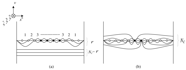
The $s$-rule (3.40) shows that the total number of $M$ theory fivebranes wrapping the vanishing cycles of $Q$ is $r(N_{f}-r)$. These fivebranes (or D fourbranes in Type IIA picture) provide [1] massless hypermultiplets. Actually, for each 2-sphere $C$ we can associate four real parameters: Its position $\vec{w}=(w^{1},w^{2},w^{3})$ in $(x^{7},x^{8},x^{9})$-directions and $w^{4}=i\int_{C}\omega$, where $\omega$ is the Kähler form (3.18). These four parameters provide the vev of one hypermultiplet $q_{\dot{A}}$ by $q_{\dot{1}}=w^{1}+iw^{2}$ and $q_{\dot{2}}=w^{3}+iw^{4}$.

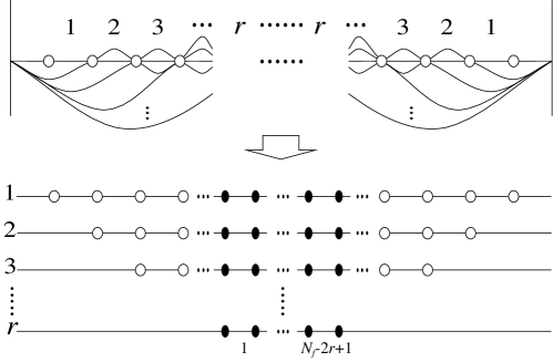
The moduli space ${\cal M}_{\bf nb}^{(r)}$ of the $r$-th non-baryonic branch should be described by these $r(N_{f}-r)$ hypermultiplets. To confirm it let us consider the residual global symmetry of the brane configuration, that is, the symmetry which does not move the brane configuration. We start with a phenomenological argument. Consider the resolution of the degenerated $M$ theory fivebranes or D fourbranes as sketched in Fig.3. There appear $r$ chains of the $M$ theory fivebranes. The $i$-th chain consists of $(N_{f}-2i+1)$ 2-spheres, which give $(N_{f}-2i+1)$ hypermultiplets ${\bf q}_{\dot{A}}^{i}=(q_{\dot{A}}^{i1},\cdots,q_{\dot{A}}^{iN_{f}-2i+1})$. $1\leq i\leq r$. We shall pay attention to the $r$-th chain first. By using $SU(2)_{R}$ and a subgroup $U(N_{f}-2r+1)$ of the flavor group $U(N_{f})$, one may rotate these $(N_{f}-2r+1)$ hypermultiplets ${\bf q}_{\dot{A}}^{r}$ into a normal form, ${\bf q}_{\dot{1}}^{r}=0$ and ${\bf q}_{\dot{2}}^{r}=(d_{r},0,\cdots,0)$ where $d_{r}\in{\bf R}_{>0}$. Then we can see that the residual symmetry of the $r$-th chain is $U(N_{f}-2r)\times U(1)$. The appearance of the extra $U(1)$ symmetry will be shown in the next paragraph. Secondly, we consider the $(r-1)$-th chain. It provides $(N_{f}-2r+3)$ hypermultiplets ${\bf q}_{\dot{A}}^{r-1}=(q_{\dot{A}}^{r-11},\cdots,q_{\dot{A}}^{r-1N_{f}-2r+3})$. One may also rotate these hypermultiplets ${\bf q}_{\dot{A}}^{r-1}$, by using $SU(2)_{R}$ and a subgroup $U(N_{f}-2r+3)$ of $U(N_{f})$, into a normal form, ${\bf q}_{\dot{1}}^{r-1}=0$ and ${\bf q}_{\dot{2}}^{r-1}=(d_{r-1},0,\cdots,0)$. One may expect that the residual symmetry of the $(r-1)$-th chain is $U(N_{f}-2r+2)\times U(1)$. But, looking at Fig.3, it is very plausible that the non-Abelian part $U(N_{f}-2r+2)$ includes $U(N_{f}-2r)$ of the stabilizer of the $r$-th chain. Therefore we must take $U(N_{f}-2r)\times U(1)$ as the residual symmetry of the $(r-1)$-th chain. Repeating the same argument to the 1st chain we obtain $U(N_{f}-2r)\times U(1)^{r}$ as the residual symmetry of the brane configuration. This coincides with the stabilizer of the $r$-th non-baryonic branch described in Section 2.

Figure 3: Resolution of degenerated D fourbranes.

The above phenomenological argument will be justified by using an algebraic description of ${\cal M}_{\bf nb}^{(r)}$. Since we introduce ${\cal M}_{\bf nb}^{(r)}$ as the stratum of ${\cal M}_{\bf nb}$ specified by the symmetry breaking pattern, $SU(N_{c})\rightarrow SU(N_{c}-r)$, or equivalently the condition, ${\rm rank}\,Q_{\dot{A}}=r$ ($c.f.$ (2.26)), we may handle ${\cal M}_{\bf nb}^{(r)}$ by the following regularized complex symplectic quotient for $r\times N_{f}$ complex matrices $H_{\dot{A}}^{(r)}$

$${\cal M}_{\bf nb}^{(r)alg}\equiv\frac{\mu_{\bf C}^{(r)-1}(0)^{s}}{GL(r,{\bf C})},$$ (3.41)

where

$$\mu_{\bf C}^{(r)-1}(0)^{s}=\left\{H^{(r)}_{\dot{A}}\left|\begin{array}[]{l}\cdot~{}\mu_{\bf C}^{(r)}\equiv H^{(r)}_{\dot{1}}H^{(r)\dagger}_{\dot{2}}=0\\ \cdot~{}{\rm rank}\,H^{(r)}_{\dot{1}}=r\end{array}\right.\right\},$$ (3.42)

and $GL(r,{\bf C})$ acts on $H_{\dot{A}}^{(r)}$ by $(H^{(r)}_{\dot{1}},H_{\dot{2}}^{(r)\dagger})$ $\mapsto$ $(gH^{(r)}_{\dot{1}},H_{\dot{2}}^{(r)\dagger}g^{-1})$ where $g\in GL(r,{\bf C})$. A simple parametrization of ${\cal M}_{\bf nb}^{(r)alg}$ is given by

$$H^{(r)}_{\dot{1}} = \left(\begin{array}[]{cc}\phantom{-h^{(r)}_{\dot{2}}h_{\dot{1}}^{(r)\dagger}}&\\ {\bf 1}_{r}&h^{(r)}_{\dot{1}}\\ &\end{array}\right),$$ (3.46)

$$H^{(r)}_{\dot{2}} = \left(\begin{array}[]{cc}&\\ -h^{(r)}_{\dot{2}}h_{\dot{1}}^{(r)\dagger}&h^{(r)}_{\dot{2}}\\ &\end{array}\right),$$ (3.50)

where $h^{(r)}_{\dot{A}}$ are arbitrary $r\times(N_{f}-r)$ complex matrices and will provide the holomorphic coordinates of ${\cal M}^{(r)}_{\rm nb}$. The flavor group $U(N_{f})$, acting on $H^{(r)}_{\dot{A}}$ by $H^{(r)}_{\dot{A}}\mapsto H^{(r)}_{\dot{A}}f$ ($f\in U(N_{f})$), now transforms $h^{(r)}_{\dot{A}}$ as follows :

$$h^{(r)}_{\dot{1}}\mapsto h^{(r)f}_{\dot{1}} = (A+h^{(r)}_{\dot{1}}C)^{-1}(B+h^{(r)}_{\dot{1}}D),$$

$$h^{(r)}_{\dot{2}}\mapsto h^{(r)f}_{\dot{2}} = (A+h^{(r)}_{\dot{1}}C)^{-1}h^{(r)}_{\dot{2}}(-h^{(r)\dagger}_{\dot{1}}B+D),$$ (3.51)

where $f=\left(\begin{array}[]{cc}A&B\\ C&D\end{array}\right)\in U(N_{f})$.

One may construct $r\times(N_{f}-r)$ complex matrices $h^{(r)}_{\dot{A}}$ by arranging the hypermultiplets $q_{\dot{A}}^{ij}$ as follows :

$$h^{(r)}_{\dot{A}}=\left(\begin{array}[]{cccccc}q^{1r}_{\dot{A}}&\cdots&\cdots&\cdots&\cdots&q^{1N_{f}-1}_{\dot{A}}\\ \vdots&q^{2r-1}_{\dot{A}}&\cdots&\cdots&\cdots&q^{2N_{f}-3}_{\dot{A}}\\ \vdots&\vdots&\ddots&&&\vdots\\ q^{11}_{\dot{A}}&q^{21}_{\dot{A}}&\cdots&q^{r1}_{\dot{A}}&\cdots&q_{\dot{A}}^{rN_{f}-2r+1}\end{array}\right).$$ (3.52)

In particular the normal form given in the above phenomenological argument corresponds to

$$h^{(r)}_{\dot{1}} = 0,$$

$$h^{(r)}_{\dot{2}} = \left(\begin{array}[]{ccccccc}d_{1}&&&&&&\\ &d_{2}&&&&&\\ &&\ddots&&&&\\ &&&d_{r}&&&\end{array}\right).$$ (3.57)

By considering $U(N_{f})$-action (3.51) on this form we can also find that the stabilizer is nothing but $U(N_{f}-2r)\times U(1)^{r}$.

3.4 The Baryonic Branch

The $M$ theory realization of the moduli space of the baryonic branch is similar to the description of the non-baryonic branch with $r=N_{f}-N_{c}$ except that the remaining $2N_{c}-N_{f}$ D fourbranes (or a part of the original $M$ theory fivebrane) must be attached to the D sixbranes. This is because the colour symmetry is completely broken at the baryonic branch. The corresponding brane configuration is given in Fig.2(b). In this figure $2N_{c}-N_{f}$ D sixbranes to which these extra D fourbranes are attached are depicted as black circles. $N_{c}(N_{f}-N_{c})$ hypermultiplets given by the $M$ theory fivebranes wrapping the vanishing cycles of $Q$ will parametrize the hyper-Kähler quotient $\widehat{\cal M}_{\bf b}(\zeta_{\dot{A}\dot{B}})$ (2.11) through its algebraic description (2.34). As we noted in Section 2.1, this moduli space gives a resolution of $\cup_{r=0}^{N_{f}-N_{c}}{\cal M}_{\bf nb}^{(r)}$. By comparing the brane configurations of the non-baryonic and baryonic branches one can observe that the extra $2N_{c}-N_{f}$ D fourbranes resolve the non-baryonic branch by suspending the D sixbranes (the black circles in Fig.2(b)).

Two NS fivebranes can now move in $(x^{7},x^{8},x^{9})$-directions since all the D fourbranes are separated by the D sixbranes. Their relative position in $(x^{7},x^{8},x^{9})$-directions, possibly accompanied by their relative position in $x^{10}$-direction, will also provide a hypermultiplet. So, adding this hypermultiplet, we obtain the moduli space ${\cal M}_{\bf b}$ of the baryonic branch.

4 Higgs Branch Root and Duality

In this section we shall examine, from the $M$ theory viewpoint, the root of baryonic branch, where the baryonic branch and the Coulomb branch come in contact with each other. It is discussed in [2] from the field theory viewpoint that the baryonic branch root is a point where the gauge symmetry is quantum mechanically enhanced to $SU(N_{f}-N_{c})\times U(1)^{2N_{c}-N_{f}}$ and the underlying field theory is invariant under the ${\bf Z}_{2N_{c}-N_{f}}$ discrete symmetry (anomaly-free subgroup of $U(1)_{R}$). It is also pointed out that the baryonic branch root admits to have two descriptions which are dual to each other. The “electric” description can be applied if one approaches to the root from the baryonic branch side while the “magnetic” description can be used when one goes to the root from the Coulomb branch side. Our purpose is to understand the duality between these two descriptions in terms of an exchange of NS fivebranes.

The exchange of the NS fivebranes in AF theory or IR-free theory seems difficult to describe. This is because NS fivebranes do not have their definite positions in these theories. (See Fig.1(a) and (b).) To avoid this difficulty it might be convenient to embed these theories into a finite one. (See Fig.1(c).) The Seiberg-Witten curve of $N_{f}=2N_{c}$ finite theory has the form [2, 16]

$$y^{2}-2\prod_{a=1}^{N_{c}}(v-\phi_{a})y+\lambda_{+}\lambda_{-}\prod_{j=1}^{2N_{c}}(v+\lambda_{+}e_{S}-e_{j})=0,$$ (4.1)

where $e_{S}=\frac{1}{2N_{c}}\sum e_{j}$ is the center of the bare masses $e_{j}$ and $\lambda_{\pm}$ are given by

$$\lambda_{+}=-\frac{2F(\tau)}{1-2F(\tau)}~{}~{},~{}~{}~{}\lambda_{-}=-\lambda_{+}+2.$$ (4.2)

Notice that $F(\tau)$ is the following automorphic function of the bare coupling constant $\tau=\frac{\theta}{\pi}+\frac{8\pi i}{g^{2}}$

$$F(\tau)=16q\prod_{n=1}^{\infty}\left(\frac{1+q^{2n}}{1+q^{2n-1}}\right)^{8}$$ (4.3)

with $q=e^{\pi i\tau}$. The modular transforms of $F(\tau)$ are [19]

$$F(\tau)\stackrel{{\scriptstyle T}}{{\mapsto}}F(\tau+1)=\frac{F(\tau)}{F(\tau)-1},{}~{}~{}~{}~{}~{}F(\tau)\stackrel{{\scriptstyle S}}{{\mapsto}}F(-1/\tau)=1-F(\tau),$$ (4.4)

from which we can see that $F(\tau)$ is invariant under the action of the congruence subgroup of level 2, $\Gamma(2)=$ $\left\{\left(\left.\begin{array}[]{cc}a&b\\ c&d\end{array}\right)\in SL(2,{\bf Z})~{}\right|~{}b,c~{}~{}\mbox{even}\right\}$. The Seiberg-Witten curve (4.1) itself admits to have a larger symmetry than $\Gamma(2)$. It is invariant under the following $T^{2}$ and $S$ transforms

$$(\lambda_{\pm}(\tau),~{}e_{j},~{}\phi_{a}) \stackrel{{\scriptstyle T^{2}}}{{\mapsto}} (\lambda_{\pm}(\tau+2)=\lambda_{\pm}(\tau),~{}e_{j},~{}\phi_{a}),$$

$$(\lambda_{\pm}(\tau),~{}e_{j},~{}\phi_{a}) \stackrel{{\scriptstyle S}}{{\mapsto}} (\lambda_{\pm}(-1/\tau)=\lambda_{\mp}(\tau),~{}e_{j}-2e_{s},~{}\phi_{a}).$$ (4.5)

The $M$ theory description of the finite theory tells that the asymptotic positions of the two NS fivebranes in $(x^{6},x^{10})$-directions are given by $\ln\lambda_{\pm}$. In particular their positions in $x^{6}$-direction are $\ln|\lambda_{\pm}|$. Due to the modular property of $F$ the $S$-transform exchanges their asymptotic positions, $\lambda_{\pm}(-1/\tau)=\lambda_{\mp}(\tau)$.

Now let us consider the $Z_{2N_{c}-N_{f}}$ symmetric family of the finite theory :

$$y^{2}-2v^{N_{f}-N_{c}}(v^{2N_{c}-N_{f}}-\varphi^{2N_{c}-N_{f}})y+\lambda_{+}(\tau)\lambda_{-}(\tau)v^{N_{f}}(v^{2N_{c}-N_{f}}-M^{2N_{c}-N_{f}}(\tau))=0,$$ (4.6)

where $\varphi$ is a constant. And we introduce $M^{2N_{c}-N_{f}}(\tau)$ by the following $S$-invariant function

$$M^{2N_{c}-N_{f}}(\tau)=\frac{\Lambda^{2N_{c}-N_{f}}}{F(\tau)(1-F(\tau))},$$ (4.7)

where $\Lambda$ is a constant. The $Z_{2N_{c}-N_{f}}$ symmetry is realized in such a way that curve (4.6) is invariant under the transform, $(v,y)\mapsto(\omega v,\omega^{N_{c}}y)$ where $\omega^{2N_{c}-N_{f}}=1$.

Since $F(\infty)=0$, eq. (4.7) can be regarded as defining a double scaling at the weak coupling limit $\tau\rightarrow i\infty$. In the region $|v|\ll|M|$ the finite curve (4.6) behaves as

$$y^{2}-2v^{N_{f}-N_{c}}(v^{2N_{c}-N_{f}}-\varphi^{2N_{c}-N_{f}})y+4\Lambda^{2N_{c}-N_{f}}v^{N_{f}}=0,$$ (4.8)

which describes the AF theory with colour $SU(N_{c})$ and $N_{f}$ flavor. $\Lambda$ is now the strong-coupling scale of this AF theory. One can approach to the baryonic branch root by tuning $\varphi$ so that $\varphi^{2N_{c}-N_{f}}=-\Lambda^{2N_{c}-N_{f}}$. At this value of $\varphi$ the discriminant of the above AF theory curve becomes a perfect square, which signals an appearance of $2N_{c}-N_{f}$ extra massless hypermultiplets. This is the “electric” description of the baryonic branch root. The baryonic branch of this AF theory is realized in the region $|v|\ll|M|$ of the brane configuration of finite theory (4.6). In this scale, being unable to detect the extra $2N_{c}-N_{f}$ D sixbranes at $v=\omega^{i}M$ $(1\leq i\leq 2N_{c}-N_{f})$, the baryonic branch is given by Fig.2(b) though it is embedded in the finite theory.

What is the brane configuration of the $Z_{2N_{c}-N_{f}}$ symmetric family (4.6) at the strong-coupling regime? We begin by examining how two NS fivebranes behave as the bare coupling constant $g^{2}$ becomes larger. Fix $\theta=0$ for simplicity. Notice that $F(\tau=\frac{8\pi i}{g^{2}})$ is real and monotonically increasing with respect to $g^{2}$. In particular $F$ takes $0,1/2$ respectively at $g^{2}=0,8\pi$. Therefore the relative distance of the two NS fivebranes in $x^{6}$-direction is decreasing as $g^{2}$ becomes larger and it satisfies:

$$\Delta x^{6}=\ln|\lambda_{+}/\lambda_{-}|\rightarrow 0~{}~{}~{}~{}~{}(g^{2}\rightarrow 8\pi).$$ (4.9)

At $g^{2}=8\pi$ (i.e. $\tau=i$) these two NS fivebranes are overlapped in $(v,b)$-plane. In fact, if one rescales $y$ to $\tilde{y}=(1-2F)y$, curve (4.6) acquires the form

$$\tilde{y}^{2}-2(1-2F)v^{N_{f}-N_{c}}(v^{2N_{c}-N_{f}}-\varphi^{2N_{c}-N_{f}})\tilde{y}-4F(1-F)v^{N_{f}}(v^{2N_{c}-N_{f}}-M^{2N_{c}-N_{f}})=0,$$ (4.10)

which shows that $N_{c}$ D fourbranes becomes irrelevant at $g^{2}=8\pi$.

One may expect that the above overlapping of two NS fivebranes is evaded by taking some other route in the upper half plane where the bare coupling constant $\tau$ lives. But it is in vain. Consider a semi-circle $L=\{\tau=ie^{i\alpha}~{}(-\pi/2\leq\alpha\leq\pi/2)\}$ in the upper half plane. Since $F(\tau)$ satisfies the relations $\bar{F}(\tau)=F(-\bar{\tau})$ and $F(-1/\tau)=1-F(\tau)$, it follows that $\mbox{Re}~{}F=1/2$ for ${}^{\forall}\tau\in L$. This means $\ln|\lambda_{+}/\lambda_{-}|=0$ on $L$. Therefore, for any $\tau\in L$, the two NS fivebranes are overlapping in $(v,b)$-plane, at least asymptotically.

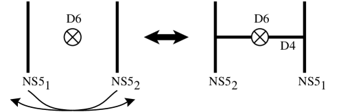
The exchange of the two NS fivebranes will take place on this semi-circle $L$. It is argued in [5] that, when two NS fivebranes are exchanged crossing a D sixbrane, a D fourbrane is created and then suspended between these fivebranes with touching the sixbrane. Conversely, a D fourbrane suspended between these fivebranes with touching the sixbrane is annihilated by this exchange. See Fig.4.

Figure 4: Creation and annihilation of D fourbrane by D sixbrane in Type IIA picture.

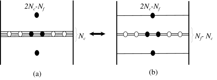
With this process of the exchange the extra $2N_{c}-N_{f}$ D sixbranes located at $v=\omega^{i}M$ $(1\leq i\leq 2N_{c}-N_{f})$ create $2N_{c}-N_{f}$ D fourbranes there, while the $2N_{c}-N_{f}$ D fourbranes touching the D sixbranes at the origin are annihilated. Due to the $s$-rule the brane configuration becomes a “magnetic” configuration depicted in Fig.5. In this “magnetic” configuration (Fig.5(b)) we can find $SU(N_{f}-N_{c})\times U(1)^{2N_{c}-N_{f}}$ SQCD with $N_{f}$ flavor and $2N_{c}-N_{f}$ massless singlet hypermultiplets charged by the $U(1)$ factors, which gives the “magnetic” description [2] of the baryonic branch root. Inside the semi-circle $L$ the electric curve (4.6) will jump to the magnetic one:

$$y^{2}-2v^{N_{f}-N_{c}}(v^{2N_{c}-N_{f}}-M(\tau)^{2N_{c}-N_{f}})y+\lambda_{+}(\tau)\lambda_{-}(\tau)v^{N_{f}}(v^{2N_{c}-N_{f}}-M(\tau)^{2N_{c}-N_{f}})=0.$$ (4.11)

This curve is also invariant under the $S$-transform and one can study it in terms of the dual bare coupling constant $\tilde{\tau}=-1/\tau$.

The $2N_{c}-N_{f}$ massless singlet hypermultiplets obtained from the open string among the extra $2N_{c}-N_{f}$ D sixbranes and the D fourbranes touching them do not have their moduli. Namely they are frozen. The net moduli space of the Higgs branch of this theory is that of $SU(N_{f}-N_{c})$ SQCD with $N_{f}$ flavor. As we have seen in Section 2, the baryonic branch of this IR-free theory is isomorphic to that of $SU(N_{c})$ SQCD with $N_{f}$ flavor.

Figure 5: Brane configurations related by the exchange of the NS fivebranes. (a) is “electric” and (b) is “magnetic”. The case of $(N_{c},N_{f})=(4,6)$ is sketched as an example.

References

- [1] E. Witten, “Solutions of Four-Dimensional Field Theories via M Theory,” hep-th/9703166.
- [2] P. C. Argyres, M. R. Plesser and N. Seiberg, “The Moduli Space of Vacua of N=2 SUSY QCD and Duality in N=1 SUSY QCD,” Nucl. Phys. B471 (1996) 159, hep-th/9603042.
- [3] N. Seiberg, “Electric-Magnetic Duality in Supersymmetric Non-Abelian Gauge Theories,” Nucl. Phys. B435 (1995) 129, hep-th/9411149.
- [4] K. Intriligator and N. Seiberg, “Lectures on Supersymmetric Gauge Theories and Electric-Magnetic Duality,” Nucl. Phys. Proc. Suppl. 45BC (1996) 1, hep-th/9509066
- [5] A. Hanany and E. Witten, “Type IIB Superstrings, BPS Monopoles, and Three-Dimensional Gauge Dynamics,” Nucl. Phys. B492 (1997) 152, hep-th/9611230.
- [6] S. Elitzur, A Giveon and D. Kutasov, “Branes and N=1 Duality in String Theory,” Phys. Lett. B400 (1997) 269, hep-th/9702014
- [7] J. L. F. Barbon, “Rotated Branes and N=1 Duality,” hep-th/9703051
- [8] K. Hori, H. Ooguri and Y.Oz, “Strong Coupling Dynamics of Four-Dimensional N=1 Gauge Theories from M theory Fivebrane,” hep-th/9706082.
- [9] E. Witten, “Branes and The Dynamics of QCD,” hep-th/9706109
- [10] N. Seiberg and E. Witten, “Electric-Magnetic Duality, Monopole Condensation, and Confinement in N=2 Supersymmetric Yang-Mills Theory,” Nucl. Phys. B426 (1994) 19, hep-th/9407087.
- [11] N. Seiberg and E. Witten, “Monopoles, Duality and Chiral Symmetry Breaking in N=2 Supersymmetric QCD,” Nucl. Phys. B431 (1994) 484, hep-th/9408099.
- [12] A. Klemm, W. Lerche, S. Yankielowicz, “Simple Singularities and Supersymmetric Yang-Mills Theory,” Phys. Lett. B344 (1995) 169, hep-th/9411048.
- [13] P. C. Argyres and A. E. Faraggi, “The Vacuum Structure and Spectrum of Supersymmetric Gauge Theory,” Phys. Rev. Lett. 74 (1995) 3931, hep-th/9411057.
- [14] P. K. Townsend, “ The eleven-dimensional supermembrane revisited”, Phys. Lett. B350 (1995) 184, hep-th/9501068.
- [15] A. Hanany and Y. Oz, “On the Quantum Moduli Space of Vacua of Supersymmetric Gauge Theories,” Nucl. Phys. B452 (1995) 283, hep-th/9505075.
- [16] P. C. Argyres, M. R. Plesser and A. D. Shapere, “The Coulomb Phase of N=2 Supersymmetric QCD,” Phys. Rev. Lett. 75 (1995) 1699, hep-th/9505100.
-
[17]
S. W. Hawking, “Gravitational Instantons,” Phys. Lett. 60A (1977) 81.
G. W. Gibbons and S. W. Hawking, “Classification of Gravitational Instanton Symmetries”, Commun. Math. Phys. 66 (1979) 291.
T. Eguchi, B. Gilkey and J. Hansen, Phys. Rep. 66 (1980) 213. - [18] N. J. Hitchin, “Polygons and gravitons,” Math. Proc. Camb. Phil. Soc. 85 (1979) 465.
[19]
L. R. Ford, “Automorphic Functions”, Chelsea Publishing, New York.
E. T. Whittaker and G. W. Watson, “A Course of Modern Analysis”, Cambridge University Press.