Nambu–Jona-Lasinio Model Coupled to Constant
Electromagnetic Fields in $D$-Dimension

Abstract

Critical dynamics of the Nambu–Jona-Lasinio model, coupled to a constant electromagnetic field in $D=2$, $3$, and $4$, is reconsidered from a viewpoint of infrared behavior and vacuum instability. The latter is associated with constant electric fields and cannot be avoidable in the nonperturbative framework obtained through the proper time method. As for magnetic fields, an infrared cut-off is essential to investigate the critical phenomena. The result reconfirms the fact that the critical coupling in $D=3$ and $4$ goes to zero even under an infinitesimal magnetic field. There also shows that a non-vanishing $F_{\mu\nu}\widetilde{F}^{\mu\nu}$ causes instability. A perturbation with respect to external fields is adopted to investigate critical quantities, but the resultant asymptotic expansion excellently matches with the exact value.

I Introduction

The four-fermi interaction model by Nambu and Jona-Lasinio (NJL) [1] has been discussed to investigate the dynamical symmetry breaking (DSB) in a number of cases in two, three, and four dimensions. Especially interesting situations are found such that NJL is coupled to external sources, which enables us to peep into detailed structures of DSB and obtain information on the chiral symmetry breaking ($\chi$SB) in the QCD vacuum, the planar ($2+1$-dimensional) dynamics in solid state physics, or the early universe when coupled to a curved space-time [2]. In this respect the NJL model minimally coupled to the electromagnetic fields is discussed by many authors to explain how $\chi$SB could be changed under the influence of the electromagnetic fields: Klevansky and Lemmer [3] find that a pure electric field opposes $\chi$SB to restore chiral symmetry, meanwhile a pure magnetic field enhances $\chi$SB. The former result has been generalized to non-abelian gauge fields by Suganuma and Tatsumi, where they argue about chiral symmetry restoration by (color) electric fields[4]. Meanwhile the latter result is further investigated by Gusynin, Miransky, and Shovkovy who find that there occurs the mass generation even at the weakest attractive interaction in $2+1$-dimension [5] ($\chi$SB in $2+1$-dimension can be realized as a flavor symmetry breaking by introducing an additional fermion [6]) and in $3+1$-dimension [7] and emphasize it by means of the dimensional reduction. This implies that the critical coupling is zero even if the applying magnetic field is infinitesimal, which might however contradict with a naïve consideration. The motivation for this work lies here.

Our strategy to this issue is: to start with the Euclidean path integral representation of the NJL model minimally coupled to constant electromagnetic fields. Following the standard procedure, that is, introducing auxiliary fields and integrating with respect to the fermion field, we arrive at the pure bosonic path integral consisting of the auxiliary fields and a functional determinant. We then rely on the semi-classical approximation and employ the Fock-Schwinger proper time method [8] in order to define a functional determinant. Although the proper time method can automatically provide a gauge-invariant ultraviolet (UV) regularization in terms of the gamma or zeta function similar to the dimensional regularization, we introduce a cut-off $\Lambda^{2}$ to grasp physical situations better, which, however, still be gauge invariant as well as Lorentz covariant. Moreover an infrared (IR) cut-off $\epsilon$ must also be introduced, since infrared divergences arise when external fields are coupled to a massless state. So far a very little care has been devoted to this fact but it is inevitable in order to discuss effects of electromagnetic fields to the NJL model; since we are interested in the transition from massless to massive states or vice versa under an influence of external fields. From these procedures we obtain the effective potential.

Another issue comes up when an electric field comes into play. The effective potential becomes complex, whose imaginary part implies the vacuum instability because of the creation of fermion and antifermion pairs. (The phenomenon is closely related to the Klein paradox in the one body Dirac equation [9].) However if we notice that the imaginary part behaves as ${\mathrm{e}}^{-m^{2}/E}$ with $E$ being the magnitude of electric field, it is negligible when

$$E<m^{2}\ ,$$ (1)

which leads us to the situation that the magnitude of electric fields must always be infinitesimal. However it is enough to live in this world, since we are interested in a change of a vacuum given by the NJL model to that with external fields, so that we can consider them so small as perturbations. With these spirits, we find that there is no notion of criticality in the pure electric field case, since that is defined through a transition from a massive to a massless state but there is not any state with a mass less than a magnitude of the electric field owing to (1). On the contrary, in a pure magnetic field case, we find critical couplings. They are nonvanishing as far as the infrared cut-off $\epsilon$ is kept finite but eventually become zero when $\epsilon\rightarrow 0$. This reconfirms the results of Gusynin, Miransky, and Shovkovy who have relied on the argument in terms of the dimensional reduction. These results are obtained through perturbations with respect to external fields but a resultant asymptotic expansion is found well matched with the exact value even if the first few terms are adopted. This observation would be interesting.

The paper is organized as follows: in Sec. II, we develop a general formalism for computing an effective potential under constant electromagnetic fields. In the subsequent Sec. III, IV, and V, a pure electric, magnetic, and a non-vanishing $F_{\mu\nu}\widetilde{F}^{\mu\nu}$ ($\equiv\epsilon^{\mu\nu\rho\sigma}F_{\mu\nu}F_{\rho\sigma}/2$) in $D=4$ cases are discussed in order. The final Sec. VI is devoted to conclusion. In Appendix A, calculations of the trace and the determinant in deriving the effective potential are given.

II General Formulation

In this section we describe the model and develop a general formulation for obtaining the one-loop effective potential of the $D$-dimensional NJL model. The Lagrangian for the NJL model minimally coupled to external electromagnetic fields is

$${\cal L}=-\overline{\psi}\Bigl{\{}\gamma_{\mu}\bigl{(}\partial_{\mu}-iA_{\mu}\bigr{)}\Bigr{\}}\psi+{g^{2}\over 2}\left\{\begin{array}[]{ll}\left[\bigl{(}\overline{\psi}\psi\bigr{)}^{2}+\bigl{(}\overline{\psi}i\gamma_{5}\psi\bigr{)}^{2}\right]\ ,&D=2,4\ ,\\ \vspace{1ex}\cr\left[\bigl{(}\overline{\psi}\psi\bigr{)}^{2}+\bigl{(}\overline{\psi}i\gamma_{4}\psi\bigr{)}^{2}+\bigl{(}\overline{\psi}i\gamma_{5}\psi\bigr{)}^{2}\right]\ ,&D=3\ ,\end{array}\right.$$ (2)

where the electromagnetic coupling constant has been absorbed into the definition of $A_{\mu}$. Apart from a usual $4$-dimensional case, $\psi$ is a two-component spinor with gamma matrices

$$\gamma_{\mu}=\sigma_{\mu}\,,\quad\gamma_{5}=-i\gamma_{1}\gamma_{2}\,,\quad\sigma_{\mu\nu}\equiv[\gamma_{\mu},\gamma_{\nu}]/2i=\epsilon_{\mu\nu}\sigma_{3}\,;\quad\mu=1,2\,,$$ (3)

in $2$-dimension. For the $3$-dimensional case, a spinorial representation of the Lorentz group is given by two-component spinors, so that corresponding gamma matrices are $2\times 2$. There is no chiral symmetry. In order to be able to discuss chiral symmetry, we introduce another flavor such that [6]

$$\psi=\left(\begin{array}[]{c}\psi_{1}\\ \psi_{2}\end{array}\right)\ ,\quad\overline{\psi}\equiv\left(\begin{array}[]{cc}\overline{\psi}_{1}&\overline{\psi}_{2}\end{array}\right)\equiv\left(\begin{array}[]{cc}\psi_{1}^{{\dagger}}\sigma_{3}&\psi_{2}^{{\dagger}}\sigma_{3}\end{array}\right)\ ,$$ (4)

and $4\times 4$ gamma matrices

$$\gamma_{\mu}=\left(\begin{array}[]{cc}\sigma_{\mu}&0\\ 0&-\sigma_{\mu}\end{array}\right)\,;\mu=1\sim 3\,,\quad\gamma_{4}=\left(\begin{array}[]{cc}0&{\mathchoice{{\hbox{\boldmath$\displaystyle 1$}}}{{\hbox{\boldmath$\textstyle 1$}}}{{\hbox{\boldmath$\scriptstyle 1$}}}{{\hbox{\boldmath$\scriptscriptstyle 1$}}}}\\ {\mathchoice{{\hbox{\boldmath$\displaystyle 1$}}}{{\hbox{\boldmath$\textstyle 1$}}}{{\hbox{\boldmath$\scriptstyle 1$}}}{{\hbox{\boldmath$\scriptscriptstyle 1$}}}}&0\end{array}\right)\,,\quad\gamma_{5}=\gamma_{1}\gamma_{2}\gamma_{3}\gamma_{4}=\left(\begin{array}[]{cc}0&i{\mathchoice{{\hbox{\boldmath$\displaystyle 1$}}}{{\hbox{\boldmath$\textstyle 1$}}}{{\hbox{\boldmath$\scriptstyle 1$}}}{{\hbox{\boldmath$\scriptscriptstyle 1$}}}}\\ -i{\mathchoice{{\hbox{\boldmath$\displaystyle 1$}}}{{\hbox{\boldmath$\textstyle 1$}}}{{\hbox{\boldmath$\scriptstyle 1$}}}{{\hbox{\boldmath$\scriptscriptstyle 1$}}}}&0\end{array}\right)\ .$$ (5)

The chiral symmetry realizes as

$$\psi\longrightarrow{\rm e}^{i\alpha\gamma_{4}}\psi\,,\quad\psi\longrightarrow{\rm e}^{i\beta\gamma_{5}}\psi\ ,$$ (6)

yielding a global $U(2)$ symmetry which is broken by a mass term into $U(1)\times U(1)$.

The partition function of the model is read as

$$Z[A]\equiv\int\!\!{\mathcal{D}}\psi{\mathcal{D}}\overline{\psi}\exp\left[\!\int\!\!d^{D}x\,{\cal L}\right]$$ (7)

$$= \int\!\!{\mathcal{D}}\sigma{\mathcal{D}}{\mathchoice{{\hbox{\boldmath$\displaystyle\pi$}}}{{\hbox{\boldmath$\textstyle\pi$}}}{{\hbox{\boldmath$\scriptstyle\pi$}}}{{\hbox{\boldmath$\scriptscriptstyle\pi$}}}}{\mathcal{D}}\psi{\mathcal{D}}\overline{\psi}\exp\left[-\!\int\!\!d^{D}x\Bigl{[}{1\over 2g^{2}}\bigl{(}\sigma^{2}+{\mathchoice{{\hbox{\boldmath$\displaystyle\pi$}}}{{\hbox{\boldmath$\textstyle\pi$}}}{{\hbox{\boldmath$\scriptstyle\pi$}}}{{\hbox{\boldmath$\scriptscriptstyle\pi$}}}}^{2}\bigr{)}+\overline{\psi}\Bigl{\{}\gamma_{\mu}\bigl{(}\partial_{\mu}-iA_{\mu}\bigr{)}+\bigl{(}\sigma+i{\mathchoice{{\hbox{\boldmath$\displaystyle\pi\cdot{\mit\Gamma}$}}}{{\hbox{\boldmath$\textstyle\pi\cdot{\mit\Gamma}$}}}{{\hbox{\boldmath$\scriptstyle\pi\cdot{\mit\Gamma}$}}}{{\hbox{\boldmath$\scriptscriptstyle\pi\cdot{\mit\Gamma}$}}}}\bigr{)}\Bigr{\}}\psi\Bigr{]}\right]\ ,$$ (9)

where auxiliary fields, $\sigma$ and $\textstyle\pi$, have been introduced as usual;

$${\mathchoice{{\hbox{\boldmath$\displaystyle\pi\cdot{\mit\Gamma}$}}}{{\hbox{\boldmath$\textstyle\pi\cdot{\mit\Gamma}$}}}{{\hbox{\boldmath$\scriptstyle\pi\cdot{\mit\Gamma}$}}}{{\hbox{\boldmath$\scriptscriptstyle\pi\cdot{\mit\Gamma}$}}}}=\left\{\begin{array}[]{ll}\pi\gamma_{5}&\mbox{for }D=2,4\,,\\ \pi_{1}\gamma_{4}+\pi_{2}\gamma_{5}&\mbox{for }D=3\ .\end{array}\right.$$ (10)

The fermionic integration gives the functional determinant:

$$\int\!\!{\mathcal{D}}\psi{\mathcal{D}}\overline{\psi}\exp\left[-\int\!\!d^{D}x\,\overline{\psi}\Bigl{\{}\gamma_{\mu}\bigl{(}\partial_{\mu}-iA_{\mu}\bigr{)}+\bigl{(}\sigma+i{\mathchoice{{\hbox{\boldmath$\displaystyle\pi\cdot{\mit\Gamma}$}}}{{\hbox{\boldmath$\textstyle\pi\cdot{\mit\Gamma}$}}}{{\hbox{\boldmath$\scriptstyle\pi\cdot{\mit\Gamma}$}}}{{\hbox{\boldmath$\scriptscriptstyle\pi\cdot{\mit\Gamma}$}}}}\bigr{)}\Bigr{\}}\psi\right]$$ (12)

$$\hskip 150.00023pt\equiv{\mathrm{Det}}\Bigl{[}\gamma_{\mu}\bigl{(}\partial_{\mu}-iA_{\mu}\bigr{)}+\bigl{(}\sigma+i{\mathchoice{{\hbox{\boldmath$\displaystyle\pi\cdot{\mit\Gamma}$}}}{{\hbox{\boldmath$\textstyle\pi\cdot{\mit\Gamma}$}}}{{\hbox{\boldmath$\scriptstyle\pi\cdot{\mit\Gamma}$}}}{{\hbox{\boldmath$\scriptscriptstyle\pi\cdot{\mit\Gamma}$}}}}\bigr{)}\Bigr{]}\ .$$

We then perform the semiclassical approximation, that is, shift, $\sigma\rightarrow m+\sigma^{\prime}$, ${\mathchoice{{\hbox{\boldmath$\displaystyle\pi$}}}{{\hbox{\boldmath$\textstyle\pi$}}}{{\hbox{\boldmath$\scriptstyle\pi$}}}{{\hbox{\boldmath$\scriptscriptstyle\pi$}}}}\rightarrow{\mathchoice{{\hbox{\boldmath$\displaystyle\pi$}}}{{\hbox{\boldmath$\textstyle\pi$}}}{{\hbox{\boldmath$\scriptstyle\pi$}}}{{\hbox{\boldmath$\scriptscriptstyle\pi$}}}}^{\prime}$, and assign $\sigma^{\prime}$ and ${\mathchoice{{\hbox{\boldmath$\displaystyle\pi$}}}{{\hbox{\boldmath$\textstyle\pi$}}}{{\hbox{\boldmath$\scriptstyle\pi$}}}{{\hbox{\boldmath$\scriptscriptstyle\pi$}}}}^{\prime}$ as the new integration variables to find

$$Z[A]=\exp\left[-VT{\mbox{$v$}}_{D}(m)\right]\Bigl{(}1+O(\mbox{$2$-loop})\Bigr{)}\ ,$$ (13)

with

$$\mbox{$v$}_{D}(m)\equiv{m^{2}\over 2g^{2}}-{1\over VT}\ln{\mathrm{Det}}\Bigl{[}\gamma_{\mu}\bigl{(}\partial_{\mu}-iA_{\mu}\bigr{)}+m\Bigr{]}\ ,$$ (14)

where $V$ is the $(D-1)$-dimensional volume of the system and $T$ is the Euclidean time interval. (This semiclassical approximation would be more justified by introducing $N$ fermion pieces and taking $N\rightarrow\infty$.) It should be understood that the terms of $O(\mbox{2-loop})$ are given by integrations with respect to $\sigma^{\prime}$ and ${\mathchoice{{\hbox{\boldmath$\displaystyle\pi$}}}{{\hbox{\boldmath$\textstyle\pi$}}}{{\hbox{\boldmath$\scriptstyle\pi$}}}{{\hbox{\boldmath$\scriptscriptstyle\pi$}}}}^{\prime}$. ${\mbox{$v$}}_{D}(m)$ in (14) is the one-loop effective potential from which we can see the phase structure of the model.

In order to make (12) well defined, we normalize it as follows:

$$I_{D} \equiv \ln\left[{{\mathrm{Det}}[\gamma_{\mu}(\partial_{\mu}-iA_{\mu})+m]\over{\mathrm{Det}}[\gamma_{\mu}\partial_{\mu}]}\right]$$ (15)

$$= {\mathrm{Tr}}{\mathrm{Ln}}\Bigl{(}\gamma_{\mu}\bigl{(}\partial_{\mu}-iA_{\mu}\bigr{)}+m\Bigr{)}-{\mathrm{Tr}}{\mathrm{Ln}}\Bigl{(}\gamma_{\mu}\partial_{\mu}\Bigr{)}$$ (16)

$$= {1\over 2}{\mathrm{Tr}}{\mathrm{Ln}}\Bigl{(}-\bigl{(}\partial_{\mu}-iA_{\mu}\bigr{)}^{2}-{1\over 2}\sigma_{\mu\nu}F_{\mu\nu}+m^{2}\Bigr{)}-{1\over 2}{\mathrm{Tr}}{\mathrm{Ln}}\Bigl{(}-\partial_{\mu}^{2}\Bigr{)}\ ,$$ (17)

where the trace operation, designated by ${\mathrm{Tr}}$, must be taken with respect to the space-time as well as the gamma matrices, whereas ${\mathrm{tr}}$ implies that only for the gamma matrices. With the use of the identity,

$$\ln H=-\lim_{s\rightarrow 0}\left[\int_{0}^{\infty}\!d\tau\,\tau^{s-1}{\mathrm{e}}^{-\tau H}-\Gamma(s)\right]\ ,$$ (18)

$I_{D}$ can be rewritten as

$$I_{D} = -{1\over 2}\lim_{s\rightarrow 0}\int_{0}^{\infty}\!d\tau\,\tau^{s-1}{\mathrm{Tr}}\left({\mathrm{e}}^{-\tau[-(\partial_{\mu}-iA_{\mu})^{2}-{1\over 2}\sigma_{\mu\nu}F_{\mu\nu}+m^{2}]}-{\mathrm{e}}^{-\tau[-\partial_{\mu}^{2}]}\right)$$ (19)

$$= -{1\over 2}\lim_{s\rightarrow 0}\int_{0}^{\infty}\!d\tau\,\tau^{s-1}\Biggl{[}{\mathrm{e}}^{-\tau m^{2}}{\mathrm{tr}}({\mathrm{e}}^{{\tau\over 2}\sigma_{\mu\nu}F_{\mu\nu}})\int\!\!d^{D}x\langle x|{\mathrm{e}}^{\tau[(\partial_{\mu}-iA_{\mu})^{2}]}|x\rangle$$ (21)

$$-{\mathrm{tr}}{\bf 1}\int\!\!d^{D}x\langle x|{\mathrm{e}}^{\tau\partial_{\mu}^{2}}|x\rangle\Biggr{]}\ ,$$

where, in the second line, $F_{\mu\nu}$ has been assumed to be constant and $\sigma_{\mu\nu}\equiv\bigl{[}\gamma_{\mu},\gamma_{\nu}\bigr{]}/2i$. The kernel $\langle x|{\mathrm{e}}^{\tau[(\partial_{\mu}-iA_{\mu})^{2}]}|x^{\prime}\rangle$ with a constant $F_{\mu\nu}$ can be calculated by means of the proper time method [8] as

$$\langle x|{\mathrm{e}}^{\tau[(\partial_{\mu}-iA_{\mu})^{2}]}|x^{\prime}\rangle = {1\over(4\pi\tau)^{D/2}}\exp\left[i\int_{x^{\prime}}^{x}\!d\xi_{\mu}A_{\mu}(\xi)\right]\left[\det\left({\sin(\tau F)\over\tau F}\right)\right]^{-{1\over 2}}$$ (23)

$$\hskip 30.0pt\times\exp\left[-{1\over 4\tau}(x-x^{\prime})_{\mu}(\tau F\cot\tau F)_{\mu\nu}(x-x^{\prime})_{\nu}\right]\ ,$$

where $F$ denotes a $D\times D$ matrix whose components are $F_{\mu\nu}$. Combining (21) and (23) we obtain

$$I_{D}=-VT\lim_{s\rightarrow 0}{{\mathrm{tr}}{\bf 1}\over 2(4\pi)^{D/2}}\int_{0}^{\infty}\!d\tau\,\tau^{s-{D\over 2}-1}\left\{{\mathrm{e}}^{-\tau m^{2}}G_{D}(\tau F)-1\right\}\ .$$ (24)

where $G_{D}(\tau F)$ reads

$$G_{D}(\tau F) \equiv {{\mathrm{tr}}({\mathrm{e}}^{{\tau\over 2}\sigma_{\mu\nu}{F}_{\mu\nu}})\over{\mathrm{tr}}{\bf 1}}\left[\det\left({\sin(\tau{F})\over\tau{F}}\right)\right]^{-{1\over 2}}$$ (25)

$$= \left\{\begin{array}[]{lcl}\tau{F}_{D}\coth(\tau{F}_{D})&{\mathrm{for}}&D=2,3\ ,\\ \vspace{1ex}\cr\tau^{2}{F}_{+}{F}_{-}\coth(\tau{F}_{+})\coth(\tau{F}_{-})&{\mathrm{for}}&D=4\ ,\end{array}\right.$$ (28)

with

$$\begin{array}[]{lcl}{F}_{2}&=&E\ ,\\ {F}_{3}&=&\sqrt{B^{2}+{\mathchoice{{\hbox{\boldmath$\displaystyle E$}}}{{\hbox{\boldmath$\textstyle E$}}}{{\hbox{\boldmath$\scriptstyle E$}}}{{\hbox{\boldmath$\scriptscriptstyle E$}}}}^{2}}\ ,\\ {F}_{\pm}&=&\left\{|{\mathchoice{{\hbox{\boldmath$\displaystyle B+E$}}}{{\hbox{\boldmath$\textstyle B+E$}}}{{\hbox{\boldmath$\scriptstyle B+E$}}}{{\hbox{\boldmath$\scriptscriptstyle B+E$}}}}|\pm|{\mathchoice{{\hbox{\boldmath$\displaystyle B-E$}}}{{\hbox{\boldmath$\textstyle B-E$}}}{{\hbox{\boldmath$\scriptstyle B-E$}}}{{\hbox{\boldmath$\scriptscriptstyle B-E$}}}}|\right\}/2\ .\end{array}$$ (29)

(Details are shown in Appendix A.) As was mentioned above ${\mathrm{tr}}{\bf 1}$ in (24) and (28) is $2^{D/2}$ for $D=2,4$ and $2^{(D+1)/2}$ for $D=3$. Although the integral (24) has entirely been regularized if an analytic continuation is made for $s$, in order to grasp a physical situation better, an UV cut-off $\Lambda^{2}$ is introduced as is done in the ordinary gap equation [1]. Moreover, an IR cut-off $\epsilon$ is indispensable, since if $m^{2}=0$ and $F\neq 0$, the integral (24) becomes divergent. Therefore we consider instead of (24)

$${I_{D}}^{\mathrm{r}}\equiv-VT{{\mathrm{tr}}{\bf 1}\over 2(4\pi)^{D/2}}\int_{1/\Lambda^{2}}^{\infty}\!d\tau\,\tau^{-{D\over 2}-1}\left\{{\mathrm{e}}^{-\tau(m^{2}+\epsilon)}G_{D}(\tau F)-1\right\}\ .$$ (30)

This regularized ${{I}_{D}}^{\mathrm{r}}$ enables us to investigate dynamics near the massless region, so does that of $\chi$SB. Now the well-defined effective potential is given by

$${\mbox{$v$}}_{D}(m)={m^{2}\over 2g^{2}}+{{\mathrm{tr}}{\bf 1}\over 2(4\pi)^{D/2}}\int_{1/\Lambda^{2}}^{\infty}\!d\tau\,\tau^{-{D\over 2}-1}\left\{{\mathrm{e}}^{-\tau(m^{2}+\epsilon)}G_{D}(\tau F)-1\right\}\ .$$ (31)

We then introduce dimensionless quantities, $x\equiv(m^{2}+\epsilon)/\Lambda^{2}$ and ${\cal F}\equiv F/\Lambda^{2}$ $({\cal F}_{\mu\nu}\equiv F_{\mu\nu}/\Lambda^{2})$, obeying $\epsilon/\Lambda^{2}\leq x<1$ and $|{\cal F}_{\mu\nu}|<1$. (Recall that mass dimension of the gauge field is always one because of inclusion of the coupling constant.) Therefore the (dimensionless) effective potential $\overline{\mbox{$v$}}_{D}(x)$ is read as

$$\overline{\mbox{$v$}}_{D}(x)\equiv{2(4\pi)^{D/2}\over{\mathrm{tr}}{\bf 1}\,\Lambda^{D}}{\mbox{$v$}}_{D}(m)={(4\pi)^{D/2}\over{\mathrm{tr}}{\bf 1}\,g^{2}\Lambda^{D-2}}\left(x-{\epsilon\over\Lambda^{2}}\right)+\int_{1}^{\infty}\!\!d\tau\,\tau^{-{D\over 2}-1}\left\{{\mathrm{e}}^{-\tau x}G_{D}(\tau{\cal F})-1\right\}\ .$$ (32)

The stationary condition, $\partial{\mbox{$v$}}_{D}(m)/\partial m=0$, is

$${\partial\,\overline{\mbox{$v$}}_{D}(x)\over\partial(m/\Lambda)}={2m\over\Lambda}\left[{(4\pi)^{D/2}\over{\mathrm{tr}}{\bf 1}\,g^{2}\Lambda^{D-2}}+f_{D}(x)\right]=0\ ,$$ (33)

where $f_{D}(x)$ is defined as

$$f_{D}(x)\equiv{\partial\over\partial x}\int_{1}^{\infty}\!\!d\tau\,\tau^{-{D\over 2}-1}{\mathrm{e}}^{-\tau x}G_{D}(\tau{\cal F})\ .$$ (34)

Thus the equation for non-trivial solutions of (33), the gap equation, is

$$-{(4\pi)^{D/2}\over{\mathrm{tr}}{\bf 1}\,g^{2}\Lambda^{D-2}}=f_{D}(x)\ .$$ (35)

Hereafter we designate the stationary point, the solution of the gap equation, as $x^{*}(=({m^{*}}^{2}+\epsilon)/\Lambda^{2})$. The stability condition $\partial^{2}{\mbox{$v$}}_{D}(m)/\partial m^{2}|_{m^{*}}\geq 0$, gives

$${\partial^{2}\,\overline{\mbox{$v$}}_{D}(x)\over\partial(m/\Lambda)^{2}}\Biggr{|}_{x=x^{*}}={4m^{2}\over\Lambda^{2}}f^{\prime}_{D}(x^{*})\geq 0\ ,$$ (36)

where use has been made of (35), and then, the absolute minimum condition, ${\mbox{$v$}}_{D}(m^{*})-{\mbox{$v$}}_{D}(0)\leq 0$, leads to

$$\overline{\mbox{$v$}}_{D}(x^{*})-\overline{\mbox{$v$}}_{D}(\epsilon/\Lambda^{2}) = \int_{\epsilon/\Lambda^{2}}^{x^{*}}\!dx\,f_{D}(x)+{(4\pi)^{D/2}\over{\mathrm{tr}}{\bf 1}\,g^{2}\Lambda^{D-2}}{{m^{*}}^{2}\over\Lambda^{2}}$$ (37)

$$= \int_{\epsilon/\Lambda^{2}}^{x^{*}}dx\,\left[f_{D}(x)-f_{D}(x^{*})\right]\leq 0\ .$$ (38)

Finally, we list the integral expression for the effective potential in each dimension,

$$\overline{\mbox{$v$}}_{2}(x) = {2\pi\over g^{2}}\left(x-{\epsilon\over{\Lambda}^{2}}\right)+\int_{1}^{\infty}\!\!d\tau\,\tau^{-2}{\mathrm{e}}^{-\tau x}(\tau{\cal F}_{2})\coth(\tau{\cal F}_{2})\ ,$$ (39)

$$\overline{\mbox{$v$}}_{3}(x) = {2{\pi}^{3/2}\over g^{2}\Lambda}\left(x-{\epsilon\over{\Lambda}^{2}}\right)+\int_{1}^{\infty}\!\!d\tau\,\tau^{-{5\over 2}}{\mathrm{e}}^{-\tau x}(\tau{\cal F}_{3})\coth(\tau{\cal F}_{3})\ ,$$ (40)

$$\overline{\mbox{$v$}}_{4}(x) = {4{\pi}^{2}\over g^{2}\Lambda^{2}}\left(x-{\epsilon\over{\Lambda}^{2}}\right)+\int_{1}^{\infty}\!\!d\tau\,\tau^{-3}{\mathrm{e}}^{-\tau x}(\tau^{2}{\cal F}_{+}{\cal F}_{-})\coth(\tau{\cal F}_{+})\coth(\tau{\cal F}_{-})\ ,$$ (41)

where we have ignored the terms independent of mass and fields.

III Constant Electric Field

In this section analyses of a constant electric field are made. (The case reads, covariantly in the Minkowski metric, $F_{\mu\nu}F^{\mu\nu}<0$ as well as $F_{\mu\nu}\widetilde{F}^{\mu\nu}=\epsilon_{\mu\nu\lambda\rho}F^{\mu\nu}F^{\lambda\rho}/2=0$ in $4$-dimension.) As was mentioned in the introduction, an imaginary part arises in the effective potential: the integral in (34) becomes

$$\int_{1}^{\infty}\!\!d\tau\,\tau^{-{D\over 2}-1}{\mathrm{e}}^{-\tau x}(\tau{{\cal E}})\coth(\tau{{\cal E}})\quad{\mathrm{for}}\quad D=2,3,4\ ,$$ (42)

where ${\cal E}$ is the magnitude of the electric field in the $\Lambda^{2}$ unit ($0\leq{\cal E}<1$). To see the imaginary part, go back to the Minkowski space via an analytic continuation, ${\cal E}\rightarrow-i{\cal E}$, obtaining

$$\int_{1}^{\infty}\!\!d\tau\,\tau^{-{D\over 2}-1}{\mathrm{e}}^{-\tau x}(\tau{{\cal E}})\coth(\tau{{\cal E}})$$ (43)

$$\longrightarrow {\mathrm{P}}\!\int_{1}^{\infty}\!\!d\tau\,\tau^{-{D\over 2}-1}{\mathrm{e}}^{-\tau x}(\tau{{\cal E}})\cot(\tau{{\cal E}})-i\pi\sum_{n=1}^{\infty}\left({\cal E}\over n\pi\right)^{D/2}{\mathrm{e}}^{-{n\pi\over{\cal E}}x}$$ (44)

with ${\mathrm{P}}$ denoting the principal value. The sum of the imaginary part (identical to the modified zeta function) is rewritten as,

$$\pi\sum_{n=1}^{\infty}\left({\cal E}\over n\pi\right)^{D/2}{\mathrm{e}}^{-{n\pi\over{\cal E}}x}={{\cal E}^{D/2}\over\pi^{D/2-1}\Gamma(D/2)}\int_{0}^{\infty}\!\!dt{t^{D/2-1}\over{\mathrm{e}}^{t+\pi x/{\cal E}}-1}\ .$$ (45)

In $D=2$, the integral can be performed explicitly, to give

$$-{\cal E}\,{\mathrm{ln}}\!\left(1-{\mathrm{e}}^{-{\pi x\over{\cal E}}}\right)\ .$$ (46)

In view of (45) (or (46)), the imaginary part becomes significant when ${\cal E}>x$ ($E>m^{2}$), which is a rather well-known result from a one-body problem of the Dirac particle under an external potential — the Klein paradox. The appearance of the imaginary part implies the vacuum instability by means of external electric fields [9]. The initial vacuum goes to a new one with emissions of particle pairs to neutralize the electric field which, however, has assumed constant so that the process will never end. To avoid the situation electric fields must be localized [4] or the condition,

$${\cal E}<x\ ,$$ (47)

must be assumed. (See Fig. 1.) Moreover if a perturbative expansion in terms of the electric field is employed we cannot see any imaginary part at all since ${\cal E}=0$ is an essential singularity. The program matches with our strategy. As was stated in the introduction, our interest lies in seeking a change when external fields are present, then it is enough to regard external fields to be very small: perturbations would be useful.

Here we should make three comments.

• According to the condition (47) there is no need for an infrared cut-off in this case so that we put $\epsilon=0$ hereafter.

• It is impossible to talk about criticality of electric fields [3], since it is defined through a massless condition under the variation of electric fields, which contradicts the condition (47).

• The calculation is performed in the Euclidean world throughout. (In the above, we visited in the Minkowski space just because of glancing at the infrared structure.)

With these spirits we first expand the integrand in (42) such that

$$t\coth t=1+{t^{2}\over 3}+O(t^{4})$$ (48)

then integrate each term, and perform the analytic continuation ${\cal E}\rightarrow-i{\cal E}$, to obtain
$D=2$ case:

$$\overline{\mbox{$v$}}_{2}(x)={2\pi\over g^{2}}x+xE_{i}(-x)+\left(1-{{\cal E}^{2}\over 3x}\right){\mathrm{e}}^{-x}-1\ ,$$ (49)

$$-{2\pi\over g^{2}}=f_{2}(x)=Ei(-x)+{{\cal E}^{2}\over 3}\left({1\over x}+{1\over x^{2}}\right){\mathrm{e}}^{-x}\ ,$$ (50)

$D=3$ case:

$$\overline{\mbox{$v$}}_{3}(x)={2\pi^{3/2}\over g^{2}\Lambda}x+{1\over 3}\left(4x-{{\cal E}^{2}\over x}\right)x^{1/2}{\mit\Gamma}(1/2,x)+{2\over 3}(1-2x){\mathrm{e}}^{-x}-{2\over 3}\ ,$$ (51)

$$-{2\pi^{3/2}\over g^{2}\Lambda}=f_{3}(x)=\left(2+{{\cal E}^{2}\over 6x^{2}}\right)x^{1/2}{\mit\Gamma}(1/2,x)-\left(2-{{\cal E}^{2}\over 3x}\right){\mathrm{e}}^{-x}\ ,$$ (52)

$D=4$ case:

$$\overline{\mbox{$v$}}_{4}(x)={4\pi^{2}\over g^{2}\Lambda^{2}}x-\left({x^{2}\over 2}-{{\cal E}^{2}\over 3}\right)E_{i}(-x)+{1\over 2}(1-x){\mathrm{e}}^{-x}-{1\over 2}\ ,$$ (53)

$$-{4\pi^{2}\over g^{2}\Lambda^{2}}=f_{4}(x)=-xE_{i}(-x)-\left(1-{{\cal E}^{2}\over 3x}\right){\mathrm{e}}^{-x}\ .$$ (54)

Here use has been made of

$$-E_{i}(-z)=\int_{z}^{\infty}\!\!dt\,{\mathrm{e}}^{-t}t^{-1}=\int_{1}^{\infty}\!\!dt{\mathrm{e}}^{-tz}t^{-1}\ ,$$ (55)

and

$${\mit\Gamma}(1/2,z)=\int_{z}^{\infty}\!\!dt\,{\mathrm{e}}^{-t}t^{-1/2}\ .$$ (56)

As was expected from the above argument there is no imaginary part. It should be noted that our perturbation expansion (48) is of course an asymptotic expansion to the effective potential (39) – (41) since we have regarded $t$ in (48) as $\tau{\cal E}$ which apparently exceeds the radius of convergence when $\tau\rightarrow\infty$.

We plot $f_{D}(x)$ in Fig. 2 (a)–(c) for several fixed values of ${\cal E}$. First note that in each plot, the thin-dashed line denoting $f_{D}(x)|_{{\cal E}=x}$ shows the lower bound of $x$ (47): the vacuum is unstable in the left region to the line. From the figures we can see that the external electric field makes the mass smaller for a given coupling. This can more easily be seen from Fig. 3 (a)–(c) where the relation between ${\cal E}$ and $x$ are depicted for several fixed values of $g^{2}$. In each plot, the thin-dashed line denoting ${\cal E}=x$, again shows the lower bound of $x$ (47); the vacuum is unstable in the upper triangular region. $g_{c}^{2}$ in (b) and (c) are the critical couplings without any external fields in $D=3$ and $4$ and given by $\pi^{3/2}/\Lambda$ and $4\pi^{2}/\Lambda^{2}$ respectively.

Finally it is necessary to discuss plausibility of our approximation. By changing the integration variable such as $\tau x\rightarrow\tau$, (42) is rewritten as

$$x^{{D\over 2}}\int_{x}^{\infty}\!\!d\tau\,\tau^{-{D\over 2}-1}{\mathrm{e}}^{-\tau}({\tau{\cal E}\over x})\coth({\tau{\cal E}\over x})\ .$$ (57)

Therefore our approximation becomes good when

$${x\over{\cal E}}\rightarrow\infty\ .$$ (58)

However, as is seen from Fig. 4, where the integral (42) for $D=4$ with ${\cal E}=0.25$ is depicted as the function of $x$, matching is excellent for any $x$ down to ${\cal E}$.

IV Constant Magnetic Field

The case for a constant magnetic field is considered in this section. (This reads, covariantly in the Minkowski space, $F_{\mu\nu}F^{\mu\nu}>0$ with $F_{\mu\nu}\widetilde{F}^{\mu\nu}=0$ in $4$-dimension.) Contrary to the previous case, there arises no imaginary part in the effective potential: the integral in (34) reads

$$\int_{1}^{\infty}\!\!d\tau\,\tau^{-{D\over 2}-1}{\mathrm{e}}^{-\tau x}\tau{{\cal B}}\coth(\tau{{\cal B}})$$ (59)

with ${\cal B}$ denoting a magnitude of the magnetic field in the $\Lambda^{2}$ unit ($0\leq{\cal B}<1$). There is no need for an analytic continuation so that any imaginary part does not occur. Therefore, unlike the electric case, there is no restriction on ${\cal B}$ and $x$ (except for $0\leq{\cal B}<1$ and $0\leq x<1$) such as (47), which enforce us to keep $\epsilon$ non zero and to modify the naïve expansion (48), since in this case ${\cal B}/x$ can become large contrary to the electric case where ${\cal E}/x<1$ from (47). We thus arrange (59) such that

$$\int_{1}^{\infty}\!\!d\tau\,\tau^{-{D\over 2}-1}{\mathrm{e}}^{-\tau x}(\tau{\cal B})\coth(\tau{\cal B})$$ (60)

$$= {\cal B}\int_{1}^{\infty}\!\!d\tau\,\tau^{-{D\over 2}}{\mathrm{e}}^{-\tau x}+\int_{1}^{\infty}\!\!d\tau\,\tau^{-{D\over 2}-1}{\mathrm{e}}^{-\tau(x+2{\cal B})}{2\tau{\cal B}\over 1-{\mathrm{e}}^{-2\tau{\cal B}}}\ .$$ (61)

The last factor in the second integral can be expanded as

$${t\over{\mathrm{e}}^{t}-1}=1-{t\over 2}+{t^{2}\over 12}+O(t^{4})\ ,$$ (62)

and then all the term can be evaluated with the use of (55) or (56). This gives an improved asymptotic expansion. The results are read as follows:
$D=3$ case:

$$\overline{\mbox{$v$}}_{3}(x) = {2\pi^{3/2}\over g^{2}\Lambda}\left(x-{\epsilon\over\Lambda^{2}}\right)+{1\over 3}\left[2(2x+{\cal B})+{{\cal B}^{2}\over x+2{\cal B}}\right](x+2{\cal B})^{1/2}{\mit\Gamma}(1/2,x+2{\cal B})$$ (64)

$$+{2\over 3}(1-2x-{\cal B}){\mathrm{e}}^{-(x+2{\cal B})}-2{\cal B}\left[x^{1/2}{\mit\Gamma}(1/2,x)-{\mathrm{e}}^{-x}\right]-{2\over 3}\ ,$$

$$-{2\pi^{3/2}\over g^{2}\Lambda}=f_{3}(x) = \left[2-{{\cal B}\over x+2{\cal B}}-{{\cal B}^{2}\over 6(x+2{\cal B})^{2}}\right](x+2{\cal B})^{1/2}{\mit\Gamma}(1/2,x+2{\cal B})$$ (66)

$$-\left[2+{{\cal B}^{2}\over 3(x+2{\cal B})}\right]{\mathrm{e}}^{-(x+2{\cal B})}-{\cal B}x^{-1/2}{\mit\Gamma}(1/2,x)\ .$$

$D=4$ case:

$$\overline{\mbox{$v$}}_{4}(x) = {4\pi^{2}\over g^{2}\Lambda^{2}}\left(x-{\epsilon\over\Lambda^{2}}\right)-\left({x^{2}\over 2}+x{\cal B}+{{\cal B}^{2}\over 3}\right)E_{i}(-(x+2{\cal B}))$$ (68)

$$+{1\over 2}(1-x){\mathrm{e}}^{-(x+2{\cal B})}+{\cal B}\left[xE_{i}(-x)+{\mathrm{e}}^{-x}\right]-{1\over 2}\ ,$$

$$-{4\pi^{2}\over g^{2}\Lambda^{2}}=f_{4}(x)=-(x+{\cal B})E_{i}(-(x+2{\cal B}))-\left(1+{{\cal B}^{2}\over 3(x+2{\cal B})}\right){\mathrm{e}}^{-(x+2{\cal B})}+{\cal B}E_{i}(-x)\ .$$ (69)

We plot $f_{D}(x)$ in Fig. 5 (a) and (b) for several fixed values of ${\cal B}$, from which we see that any point on the line fulfills the condition $f^{\prime}_{D}(x^{*})\geq 0$, (36). The condition (38) is also satisfied, since (38) is always true for any monotonically increasing $f_{D}(x)$. Since the minimum of $x$ is $\epsilon/\Lambda^{2}$, a finite critical coupling exists as a solution of (35) at $x=\epsilon/\Lambda^{2}$;

$$g^{2}_{c}(\epsilon)\equiv-{(4\pi)^{D/2}\over{\mathrm{tr}}{\bf 1}\,\Lambda^{D-2}f_{D}(\epsilon/\Lambda^{2})}$$ (70)

for a fixed ${\cal B}$. However, when $\epsilon/\Lambda^{2}\rightarrow 0$, $f_{D}(\epsilon/\Lambda^{2})$ behaves as

$$f_{3}(\epsilon/\Lambda^{2}) \sim -{\cal B}(\epsilon/\Lambda^{2})^{-1/2}\Gamma(1/2,\epsilon/\Lambda^{2})+O\left((\epsilon/\Lambda^{2})\right)\ ,$$ (71)

$$f_{4}(\epsilon/\Lambda^{2}) \sim {\cal B}E_{i}(-\epsilon/\Lambda^{2})+O\left((\epsilon/\Lambda^{2})\right)\ ,$$ (72)

so that $f_{D}(\epsilon/\Lambda^{2})\rightarrow-\infty$, as far as ${\cal B}\neq 0$. This implies that the critical coupling goes to zero, $g_{c}\rightarrow 0$, for any non-zero ${\cal B}$. The situation is similar to the 2-dimensional case without external fields, where from (50)

$$f_{2}(x)=E_{i}(-x)\ ,$$ (73)

which is again divergent when $x\rightarrow 0$. Keeping IR cut-off $\epsilon$ finite, we obtain a finite critical coupling

$$g_{c}^{2}(\epsilon)=-{2\pi\over f_{2}(\epsilon/\Lambda^{2})}\ ,$$ (74)

which also becomes zero when $\epsilon/\Lambda^{2}\rightarrow 0$. (Compare Fig. 5 (b) with the ${\cal E}=0$ case of Fig. 2 (a).) Gusynin, Miransky, and Shovkovy have interpreted this similarity in terms of the dimensional reduction [7].

We can also see, from Fig. 5 (a) and (b), that the dynamically generated mass in a constant magnetic field is larger than that without any external field for a fixed coupling. This can more easily be seen from Fig. 6 (a) and (b), where the relations between ${\cal B}$ and $x$ is depicted for several fixed values of $g^{2}$.

We adopt the improved expansion (61) with (62) against the previous one (48). The expansion becomes exact when $1+x/(2{\cal B})\rightarrow\infty$, which can be recognized by looking at the second term in the right-hand side of (61). However as is seen from Fig. 7, matching to the exact value is much more excellent than the previous case in Fig. 4, even if only the first three terms are taken into account.

V General Constant Fields in D=4

So far, in D=4, the case $F_{\mu\nu}\tilde{F}^{\mu\nu}=0$ (in the Minkowski metric), that is, ${\mathchoice{{\hbox{\boldmath$\displaystyle B\cdot E$}}}{{\hbox{\boldmath$\textstyle B\cdot E$}}}{{\hbox{\boldmath$\scriptstyle B\cdot E$}}}{{\hbox{\boldmath$\scriptscriptstyle B\cdot E$}}}}=0$ has been assumed, but in this section a more general case $F_{\mu\nu}\tilde{F}^{\mu\nu}\neq 0$, is considered. We vary $F_{\mu\nu}\tilde{F}^{\mu\nu}$ with $F_{\mu\nu}{F}^{\mu\nu}$ being fixed, which is interpreted, for example, such that the angle between $\textstyle B$ and $\textstyle E$ is shifted from $\pi/2$, while keeping the magnitude of $\textstyle B$ and $\textstyle E$ fixed.

In this case, imaginary parts in the effective potential are also unavoidable. To see this, the analytic continuation $|{\mathchoice{{\hbox{\boldmath$\displaystyle E$}}}{{\hbox{\boldmath$\textstyle E$}}}{{\hbox{\boldmath$\scriptstyle E$}}}{{\hbox{\boldmath$\scriptscriptstyle E$}}}}|\rightarrow-i|{\mathchoice{{\hbox{\boldmath$\displaystyle E$}}}{{\hbox{\boldmath$\textstyle E$}}}{{\hbox{\boldmath$\scriptstyle E$}}}{{\hbox{\boldmath$\scriptscriptstyle E$}}}}|$ is performed in the third relation in (29) and a covariant notation is adopted, such that

$$F_{\mu\nu}F^{\mu\nu} = 2({\mathchoice{{\hbox{\boldmath$\displaystyle B$}}}{{\hbox{\boldmath$\textstyle B$}}}{{\hbox{\boldmath$\scriptstyle B$}}}{{\hbox{\boldmath$\scriptscriptstyle B$}}}}^{2}-{\mathchoice{{\hbox{\boldmath$\displaystyle E$}}}{{\hbox{\boldmath$\textstyle E$}}}{{\hbox{\boldmath$\scriptstyle E$}}}{{\hbox{\boldmath$\scriptscriptstyle E$}}}}^{2})\ ,$$ (75)

$$F_{\mu\nu}\widetilde{F}^{\mu\nu} = -4{\mathchoice{{\hbox{\boldmath$\displaystyle B\cdot E$}}}{{\hbox{\boldmath$\textstyle B\cdot E$}}}{{\hbox{\boldmath$\scriptstyle B\cdot E$}}}{{\hbox{\boldmath$\scriptscriptstyle B\cdot E$}}}}\ ,$$ (76)

giving

$${F}_{+}^{E} \rightarrow {1\over 2}\sqrt{\sqrt{(F_{\mu\nu}F^{\mu\nu})^{2}+(F_{\mu\nu}\widetilde{F}^{\mu\nu})^{2}}+F_{\mu\nu}F^{\mu\nu}}\equiv F_{+}\ ,$$ (77)

$${F}_{-}^{E} \rightarrow {i\over 2}{\mathrm{sgn}}(F_{\mu\nu}\widetilde{F}^{\mu\nu})\sqrt{\sqrt{(F_{\mu\nu}F^{\mu\nu})^{2}+(F_{\mu\nu}\widetilde{F}^{\mu\nu})^{2}}-F_{\mu\nu}F^{\mu\nu}}\equiv-i{F}_{-}\ ,$$ (78)

where ${\mathrm{sgn}}(x)$ designates the sign function

$${\mathrm{sgn}}(x)\equiv\left\{\begin{array}[]{rl}1&(x\geq 0)\ ,\\ -1&(x<0)\ ,\end{array}\right.$$ (79)

and the notation $F_{\pm}^{E}$ has been employed to distinguish the Euclidean quantities from the Minkowski ones. Since there exists a suitable Lorentz frame where $|{\mathchoice{{\hbox{\boldmath$\displaystyle B$}}}{{\hbox{\boldmath$\textstyle B$}}}{{\hbox{\boldmath$\scriptstyle B$}}}{{\hbox{\boldmath$\scriptscriptstyle B$}}}}^{\prime}|=F_{+}$, $|{\mathchoice{{\hbox{\boldmath$\displaystyle E$}}}{{\hbox{\boldmath$\textstyle E$}}}{{\hbox{\boldmath$\scriptstyle E$}}}{{\hbox{\boldmath$\scriptscriptstyle E$}}}}^{\prime}|=|F_{-}|$, and ${\mathchoice{{\hbox{\boldmath$\displaystyle B$}}}{{\hbox{\boldmath$\textstyle B$}}}{{\hbox{\boldmath$\scriptstyle B$}}}{{\hbox{\boldmath$\scriptscriptstyle B$}}}}^{\prime}\parallel{\mathchoice{{\hbox{\boldmath$\displaystyle E$}}}{{\hbox{\boldmath$\textstyle E$}}}{{\hbox{\boldmath$\scriptstyle E$}}}{{\hbox{\boldmath$\scriptscriptstyle E$}}}}^{\prime}$, we regard $F_{+}$ ($F_{-}$) as a Lorentz invariant magnetic (electric) field. The integral in (41) becomes, after the analytic continuation, to

$$\int_{1}^{\infty}\!\!d\tau\,\tau^{-3}{\mathrm{e}}^{-\tau x}(\tau^{2}{\cal F}_{+}^{E}{\cal F}_{-}^{E})\coth(\tau{\cal F}_{+}^{E})\coth(\tau{\cal F}_{-}^{E})$$ (80)

$$\longrightarrow {\mathrm{P}}\int_{1}^{\infty}\!\!d\tau\,\tau^{-3}{\mathrm{e}}^{-\tau x}(\tau^{2}{\cal F}_{+}{\cal F}_{-})\coth(\tau{\cal F}_{+})\cot(\tau{\cal F}_{-})$$ (82)

$$\hskip 20.0pt-i\pi\sum_{n=1}^{\infty}\left({\cal{\cal F}_{+}{\cal F}_{-}}\over n\pi\right){\mathrm{e}}^{-{n\pi\over{\cal F}_{-}}x}\coth\left({n\pi{\cal F}_{+}\over{\cal F}_{-}}\right)$$

with ${\cal F}_{+}=F_{+}/\Lambda^{2}$ and ${\cal F}_{-}=|F_{-}|/\Lambda^{2}$, obeying $0\leq{\cal F}_{\pm}<1$. (The sign of $F_{-}$ or $F_{\mu\nu}\widetilde{F}^{\mu\nu}$ is irrelevant because of parity invariance.) From (82), ${\cal F}_{-}$ is solely responsible for the imaginary part as is expected. (When ${\cal F}_{+}\rightarrow 0$ there remains the imaginary part.) Therefore, as was done in the electric field case, we must set the condition

$${\cal F}_{-}<x$$ (83)

for not having a large imaginary part, which enables us to put $\epsilon\rightarrow 0$ and again prevent us from talking about criticality of the coupling and external fields.

Now go back to the Euclidean world and regard ${\cal F}_{+}^{E}$ and ${\cal F}_{-}^{E}$ as perturbations as before. Follow the same procedure as in the preceding section: first expand the integrand in the left-hand side of (82) such that

$$\int_{1}^{\infty}\!\!d\tau\,\tau^{-3}{\mathrm{e}}^{-\tau x}(\tau^{2}{\cal F}_{+}^{E}{\cal F}_{-}^{E})\coth(\tau{\cal F}_{+}^{E})\coth(\tau{\cal F}_{-}^{E})$$ (84)

$$\simeq {\cal F}_{+}^{E}\int_{1}^{\infty}\!\!d\tau\,\tau^{-2}{\mathrm{e}}^{-\tau x}\Big{[}(\tau{\cal F}_{-}^{E})\coth(\tau{\cal F}_{-}^{E})\Big{]}$$ (86)

$$+\int_{1}^{\infty}\!\!d\tau\,\tau^{-3}{\mathrm{e}}^{-\tau(x+2{\cal F}_{+}^{E})}\left[1+\tau{\cal F}_{+}^{E}+{2\over 3}(\tau{\cal F}_{+}^{E})^{2}\right]\Big{[}(\tau{\cal F}_{-}^{E})\coth(\tau{\cal F}_{-}^{E})\Big{]}\ ,$$

where we have employed the relations (61) and (62) developed in the pure magnetic field case, which is an extremely good expansion. Then we expand $(\tau{\cal F}_{-}^{E})\coth(\tau{\cal F}_{-}^{E})$ by using the expansion (48), integrate each term, and make analytic continuation, ${\cal F}_{-}^{E}\rightarrow-i{\cal F}_{-}$, to obtain

$$\overline{\mbox{$v$}}_{4}(x) = {4{\pi}^{2}\over g^{2}\Lambda^{2}}x+{\cal F}_{+}\left[xEi(-x)+\left(1-{{\cal F}_{-}^{2}\over 3x}\right){\mathrm{e}}^{-x}\right]-\left[{x^{2}\over 2}+x{\cal F}_{+}+{{\cal F}_{+}^{2}-{\cal F}_{-}^{2}\over 3}\right]Ei(-(x+2{\cal F}_{+}))$$ (88)

$$+\left[{1-x\over 2}-{{\cal F}_{+}{\cal F}_{-}^{2}\over 3(x+2{\cal F}_{+})}-{{\cal F}_{+}^{2}{\cal F}_{-}^{2}\over 9(x+2{\cal F}_{+})}\left(1+{1\over x+2{\cal F}_{+}}\right)\right]{\mathrm{e}}^{-(x+2{\cal F}_{+})}-{1\over 2}\ .$$

As was expected, there is no imaginary part. The gap equation is then found as

$$-{4\pi^{2}\over g^{2}\Lambda^{2}}=f_{4}(x)$$ (89)

$$= {\cal F}_{+}\left[Ei(-x)+{{\cal F}_{-}^{2}\over 3x}\left(1+{1\over x}\right){\mathrm{e}}^{-x}\right]-(x+{\cal F}_{+})Ei(-(x+2{\cal F}_{+}))$$ (92)

$$-\Biggl{[}1+{{\cal F}_{+}^{2}-{\cal F}_{-}^{2}\over 3(x+2{\cal F}_{+})}-{{\cal F}_{+}{\cal F}_{-}^{2}\over 3(x+2{\cal F}_{+})}\left(1+{1\over x+2{\cal F}_{+}}\right)$$

$$-{{\cal F}_{+}^{2}{\cal F}_{-}^{2}\over 9(x+2{\cal F}_{+})}\left(1+{2\over x+2{\cal F}_{+}}+{2\over(x+2{\cal F}_{+})^{2}}\right)\Biggr{]}{\mathrm{e}}^{-(x+2{\cal F}_{+})}\ .$$

The results for the cases, ${\cal F}_{\mu\nu}{\cal F}^{\mu\nu}=0.2$ (magnetic-like), ${\cal F}_{\mu\nu}{\cal F}^{\mu\nu}=0$, and ${\cal F}_{\mu\nu}{\cal F}^{\mu\nu}=-0.2$ (electric-like) are shown in Fig. 8 (a)–(c), from which we first notice that the dynamical mass becomes always smaller as the magnitude of ${\cal F}_{\mu\nu}\widetilde{\cal F}^{\mu\nu}$ goes larger. This could be understood from the following facts: (i) from (78), ${\cal F}_{-}$ is a monotonically increasing function of $|{\cal F}_{\mu\nu}\widetilde{\cal F}^{\mu\nu}|$ for a fixed value of ${\cal F}_{\mu\nu}{\cal F}^{\mu\nu}$. (ii) ${\cal F}_{-}$ is nothing but covariant electric field so that ${\cal F}_{-}$ becomes larger the mass goes smaller according to the discussion on the pure electric field case in Sec. III. In this respect it should be noted that there is almost no role of ${\cal F}_{+}$, also an increasing function of $|{\cal F}_{\mu\nu}\widetilde{\cal F}^{\mu\nu}|$, in this phenomena. This might be seen from the form of the imaginary part of the effective potential (82), where ${\cal F}_{-}$ is essential. Second, we notice that in Fig. 8 (a) ((c)) graphs in the physical region defined by the condition (83) are shifted to the larger (smaller) mass side with respect to the curve of no external field, ${\cal F}_{\mu\nu}{\cal F}^{\mu\nu}={\cal F}_{\mu\nu}\widetilde{\cal F}^{\mu\nu}=0$, which reflects the fact that in the magnetic-like case, ${\cal F}_{\mu\nu}{\cal F}^{\mu\nu}>0$, the mass goes larger while in the electric-like case, ${\cal F}_{\mu\nu}{\cal F}^{\mu\nu}<0$, it goes smaller. The thin-dashed line indicates the lower bound of $x$ (83).

It should also be noted that the asymptotic expansion in this case matches excellently with the exact value for almost all values of $x$ down to ${\cal F}_{-}$. (See Fig. 9.)

VI Conclusion

We examine the NJL model in 2-, 3-, and 4-dimension coupled to external constant electromagnetic fields. The results are summarized as follows: an electric (magnetic) field reduces (raises) the dynamically generated masses, that is, electric fields oppose $\chi$SB, while magnetic fields enhance it.

In the case for a pure magnetic field (in 3- and 4-dimension), we obtain a well-defined effective potential with a UV cut-off $\Lambda^{2}$ as well as an IR cut-off $\epsilon$. When $\epsilon$ is nonzero, we obtain a non-zero critical coupling which, however, goes to zero as $\epsilon\rightarrow 0$. We thus reconfirm that the critical coupling is zero for any infinitesimal magnetic field.

We find that the effective potential has the imaginary part in the electric case defined by condition $F_{\mu\nu}F^{\mu\nu}<0$ in 2- and 3-dimension and $F_{\mu\nu}F^{\mu\nu}<0$ or $F_{\mu\nu}\widetilde{F}^{\mu\nu}\neq 0$ in 4-dimension. In these cases, imaginary parts should be small and negligible, so that the condition, ${\cal E}<x$ as well as ${\cal F}_{-}<x$ in 4-dimension, has been obtained, which enables us to put the IR cut-off $\epsilon$ zero. Moreover, this condition prevents us from selecting out the critical quantities, such as critical couplings or critical fields, since those are defined through the transition from a massive to a massless state or vice versa.

However the imaginary part cannot be seen under the perturbation theory with respect to the external fields. This perturbative expansion, realized as an asymptotic expansion, excellently matches with the exact value by adopting only the first few terms. We have assumed that the external fields are constant, so that we can calculate the functional determinant exactly. If, however, the fields depend on space-time, we cannot calculate it without approximation. In a usual approach, a weak field approximation is employed, which would therefore be a fairly good expansion according to our analysis.

In our present work, we can ignore the chiral anomaly, which is trivial in the abelian case but indispensable to investigate the reality of the dynamics of QCD in the low energy region. It is also necessary to work with non-constant gauge field, such as the instanton configuration. Generalization of the present work to a non-abelian gauge field and including the effect of the anomaly is our next step.

A Calculation of $G_{D}(\tau F)$

In this appendix the calculation of $G_{D}(F)$ with a real antisymmetric tensor $F_{\mu\nu}$ is explicitly given.

The definition for $G_{D}(F)$ is

$$G_{D}(F)\equiv{{\mathrm{tr}}({\mathrm{e}}^{{1\over 2}\sigma_{\mu\nu}{F}_{\mu\nu}})\over{\mathrm{tr}}{\bf 1}}\left[\det\left({\sin{F}\over{F}}\right)\right]^{-{1\over 2}}\ ,$$ (A1)

where ${\mathrm{t}r}$ is for gamma matrices and ${\det}$ is for $F_{\mu\nu}$ as a $D\times D$ matrix. The result is

$$G_{D}(F)=\left\{\begin{array}[]{lcl}{F}_{D}\coth{F}_{D}&{\mathrm{for}}&D=2,3\ ,\\ \vspace{1ex}\cr{F}_{+}{F}_{-}\coth{F}_{+}\coth{F}_{-}&{\mathrm{for}}&D=4\ ,\end{array}\right.$$ (A2)

with

$$\left\{\begin{array}[]{lcl}{F}_{2}&=&E\ ,\quad{F}_{3}=\sqrt{B^{2}+{\mathchoice{{\hbox{\boldmath$\displaystyle E$}}}{{\hbox{\boldmath$\textstyle E$}}}{{\hbox{\boldmath$\scriptstyle E$}}}{{\hbox{\boldmath$\scriptscriptstyle E$}}}}^{2}}\ ,\\ {F}_{\pm}&=&\left\{|{\mathchoice{{\hbox{\boldmath$\displaystyle B+E$}}}{{\hbox{\boldmath$\textstyle B+E$}}}{{\hbox{\boldmath$\scriptstyle B+E$}}}{{\hbox{\boldmath$\scriptscriptstyle B+E$}}}}|\pm|{\mathchoice{{\hbox{\boldmath$\displaystyle B-E$}}}{{\hbox{\boldmath$\textstyle B-E$}}}{{\hbox{\boldmath$\scriptstyle B-E$}}}{{\hbox{\boldmath$\scriptscriptstyle B-E$}}}}|\right\}/2\ ,\end{array}\right.$$ (A3)

where $E$ (or $\textstyle E$) and $B$ (or $\textstyle B$) denote an electric field and a magnetic field respectively.

The derivations of (A2) and (A3) are shown as follows: in $D=2$ case, they can easily be obtained with

$$\gamma_{\mu}=\sigma_{\mu}\,,\quad\gamma_{5}=-i\gamma_{1}\gamma_{2}\,,\quad\sigma_{\mu\nu}\equiv[\gamma_{\mu},\gamma_{\nu}]/2i=\epsilon_{\mu\nu}\sigma_{3}\,;\quad\mu,\nu=1,2$$ (A4)

and with

$$(F_{\mu\nu})=\left(\begin{array}[]{cc}0&E\\ -E&0\end{array}\right)\ ,$$ (A5)

which can be diagonalized into $iE{\mathrm{d}iag}[1,-1]$. Therefore

$$G_{2}(F)={{\mathrm{tr}}({\mathrm{e}}^{\sigma_{3}E})\over{\mathrm{tr}}{\bf 1}}\left[\det\left({\sinh E\over E}\right)\right]^{-{1\over 2}}=E\coth E\ .$$ (A6)

In $D=3$ case, since $F_{\mu\nu}$ in the $3$-dimensional space-time is expressed as

$$(F_{\mu\nu})=\left(\begin{array}[]{ccc}0&B&E_{1}\\ -B&0&E_{2}\\ -E_{1}&-E_{2}&0\end{array}\right)=i(E_{2}T_{1}-E_{1}T_{2}+BT_{3})\ ,$$ (A7)

where $T_{i}(i=1,2,3)$ is a basis of the $SO(3)$ algebra in the adjoint representation, it can be diagonalized into $i\sqrt{B^{2}+{\mathchoice{{\hbox{\boldmath$\displaystyle E$}}}{{\hbox{\boldmath$\textstyle E$}}}{{\hbox{\boldmath$\scriptstyle E$}}}{{\hbox{\boldmath$\scriptscriptstyle E$}}}}^{2}}{\mathrm{diag}}[1,0,-1]$. Therefore

$$\left[\det\left({\sin F\over F}\right)\right]^{-{1\over 2}}={{F}_{3}\over\sinh{F}_{3}}\ .$$ (A8)

The calculation of the trace part of (A2) can be done with the use of gamma matrices in 3-dimension, given by

$$\gamma_{\mu}=\left(\begin{array}[]{cc}\sigma_{\mu}&0\\ 0&-\sigma_{\mu}\end{array}\right)\,,\quad\sigma_{\mu\nu}={1\over 2i}[\gamma_{\mu},\gamma_{\nu}]=\epsilon_{\mu\nu\rho}\sigma_{\rho}\,;\quad\mu,\nu,\rho=1,2,3\,.$$ (A9)

Therefore

$${1\over 2}\sigma_{\mu\nu}F_{\mu\nu}={1\over 2}F_{\mu\nu}\epsilon_{\mu\nu\rho}\left(\begin{array}[]{cc}\sigma_{\rho}&0\\ 0&\sigma_{\rho}\end{array}\right)=\left(\begin{array}[]{cc}E_{2}\sigma_{1}-E_{1}\sigma_{2}+B\sigma_{3}&0\\ 0&E_{2}\sigma_{1}-E_{1}\sigma_{2}+B\sigma_{3}\end{array}\right)\ ,$$ (A10)

which can be diagonalized as $\sqrt{B^{2}+{\mathchoice{{\hbox{\boldmath$\displaystyle E$}}}{{\hbox{\boldmath$\textstyle E$}}}{{\hbox{\boldmath$\scriptstyle E$}}}{{\hbox{\boldmath$\scriptscriptstyle E$}}}}^{2}}{\mathrm{diag}}[1,-1,1,-1]$, yielding to

$${{\mathrm{tr}}({\mathrm{e}}^{{1\over 2}\sigma_{\mu\nu}{\cal F}_{\mu\nu}})\over{\mathrm{tr}}{\bf 1}}=\cosh{F}_{3}\ .$$ (A11)

Combining (A8) and (A11), we obtain (A2) and (A3) in $D=3$ case.

In $D=4$ case, $F_{\mu\nu}$ is expressed as

$$F_{\mu\nu}=\left(\begin{array}[]{cccc}0&B_{3}&-B_{2}&E_{1}\\ -B_{3}&0&B_{1}&E_{2}\\ B_{2}&-B_{1}&0&E_{3}\\ -E_{1}&-E_{2}&-E_{3}&0\end{array}\right)_{\mu\nu}=i\left({\mathchoice{{\hbox{\boldmath$\displaystyle B\cdot M$}}}{{\hbox{\boldmath$\textstyle B\cdot M$}}}{{\hbox{\boldmath$\scriptstyle B\cdot M$}}}{{\hbox{\boldmath$\scriptscriptstyle B\cdot M$}}}}+{\mathchoice{{\hbox{\boldmath$\displaystyle E\cdot N$}}}{{\hbox{\boldmath$\textstyle E\cdot N$}}}{{\hbox{\boldmath$\scriptstyle E\cdot N$}}}{{\hbox{\boldmath$\scriptscriptstyle E\cdot N$}}}}\right)_{\mu\nu}\ ,$$ (A12)

where $M_{i}$ and $N_{i}$ (i=1,2,3) is a basis of the $SO(4)$ algebra in the fundamental representation. Since $M_{i}$ and $N_{i}$ are decomposed into the subalgebra

$${\mathchoice{{\hbox{\boldmath$\displaystyle J$}}}{{\hbox{\boldmath$\textstyle J$}}}{{\hbox{\boldmath$\scriptstyle J$}}}{{\hbox{\boldmath$\scriptscriptstyle J$}}}}\equiv{1\over 2}({\mathchoice{{\hbox{\boldmath$\displaystyle M+N$}}}{{\hbox{\boldmath$\textstyle M+N$}}}{{\hbox{\boldmath$\scriptstyle M+N$}}}{{\hbox{\boldmath$\scriptscriptstyle M+N$}}}})\,,\quad{\mathchoice{{\hbox{\boldmath$\displaystyle K$}}}{{\hbox{\boldmath$\textstyle K$}}}{{\hbox{\boldmath$\scriptstyle K$}}}{{\hbox{\boldmath$\scriptscriptstyle K$}}}}\equiv{1\over 2}({\mathchoice{{\hbox{\boldmath$\displaystyle M-N$}}}{{\hbox{\boldmath$\textstyle M-N$}}}{{\hbox{\boldmath$\scriptstyle M-N$}}}{{\hbox{\boldmath$\scriptscriptstyle M-N$}}}})\ ,$$ (A13)

satisfying

$$[J_{i},J_{j}]=i\epsilon_{ijk}J_{k}\,,\quad[K_{i},K_{j}]=i\epsilon_{ijk}K_{k}\,,\quad[J_{i},K_{j}]=0\ ,$$ (A14)

$F_{\mu\nu}$, now expressed as $i\left\{{\mathchoice{{\hbox{\boldmath$\displaystyle(B+E)\cdot J+(B-E)\cdot K$}}}{{\hbox{\boldmath$\textstyle(B+E)\cdot J+(B-E)\cdot K$}}}{{\hbox{\boldmath$\scriptstyle(B+E)\cdot J+(B-E)\cdot K$}}}{{\hbox{\boldmath$\scriptscriptstyle(B+E)\cdot J+(B-E)\cdot K$}}}}\right\}_{\mu\nu}$, can be diagonalized into $i{\mathrm{diag}}[F_{+},-F_{+},F_{-},-F_{-}]$. Therefore

$$\left[\det\left({\sin F\over F}\right)\right]^{-{1\over 2}}={{F}_{+}{F}_{-}\over\sinh{F}_{+}\sinh{F}_{-}}\ .$$ (A15)

As for the trace, in order to diagonalize $\sigma_{\mu\nu}F_{\mu\nu}$, we first define

$${\cal M}_{\mu}\equiv{1\over 4}\epsilon_{\mu\nu\rho}\sigma_{\nu\rho}\,,\quad{\cal N}_{\mu}\equiv{1\over 2}\sigma_{\mu 4}\,;\quad\mu,\nu,\rho=1,2,3\ .$$ (A16)

Similar to $\textstyle M$ and $\textstyle N$, ${\cal M}_{i}$ and ${\cal N}_{i}$ can be decomposed into the subalgebra,

$${\cal J}_{i}\equiv{1\over 2}({\cal M}_{i}+{\cal N}_{i})\,,\quad{\cal K}_{i}\equiv{1\over 2}({\cal M}_{i}-{\cal N}_{i})\ ,$$ (A17)

which also satisfies the same algebra as (A14). Thus

$${1\over 2}\sigma_{\mu\nu}F_{\mu\nu}=2(B_{i}{\cal M}_{i}+E_{i}{\cal N}_{i})=2\left(({\mathchoice{{\hbox{\boldmath$\displaystyle B+E$}}}{{\hbox{\boldmath$\textstyle B+E$}}}{{\hbox{\boldmath$\scriptstyle B+E$}}}{{\hbox{\boldmath$\scriptscriptstyle B+E$}}}})_{i}{\cal J}_{i}+({\mathchoice{{\hbox{\boldmath$\displaystyle B-E$}}}{{\hbox{\boldmath$\textstyle B-E$}}}{{\hbox{\boldmath$\scriptstyle B-E$}}}{{\hbox{\boldmath$\scriptscriptstyle B-E$}}}})_{i}{\cal K}_{i}\right)$$ (A18)

which can be diagonalized into ${\mathrm{diag}}[|{\mathchoice{{\hbox{\boldmath$\displaystyle B+E$}}}{{\hbox{\boldmath$\textstyle B+E$}}}{{\hbox{\boldmath$\scriptstyle B+E$}}}{{\hbox{\boldmath$\scriptscriptstyle B+E$}}}}|,-|{\mathchoice{{\hbox{\boldmath$\displaystyle B+E$}}}{{\hbox{\boldmath$\textstyle B+E$}}}{{\hbox{\boldmath$\scriptstyle B+E$}}}{{\hbox{\boldmath$\scriptscriptstyle B+E$}}}}|,|{\mathchoice{{\hbox{\boldmath$\displaystyle B-E$}}}{{\hbox{\boldmath$\textstyle B-E$}}}{{\hbox{\boldmath$\scriptstyle B-E$}}}{{\hbox{\boldmath$\scriptscriptstyle B-E$}}}}|,-|{\mathchoice{{\hbox{\boldmath$\displaystyle B+E$}}}{{\hbox{\boldmath$\textstyle B+E$}}}{{\hbox{\boldmath$\scriptstyle B+E$}}}{{\hbox{\boldmath$\scriptscriptstyle B+E$}}}}|]$. Hence

$${{\mathrm{tr}}({\mathrm{e}}^{{1\over 2}\sigma_{\mu\nu}{F}_{\mu\nu}})\over{\mathrm{tr}}{\bf 1}}={1\over 2}\cosh|{\mathchoice{{\hbox{\boldmath$\displaystyle B+E$}}}{{\hbox{\boldmath$\textstyle B+E$}}}{{\hbox{\boldmath$\scriptstyle B+E$}}}{{\hbox{\boldmath$\scriptscriptstyle B+E$}}}}|+{1\over 2}\cosh|{\mathchoice{{\hbox{\boldmath$\displaystyle B-E$}}}{{\hbox{\boldmath$\textstyle B-E$}}}{{\hbox{\boldmath$\scriptstyle B-E$}}}{{\hbox{\boldmath$\scriptscriptstyle B-E$}}}}|=\cosh{F}_{+}\cosh{F}_{-}\ .$$ (A19)

Combining (A15) and (A19), we finally obtain (A2) and (A3) for $D=4$ case.

Acknowledgment

The authors thank to K. Inoue, K. Harada, and T. Kugo for valuable discussions.

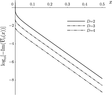
FIG. 1.: Behavior of the imaginary part of the potential: we write the quantity of (45) as $-{\mathrm{I}m}\overline{\mbox{$v$}}_{D}(x)$ and put ${\cal E}=0.1$. The imaginary part is exponentially dumping as $x$ goes larger and is smaller than $10^{-2}$ when $x>{\cal E}$. ${\mathrm{I}m}\overline{\mbox{$v$}}_{D}(0)$ is finite in $D=3$ and $D=4$ but divergent in $D=2$.

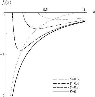
(a) (b)
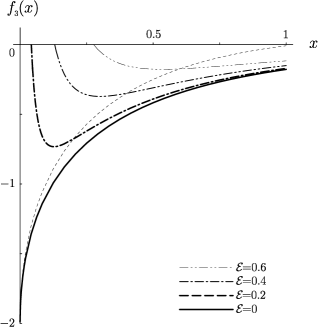
(c)

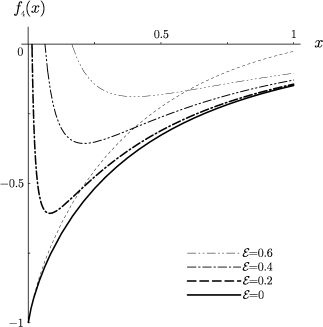
FIG. 2.: $f_{D}(x)$ for a pure electric field in (a) $D=2$, (b) $D=3$, and (c) $D=4$ for several fixed values of ${\cal E}$. In each plot, the thin-dashed line denotes $f_{D}(x)|_{{\cal E}=x}$ and shows the lower bound of $x$ (47): the vacuum is unstable in the left region to the line.

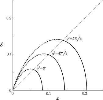
(a) (b)
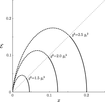
(c)

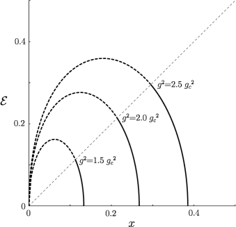
FIG. 3.: Relations between the magnitude of the electric field ${\cal E}$ and the dynamically generated mass $x$ for several fixed values of $g^{2}$ in (a) $D=2$, (b) $D=3$, and (c) $D=4$. In each plot, the thin-dashed line shows the lower bound of $x$ (47). $g_{c}^{2}$ in (b) and (c) denote the critical couplings without external fields in each dimension and are given by $\pi^{3/2}/\Lambda$ and $4\pi^{2}/\Lambda^{2}$ respectively. This shows that the mass becomes smaller when the electric field goes larger.

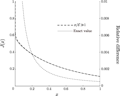
FIG. 4.: Plausibility of the asymptotic expansion in the pure electric field case: we write the integral (42) in $D=4$ as $J(x)\equiv{\cal E}\int_{1}^{\infty}\!\!d\tau\,\tau^{-2}{\mathrm{e}}^{-\tau x}\coth(\tau{\cal E})$ and put ${\cal E}=0.25$. The thin line denotes the (numerically evaluated) exact value and the dashed line represents the asymptotic expansion up to the second term. The dotted line denotes the relative difference $[(Approx.)-(Exact)]/(Exact)$ using right-hand scale. Matching is excellent for any $x$ down to ${\cal E}$.

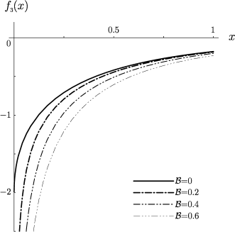
(a) (b)

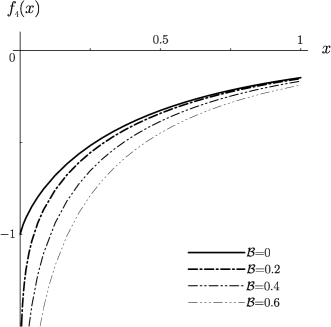
FIG. 5.: $f_{D}(x)$ for a pure magnetic field in (a) $D=3$ and (b) $D=4$ for several fixed values of ${\cal B}$. The minimum of $x$ is $\epsilon/\Lambda^{2}$ so that there exists a finite critical coupling as far as $\epsilon\neq 0$. However when $\epsilon\rightarrow 0$ critical couplings go to zero ($f_{D}(x)\rightarrow-\infty$) for any non-zero ${\cal B}$.

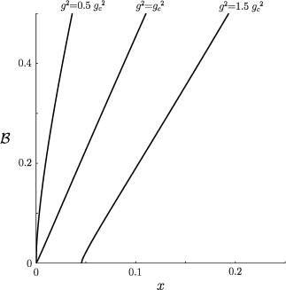
(a) (b)

FIG. 6.: Relations between the magnitude of the magnetic field ${\cal B}$ and the dynamically generated mass $x$ for several fixed values of $g^{2}$ in (a) $D=3$ and (b) $D=4$. $g_{c}^{2}$ denotes the critical couplings without external fields given by $\pi^{3/2}/\Lambda$ in 3-dimension and $4\pi^{2}/\Lambda^{2}$ in 4-dimension. This shows that a magnetic field prompts the generation of mass thus enhances $\chi$SB.

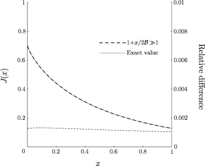
FIG. 7.: Plausibility of the improved asymptotic expansion in the pure magnetic field case: we write the integral (59) in $D=4$ as $J(x)\equiv{\cal B}\int_{1}^{\infty}\!\!d\tau\,\tau^{-2}{\mathrm{e}}^{-\tau x}\coth(\tau{\cal B})$ and put ${\cal B}=0.5$. The thin line denotes the (numerically evaluated) exact value and the dashed line represents the improved asymptotic expansion up to the first three terms. The dotted line denotes the relative difference $[(Approx.)-(Exact)]/(Exact)$. Matching is significantly excellent for all values of $x$.

(a) (b)
(c)

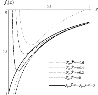
FIG. 8.: $f_{4}(x)$ for several fixed values of ${\cal F}_{\mu\nu}\widetilde{\cal F}^{\mu\nu}$ for the cases, (a) ${\cal F}_{\mu\nu}{\cal F}^{\mu\nu}=0.2$, (b) ${\cal F}_{\mu\nu}{\cal F}^{\mu\nu}=0$, and (c) ${\cal F}_{\mu\nu}{\cal F}^{\mu\nu}=-0.2$. The thick line, ${\cal F}_{\mu\nu}\widetilde{\cal F}^{\mu\nu}={\cal F}_{\mu\nu}{\cal F}^{\mu\nu}=0$, that is, no external fields, is also depicted in comparison. The thin dashed line indicates the lower bound of $x$ (83), which is obtained by putting ${\cal F}_{-}=x$ and ${\cal F}_{+}=\sqrt{x^{2}+{\cal F}_{\mu\nu}{\cal F}^{\mu\nu}/2}$ in $f_{4}(x)$. These show that ${\cal F}_{\mu\nu}\widetilde{\cal F}^{\mu\nu}$ opposes mass generation. In (a) ((c)), graphs in the physical region, satisfied with (83), are shifted to right (left) comparing to the curves in (b). This reflects the fact that in the magnetic-like case, ${\cal F}_{\mu\nu}{\cal F}^{\mu\nu}>0$, the mass goes larger while in the electric like case, ${\cal F}_{\mu\nu}{\cal F}^{\mu\nu}<0$, it goes smaller.

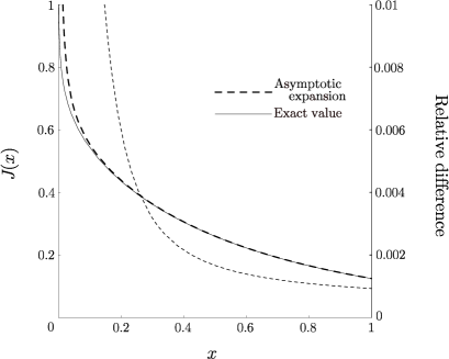
FIG. 9.: Plausibility of the asymptotic expansion for general external fields in $D=4$: we write the left-hand side of (82) as $J(x)\equiv{\cal F}_{+}{\cal F}_{-}\int_{1}^{\infty}\!\!d\tau\,\tau^{-1}{\mathrm{e}}^{-\tau x}\coth(\tau{\cal F}_{+})\coth(\tau{\cal F}_{-})$ and put ${\cal F}_{+}=0.4$ and ${\cal F}_{-}=0.2$. The thin line denotes the (numerically evaluated) exact value and the dashed line represents the asymptotic expansion in the same approximation as the one for (88). The dotted line denotes the relative difference $[(Approx.)-(Exact)]/(Exact)$. Matching is excellent for almost all values of $x$ down to ${\cal F}_{-}$.