Thermal radiation in non-static curved spacetimes: quantum mechanical path integrals and configuration space topology

Abstract

A quantum mechanical path integral derivation is given of a thermal propagator in non-static Gui spacetime. The thermal nature of the propagator is understood in terms of homotopically non-trivial paths in the configuration space appropriate to tortoise coordinates. The connection to thermal emission from collapsing black holes is discussed.

I Introduction

Path integrals can be very intuitive tools with which to tackle certain problems in quantum mechanics [1]. In the context of quantum field theory, a time-ordered two-point correlation function can be expressed as a sum over particle paths in a suitable configuration space. The usefulness of this path integral formalism stems in part from the fact that it incorporates the physically relevant boundary conditions encoding state information, and so one need not face the crucial problem of extracting the adequate solution from the propagator equation [2]. The flip side to this is that a path integral is not complete without a careful specification of the set of paths that must be summed over.

A clear advantage of the path integral formalism is that the dependence on the homotopic properties of the configuration space are explicit. Many physical phenomena, such as the Aharonov-Bohm effect, can be understood to be a consequence of these properties. Often in these cases, it is useful to work with configuration spaces that may have different topologies to that of the true physical space [3].

For an equilibrium situation, the thermal properties of a propagator are associated via the KMS condition [4] to periodicity in imaginary time. This periodicity may be enforced by expressing a thermal propagator as an infinite sum of non-thermal propagators whose time arguments are shifted as $t\to t+i\nu\hbar/(kT)$ where $\nu\in{\mathbb{Z}}$ ($\hbar$ and $k$ are the Plank and Boltzmann constants). Formally (up to the factor of $i$), this kind of expression for a thermal propagator bears a close resemblance to the propagator of a particle moving in a multiply connected configuration space. This relationship has been previously discussed in the context of Euclidean space path integrals (see for example [5]). The purpose of our work is to provide a further link between these two ideas by showing that the homotopic properties of the configuration space of a particle in curved spacetimes may be regarded as different in a Lorentzian context, in coordinates related by a non-analytic transformation. We argue that this notion of configuration space topology is closely related to the thermal properties of non-equilibrium spacetimes. We illustrate these ideas by focussing on the thermal properties of a non-static spacetime that can be regarded as a dynamical version of Gui’s $\eta-\xi$ spacetime [6].

The classic example of the path integral computation of a thermal propagator is that of the Hartle-Hawking propagator for a black hole in Schwarzschild coordinates [7]. Upon Euclideanising the Schwarzschild metric, the condition that the spacetime be free of singularities requires that the time coordinate be periodic. The periodicity leads to a thermal propagator in the obvious way. A similar conclusion can be reached in a variety of other examples after an appropriate definition of Euclidean coordinates, such as Rindler space [5] and the $\eta-\xi$ spacetime of Gui [6]. In some of these examples, it has been shown that the propagator in Euclidean space can be decomposed according to the winding of paths around a point in the Euclidean section, and that this decomposition relates the thermal propagator to a sum of non-thermal propagators [5, 6]. This decomposition can be understood in terms of homotopy if we redefine the Euclidean configuration space by removing a point.

In this paper we shall apply the path integral formalism to the thermal emission of particles in a toy model that is analogous to a collapsing black-hole spacetime. A collapsing black hole is generally treated by using the equivalence of a post-collapse hole to an eternal hole, with the additional information that the matter fields are in the Unruh vacuum at the past horizon of the eternal hole [8]. By looking at the much simpler example of a non-static Gui spacetime, we directly develop a notion of configuration space topology for different coordinates in the Lorentzian signature metric. We focus on the different homotopic properties of the configuration space of a particle viewed in either Kruskal or tortoise type coordinates in the collapse geometry. We argue that the thermal nature of the non-static Gui spacetime can be seen to follow from the non-trivial topology of the configuration space defined by tortoise coordinates if they are to cover the entire spacetime. We argue that the appropriate propagator for thermal emission is indeed obtained by considering paths that probe this non-trivial topology. This principle is demonstrated by exact calculations.

II Covariant path integrals

A The configuration space

Let us consider the general case of a particle moving freely on a curved spacetime $({\cal M},g)$. We assume that this may be parametrised entirely with a system of coordinates denoted by $q$, whose values belong to a connected manifold ${\cal Q}$, the configuration space, endowed with the metric $g_{q}$. A virtual path followed by a particle in ${\cal M}$ is given in theses coordinates by the function $q=q(\omega)$, where $\omega$ is the parameter-time. This path is denoted by $[{@,@,@,@,@,}q{@,@,@,@,@,}]$. This function is continuous everywhere except maybe at some values of $\omega$, because the coordinates $q$ may not cover ${\cal M}$ in a continuous way. In a relativistic framework, the particle is allowed to go forward and/or backwards in the time-coordinate $q^{0}$.

We shall be interested in the case where the configuration space ${\cal Q}$ is multiply connected [9]. Normally, a multiplicity of paths connecting a pair of given points in $({\cal M},g)$ is associated with the topology of the manifold ${\cal M}$. However, since the paths take values in ${\cal Q}$, it is possible that similar effects can arise when $({\cal M},g)$ is parametrised in a coordinate system that is related non-analytically to a given coordinate patch of ${\cal M}$. We shall see this explicitly below.

When the manifold $({\cal Q},g_{q})$ is multiply connected, it is useful to consider its covering space $({\widetilde{{\cal Q}}},{\tilde{g}}_{\tilde{q}})$ [9]. In this case, ${\widetilde{{\cal Q}}}$ contains many distinct images of any given point of the configuration space. The elements of the set $\Gamma$ are defined to be isometries which relate these images, so that one has ${\cal Q}={\widetilde{{\cal Q}}}/\Gamma$. The images of $q\in{\cal Q}$ will be denoted by ${\tilde{q}}^{\nu}\in{\widetilde{{\cal Q}}}$, where $\nu$ ranges over the elements of $\Gamma$. The configuration space is recovered from its connected covering space when all these images are identified. The metric ${\tilde{g}}$ in ${\widetilde{{\cal Q}}}$ is defined naturally by ${\tilde{g}}({\tilde{q}}^{\nu})=g(q)$.

Similarly, a path $[{@,@,@,@,@,}q{@,@,@,@,@,}]$ in ${\cal Q}$ has different images in ${\widetilde{{\cal Q}}}$. These are continuous functions and may be labelled according to the images of the endpoints. The base point in ${\widetilde{{\cal Q}}}$ of the endpoint $q_{i}\in{\cal Q}$ is defined by the particular image point ${\tilde{q}}_{i}\equiv{\tilde{q}}_{i}^{\nu=0}$. The paths $[{@,@,@,@,@,}{\tilde{q}}{@,@,@,@,@,}]$ with endpoints $({\tilde{q}}_{i},{\tilde{q}}_{f}^{\nu})$ belong to a given homotopy class. Paths of different classes may not be continuously deformed into one another. The set of all classes combined with a composition operator defines the fundamental group of ${\widetilde{{\cal Q}}}$.

B The propagator and the path integral

In quantum mechanics, the amplitude to move from an initial point $q_{i}\in{\cal Q}$ to a final point $q_{f}\in{\cal Q}$ in a parameter-time $s=s_{f}-s_{i}$ is given by the propagator $K_{q}(q_{i},q_{f};s)$, or heat kernel, in $q$ cordinates. It does not depend on the mass of the particle and satisfies the Schrödinger equation [10]

$$i\hbar{@,@,@,@,@,}\partial_{s}{@,@,@,@,@,}K_{q}{@,@,@,@,@,}(q^{\prime},q^{\prime\prime};s)=-\hbar^{2}{@,@,@,@,@,}\nabla^{\mu}\nabla_{\mu}{@,@,@,@,@,}K_{q}{@,@,@,@,@,}(q^{\prime},q^{\prime\prime};s),$$ (1)

where $\nabla_{\mu}$ is the covariant derivative. This propagator is related the usual propagator $G_{q}{@,@,@,@,@,}(q_{i},q_{f})$ of quantum field theory by a Fourier transform in $s$ whose conjugate variable is $m^{2}$.

Because it satisfies the Schrödinger equation (1), the propagator $K_{q}{@,@,@,@,@,}(q_{i},q_{f};s)$ can be written as a sum over paths joining the endpoints $q_{i}$ and $q_{f}$ within a parameter time $s$. In $q$ coordinates, the sum is taken over the paths contained within ${\cal Q}$, and is written symbolically as

$$K^{vac}_{q}{@,@,@,@,@,}(q_{i},q_{f};s)=\sideset{}{{}_{g_{q}}}{\sum}_{{}_{[{@,@,@,@,@,}q{@,@,@,@,@,}]\,\in\,{\cal Q}}^{q_{i}\rightarrow q_{f}}}\exp\left({@,@,@,@,@,}\frac{i}{\hbar}{@,@,@,@,@,}S_{g_{q}}{@,@,@,@,@,}[{@,@,@,@,@,}q{@,@,@,@,@,}]{@,@,@,@,@,}\right),$$ (2)

where the covariant action $S_{g_{q}}{@,@,@,@,@,}[{@,@,@,@,@,}q{@,@,@,@,@,}]$ is given by

$$S_{g}{@,@,@,@,@,}[{@,@,@,@,@,}q{@,@,@,@,@,}]=\frac{1}{4}\int_{s_{i}}^{s_{f}}\,d\omega\,g_{\mu\nu}(q)\,\dot{q}^{\mu}\,\dot{q}^{\nu}.$$ (3)

This sum over paths is defined below. With this definition, the propagator $K^{vac}_{q}{@,@,@,@,@,}(q_{i},q_{f};s)$ is a particular solution of the Schrödinger equation (1). The choice of its boundary conditions is equivalent to the choice of the configuration space ${\cal Q}$. The latter choice is natural since it is fixed by the manifold ${\cal M}$, or spacetime itself, and by the coordinates $q$. The set of paths on which the sum is taken defines actually a vacuum since, in quantum field theory, the Fourier transform $G^{vac}_{q}{@,@,@,@,@,}(q_{i},q_{f})$ of the propagator (2) is the scalar two-point correlation function in this vacuum.

The sum over paths (2) is calculated in the covering space ${\widetilde{{\cal Q}}}$. It is rewritten as sum over paths in ${\widetilde{{\cal Q}}}$ by taking into account its multiply connected topology, i.e. by summing over the classes of paths, or equivalently over the images ${\tilde{q}}_{f}^{\nu}$,

$$\sideset{}{{}_{g_{q}}}{\sum}_{{}^{q_{i}\rightarrow q_{f}}_{[{@,@,@,@,@,}q{@,@,@,@,@,}]\,\in\,{\cal Q}}}\exp\left({@,@,@,@,@,}\frac{i}{\hbar}{@,@,@,@,@,}S_{g_{q}}{@,@,@,@,@,}[{@,@,@,@,@,}q{@,@,@,@,@,}]{@,@,@,@,@,}\right)=\sum_{\nu}\ \sideset{}{{}_{{\tilde{g}}_{\tilde{q}}}}{\sum}_{{}_{[{@,@,@,@,@,}{\tilde{q}}{@,@,@,@,@,}]\,\in\,{\widetilde{{\cal Q}}}}^{{\tilde{q}}_{i}\rightarrow{\tilde{q}}_{f}^{\nu}}}\exp\left({@,@,@,@,@,}\frac{i}{\hbar}{@,@,@,@,@,}S_{{\tilde{g}}_{\tilde{q}}}{@,@,@,@,@,}[{@,@,@,@,@,}{\tilde{q}}{@,@,@,@,@,}]{@,@,@,@,@,}\right).$$ (4)

On the r.h.s. of this equation the sum is taken over paths joining the endpoints ${\tilde{q}}_{i}$ and ${\tilde{q}}_{f}^{\nu}$. It is now natural to define a propagator ${\widetilde{K}}_{\tilde{q}}$ in ${\widetilde{{\cal Q}}}$ by the sum over paths

$${\widetilde{K}}_{\tilde{q}}{@,@,@,@,@,}({\tilde{q}}^{\prime};{\tilde{q}}^{\prime\prime};s)=\sideset{}{{}_{{\tilde{g}}_{\tilde{q}}}}{\sum}_{{}^{\,{\tilde{q}}^{\prime}\rightarrow{\tilde{q}}^{\prime\prime}}_{[{@,@,@,@,@,}{\tilde{q}}{@,@,@,@,@,}]\,\in\,{\widetilde{{\cal Q}}}}}\exp\left({@,@,@,@,@,}\frac{i}{\hbar}{@,@,@,@,@,}S_{{\tilde{g}}_{\tilde{q}}}{@,@,@,@,@,}[{@,@,@,@,@,}{\tilde{q}}{@,@,@,@,@,}]{@,@,@,@,@,}\right).$$ (5)

Since the set of paths over which the sum is taken in this definition is formally different from that of Eq. (2), this propagator defines a new vacuum $vac^{\prime}$. Going back to the configuration space ${\cal Q}$, if one defines the propagator $K^{vac^{\prime}}_{q}$ through the identification ${\widetilde{K}}_{\tilde{q}}\equiv K^{vac^{\prime}}_{q}$, one obtains the result [11]

$$K^{vac}_{q}{@,@,@,@,@,}(q_{i};q_{f};s)=\sum_{\nu}K^{vac^{\prime}}_{q}{@,@,@,@,@,}({\tilde{q}}_{i};{\tilde{q}}_{f}^{\nu};s),$$ (6)

which is true in all multiply connected manifolds.

Practically, a sum over paths is calculated from a path integral. One can show that this is given by [10]

$$\sideset{}{{}_{{\tilde{g}}_{\tilde{q}}}}{\sum}_{{}^{\,{\tilde{q}}^{\prime}\rightarrow{\tilde{q}}^{\prime\prime}}_{[{@,@,@,@,@,}{\tilde{q}}{@,@,@,@,@,}]\,\in\,{\widetilde{{\cal Q}}}}}\exp\left({@,@,@,@,@,}\frac{i}{\hbar}{@,@,@,@,@,}S_{{\tilde{g}}_{\tilde{q}}}{@,@,@,@,@,}[{@,@,@,@,@,}{\tilde{q}}{@,@,@,@,@,}]{@,@,@,@,@,}\right)=\underset{[{@,@,@,@,@,}{\tilde{q}}{@,@,@,@,@,}]\,\in\,{\widetilde{{\cal Q}}}}{\int_{{\tilde{q}}^{\prime}}^{{\tilde{q}}^{\prime\prime}}}D_{{\tilde{g}}_{\tilde{q}}}{@,@,@,@,@,}[{@,@,@,@,@,}{\tilde{q}}{@,@,@,@,@,}]\,\exp\left({@,@,@,@,@,}\frac{i}{\hbar}{@,@,@,@,@,}S_{{\tilde{g}}_{\tilde{q}}}{@,@,@,@,@,}[{@,@,@,@,@,}{\tilde{q}}{@,@,@,@,@,}]\,\right).$$ (7)

If the scalar curvature vanishes, the path integral on the r.h.s. of this equation is defined by

$$\underset{[{@,@,@,@,@,}{\tilde{q}}{@,@,@,@,@,}]\,\in\,{\widetilde{{\cal Q}}}}{\int_{{\tilde{q}}^{\prime}}^{{\tilde{q}}^{\prime\prime}}}\!D_{{\tilde{g}}_{\tilde{q}}}{@,@,@,@,@,}[{@,@,@,@,@,}{\tilde{q}}{@,@,@,@,@,}]\ e^{\frac{i}{\hbar}{@,@,@,@,@,}S_{{\tilde{g}}_{\tilde{q}}}{@,@,@,@,@,}[{@,@,@,@,@,}{\tilde{q}}{@,@,@,@,@,}]}=\lim_{N\rightarrow\infty}\left(\frac{N}{4\pi\hbar is}\right)^{2N}\prod_{j=1}^{N-1}\int_{{\widetilde{{\cal Q}}}}d^{4}{\tilde{q}}_{j}\parallel\!{\tilde{g}}_{\tilde{q}}({\tilde{q}}_{j})\!\parallel^{\frac{1}{2}}e^{\frac{i}{4\hbar}{@,@,@,@,@,}\sum_{k=1}^{N}\int_{s_{k-1}}^{s_{k}}\!\!d\omega\,{\tilde{g}}_{\mu\nu}{@,@,@,@,@,}\dot{{\tilde{q}}}^{\mu}(\omega){@,@,@,@,@,}\dot{{\tilde{q}}}^{\nu}(\omega)}$$ (8)

where $s_{j}=s_{i}+js/N$, ${\tilde{q}}_{j}={\tilde{q}}(s_{j})$ ($j=0,1,...,N$), $N\in{\mathbb{N}}$ and $\parallel\ \parallel$ denotes the absolute value of the determinant. Each integral in the exponential is evaluated along the image-geodesic connecting ${\tilde{q}}_{j-1}$ and ${\tilde{q}}_{j}$ which ensures that the path integral is covariant.

III A simple model

A The non-static Gui spacetime

Let us now introduce a simple dynamical spacetime model that will allow us to perform explicit calculations. This two-dimensional model is defined by the line element [12]

$$ds^{2}_{h}=\frac{dx^{+}\,dx^{-}}{\kappa\left(x^{-}_{H}-x^{-}\,\right)},$$ (9)

where $x^{\pm}=x^{0}\pm x^{1}$, $x^{-}_{H}\in{\mathbb{R}}$ and $\kappa>0$. The $x$ coordinates are Kruskal-like coordinates. This line element is the dynamical equivalent of the eta-xi spacetime of Gui [6]. We define regions $I$ and $I\!I$ by the half-planes $x^{-}<x^{-}_{H}$ and $x^{-}>x^{-}_{H}$ respectively, see Fig. 1.

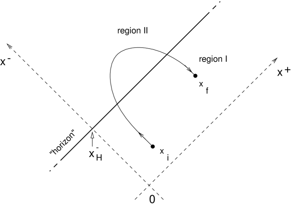
FIG. 1.: Spacetime diagram of the Gui non-static spacetime. A path crossing twice the “horizon” is shown.

Two sets of tortoise-like coordinates $y_{I}$ and $y_{I\!I}$ are defined there by

$$x^{-}(y^{-}_{I}) = x^{-}_{H}-2\exp\left[-\kappa{@,@,@,@,@,}(y^{-}_{I}-x^{-}_{H}){@,@,@,@,@,}\right],$$ (10)

$$x^{-}(y^{-}_{I\!I}) = x^{-}_{H}+2\exp\left[-\kappa{@,@,@,@,@,}(y^{-}_{I\!I}-x^{-}_{H}){@,@,@,@,@,}\right],$$ (11)

and by $x^{+}(y^{+}_{I,I\!I})=y^{+}_{I,I\!I}$. These new coordinates are actually Minkowski coordinates since we have

$$ds^{2}_{h}=dy^{+}_{a}\,dy^{-}_{a},\qquad a=I,I\!I.$$ (12)

This means that the spacetime we have defined is made of two causally and classically disconnected copies of Minkowski spacetime glued together. The null line $x^{-}=x^{-}_{H}$ will be called the “horizon”.

For this simple model, the configuration spaces ${\cal X}$ and ${\cal Y}_{a}$ ($a=I,I\!I$) in $x$ and $y$ coordinates are given by

$${\cal X} = \{\,(x^{+},x^{-})\in{\mathbb{R}}^{2}\,\},$$ (13)

$${\cal Y}_{a} = \{\,(y^{+}_{a},y^{-}_{a})\in{\mathbb{R}}^{2}\,\},\qquad a=I,I\!I,$$ (14)

and these are isomorphic to their corresponding covering spaces ${\widetilde{{\cal X}}}$ and ${\widetilde{{\cal Y}}}_{a}$, $a=I,I\!I$.

B The complex covering space and its topology

The utility of the coordinates $y_{a}$ ($a=I,I\!I$) introduced in the preceding section stems from the fact that their are Minkowskian. It then seems possible to calculate explicitly the path integral in these coordinates. However, to actually calculate a sum over paths it is necessary to work with a connected configuration space, instead for example of the two sets ${\cal Y}_{I}$ and ${\cal Y}_{I\!I}$, see Eq. (14). One needs to be able to parametrise a path crossing the “horizon" with only one set of coordinates.

Since one does not have a real set of Minkowski coordinates to cover both the regions $I$ and $I\!I$ at our disposal, we shall introduce a complex set of Minkowski coordinates denoted by $y$. These are defined in the covering space by the identifications

$${\tilde{y}}^{-}_{I} \equiv {\tilde{y}}^{-}+i2\pi\nu/\kappa,$$ (15)

$${\tilde{y}}^{-}_{I\!I} \equiv {\tilde{y}}^{-}+i2\pi(\nu+1/2)/\kappa,$$ (16)

where $\nu\in{\mathbb{Z}}$, and ${\tilde{y}}^{+}_{I,I\!I}={\tilde{y}}^{+}$. The transformations (10) and (11) may then be written together in a compact form:

$${\tilde{x}}^{-}({\tilde{y}}^{-})=x^{-}_{H}-2\exp\left[-\kappa{@,@,@,@,@,}({\tilde{y}}^{-}-x^{-}_{H}){@,@,@,@,@,}\right].$$ (17)

The necessity of allowing arbitrary integer values for $\nu$ in Eqs. (15) and (16) stems from the fact that one needs to parametrise continuously a path crossing for example several times the “horizon" as shown below. The complex covering space ${\widetilde{{\cal Y}}}$ is then given by

$${\widetilde{{\cal Y}}}=\{\,({\tilde{y}}^{+},{\tilde{y}}^{-})\in{\mathbb{R}}\times\bigcup_{\mu\,\in\,{\mathbb{Z}}}A_{\mu/2}\bigcup B\,\},$$ (18)

where $A_{\mu}={\mathbb{R}}+i2\pi\mu/\kappa$ and $B=+\infty+i{\mathbb{R}}$. The set $B$ parametrises the “horizon" and the sets $\bigcup_{\mu\,\in\,{\mathbb{Z}}}A_{\mu}$ and $\bigcup_{\mu\,\in\,{\mathbb{Z}}}A_{\mu+1/2}$ the regions $I$ and $I\!I$ respectively. The space ${\widetilde{{\cal Y}}}$ is represented in Fig. 2.

FIG. 2.: A section of the tortoise complex covering space ${\widetilde{{\cal Y}}}$ along the ${\tilde{y}}^{-}$ coordinate.

A point $y$ in ${\cal Y}$ has thus a denumerable infinite number of images in ${\widetilde{{\cal Y}}}$. These will be denoted by ${\tilde{y}}^{\nu}$, where $\nu\in{\mathbb{Z}}$, and are defined in Eqs. (15) and (16) if the point $y$ is located in the regions $I$ and $I\!I$ respectively. These images are related through an isometry of the set

$$\Gamma = \{\,\gamma_{\nu}:({\tilde{y}}^{+},{\tilde{y}}^{-})\mapsto({\tilde{y}}^{+},{\tilde{y}}^{-}+i2\pi\nu/\kappa),\,\nu\in{\mathbb{Z}}\,\}.$$ (19)

The configuration space ${\cal Y}$ is obtained by identifying them in such a way that ${\cal Y}={\widetilde{{\cal Y}}}/\Gamma$. The resulting manifold is shown in Fig. 3. Clearly, it is not simply connected. The topology of the “horizon" in the configuration space in the coordinates $(y^{+},y^{-})$ is thus that of ${\mathbb{R}}\times{\mathbb{S}}^{1}_{1/\kappa}$, where ${\mathbb{S}}^{1}_{1/\kappa}$ is a circle of radius $\kappa^{-1}$. The fact that the topologies of ${\cal X}$ and ${\cal Y}$ are different stems from the fact that the transformation (17) is not analytic.

FIG. 3.: A section of the configuration spaces a) ${\cal X}$ and b) ${\cal Y}$ along the $x^{-}$ and $y^{-}$ coordinates respectively.

The fundamental group of ${\cal Y}$ is thus isomorphic to ${\mathbb{Z}}$. The classes of paths are labelled by the integer $\nu$ which is the winding number of the paths around the circle ${\mathbb{S}}^{1}_{1/\kappa}$. A path crossing the “horizon" twice is represented in Fig. 1. Their images of winding number $+1$, $-1$ and $0$ in the covering and configuration spaces are shown in Figs. 4, 5 and 6 respectively.

FIG. 4.: A path crossing the horizon twice with winding number +1 in the a) covering space ${\widetilde{{\cal Y}}}$ and b) in the configuration space ${\cal Y}$.

FIG. 5.: A path crossing the horizon twice with winding number -1 in the a) convering space ${\widetilde{{\cal Y}}}$ and b) in the configuration space ${\cal Y}$.

FIG. 6.: A path crossing the horizon twice with winding number 0 in the a) covering space ${\widetilde{{\cal Y}}}$ and b) in the configuration space ${\cal Y}$.

C Applying the path integral formalism

We now turn to the problem of calculating the propagator from the path integral formalism. This is expressed as a sum over paths in the configuration space ${\cal X}$,

$$K^{in}_{x}(x_{i},x_{f};s)=\sideset{}{{}_{h_{x}}}{\sum}_{{}^{x_{i}\rightarrow x_{f}}_{[{@,@,@,@,@,}x{@,@,@,@,@,}]\,\in\,{\cal X}}}\exp\left({@,@,@,@,@,}\frac{i}{\hbar}{@,@,@,@,@,}S_{h_{x}}{@,@,@,@,@,}[{@,@,@,@,@,}x{@,@,@,@,@,}]{@,@,@,@,@,}\right),$$ (20)

where the metric $h_{x}$ in $x$ coordinates is given in Eq. (9). This expression defines the incoming vacuum $in$. It is difficult to calculate the sum over paths in this form, because of the presence of the non-trivial metric $h_{x}$. Our strategy is to transform it to the complex $y$ coordinates covering the entire spacetime, in which the metric is Minkowskian. The relevant connected configuration space to consider is then ${\cal Y}$. The interesting physics follows from the non-trivial topology of this configuration space as we show now.

The sum over paths (20) when written as a path integral in the covering space ${\widetilde{{\cal X}}}$ is badly defined because the metric $h_{x}$ is singular at $x^{-}=x^{-}_{H}$. The obvious way to define it correctly is to performed the integration over ${\tilde{x}}^{-}$ using the principal value. This is thus defined by

$$\sideset{}{{}_{h_{x}}}{\sum}_{{}^{x_{i}\rightarrow x_{f}}_{[{@,@,@,@,@,}x{@,@,@,@,@,}]\,\in\,{\cal X}}}\exp\left({@,@,@,@,@,}\frac{i}{\hbar}{@,@,@,@,@,}S_{h_{x}}{@,@,@,@,@,}[{@,@,@,@,@,}x{@,@,@,@,@,}]{@,@,@,@,@,}\right)=\underset{[{@,@,@,@,@,}x{@,@,@,@,@,}]\,\in\,{\widetilde{{\cal X}}}^{*}}{\int_{{\tilde{x}}_{i}}^{{\tilde{x}}_{f}}}D_{{\tilde{h}}_{\tilde{x}}}{@,@,@,@,@,}[{@,@,@,@,@,}{\tilde{x}}{@,@,@,@,@,}]\,\exp\left({@,@,@,@,@,}\frac{i}{\hbar}{@,@,@,@,@,}S_{{\tilde{h}}_{\tilde{x}}}{@,@,@,@,@,}[{@,@,@,@,@,}{\tilde{x}}{@,@,@,@,@,}]{@,@,@,@,@,}\right),$$ (21)

where the space ${\widetilde{{\cal X}}}^{*}$ is given by

$${\widetilde{{\cal X}}}^{*} = \{\,({\tilde{x}}^{+},{\tilde{x}}^{-})\in{\mathbb{R}}\times{\mathbb{R}}^{*}\,\},$$ (22)

if ${\mathbb{R}}^{*}=\lim_{\epsilon\rightarrow{0}}\,(-\infty,-\epsilon]\cup[+\epsilon,+\infty)$. Interestingly, this definition amounts to getting rid of the paths crossing the “horizon" at one or more of the parameter-time values $s_{j}$ of Eq. (8), where $j=1,...,N-1$ ($N\in{\mathbb{N}}$).

We now perform a change of coordinates in the sum over paths and because the propagator is a biscalar one may write

$$\sideset{}{{}_{h_{x}}}{\sum}_{{}^{x_{i}\rightarrow x_{f}}_{[{@,@,@,@,@,}x{@,@,@,@,@,}]\,\in\,{\cal X}}}\exp\left({@,@,@,@,@,}\frac{i}{\hbar}{@,@,@,@,@,}S_{h_{x}}{@,@,@,@,@,}[{@,@,@,@,@,}x{@,@,@,@,@,}]{@,@,@,@,@,}\right)=\sideset{}{{}_{\eta}}{\sum}_{{}^{y_{i}\rightarrow y_{f}}_{[{@,@,@,@,@,}y{@,@,@,@,@,}]\,\in\,{\cal Y}}}\exp\left({@,@,@,@,@,}\frac{i}{\hbar}{@,@,@,@,@,}S_{\eta}{@,@,@,@,@,}[{@,@,@,@,@,}y{@,@,@,@,@,}]{@,@,@,@,@,}\right).$$ (23)

Since the sum over paths on the r.h.s. is also badly defined when written as a path integral in the covering space ${\widetilde{{\cal Y}}}$, we introduce the space ${\widetilde{{\cal Y}}}^{*}$ by

$${\widetilde{{\cal Y}}}^{*}=\{\,({\tilde{y}}^{+},{\tilde{y}}^{-})\in{\mathbb{R}}\times\bigcup_{\mu\,\in\,{\mathbb{Z}}}A_{\mu/2}\,\},$$ (24)

i.e. we removed the set ${\mathbb{R}}\times B$ from ${\widetilde{{\cal Y}}}$, and we rewrite the sum over paths in the form

$$\sideset{}{{}_{\eta}}{\sum}_{{}^{y_{i}\rightarrow y_{f}}_{[{@,@,@,@,@,}y{@,@,@,@,@,}]\,\in\,{\cal Y}}}\exp\left({@,@,@,@,@,}\frac{i}{\hbar}{@,@,@,@,@,}S_{\eta}{@,@,@,@,@,}[{@,@,@,@,@,}y{@,@,@,@,@,}]{@,@,@,@,@,}\right)=\sum_{\nu\in{\mathbb{Z}}}\underset{[{@,@,@,@,@,}{\tilde{y}}{@,@,@,@,@,}]\,\in\,{\widetilde{{\cal Y}}}^{*}}{\int_{{\tilde{y}}_{i}}^{{\tilde{y}}^{\nu}_{f}}}D_{\tilde{\eta}}{@,@,@,@,@,}[{@,@,@,@,@,}{\tilde{y}}{@,@,@,@,@,}]\,\exp\left({@,@,@,@,@,}\frac{i}{\hbar}{@,@,@,@,@,}S_{\tilde{\eta}}{@,@,@,@,@,}[{@,@,@,@,@,}{\tilde{y}}{@,@,@,@,@,}]{@,@,@,@,@,}\right),$$ (25)

where ${\tilde{\eta}}=\eta$. In this last equation, we have taken into account the multiply connected nature of ${\cal Y}$ by summing over the different classes of path with winding number $\nu$. Each integral in the sum (25) of path integrals is given by

$$\int_{{\widetilde{{\cal Y}}}^{*}}\!\!d^{2}{\tilde{y}}_{j}\ e^{\frac{i}{4\hbar}\sum_{k=1}^{N}\int_{s_{k-1}}^{s_{k}}\!\!d\omega\,{\tilde{\eta}}_{\mu\nu}\,\dot{{\tilde{y}}}^{\mu}(\omega)\,\dot{{\tilde{y}}}^{\nu}(\omega)} = \sum_{\mu\in{\mathbb{Z}}}\int_{A_{\mu/2}}\!\!\!\!d{\tilde{y}}^{-}_{j}\int_{{\mathbb{R}}}\!\!\!d{\tilde{y}}^{+}_{j}\,e^{\frac{i}{4\hbar}\sum_{k=1}^{N}\int_{s_{k-1}}^{s_{k}}\!\!d\omega\,{\tilde{\eta}}_{\mu\nu}\,\dot{{\tilde{y}}}^{\mu}(\omega)\,\dot{{\tilde{y}}}^{\nu}(\omega)}.$$ (26)

Since the integrand in the r.h.s. of this last equation does not actually depend on the imaginary value of ${\tilde{y}}^{-}_{j}$, we have

$$\int_{{\widetilde{{\cal Y}}}^{*}}d^{2}{\tilde{y}}_{j}\ e^{\frac{i}{4\hbar}\sum_{k=1}^{N}\int_{s_{k-1}}^{s_{k}}\!d\omega\,{\tilde{\eta}}_{\mu\nu}\,\dot{{\tilde{y}}}^{\mu}(\omega)\,\dot{{\tilde{y}}}^{\nu}(\omega)}=C\int_{{\mathbb{R}}^{2}}d^{2}{\tilde{y}}_{j}\ e^{\frac{i}{4\hbar}\sum_{k=1}^{N}\int_{s_{k-1}}^{s_{k}}\!d\omega\,{\tilde{\eta}}_{\mu\nu}\,\dot{{\tilde{y}}}^{\mu}(\omega)\,\dot{{\tilde{y}}}^{\nu}(\omega)},$$ (27)

where $C$ is an infinite constant, which can be removed by normalising correctly the path integral to take into account the fact that the integration is made over an infinite number of copies of ${\mathbb{R}}^{2}$. The sum over paths becomes then

$$\sideset{}{{}_{g_{x}}}{\sum}_{{}^{x_{i}\rightarrow x_{f}}_{[{@,@,@,@,@,}x{@,@,@,@,@,}]\,\in\,{\cal X}}}\exp\left({@,@,@,@,@,}\frac{i}{\hbar}{@,@,@,@,@,}S_{g_{x}}{@,@,@,@,@,}[{@,@,@,@,@,}x{@,@,@,@,@,}]{@,@,@,@,@,}\right) = \sum_{\nu\in{\mathbb{Z}}}\underset{[{@,@,@,@,@,}{\tilde{y}}{@,@,@,@,@,}]\,\in\,{\mathbb{R}}^{2}}{\int_{{\tilde{y}}_{i}}^{{\tilde{y}}^{\nu}_{f}}}D_{{\tilde{\eta}}}{@,@,@,@,@,}[{@,@,@,@,@,}{\tilde{y}}{@,@,@,@,@,}]\,\exp\left({@,@,@,@,@,}\frac{i}{\hbar}{@,@,@,@,@,}S_{{\tilde{\eta}}}{@,@,@,@,@,}[{@,@,@,@,@,}{\tilde{y}}{@,@,@,@,@,}]{@,@,@,@,@,}\right).$$ (28)

It has thus been rewritten as a sum of real path integrals, although the final endpoint is complex. It is regularised by performing two Wick rotations in both the parameter-time and the time-coordinate in the standard way [13]. The contribution of the class of paths with winding number $\nu$ is the free propagator ${\widetilde{K}}_{0}$ in ${\tilde{y}}$ with arguments ${\tilde{y}}_{i}$ and ${\tilde{y}}_{f}^{\nu}$:

$$\underset{[{@,@,@,@,@,}{\tilde{y}}{@,@,@,@,@,}]\,\in\,{\widetilde{{\cal Y}}}^{*}}{\int_{{\tilde{y}}_{i}}^{{\tilde{y}}^{\nu}_{f}}}D_{\tilde{\eta}}{@,@,@,@,@,}[{@,@,@,@,@,}{\tilde{y}}{@,@,@,@,@,}]\,\exp\left({@,@,@,@,@,}\frac{i}{\hbar}{@,@,@,@,@,}S_{\tilde{\eta}}{@,@,@,@,@,}[{@,@,@,@,@,}{\tilde{y}}{@,@,@,@,@,}]{@,@,@,@,@,}\right)={\widetilde{K}}_{0}\left(\,{\tilde{y}}_{i},\,{\tilde{y}}_{f}^{\nu};\,s\,\right).$$ (29)

The outgoing vacuum is defined by ${\widetilde{K}}_{0}=K^{out}_{0}$. By adding all these propagators, the total propagator is obtained

$$K^{in}_{y}\left(\,y_{i};\,y_{f};\,s\,\right)=\sum_{\nu\in{\mathbb{Z}}}K^{out}_{0}\left(\,y_{i};\,y^{+}_{f},y^{-}_{f}+i2\pi\nu/\kappa;\,s\,\right).$$ (30)

The propagator therefore represents a right-moving thermal flux of particles with temperature $T=\hbar\kappa/(2\pi k)$, as can be shown by calculating the component $(--)$ of the energy-momentum tensor from this expression [12].

D Relation to the collapsing Schwarzschild black hole

A collapsing Schwarzschild black hole can be modelled by an imploding spherical shell of radiation. If one assumes that the shell is infinitesimally thin as did Synge [14], the only non-vanishing energy-momentum tensor component in the Kruskal coordinates $u$ is

$$T_{++}(u)=\frac{M}{4\pi r^{2}}\,\delta(u^{+}-u^{+}_{0}),$$ (31)

where $M>0$ and $u^{+}_{0}>0$. From the equations of General Relativity one obtains the line element [14]

$$ds^{2}_{g}=\left[\,1-\frac{2m(u^{+})}{r}\,\right]\,\frac{du^{+}\,du^{-}}{\left[\,1-\displaystyle\frac{4m(u^{+})}{(u^{+}_{0}-u^{-})}\,\right]}-r(u^{+},u^{-})^{2}\,d\Omega^{2},$$ (32)

where $d\Omega^{2}=d\theta^{2}+\sin^{2}\theta\,d\phi^{2}$ and $m(u^{+})=M\,\theta(u^{+}-u^{+}_{0})$. Inside the collapsing shell, one has $u^{\pm}=t\pm r$, where $t$ is the time coordinate and $r\geq 0$ the radius, and the line element is Minkowskian there. Outside the imploding shell, the Kruskal and Schwarzschild coordinates $(t,r)$ are related implicitly by

$$\exp\left(-2{@,@,@,@,@,}\kappa{@,@,@,@,@,}t\right) = |\,u^{-}_{H}-u^{-}\,|\ \exp\left[\kappa{@,@,@,@,@,}(u^{-}_{H}-u^{-}-u^{+})\right],$$ (33)

$$2\left(\,r-2M\,\right)\,\exp\left(2{@,@,@,@,@,}\kappa{@,@,@,@,@,}r\right) = \left(\,u^{-}_{H}-u^{-}\,\right)\,\exp\left[\kappa{@,@,@,@,@,}(u^{+}-u^{-})\right],$$ (34)

where $\kappa=1/(4M)$ and $u^{-}_{H}=u^{+}_{0}-4M$. The collapsing spacetime is represented in Fig. 7. The horizon is located at $u^{-}=u^{-}_{H}$ or $r=2M$ if $u^{+}>u^{+}_{0}$. The Kruskal configuration space ${\cal U}$ is given by

$${\cal U}=\{\,(u^{+},u^{-},\theta,\phi)\in{\mathbb{R}}^{2}\times{\mathbb{S}}^{2}\ |\ r(u^{+},u^{-})\geq 0\,\}.$$ (35)

It is homotopically trivial, i.e. it is isomorphic to its covering space ${\widetilde{{\cal U}}}$.

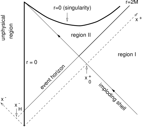
FIG. 7.: Spacetime diagram of the Synge collapse in Kruskal coordinates. Each point represents a sphere ${\mathbb{S}}^{2}$. The physical region, or accessible region of spacetime, defines the Kruskal configuration space ${\cal K}$.

Two new sets of coordinates $v_{I}$ and $v_{I\!I}$ can be defined for $u^{-}<u^{-}_{H}$ and $u^{-}>u^{-}_{H}$ respectively by

$$v^{-}_{I}(u^{-}) = u^{-}-\kappa^{-1}\,\ln\left[\,(u^{-}_{H}-u^{-}\,)/2\right],$$ (36)

$$v^{-}_{I\!I}(u^{-}) = u^{-}-\kappa^{-1}\,\ln\left[\,(u^{-}-u^{-}_{H}\,)/2\right],$$ (37)

and $v^{+}_{I,I\!I}(u^{+})=u^{+}$. The $v_{I,I\!I}$ are tortoise coordinates. Outside the shell, the line element (32) is the Schwarzschild line element in $(t,r)$ coordinates where $(v^{0}_{I,I\!I},v^{1}_{I,I\!I})=(t,r+2M\,\ln\left|\,r-2M\,\right|)$.

We will be interested in a connected region ${\cal R}$ defined by $u^{-}\approx u^{-}_{H}$ and $u^{+}\gg 1$. Within this region, there is a subregion which is located far from the black hole and at late times (i.e. $r\gg 2M$ and $t\gg 1$). This subregion is denoted by ${\overline{{\cal R}}}$. An inertial observer far from the black hole is contained within this region at late times. In ${\overline{{\cal R}}}$, the line element (32) becomes

$$ds^{2}_{g} \approx \frac{du^{+}\,du^{-}}{\kappa\left(u^{-}_{H}-u^{-}\,\right)}-r(u^{+},u^{-})^{2}\,d\Omega^{2},$$ (38)

and the transformations (36) and (37) are given if $u^{-}\approx u^{-}_{H}$ by

$$u^{-}(v^{-}_{I}) \approx u^{-}_{H}-2\exp\left[-\kappa\,(v^{-}_{I}-u^{-}_{H}){@,@,@,@,@,}\right],$$ (39)

$$u^{-}(v^{-}_{I\!I}) \approx u^{-}_{H}+2\exp\left[-\kappa\,(v^{-}_{I\!I}-u^{-}_{H}){@,@,@,@,@,}\right].$$ (40)

Under the identifications $u\equiv x$ and $v_{I,I\!I}\equiv y_{I,I\!I}$, these clearly agree formally with the metric (9) and transformations (10) and (11) of the non-static Gui spacetime, if abstraction is made of the angular degrees of freedom.

The complex tortoise coordinate $v$ is defined from the coordinates $v_{I}$ and $v_{I\!I}$ as in Eqs. (15) and (16). The tranformations (36) and (37) may then be written in the compact form

$$\exp\left(-\kappa{\tilde{v}}^{-}\right)=\frac{1}{2}\,\exp\left(-\kappa{\tilde{u}}^{-}\right)\,(u^{-}_{H}-{\tilde{u}}^{-}).$$ (41)

From this it follows that the complex points ${\tilde{v}}^{-}$ and ${\tilde{v}}^{-}+i2\pi/\kappa$ represent the same event in spacetime.

Since the configuration space in tortoise coordinates follows directly form the transformation (41), or from the transformations (39) and (40) close to the event-horizon, one can see that the homotopy of the configuration space ${\cal V}$ in the $v$ coordinates is analogous to that found above for the $y$ coordinates. The complex configuration space ${\widetilde{{\cal V}}}$ is given by

$${\widetilde{{\cal V}}}=\{\,({\tilde{v}}^{+},{\tilde{v}}^{-},{\widetilde{\Omega}})\in{\mathbb{R}}\times\left[\bigcup_{\mu\,\in\,{\mathbb{Z}}}A_{\mu/2}\cup B\right]\times{\mathbb{S}}^{2}\mbox{ such that }r(v^{+},v^{-})>0\,\},$$ (42)

where the sets $A_{\mu}$ and $B$ are defined after Eq. (18), see Fig. 8. The topology of the horizon in tortoise complex configuration space is circular, it is given by ${\mathbb{R}}\times{\mathbb{S}}^{1}_{1/\kappa}\times{\mathbb{S}}^{2}$ in the $(v^{+},v^{-},\Omega)$ coordinates, see Fig. 9.

FIG. 8.: A section of the tortoise complex covering space ${\widetilde{{\cal V}}}$ along the ${\tilde{v}}^{-}$ coordinate.

FIG. 9.: A section of the configuration spaces a) ${\cal U}$ and b) ${\cal V}$ along the $u^{-}$ and $v^{-}$ coordinates respectively.

Since the configuration space ${\widetilde{{\cal V}}}$ is invariant under the action of the transformations ${\tilde{v}}^{-}\mapsto{\tilde{v}}^{-}+i2\pi\nu/\kappa$ where $\nu\in{\mathbb{Z}}$, the propagator ${\widetilde{K}}_{v}$ satisfies

$${\widetilde{K}}_{v}\left({\tilde{v}}_{i};{\tilde{v}}^{+}_{f},{\tilde{v}}_{f}^{-}+i2\pi\nu/\kappa,{\widetilde{\Omega}}_{f};s\right)={\widetilde{K}}_{v}\left({\tilde{v}}_{i}^{+},{\tilde{v}}_{i}^{-}-i2\pi\nu/\kappa,{\widetilde{\Omega}}_{i};{\tilde{v}}_{f};s\right).$$ (43)

From Eq. (6) we obtain furthermore

$$K^{in}_{v}\left(v_{i};v_{f};s\,\right)=\sum_{\nu\in{\mathbb{Z}}}K^{out}_{v}\left(v_{i};v^{+}_{f},v^{-}_{f}+i2\pi\nu/\kappa,\Omega_{f};s\,\right).$$ (44)

These expressions are true everywhere. However, contrary to the Gui spacetime, the propagator $K^{out}_{v}$ is not a free propagator in the present case. The propagator $K^{in}_{v}$ is obviously periodic in the imaginary direction $v^{-}$,

$$K^{in}_{v}\left(v_{i};v^{+}_{f},v^{-}_{f},\Omega_{f};s\,\right)=K^{in}_{v}\left(v_{i};v^{+}_{f},v^{-}_{f}+i2\pi\nu/\kappa,\Omega_{f};s\,\right).$$ (45)

We interpret these results as indicating that an exact calculation of the two-point function in the Unruh vacuum for the collapsing black hole should include a sum over paths that probe the non-trivial topology of the tortoise coordinates.

IV Conclusions

We have shown that if tortoise type coordinates are extended across an event horizon, this extension can be carried out in a denumerable infinite number of ways, and that this construction may be used to consider a Lorentzian path integral in tortoise coordinates which includes a sum over paths that cross the horizon. Computing such a path integral in the simple case of a non-static version of the Gui spacetime, we find that the propagator given by this choice of paths to sum over is a propagator which is periodic in the null coordinate transverse to the horizon, and whose energy-momentum tensor exhibits a thermal flux. A similar propagator has been obtained in a collapsing black-hole spacetime, and we conjecture that the corresponding propagator defines the Unruh vacuum.

It is interesting to note that while in Kruskal coordinates, the main contribution to the path integral comes from the geodesics joining the two endpoints, in tortoise coordinates, the contributions of paths crossing the horizon must also be considered. In the non-static Gui spacetime, the quantum particle may cross the horizon an arbitrary number of times, even though the regions $I$ and $I\!I$ are classically causally disconnected.

We conclude that the homotopic properties of the configuration space are not an intrinsic feature of a spacetime, but depend on the set of coordinates chosen to cover it, and may be hidden in the complex nature of coordinate relations across horizons. These properties have no physical consequences for the classical motion of a particle. However, in a quantum mechanical framework, a particle may tunnel across a horizon, and the topology of the whole configuration space is then physically relevant. We conjecture that the thermal nature of event horizons can be derived by using the fact that there is a denumerably infinite number of ways for a particle to tunnel through the horizon. These are defined by the winding number of the particle paths around the horizon in the tortoise configuration space.

- [1] R. P. Feynman and A. R. Hibbs, Quantum mechanics and path integrals (McGraw-Hill Book Co., New York, 1965); L. S. Schulman, Techniques and application of path integrals (John Wiley and Sons, New York, 1981).
- [2] C. DeWitt-Morette, A. Maheshwari and B. Nelson, Phys. Rep. 50, 255 (1979).
- [3] L. S. Schulman, Phys. Rev. 176, 1558 (1968); J. Math. Phys. 12, 304 (1971); J. S. Dowker, J. Phys. A: Gen. Phys. 5, 936 (1972).
- [4] R. Kubo, J. Phys. Soc. Jpn. 12, 570 (1957); P. C. Martin and J. Schwinger, Phys. Rev. 115, 1342 (1959).
- [5] W. Troost and H. Van Dam, Phys. Lett. B 71, 149 (1977); Nucl. Phys. B 152, 442 (1979).
- [6] Y.-X. Gui, Phys. Rev. D 42, 1988 (1990); Phys. Rev. D 46, 1869 (1992).
- [7] J. B. Hartle and S. W. Hawking, Phys. Rev. D 13, 2188 (1976).
- [8] S. W. Hawking, Commun. Math. Phys. 43, 199 (1975).
- [9] M. Lachièze-Rey and J.-P. Luminet, Phys. Rep. 254, 136 (1995).
- [10] J. D. Bekenstein and L. Parker, Phys. Rev. D 23, 2850 (1981); L. Parker, in Recent developments in gravitation, Cargèse 1978, edited by M. Lévy and S. Deser (Plenum Press, New York, 1979).
- [11] J. S. Dowker, J. Phys. A 5, 936 (1972); M. S. Marinov, Phys. Rep. 60, 1 (1980).
- [12] F. Vendrell, Helv. Phys. Acta 70, 598 (1997).
- [13] J. J. Halliwell and M. E. Ortiz, Phys. Rev. D 48, 748 (1993).
- [14] J. L. Synge, Proc. Roy. Irish Acad. 59 A, 1 (1957).