IASSNS-HEP-97/80

hep-th/9707160

July 1997

Strong/Weak Coupling Duality Relations for Non-Supersymmetric String Theories
Julie D. Blum  and  Keith R. Dienes
School of Natural Sciences, Institute for Advanced Study
Olden Lane, Princeton, N.J.  08540  USA

Both the supersymmetric $SO(32)$ and $E_{8}\times E_{8}$ heterotic strings in ten dimensions have known strong-coupling duals. However, it has not been known whether there also exist strong-coupling duals for the non-supersymmetric heterotic strings in ten dimensions. In this paper, we construct explicit open-string duals for the circle-compactifications of several of these non-supersymmetric theories, among them the tachyon-free $SO(16)\times SO(16)$ string. Our method involves the construction of heterotic and open-string interpolating models that continuously connect non-supersymmetric strings to supersymmetric strings. We find that our non-supersymmetric dual theories have exactly the same massless spectra as their heterotic counterparts within a certain range of our interpolations. We also develop a novel method for analyzing the solitons of non-supersymmetric open-string theories, and find that the solitons of our dual theories also agree with their heterotic counterparts. These are therefore the first known examples of strong/weak coupling duality relations between non-supersymmetric, tachyon-free string theories. Finally, the existence of these strong-coupling duals allows us to examine the non-perturbative stability of these strings, and we propose a phase diagram for the behavior of these strings as a function of coupling and radius.

1 Introduction and Overview

1.1 Why find duals of non-supersymmetric strings?

During the past several years, significant advances have taken place in our understanding of the strong-coupling behavior of string theory. Perhaps the biggest surprise was the fundamental conjecture that the strong-coupling behavior of certain string theories can be described as the weak-coupling behavior of corresponding “dual” theories which, in many cases, are also string theories. This observation makes it possible to address numerous non-perturbative questions which have, until now, been beyond reach.

Among these dualities, those describing the strong-coupling behavior of the supersymmetric ten-dimensional heterotic string theories play a central role. In ten dimensions, there are only two supersymmetric heterotic string theories: these are the $SO(32)$ theory, and the $E_{8}\times E_{8}$ theory. As is well-known, the $SO(32)$ heterotic theory is believed to be dual to the $SO(32)$ Type I theory [1, 2], and the $E_{8}\times E_{8}$ theory is believed to be dual to a theory whose low-energy limit is eleven-dimensional supergravity [3]. Given this information, much has been learned about the strong-coupling behavior of supersymmetric heterotic strings.

There are, however, additional heterotic string theories in ten dimensions. These strings are non-supersymmetric, and while the majority of them are tachyonic, one of them is tachyon-free. The question then arises: does this tachyon-free string have a dual theory as well? More generally, one can even ask whether the tachyonic heterotic strings might have duals.

There are numerous reasons why this is an important issue. One fundamental reason, of course, is to shed light on the structure of string duality itself. Is duality a property of supersymmetry or of supersymmetric string theory, or is it, more generally, a property of string theory independently of supersymmetry? Knowing the answer to this question might tell us the extent to which we expect these duality relations to survive supersymmetry breaking.

Another fundamental reason is perhaps the most obvious: to give possible insight into the strong-coupling non-perturbative behavior of non-supersymmetric strings. In some sense, these strings are much harder to analyze, yet their phenomenology, freed from the tight constraints of supersymmetry, might be far richer. Indeed, one might even imagine that our non-supersymmetric world is described by a non-supersymmetric string theory in which spacetime supersymmetry is broken by an analogue of the Scherk-Schwarz mechanism [4] and in which various unexpected stringy effects maintain finiteness, stabilize the gauge hierarchy, and even ensure successful gauge-coupling unification. Various proposals in this direction can be found in Refs. [5, 6, 7, 8, 9, 10]. However, because they have non-vanishing one-loop cosmological constants, these string theories are not believed to be stable, and are presumed to flow to other points in moduli space at which stability is restored. Unfortunately, an analysis of this question has been beyond reach because the non-perturbative properties of these string theories have been, until now, unknown.

Finally, one might even imagine that such studies could yield a new method of supersymmetry breaking. Indeed, if the duals of non-supersymmetric strings were somehow found to be supersymmetric, then, viewing the duality relation in reverse, one would have found a supersymmetric string theory which manages to break supersymmetry at strong coupling.

What are the non-supersymmetric ten-dimensional heterotic string models? Like their supersymmetric $SO(32)$ and $E_{8}\times E_{8}$ counterparts, there are only a limited number of such non-supersymmetric heterotic strings. These have been classified [11], and are as follows:

• a tachyon-free $SO(16)\times SO(16)$ model [12, 13];

• a tachyonic $SO(32)$ model [13, 14];

• a tachyonic $SO(8)\times SO(24)$ model [13];

• a tachyonic $U(16)$ model [13];

• a tachyonic $SO(16)\times E_{8}$ model [13, 14];

• a tachyonic $(E_{7})^{2}\times SU(2)^{2}$ model [13]; and

• a tachyonic $E_{8}$ model [11].

In all but the last case, the gauge symmetries are realized at affine level one. In Fig. 1, we show how these seven models are related to the supersymmetric $SO(32)$ and $E_{8}\times E_{8}$ models through $\mathchoice{\hbox{\cmss Z\kern-3.99994ptZ}}{\hbox{\cmss Z\kern-3.99994ptZ}}{\lower 0.9pt\hbox{\cmsss Z\kern-2.79996ptZ}}{\lower 1.2pt\hbox{\cmsss Z\kern-2.79996ptZ}}_{2}$ orbifold relations that break spacetime supersymmetry.

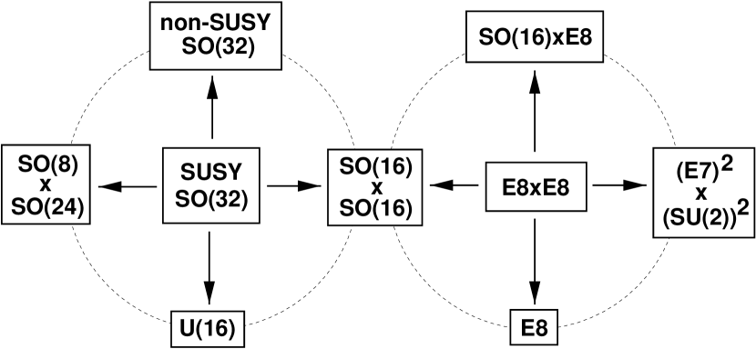
Figure 1: The relation between the seven non-supersymmetric heterotic string models in ten dimensions and the supersymmetric $SO(32)$ and $E_{8}\times E_{8}$ string models. Each arrow indicates a $\mathchoice{\hbox{\cmss Z\kern-3.99994ptZ}}{\hbox{\cmss Z\kern-3.99994ptZ}}{\lower 0.9pt\hbox{\cmsss Z\kern-2.79996ptZ}}{\lower 1.2pt\hbox{\cmsss Z\kern-2.79996ptZ}}_{2}$ orbifold relation that breaks spacetime supersymmetry. Only the tachyon-free $SO(16)\times SO(16)$ string can be realized as a $\mathchoice{\hbox{\cmss Z\kern-3.99994ptZ}}{\hbox{\cmss Z\kern-3.99994ptZ}}{\lower 0.9pt\hbox{\cmsss Z\kern-2.79996ptZ}}{\lower 1.2pt\hbox{\cmsss Z\kern-2.79996ptZ}}_{2}$ orbifold of both the supersymmetric $SO(32)$ string and the $E_{8}\times E_{8}$ string.

In this paper, we shall undertake the task of deriving strong-coupling duals for some of these non-supersymmetric theories. Throughout, we shall primarily concentrate on the case of the non-supersymmetric $SO(16)\times SO(16)$ string. Since this is the unique non-supersymmetric heterotic string which is tachyon-free, it may be expected to have special strong-coupling properties. Indeed, as is evident from Fig. 1, this string occupies a rather special, central position among the non-supersymmetric string theories, and thus its dual theory can be expected to do so as well.

After completing our analysis for the $SO(16)\times SO(16)$ case, we will then apply our techniques to some of the other non-supersymmetric ten-dimensional heterotic models listed above. Even though these models are tachyonic, we shall nevertheless find that a similar analysis can be performed, and that suitable duals can be constructed. However, our analysis will show that these tachyonic strings have a completely different stability behavior at strong coupling. Our results for these strings will therefore serve to underline the unique role of the tachyon-free $SO(16)\times SO(16)$ string.

1.2 Our approach

Of course, finding the duals of non-supersymmetric strings is not a simple undertaking, for many of the techniques that have been exploited in finding evidence for supersymmetric duality relations no longer apply when supersymmetry is absent. For example, there do not a priori exist any special non-supersymmetric string states (the analogues of BPS-saturated states) whose masses are protected against strong-coupling effects. Likewise, upon compactification, the moduli spaces of non-supersymmetric strings are not nearly as well understood as their supersymmetric counterparts.

One natural idea for deriving duals of the non-supersymmetric theories might be to start with the duals of the supersymmetric $SO(32)$ or $E_{8}\times E_{8}$ theories, and then to duplicate the action of the appropriate $\mathchoice{\hbox{\cmss Z\kern-3.99994ptZ}}{\hbox{\cmss Z\kern-3.99994ptZ}}{\lower 0.9pt\hbox{\cmsss Z\kern-2.79996ptZ}}{\lower 1.2pt\hbox{\cmsss Z\kern-2.79996ptZ}}_{2}$ orbifolds on these dual theories. Unfortunately, since these orbifolds break supersymmetry, they need not necessarily commute with strong/weak coupling duality. This issue has been discussed in Ref. [15]. Indeed, in some sense, the fundamental problem associated with this approach is that orbifold relations are discrete: one is dealing either with the original theory or with the orbifolded final theory. One cannot examine how, and where, the duality relation might begin to go wrong in passing between the original and final theories.

Therefore, in order to derive strong-coupling duals of these non-supersymmetric strings, our approach will be to relate the non-supersymmetric heterotic strings to the supersymmetric heterotic strings via continuous deformations. Since the duals for the supersymmetric theories are known, it is then hoped that one can continuously deform both sides of such supersymmetric duality relations in order to obtain non-supersymmetric duality relations. Moreover, if the duality relation were to fail to commute with such a continuous deformation, we would expect to see explicitly how and at what point this failure arises as a function of the deformation parameter.

While such continuous deformations do not exist in ten dimensions, it turns out that such deformations can indeed be performed in nine dimensions. Specifically, we shall show that it is possible to construct nine-dimensional interpolating models by compactifying ten-dimensional models on a circle of radius $R$ with a twist in such a way that a given interpolating model reproduces a ten-dimensional supersymmetric model as $R\to\infty$ and a ten-dimensional non-supersymmetric model as $R\to 0$. Such interpolating models are similar to those considered a decade ago in Refs. [16, 17, 18]. For example, one of the nine-dimensional interpolating models that we shall construct reproduces the supersymmetric $SO(32)$ heterotic string model as $R\to\infty$, but yields the $SO(16)\times SO(16)$ model as $R\to 0$. Thus, since the strong-coupling dual of the heterotic $SO(32)$ string model is believed to be the $SO(32)$ Type I model, it is natural to expect that there will be a corresponding nine-dimensional continuous deformation of the $SO(32)$ Type I model which would produce a candidate dual for the heterotic $SO(16)\times SO(16)$ model.

In order to analyze the potential continuous deformations of Type I models, it turns out to be easier to analyze the continuous deformations of the closed Type II models from which they are realized as orientifolds. Specifically, in the case of the $SO(32)$ Type I model, we would seek a continuous nine-dimensional deformation of the Type IIB model. As we shall see, there indeed exists an analogous deformation of the Type IIB model which breaks supersymmetry. This deformation is described by a nine-dimensional Type II interpolating model which connects the Type IIB model at $R\to\infty$ with the non-supersymmetric so-called Type 0B model at $R\to 0$. This situation is illustrated in Fig. 2.

Figure 2: Proposed method for deriving the dual of the heterotic $SO(16)\times SO(16)$ string model through continuous deformations away from the supersymmetric $SO(32)$ string model. Analogous deformations exist on both the heterotic and the Type II sides, from which corresponding Type I deformations can be obtained through orientifolding.

At first glance, the question would then appear to simply boil down to determining the orientifold of the Type 0B model that is produced at $R\to 0$. In fact, all possible orientifolds of the Type 0B model have been derived [19]: the resulting non-supersymmetric Type I models are found to have gauge groups of total rank $32$ rather than $16$, and (except in one case) have tachyons in their spectra. Unfortunately, while these Type I theories are interesting (and one of them has recently been conjectured [20] to be the strong-coupling dual of the bosonic string compactified to ten dimensions), their large rank precludes their identification as the duals of the non-supersymmetric heterotic strings.

We shall therefore follow a slightly different course. Rather than take the limit $R\to 0$ before orientifolding, we shall perform our orientifold directly in nine dimensions, at arbitrary radius. This will then yield a set of “interpolating” Type I models directly in nine dimensions, formulated at arbitrary radius $R$.

As we shall show, these non-supersymmetric nine-dimensional interpolating Type I models can be viewed as the strong-coupling duals of our non-supersymmetric nine-dimensional interpolating heterotic models. Specifically, for certain ranges of the radius $R$, we shall find that

• both the heterotic and Type I interpolating models are non-supersymmetric and tachyon-free;

• their massless spectra coincide exactly; and

• the D1-brane soliton of the non-supersymmetric Type I theory yields the worldsheet theory of the corresponding non-supersymmetric heterotic string.

Moreover, because of the nature of these interpolating models,

• we can smoothly take the limit as $R\to\infty$ in order to reproduce the known supersymmetric $SO(32)$ heterotic/Type I duality.

Taken together, then, this provides strong evidence for the dual relation between these non-supersymmetric string models.

As it turns out, taking the opposite limit as $R\to 0$ involves some subtleties, and we do not expect our duality relations to be valid in that limit. Thus, we have not found a strong-coupling dual for the ten-dimensional $SO(16)\times SO(16)$ string; rather, we have found a strong-coupling dual for the ($T$-dual of the) twisted compactification of this string on a circle of radius $R$, valid only for $R$ taking values within a certain range. A similar situation holds for each of the other non-supersymmetric strings we will be discussing.

As far as we are aware, our results imply the first known duality relations between non-supersymmetric, tachyon-free theories. Furthermore, as we shall see, our derivation of the Type I soliton is rather involved. In some respects, the standard derivation [22, 2] of the Type I soliton in the supersymmetric $SO(32)$ case is facilitated by the fact that the heterotic $SO(32)$ theory factorizes into separate left- and right-moving components. This crucial property is true of all supersymmetric string theories in ten dimensions, and makes it relatively straightforward to realize such heterotic theories as Type I solitons. In the present non-supersymmetric case, by contrast, the heterotic strings do not factorize so neatly, and consequently a more intricate analysis is required. Thus, we consider our derivation of this non-supersymmetric soliton — as well as our derivation of the techniques involved — to be another primary result of this paper. Indeed, we shall see that the successful matching of the soliton to the heterotic string is due in large part to certain “miracles” that are involved in these interpolating models.

Given these non-supersymmetric duality relations, we then address several of the questions raised earlier. Specifically, with our dual theories in hand, we then consider the non-perturbative stability for each of our candidate dual theories. In this way, we are able to make some conjectures concerning the ultimate fate of each of the ten-dimensional non-supersymmetric heterotic strings.

1.3 Outline of this paper

This paper is organized as follows. In Sect. 2, we provide a brief review of some of the non-supersymmetric heterotic string models that we shall be considering. Then, in Sect. 3, we shall present our interpolating models, and discuss how they are constructed. In Sect. 4, we shall focus on the interpolation of the non-supersymmetric $SO(16)\times SO(16)$ string, and construct its Type I dual. We shall then proceed to discuss the soliton of this Type I theory in Sect. 5. In Sect. 6, we then apply our techniques to some of the other non-supersymmetric heterotic string models, and in Sect. 7 we use our duality relations in order to study the perturbative and non-perturbative stability of these interpolating models. Sect. 8 then contains our conclusions, as well as a proposed phase diagram for our non-supersymmetric string models and speculations about lower-dimensional theories. Finally, in an Appendix we present the explicit free-fermionic realizations of many of the ten- and nine-dimensional models we shall be considering in this paper. Note that a brief summary of some of the results of this paper can be found in Ref. [23].

2 Review of Ten-Dimensional Models

We begin by reviewing some of the ten-dimensional heterotic and Type II string models that will be relevant for our analysis. For notational convenience, in Sects. 2–5 we shall limit our attention to the five heterotic models in Fig. 1 whose gauge groups contain $SO(16)\times SO(16)$ as a subgroup. In addition to the supersymmetric $SO(32)$ and $E_{8}\times E_{8}$ models, these include the non-supersymmetric $SO(32)$, $SO(16)\times SO(16)$, and $SO(16)\times E_{8}$ models.

Since much of our analysis of these models will proceed via their partition functions, we begin by establishing some general conventions and notation.

2.1 Conventions

Throughout this paper, we shall express partition functions in terms of the characters of the corresponding level-one affine Lie algebras. It turns out that we shall only need to consider the $SO(2n)$ gauge groups, which have central charge $c=n$ at level one. For such groups, the only level-one unitary representations are the identity (I), the vector (V), and the spinor (S) and conjugate spinor (C). This is equivalent to the statement that $SO(2n)$ has four conjugacy classes. These representations have multiplicities $\{1,2n,2^{n-1},2^{n-1}\}$ respectively, and have conformal dimensions $\{h_{I},h_{V},h_{S},h_{C}\}=\{0,1/2,n/8,n/8\}$. Their characters can then be expressed in terms of the Jacobi $\vartheta$ functions as follows:

$$\chi_{I} = {\textstyle{1\over 2}}\,({\vartheta_{3}}^{n}+{\vartheta_{4}}^{n})/\eta^{n}~{}=~{}q^{h_{I}-c/24}\,(1+n(2n-1)\,q+...)$$

$$\chi_{V} = {\textstyle{1\over 2}}\,({\vartheta_{3}}^{n}-{\vartheta_{4}}^{n})/\eta^{n}~{}=~{}q^{h_{V}-c/24}\,(2n+...)$$

$$\chi_{S} = {\textstyle{1\over 2}}\,({\vartheta_{2}}^{n}+{\vartheta_{1}}^{n})/\eta^{n}~{}=~{}q^{h_{S}-c/24}\,(2^{n-1}+...)$$

$$\chi_{C} = {\textstyle{1\over 2}}\,({\vartheta_{2}}^{n}-{\vartheta_{1}}^{n})/\eta^{n}~{}=~{}q^{h_{C}-c/24}\,(2^{n-1}+...)~{}$$ (2.1)

where $q\equiv e^{2\pi i\tau}$. Note that $n(2n-1)$ is the dimension of the adjoint representation of $SO(2n)$. This reflects the general fact that the adjoint is the first descendant of the identity field in such affine Lie algebra conformal field theories. Even though the spinor and conjugate spinor representations are distinct, we find that $\chi_{S}=\chi_{C}$ (due to the fact that $\vartheta_{1}=0$). For the ten-dimensional little Lorentz group $SO(8)$, the distinction between $S$ and $C$ is equivalent to relative spacetime chirality.

We can now express the partition functions of our string models in terms of these characters. This will also be useful for determining the massless spectra of these models. For convenience, we shall henceforth adopt the convention that all left-moving (unbarred) $\vartheta$-functions will be written in terms of the characters of $SO(16)$, while those that are right-moving (barred) will be written in terms of those of the Lorentz group $SO(8)$. Occasionally we shall also use the notation $\tilde{\chi}$ to signify left-moving $SO(32)$ characters. Furthermore, we shall define

$$Z^{(n)}_{\rm boson}~{}\equiv~{}{\tau_{2}}^{-n/2}\,({\overline{\eta}}\eta)^{-n}~{},$$ (2.2)

which represents the contribution of $n$ transverse bosons to the total partition function. Finally, we shall also define the Jacobi factor

$$\overline{J}~{}\equiv~{}{\textstyle{1\over 2}}\,\overline{\eta}^{\,-4}\,\left({\overline{\vartheta}_{3}}^{4}-{\overline{\vartheta}_{4}}^{4}-{\overline{\vartheta}_{2}}^{4}-{\overline{\vartheta}_{1}}^{4}\right)~{}=~{}\overline{\chi}_{V}-\overline{\chi}_{S}~{}=~{}0~{}.$$ (2.3)

This factor $J$ vanishes as the result of the “abstruse” identity of Jacobi, or equivalently as a result of $SO(8)$ triality, under which the $SO(8)$ vector and spinor representations are indistinguishable. Partition functions that are proportional to $J$ therefore correspond to string models with spacetime supersymmetry.

2.2 Supersymmetric $SO(32)$ string model

Given this notation, we begin by examining the supersymmetric $SO(32)$ string model. In terms of the characters $\tilde{X}$ of $SO(32)$ for the left-movers and the characters $\overline{\chi}$ $SO(8)$ for right-movers, its partition function takes the form

$$Z_{SO(32)}~{}=~{}Z^{(8)}_{\rm boson}~{}(\overline{\chi}_{V}-\overline{\chi}_{S})\,(\tilde{\chi}_{I}+\tilde{\chi}_{S})~{}.$$ (2.4)

In terms of the characters of $SO(16)\times SO(16)$ for the left-movers, this partition function is equivalent to

$$Z_{SO(32)}~{}=~{}Z^{(8)}_{\rm boson}~{}(\overline{\chi}_{V}-\overline{\chi}_{S})\,(\chi_{I}^{2}+\chi_{V}^{2}+\chi_{S}^{2}+\chi_{C}^{2})~{}.$$ (2.5)

Note that it makes no physical difference whether ${\overline{\chi}}_{S}$ or ${\overline{\chi}}_{C}$ is written in this partition function since all spinors in this model have the same spacetime chirality.

It is clear that this model is supersymmetric. It is also straightforward to determine from this partition function that the gauge group is $SO(32)$, since the massless gauge bosons in this model can only contribute to terms of the form $\overline{\chi}_{V}\times\{h=1\}$. In this partition function, the only such terms are ${\overline{\chi}}_{V}\tilde{\chi}_{I}$ or ${\overline{\chi}}_{V}\,(\chi_{I}^{2}+\chi_{V}^{2})$ where we must consider the first excited state within $\tilde{\chi}_{I}$ (in order to produce $h=1$) or equivalently the first excited state within $\chi_{I}^{2}$ and the ground state of $\chi_{V}^{2}$ (which already has $h=1$). However, the first descendant representation within $\tilde{\chi}_{I}$ is the adjoint of $SO(32)$. Equivalently, the first excited state within $\chi_{I}^{2}$ transforms as $({\bf adj,1})\oplus({\bf 1,adj})$ under $SO(16)\times SO(16)$, while the ground state of $\chi_{V}^{2}$ transforms as $({\bf vec,vec})$. Thus, under $SO(16)\times SO(16)$, the the gauge bosons of this model

$$({\bf adj,1})\oplus({\bf 1,adj})\oplus({\bf vec,vec})~{},$$ (2.6)

which fill out the 496 states of the adjoint of $SO(32)$.

It is also clear from this partition function that in addition to the gravity supermultiplet, the gauge bosons and their superpartners are the only states in the massless spectrum.

2.3 $E_{8}\times E_{8}$ string model

The partition function of the $E_{8}\times E_{8}$ model can likewise be written in terms of the $SO(16)$ characters for the left-movers, yielding

$$Z_{E_{8}\times E_{8}}~{}=~{}Z^{(8)}_{\rm boson}~{}({\overline{\chi}}_{V}-{\overline{\chi}}_{S})~{}(\chi_{I}+\chi_{S})^{2}~{}.$$ (2.7)

Once again, supersymmetry is manifest. Moreover, we immediately recognize that the level-one $E_{8}$ character is

$$\chi_{E_{8}}~{}\equiv~{}{\textstyle{1\over 2}}\,\eta^{-8}\,\left({\vartheta_{1}}^{8}+{\vartheta_{2}}^{8}+{\vartheta_{3}}^{8}+{\vartheta_{4}}^{8}\right)~{}=~{}\chi_{I}+\chi_{S}~{},$$ (2.8)

which verifies that the gauge group of this model is indeed $E_{8}\times E_{8}$. For $h=1$, the statement (2.8) reflects the fact that the adjoint plus spinor representations of $SO(16)$ combine to fill out the adjoint representation of $E_{8}$. (Note that there is only one character of $E_{8}$ because the identity is only unitary representation of $E_{8}$ at affine level one, or equivalently because $E_{8}$ has only one conjugacy class.) As with the $SO(32)$ model, we see that the gauge bosons, their superpartners, and the gravity supermultiplet are the only states in the massless spectrum.

2.4 $SO(16)\times SO(16)$ model

Next, we turn to the $SO(16)\times SO(16)$ model which will be, in large part, the main focus of this paper. In terms of the characters of $SO(16)$ for the left-movers (and those of $SO(8)$ for the right-movers), the partition function of this model takes the form

$$Z~{}=~{}Z^{(8)}_{\rm boson}~{}\times \biggl{\{} {\overline{\chi}}_{I}\,(\chi_{V}\chi_{C}+\chi_{C}\chi_{V})~{}+~{}{\overline{\chi}}_{V}\,(\chi_{I}^{2}+\chi_{S}^{2})$$ (2.9)

$$-~{}{\overline{\chi}}_{S}\,(\chi_{V}^{2}+\chi_{C}^{2})~{}-~{}{\overline{\chi}}_{C}\,(\chi_{I}\chi_{S}+\chi_{S}\chi_{I})~{}\biggr{\}}~{}.$$

It is immediately clear that supersymmetry is broken, and that the gauge group of this model is simply $SO(16)\times SO(16)$. In addition to the gravity multiplet, the complete massless spectrum of this model consists of the following $SO(16)\times SO(16)$ representations:

$${\rm vectors}: ({\bf 120},{\bf 1})\oplus({\bf 1},{\bf 120})$$

$${\rm spinors}: ({\bf 16},{\bf 16})_{+}\oplus({\bf 128},{\bf 1})_{-}\oplus({\bf 1},{\bf 128})_{-}$$ (2.10)

Here the spinor subscripts $\pm$ indicate $SO(8)$ spinors and conjugate spinors respectively; only the relative chirality between these two groups of spinors is physically relevant. Thus cancellation of the irreducible gravitational anomaly is manifest, even though supersymmetry is absent. (The other irreducible anomalies can be shown to cancel as well.) Furthermore, it is also clear that no physical tachyonic states are present in this model. In order to see this from the partition function, note that such physical tachyonic states would have to contribute to terms of the form ${\overline{\chi}}_{I}\times\{h=1/2\}$. The only possible term of this form would be ${\overline{\chi}}_{I}\,(\chi_{I}\chi_{V}+\chi_{V}\chi_{I})$, yet no such term appears in the partition function.

This model is the unique tachyon-free non-supersymmetric heterotic string model in ten dimensions. As such, we may expect it to have a number of special properties. For example, we have already seen in Fig. 1 that it is the only heterotic non-supersymmetric model in ten dimensions which can be realized as a $\mathchoice{\hbox{\cmss Z\kern-3.99994ptZ}}{\hbox{\cmss Z\kern-3.99994ptZ}}{\lower 0.9pt\hbox{\cmsss Z\kern-2.79996ptZ}}{\lower 1.2pt\hbox{\cmsss Z\kern-2.79996ptZ}}_{2}$ orbifold of either the supersymmetric $SO(32)$ model or the $E_{8}\times E_{8}$ model. Likewise, because it is tachyon-free, it is the only non-supersymmetric ten-dimensional string model to have a finite but non-vanishing one-loop cosmological constant.

Another remarkable property of the $SO(16)\times SO(16)$ string concerns its distribution of bosonic and fermionic states at all mass levels. In this string model, one has a surplus of 2112 fermionic states over bosonic states at the massless level. This reflects the broken supersymmetry. However, this surplus of fermionic states at the massless level is balanced by a surplus of 147,456 bosonic states at the first excited level (for which $L_{0}=\overline{L_{0}}=1/2$), and this is balanced in turn by a surplus of 4,713,984 fermionic states at the next excited level (for which $L_{0}=\overline{L_{0}}=1$). This pattern then continues all the way through the infinite towers of massive string states, and is illustrated in Fig. 3 where we plot the sizes of these surpluses as a function of the spacetime mass $M^{2}=2(L_{0}+\overline{L_{0}})/\alpha^{\prime}$.

Figure 3: Alternating boson/fermion surpluses in the $D=10$ non-supersymmetric tachyon-free $SO(16)\times SO(16)$ heterotic string. For each mass level $\alpha^{\prime}M_{2}\in 2\mathchoice{\hbox{\cmss Z\kern-3.99994ptZ}}{\hbox{\cmss Z\kern-3.99994ptZ}}{\lower 0.9pt\hbox{\cmsss Z\kern-2.79996ptZ}}{\lower 1.2pt\hbox{\cmsss Z\kern-2.79996ptZ}}$ in this model, we plot $\pm\log_{10}(|B_{M}-F_{M}|)$ where $B_{M}$ and $F_{M}$ are respectively the numbers of spacetime bosonic and fermionic states at that level. The overall sign is chosen positive if $B_{M}>F_{M}$, and negative otherwise. The points are connected in order to stress the alternating, oscillatory behavior of the boson and fermion surpluses throughout the string spectrum. These oscillations insure that ${{\rm Str}\,}M^{0}={{\rm Str}\,}M^{2}={{\rm Str}\,}M^{4}={{\rm Str}\,}M^{6}=0$ in this model, even though there is no spacetime supersymmetry.

These oscillations are the signature of a hidden so-called “misaligned supersymmetry” [5] in the string spectrum. Misaligned supersymmetry is a general feature of non-supersymmetric string models, and serves as the way in which string theory manages to maintain finiteness even without spacetime supersymmetry. Moreover, for tachyon-free string models, there is an added bonus: these oscillating surpluses are even sufficient to cause certain mass supertraces to vanish when evaluated over the entire string spectrum. Specifically, if one defines a regulated string supertrace via

$${{\rm Str}\,}M^{2\beta}~{}\equiv~{}\lim_{y\to 0}\,\sum_{\rm states}\,(-1)^{F}\,M^{2\beta}\,e^{-y\alpha^{\prime}M^{2}}~{},$$ (2.11)

then in ten dimensions it can be shown [6] that

$${{\rm Str}\,}M^{0}~{}=~{}{{\rm Str}\,}M^{2}~{}=~{}{{\rm Str}\,}M^{4}~{}=~{}{{\rm Str}\,}M^{6}~{}=~{}0~{}.$$ (2.12)

Similar results also exist for non-supersymmetric tachyon-free string theories in lower dimensions [6].

It is remarkable that such constraints can be satisfied in string theory, especially given the fact that string theory gives rise to infinite towers of states whose degeneracies grow exponentially as a function of mass. Such supertrace relations (2.12) are similar to those that hold in field theories with spontaneously broken supersymmetry, and suggest that even though the $SO(16)\times SO(16)$ string is non-supersymmetric, there may yet be a degree of finiteness in this theory which might allow a consistent strong-coupling dual to be constructed.

2.5 Non-supersymmetric $SO(32)$ model

Next, we examine the tachyonic, non-supersymmetric $SO(32)$ model. In terms of the $SO(32)$ characters $\tilde{\chi}$, the partition function of this model is given by:

$$Z~{}=~{}Z^{(8)}_{\rm boson}~{}({\overline{\chi}}_{I}\,\tilde{\chi}_{V}+{\overline{\chi}}_{V}\,\tilde{\chi}_{I}-{\overline{\chi}}_{S}\,\tilde{\chi}_{S}-{\overline{\chi}}_{C}\,\tilde{\chi}_{C})~{},$$ (2.13)

which decomposes into the characters of $SO(16)\times SO(16)$, yielding

$$Z~{}=~{}Z^{(8)}_{\rm boson}~{}\times \biggl{\{} {\overline{\chi}}_{I}\,(\chi_{I}\chi_{V}+\chi_{V}\chi_{I})~{}+~{}{\overline{\chi}}_{V}\,(\chi_{I}^{2}+\chi_{V}^{2})$$ (2.14)

$$-~{}{\overline{\chi}}_{S}\,(\chi_{S}^{2}+\chi_{C}^{2})~{}-~{}{\overline{\chi}}_{C}\,(\chi_{S}\chi_{C}+\chi_{C}\chi_{S})~{}\biggr{\}}~{}.$$

We see that once again supersymmetry is broken, with gauge group $SO(32)$ and with bosonic scalar tachyons of right- and left-moving masses $M_{R}^{2}=M_{L}^{2}=-1/2$ transforming in the vector representation of $SO(32)$. Aside from the gravity multiplet and the adjoint gauge bosons, this model contains no other massless states.

2.6 $SO(16)\times E_{8}$ model

Finally, we examine the tachyonic, ten-dimensional, non-supersymmetric $SO(16)\times E_{8}$ model. Its partition function is given by:

$$Z~{}=~{}Z^{(8)}_{\rm boson}~{}({\overline{\chi}}_{I}\,\chi_{V}~{}+~{}{\overline{\chi}}_{V}\,\chi_{I}~{}-~{}{\overline{\chi}}_{S}\,\chi_{S}~{}-~{}{\overline{\chi}}_{C}\,\chi_{C})~{}(\chi_{I}+\chi_{S})~{},$$ (2.15)

and its complete massless spectrum (in addition to the gravity multiplet) consists of the following representations of $SO(16)\times E_{8}$:

$${\rm vectors}: ({\bf 120},{\bf 1})\oplus({\bf 1},{\bf 248})$$

$${\rm spinors}: ({\bf 128},{\bf 1})_{+}\oplus({\bf 128},{\bf 1})_{-}~{}.$$ (2.16)

Once again, cancellation of the irreducible gravitational anomaly is manifest, even without supersymmetry. Note that unlike the $SO(16)\times SO(16)$ case, this string model contains tachyonic states. These are bosonic scalars with tachyonic right- and left-moving masses $M_{R}^{2}=M_{L}^{2}=-1/2$ transforming in the $({\bf 16},{\bf 1})$ representation of $SO(16)\times E_{8}$.

2.7 Other non-supersymmetric heterotic string models

A similar analysis can be given for each of the other non-supersymmetric ten-dimensional heterotic string models, but for notational convenience we shall defer a discussion of these models until Sect. 6. Since these models do not have gauge groups which contain $SO(16)\times SO(16)$ as a subgroup, their partition functions cannot be expressed in terms of the characters of $SO(16)$ or $SO(8)$.

2.8 Type II models in ten dimensions

We now turn to the four Type II models that exist in ten dimensions. These are the supersymmetric Type IIA and Type IIB models and the non-supersymmetric so-called Type A and Type B models. The latter two models are tachyonic, and only the Type IIB model is chiral. We shall henceforth refer to the Type A and Type B models as being of Types 0A and 0B respectively (to reflect their levels of supersymmetry).

The partition functions of these four models are as follows:

$$Z_{\rm IIA} = Z_{\rm boson}^{(8)}~{}({\overline{\chi}}_{V}-{\overline{\chi}}_{S})\,(\chi_{V}-\chi_{C})~{}$$

$$Z_{\rm IIB} = Z_{\rm boson}^{(8)}~{}({\overline{\chi}}_{V}-{\overline{\chi}}_{S})\,(\chi_{V}-\chi_{S})~{}$$

$$Z_{\rm 0A} = Z_{\rm boson}^{(8)}~{}({\overline{\chi}}_{I}\chi_{I}+{\overline{\chi}}_{V}\chi_{V}+{\overline{\chi}}_{S}\chi_{C}+{\overline{\chi}}_{C}\chi_{S})~{}$$

$$Z_{\rm 0B} = Z_{\rm boson}^{(8)}~{}({\overline{\chi}}_{I}\chi_{I}+{\overline{\chi}}_{V}\chi_{V}+{\overline{\chi}}_{S}\chi_{S}+{\overline{\chi}}_{C}\chi_{C})~{}.$$ (2.17)

Note that for these Type II partition functions, both the left- and right-moving characters are the characters of the $SO(8)$ transverse Lorentz group. Also note that there is no physical distinction between a given partition function and one in which all occurrences of $\chi_{S}$ and ${\overline{\chi}}_{S}$ are respectively replaced by $\chi_{C}$ and ${\overline{\chi}}_{C}$ and vice versa.

3 Nine-Dimensional Models and Continuous Deformations

3.1 Interpolating Models: General Procedure

As discussed in the Introduction, our approach will be to consider nine-dimensional models which interpolate smoothly between different ten-dimensional models. The most straightforward procedure will be to compactify ten-dimensional models on a circle of radius $R$. As $R\to\infty$, we expect to reproduce our original ten-dimensional string model which we can denote $M_{1}$; likewise, as $R\to 0$, by $T$-duality arguments we also expect to reproduce a ten-dimensional string model which we can denote $M_{2}$. Specifically, this means that as $R\to 0$, we will produce a degenerate nine-dimensional model $\tilde{M}_{2}$ which can be identified as the $T$-dual of the ten-dimensional model $M_{2}$. Under these conditions we shall then say that such a nine-dimensional model interpolates between $M_{1}$ and $M_{2}$. Models $M_{1}$ and $M_{2}$ need not be the same ten-dimensional model if the nine-dimensional interpolating string model is not self-dual (in the sense of $R\to 1/R$ duality). This will generally occur if, in addition to the circle compactification, there are some twists introduced in the compactification.

Our goal will therefore be to construct “twisted” nine-dimensional string models which interpolate between the various ten-dimensional string models. We seek, in particular, a nine-dimensional string model which interpolates between the non-supersymmetric ten-dimensional $SO(16)\times SO(16)$ string model in one limit, and a supersymmetric ten-dimensional string model in the other. As we shall see, such nine-dimensional models can indeed be constructed.

There are two procedures that one can follow in order to construct such nine-dimensional interpolating models. The first procedure is to employ the nine-dimensional free-fermionic construction [24, 25, 26]. This procedure results in models formulated at the fixed radius $R=\sqrt{2\alpha^{\prime}}$, and our use of the free-fermionic construction, with all of its built-in rules and constraints, guarantees their internal consistency. Within these models, we then identify the radius modulus corresponding to the tenth dimension, and extrapolate to arbitrary radius. This procedure is unambiguous, and leads to nine-dimensional string models formulated at arbitrary radius. By examining the two ten-dimensional limits of such models, it is simple to identify those that interpolate between different ten-dimensional models.

The second (ultimately equivalent) procedure is to employ an orbifold construction. This has the advantage of exposing, from the start, the geometric radius-dependence of the resulting nine-dimensional models. Furthermore, we shall also be able to easily determine the different ten-dimensional limits. Our procedure for constructing the desired nine-dimensional models rests upon a simple but crucial observation which we shall now explain.

Let us assume that we wish to construct a nine-dimensional model interpolating between two ten-dimensional models $M_{1}$ and $M_{2}$. As stated above, this means that we wish to construct a nine-dimensional model whose $R\to\infty$ limit produces $M_{1}$, and whose $R\to 0$ limit produces the nine-dimensional degenerate model $\tilde{M}_{2}$ which is the $T$-dual of the ten-dimensional model $M_{2}$. (Note that for ten-dimensional heterotic strings, $\tilde{M}=M$ in all cases.) Our procedure to construct such an interpolating model is as follows. Let us assume that $M_{1}$ and $\tilde{M}_{2}$ are related to each other in such a way that $\tilde{M}_{2}$ is the $Q$-orbifold of $M_{1}$, where $Q$ is any $\mathchoice{\hbox{\cmss Z\kern-3.99994ptZ}}{\hbox{\cmss Z\kern-3.99994ptZ}}{\lower 0.9pt\hbox{\cmsss Z\kern-2.79996ptZ}}{\lower 1.2pt\hbox{\cmsss Z\kern-2.79996ptZ}}_{2}$ action. Given this relation, let us then compactify $M_{1}$ directly on a circle of radius $R$, and denote the resulting model as $M_{1}^{(9)}$. Since there are no twists involved in this compactification, $M_{1}^{(9)}$ contains only states with integer momentum- and winding-mode quantum numbers, and reproduces the ten-dimensional model $M_{1}$ both as $R\to\infty$ and as $R\to 0$. By definition, the degenerate $R\to 0$ limit of $M_{1}$ is equivalent to the $R\to\infty$ limit of $\tilde{M}_{1}$, where $\tilde{M}_{1}$ is the $T$-dual of $M_{1}$. Thus, Model $M_{1}^{(9)}$ is a nine-dimensional model that trivially interpolates between the ten-dimensional models $M_{1}$ and $\tilde{M}_{1}$.

This much is fairly straightforward. However, let us now consider orbifolding the model $M_{1}^{(9)}$ by $Q^{\prime}\equiv{\cal T}Q$ where $Q$ is the above ten-dimensional orbifold relating $M_{1}$ to $\tilde{M}_{2}$ and where

$${\cal T}:~{}~{}~{}~{}X_{1}~{}\to~{}X_{1}+\pi R~{}.$$ (3.1)

Here $X_{1}$ represents the coordinate of the compactified direction, and $R$ is the radius of compactification. Since ${\cal T}$ represents only half of a complete translation around the compactified direction, the ${\cal T}$-invariant states of $M_{1}^{(9)}$ are those with even momentum quantum numbers (and arbitrary winding numbers), while the twisted sectors of this orbifold re-introduce the odd momentum quantum numbers along with half-integer winding numbers. Thus, orbifolding the model $M_{1}^{(9)}$ by the combined $\mathchoice{\hbox{\cmss Z\kern-3.99994ptZ}}{\hbox{\cmss Z\kern-3.99994ptZ}}{\lower 0.9pt\hbox{\cmsss Z\kern-2.79996ptZ}}{\lower 1.2pt\hbox{\cmsss Z\kern-2.79996ptZ}}_{2}$-action ${\cal T}Q$ has the net effect of mixing the ten-dimensional orbifold $Q$ with the compactification orbifold ${\cal T}$ in a non-trivial way. However, if we denote the resulting model as $M^{(9)}$, it turns out that $M^{(9)}$ reproduces Model $M_{1}$ as $R\to\infty$, but reproduces Model $\tilde{M}_{2}$ as $R\to 0$. The latter is equivalent to the $R\to\infty$ limit of Model $M_{2}$, whereupon we can identify Model $M_{2}$ as the ten-dimensional model that is produced in the $R\to 0$ limit. Thus, given this construction, we see that $M^{(9)}$ is the desired nine-dimensional model that interpolates between the ten-dimensional models $M_{1}$ and $M_{2}$ in its $R\to\infty$ and $R\to 0$ limits.

It is simple to see intuitively why this procedure works in yielding the desired nine-dimensional interpolating model. Roughly speaking, as $R\to\infty$, the odd momentum states are degenerate with the even momentum states. This causes ${\cal T}$ to act as zero, which merely amounts to a rescaling of the effective volume normalization of the partition function of Model $M_{1}$. Thus, we are simply left with the ten-dimensional $M_{1}$ theory. By contrast, as $R\to 0$, the ${\cal T}$-twisted and ${\cal T}$-untwisted sectors contribute equally. This thereby reproduces the $Q$-orbifold of $M_{1}$, which is $\tilde{M}_{2}$. Of course, this is merely a heuristic explanation of why this procedure works. A detailed proof will be presented in Sect. 3.4, when we explicitly construct our desired nine-dimensional models.

3.2 Ten-dimensional orbifold relations

The first step in the above procedure is to determine the orbifolds that relate the ten-dimensional models in Sect. 2 to each other. Indeed, as is well-known, many of these ten-dimensional string models can be realized as $\mathchoice{\hbox{\cmss Z\kern-3.99994ptZ}}{\hbox{\cmss Z\kern-3.99994ptZ}}{\lower 0.9pt\hbox{\cmsss Z\kern-2.79996ptZ}}{\lower 1.2pt\hbox{\cmsss Z\kern-2.79996ptZ}}_{2}$ orbifolds of each other. We shall therefore now give several of the orbifold relations between the ten-dimensional heterotic and Type II string models.

We begin with a simple example. Let us seek to realize the $E_{8}\times E_{8}$ heterotic model as an orbifold of the supersymmetric $SO(32)$ heterotic string model. This orbifold can be explicitly described as follows. Starting from the $SO(32)$ model, we can decompose our $SO(32)$ representations into representations of $SO(16)\times SO(16)$ and then modding out by an action which changes the signs of the vector and conjugate spinor representations of the first $SO(16)$ factor but which leaves the identity and spinor representations of this $SO(16)$ factor (as well as all of the representations of the second $SO(16)$ factor) invariant. This action, which we shall denote $R^{(1)}_{VC}$, thus has the following effect:

  first $$SO(16)$$   second

(3.2)

Note that this is indeed a $\mathchoice{\hbox{\cmss Z\kern-3.99994ptZ}}{\hbox{\cmss Z\kern-3.99994ptZ}}{\lower 0.9pt\hbox{\cmsss Z\kern-2.79996ptZ}}{\lower 1.2pt\hbox{\cmsss Z\kern-2.79996ptZ}}_{2}$ action, in that it squares to the identity. Given this action $R^{(1)}_{VC}$, it is then straightforward to determine the effect of orbifolding the $SO(32)$ theory by $R^{(1)}_{VC}$. Since the original $SO(32)$ theory is the untwisted sector of this orbifold, with partition function $Z_{+}^{+}\equiv Z_{SO(32)}$ as given in (2.5), the first step is to mod out by $R^{(1)}_{VC}$. Given the definition in (3.2), we see that this modding can be achieved by adding to $Z_{+}^{+}$ the contribution from the projection sector

$$Z_{+}^{-}~{}=~{}Z^{(8)}_{\rm boson}~{}(\overline{\chi}_{V}-\overline{\chi}_{S})\,(\chi_{I}^{2}-\chi_{V}^{2}+\chi_{S}^{2}-\chi_{C}^{2})~{}.$$ (3.3)

This projection sector is determined from the unprojected sector by acting with $R^{(1)}_{VC}$. To restore modular invariance, however, we must then also include the twisted sector

$$Z_{-}^{+}(\tau)~{}\equiv~{}Z_{+}^{-}(-1/\tau)~{}=~{}Z^{(8)}_{\rm boson}~{}(\overline{\chi}_{V}-\overline{\chi}_{S})\,(\chi_{I}\chi_{S}+\chi_{S}\chi_{I}+\chi_{C}\chi_{V}+\chi_{V}\chi_{C})~{}$$ (3.4)

along with its corresponding projection sector

$$Z_{-}^{-}~{}=~{}Z^{(8)}_{\rm boson}~{}(\overline{\chi}_{V}-\overline{\chi}_{S})\,(\chi_{I}\chi_{S}+\chi_{S}\chi_{I}-\chi_{C}\chi_{V}-\chi_{V}\chi_{C})~{}.$$ (3.5)

The result of this orbifolding procedure then yields a model with the total partition function

$$Z_{\rm total}~{}=~{}{1\over 2}\,\bigl{[}Z_{+}^{+}+Z_{+}^{-}+Z_{-}^{+}+Z_{-}^{-}\bigr{]}~{},$$ (3.6)

and we find that $Z_{\rm total}=Z_{E_{8}\times E_{8}}$. Thus, the $E_{8}\times E_{8}$ model can be realized as the $R^{(1)}_{VC}$-orbifold of the $SO(32)$ model.

Figure 4: Several $\mathchoice{\hbox{\cmss Z\kern-3.99994ptZ}}{\hbox{\cmss Z\kern-3.99994ptZ}}{\lower 0.9pt\hbox{\cmsss Z\kern-2.79996ptZ}}{\lower 1.2pt\hbox{\cmsss Z\kern-2.79996ptZ}}_{2}$ orbifold connections between ten-dimensional heterotic string models, as discussed in the text. Note the highly symmetric position of the tachyon-free $SO(16)\times SO(16)$ model.

It turns out that all of the ten-dimensional heterotic string models that we have considered can be related in this way as different $\mathchoice{\hbox{\cmss Z\kern-3.99994ptZ}}{\hbox{\cmss Z\kern-3.99994ptZ}}{\lower 0.9pt\hbox{\cmsss Z\kern-2.79996ptZ}}{\lower 1.2pt\hbox{\cmsss Z\kern-2.79996ptZ}}_{2}$ orbifolds of each other. Some of these orbifold relations, each of which is analogous to the above example, are indicated in Fig. 4. In this figure, the orbifolds $A$ through $C$ are defined as follows:

$$A \equiv R^{(1)}_{VC}$$

$$B \equiv \tilde{R}_{SC}\,R^{(1)}_{SC}$$

$$C \equiv \tilde{R}_{SC}\,R^{(1)}_{SC}\,R^{(2)}_{VS}~{}.$$ (3.7)

Here $\tilde{R}$ refers to the right-moving Lorentz $SO(8)$ representations; $R^{(1)}$ and $R^{(2)}$ refer to the two left-moving internal $SO(16)$ representations; and the subscripts in each case indicate which representations are odd under the corresponding action. Note that $\tilde{R}_{SC}$ is simply $(-1)^{F}$ where $F$ is the spacetime fermion number. As is evident from Fig. 4, orbifolds involving $(-1)^{F}$ are responsible for breaking supersymmetry. We also remark that although the same orbifolds $A$, $B$, and $C$ are responsible for the different mappings as indicated on opposite sides of Fig. 4, the inverse orbifolds in each case will generally be different. For example, it turns out that the supersymmetric $SO(32)$ model can be realized as the $\tilde{R}_{IS}$-orbifold of the non-supersymmetric $SO(32)$ model, while the $E_{8}\times E_{8}$ model turns out to be the $A$-orbifold of the $SO(16)\times E_{8}$ model. Note that $\tilde{R}_{IS}$ is equivalent to $-(-1)^{F}$ after an $SO(8)$ triality rotation.

It is striking that the $SO(16)\times SO(16)$ theory occupies such a central and symmetric position in Fig. 4. However, this is not entirely unexpected. Given the gauge groups of these different string models, we see that $SO(16)\times SO(16)$ is in some sense the unique “greatest common denominator”, for $SO(16)\times SO(16)$ is largest common subgroup that all of these models share. Note from Fig. 1 that this central position for the $SO(16)\times SO(16)$ theory persists even if we include the other non-supersymmetric heterotic string models in ten dimensions. Furthermore, the $SO(16)\times SO(16)$ theory is the unique ten-dimensional heterotic string model which is non-supersymmetric yet simultaneously tachyon-free.

The orbifold relations between Type II strings are somewhat simpler. Indeed, the Type 0B model can be simply realized as the $\tilde{R}_{SC}R_{SC}$ orbifold of the Type IIB model, where now the $R$-factors refer to the right- and left-moving Lorentz $SO(8)$ groups. Thus $\tilde{R}_{SC}R_{SC}=(-1)^{F}$ where $F=F_{L}+F_{R}$ is the total spacetime fermion number. Inverting this, we likewise find that the Type IIB model can be realized as the $\tilde{R}_{IC}$ or $R_{IC}$ orbifold of the Type 0B model.

3.3 Circle compactifications

As with the ten-dimensional string models, our nine-dimensional models will be most easily studied by analyzing their partition functions. Therefore, let us first establish some notation appropriate for partition functions at an arbitrary radius $R$.

As is traditional, we first define the dimensionless inverse radius $a\equiv\sqrt{\alpha^{\prime}}/R$. In terms of $a$, the right- and left-moving momenta resulting from compactification can then be written as

$$p_{R}={1\over{\sqrt{2\alpha^{\prime}}}}\,(ma-n/a)~{},~{}~{}~{}~{}~{}p_{L}={1\over{\sqrt{2\alpha^{\prime}}}}\,(ma+n/a)~{}$$ (3.8)

and their corresponding partition function contribution is

$$({\overline{\eta}}\eta)^{-1}\,\sum_{m,n}\,{\overline{q}}^{\alpha^{\prime}p_{R}^{2}/2}\,q^{\alpha^{\prime}p_{L}^{2}/2}~{}=~{}({\overline{\eta}}\eta)^{-1}\,\sum_{m,n}\,\exp\left[2\pi imn\tau_{1}~{}-~{}\pi\tau_{2}(m^{2}a^{2}+n^{2}/a^{2})\right]~{}.$$ (3.9)

Here $m$ and $n$ are the momentum- and winding-mode excitation numbers. A priori, these numbers are only restricted to be integers. However, as we discussed in Sect. 3.1, we will be interested in orbifolds which restrict the momentum quantum numbers to either even or odd integers, and likewise will also be interested in the corresponding twisted sectors for which the winding-mode quantum numbers can also be half-integer. Thus, starting from the expression (3.9), we follow Ref. [16] in defining four functions ${\cal E}_{0,1/2}$ and ${\cal O}_{0,1/2}$ depending on the types of values $m$ and $n$ may have in (3.9):

$${\cal E}_{0} \equiv \{m~{}{\rm even},~{}n\in\mathchoice{\hbox{\cmss Z\kern-3.99994ptZ}}{\hbox{\cmss Z\kern-3.99994ptZ}}{\lower 0.9pt\hbox{\cmsss Z\kern-2.79996ptZ}}{\lower 1.2pt\hbox{\cmsss Z\kern-2.79996ptZ}}\}$$

$${\cal E}_{1/2} \equiv \{m~{}{\rm even},~{}n\in\mathchoice{\hbox{\cmss Z\kern-3.99994ptZ}}{\hbox{\cmss Z\kern-3.99994ptZ}}{\lower 0.9pt\hbox{\cmsss Z\kern-2.79996ptZ}}{\lower 1.2pt\hbox{\cmsss Z\kern-2.79996ptZ}}+{\textstyle{1\over 2}}\}$$

$${\cal O}_{0} \equiv \{m~{}{\rm odd},~{}n\in\mathchoice{\hbox{\cmss Z\kern-3.99994ptZ}}{\hbox{\cmss Z\kern-3.99994ptZ}}{\lower 0.9pt\hbox{\cmsss Z\kern-2.79996ptZ}}{\lower 1.2pt\hbox{\cmsss Z\kern-2.79996ptZ}}\}$$

$${\cal O}_{1/2} \equiv \{m~{}{\rm odd},~{}n\in\mathchoice{\hbox{\cmss Z\kern-3.99994ptZ}}{\hbox{\cmss Z\kern-3.99994ptZ}}{\lower 0.9pt\hbox{\cmsss Z\kern-2.79996ptZ}}{\lower 1.2pt\hbox{\cmsss Z\kern-2.79996ptZ}}+{\textstyle{1\over 2}}\}~{}.$$ (3.10)

Note that under $T:\tau\to\tau+1$, ${\cal E}_{0}\pm{\cal E}_{1/2}$ are each invariant while ${\cal O}_{0}\pm{\cal O}_{1/2}$ are exchanged; likewise, under $S:\tau\to-1/\tau$, ${\cal E}_{0}+{\cal E}_{1/2}$ and ${\cal O}_{0}-{\cal O}_{1/2}$ are each invariant while ${\cal E}_{0}-{\cal E}_{1/2}$ and ${\cal O}_{0}+{\cal O}_{1/2}$ are exchanged. Also note that at the free-fermion radius $a=1/\sqrt{2}$, these four functions respectively become

$${\cal E}_{0} \longrightarrow {\textstyle{1\over 2}}({\overline{\vartheta}_{3}}{\vartheta_{3}}+{\overline{\vartheta}_{4}}{\vartheta_{4}})/{\overline{\eta}}\eta$$

$${\cal O}_{1/2} \longrightarrow {\textstyle{1\over 2}}({\overline{\vartheta}_{3}}{\vartheta_{3}}-{\overline{\vartheta}_{4}}{\vartheta_{4}})/{\overline{\eta}}\eta$$

$${\cal O}_{0} \longrightarrow {\textstyle{1\over 2}}({\overline{\vartheta}_{2}}{\vartheta_{2}}+\overline{\vartheta}_{1}\vartheta_{1})/{\overline{\eta}}\eta$$

$${\cal E}_{1/2} \longrightarrow {\textstyle{1\over 2}}({\overline{\vartheta}_{2}}{\vartheta_{2}}-\overline{\vartheta}_{1}\vartheta_{1})/{\overline{\eta}}\eta~{}.$$ (3.11)

This explicitly demonstrates the equivalence between a boson and a Dirac fermion at this radius. Finally, note that while the combination ${\cal E}_{0}+{\cal O}_{0}$ is invariant under $a\to 1/a$ (since this is the original combination that includes the contributions from all integer momentum and winding modes), the other combinations of these functions break this symmetry explicitly. Thus only those string models whose partition functions contain this combination alone are self-dual under $a\to 1/a$.

It is straightforward to take the limits of these functions as $a\to 0$ and $a\to\infty$, for in each limit the spectrum of momentum modes or winding modes become dense and the summation over these modes can be replaced by an integral. We then find the limiting behaviors

$$a\to 0: {\cal E}_{0},{\cal O}_{0}\to(2a\sqrt{\tau_{2}}\,{\overline{\eta}}\eta)^{-1}\,;~{}~{}{\cal E}_{1/2},{\cal O}_{1/2}\to 0$$

$$a\to\infty: {\cal E}_{0},{\cal E}_{1/2}\to a(\sqrt{\tau_{2}}\,{\overline{\eta}}\eta)^{-1}\,;~{}~{}{\cal O}_{0},{\cal O}_{1/2}\to 0~{}.$$ (3.12)

Since $(\sqrt{\tau_{2}}{\overline{\eta}}\eta)^{-1}=Z_{\rm boson}^{(1)}$ is the partition function of a single uncompactified boson, we see that the relations (3.12) permit us to obtain the partition functions of ten-dimensional string models as the limits of those in nine dimensions. In this connection, note that the partition functions of ten-dimensional theories are generally obtained as the limits of those of lower-dimensional theories via a relation of the form

$$Z^{(10)}~{}\equiv~{}\lim_{V\to\infty}\,{1\over{\cal M}^{D}V}\,Z^{(10-D)}$$ (3.13)

where $V$ represents the effective volume of the $D$-dimensional compactification and where ${\cal M}$ is the compensating mass scale

$${\cal M}~{}\equiv~{}(4\pi^{2}\alpha^{\prime})^{-1/2}~{}.$$ (3.14)

The volume factor in (3.13) then absorbs the divergent factors of $a$ in (3.12) as $a\to 0$ or $a\to\infty$.

3.4 Nine-dimensional heterotic interpolating models: General construction

Given these definitions, we can now construct our nine-dimensional interpolating models.

As discussed in Sect. 3.1, for every pair of ten-dimensional models $M_{1}$ and $\tilde{M}_{2}$ that are related to each other via $\mathchoice{\hbox{\cmss Z\kern-3.99994ptZ}}{\hbox{\cmss Z\kern-3.99994ptZ}}{\lower 0.9pt\hbox{\cmsss Z\kern-2.79996ptZ}}{\lower 1.2pt\hbox{\cmsss Z\kern-2.79996ptZ}}_{2}$ orbifold, there exists a corresponding nine-dimensional interpolating model $M^{(9)}$ which reproduces $M_{1}$ as $R\to\infty$ and $\tilde{M}_{2}$ as $R\to 0$. Thus, we shall say that $M^{(9)}$ interpolates between the ten-dimensional models $M_{1}$ and $M_{2}$. We shall assume, for simplicity, that both $M_{1}$ and $M_{2}$ are $T$-selfdual, so that $\tilde{M}_{1}=M_{1}$ and $\tilde{M}_{2}=M_{2}$. This is true for all ten-dimensional heterotic string models. We shall discuss the Type II case in the next section.

Following the procedure outlined in Sect. 3.1, we begin with the untwisted compactification of $M_{1}$ on a circle of radius $R$. If Model $M_{1}$ has partition function

$$Z_{M_{1}}~{}=~{}Z_{\rm boson}^{(8)}~{}Z^{+}_{+}~{},$$ (3.15)

then this compactification results in a nine-dimensional model with partition function

$$Z^{(9)+}_{+}~{}=~{}Z_{\rm boson}^{(7)}~{}({\cal E}_{0}+{\cal O}_{0})~{}Z^{+}_{+}~{}.$$ (3.16)

As a check, note that this expression indeed reproduces (3.15) in the limits $a\to 0$ and $a\to\infty$. Specifically, for $a\to 0$ (or $R\to\infty$), the volume of compactification is $V=2\pi R=2\pi a^{-1}\sqrt{\alpha^{\prime}}$, while for $a\to\infty$, the effective volume of compactification is $V=2\pi a\sqrt{\alpha^{\prime}}$.

Let us now orbifold this theory by ${\cal T}Q$ where ${\cal T}$ is defined in (3.1) and $Q$ is the action such that $M_{2}$ is the $Q$-orbifold of $M_{1}$. Clearly, while ${\cal T}$ acts on the compactification sums ${\cal E}$ and ${\cal O}$, $Q$ acts on the purely internal part $Z^{+}_{+}$. Specifically, since ${\cal T}$ represents only half of a complete translation around the compactified direction, the states which are invariant under ${\cal T}$ are those with even integer momentum quantum numbers. Thus, at the level of the partition function, the states that contribute to ${\cal E}_{0}$ are even under ${\cal T}$ while those that contribute to ${\cal O}_{0}$ are odd. Thus, in order to project onto the states invariant under ${\cal T}Q$, we add to (3.16) the contributions from the projection sector

$$Z^{(9)-}_{+}~{}=~{}Z_{\rm boson}^{(7)}~{}({\cal E}_{0}-{\cal O}_{0})~{}Z^{-}_{+}~{}.$$ (3.17)

Here $Z^{-}_{+}$ is the $Q$-projection sector of the internal contribution $Z^{+}_{+}$. In the usual fashion, modular invariance then requires us to add the contribution from the twisted sector

$$Z^{(9)+}_{-}~{}=~{}Z_{\rm boson}^{(7)}~{}({\cal E}_{1/2}+{\cal O}_{1/2})~{}Z^{+}_{-}$$ (3.18)

as well as its corresponding projection sector

$$Z^{(9)-}_{-}~{}=~{}Z_{\rm boson}^{(7)}~{}({\cal E}_{1/2}-{\cal O}_{1/2})~{}Z^{-}_{-}~{}.$$ (3.19)

The net result, then, is a nine-dimensional model $M^{(9)}$ with total partition function

$$Z^{(9)}~{}=~{}{1\over 2}\,Z_{\rm boson}^{(7)}\,\biggl{\{}{\cal E}_{0}\,(Z^{+}_{+}+Z^{-}_{+})~{}+~{}{\cal E}_{1/2}\,(Z^{+}_{-}+Z^{-}_{-})~{}+~{}{\cal O}_{0}\,(Z^{+}_{+}-Z^{-}_{+})~{}+~{}{\cal O}_{1/2}\,(Z^{+}_{-}-Z^{-}_{-})\biggr{\}}~{}.$$ (3.20)

Using the relations (3.12), we can now determine what ten-dimensional models are reproduced in the $R\to\infty$ and $R\to 0$ limits. In the $R\to\infty$ limit (i.e., as $a\to 0$), we find that we immediately obtain the original partition function (3.15) upon recognizing that the effective volume of compactification in this case is given by $V=2\pi(R/2)=\pi\sqrt{\alpha^{\prime}}/a$. This factor of two in the effective radius simply reflects the fact that our original orbifold projection onto states with even momentum quantum numbers is equivalent to halving the effective radius of compactification. Thus, we see that the $R\to\infty$ limit of Model $M^{(9)}$ reproduces Model $M_{1}$. Likewise, in the $R\to 0$ limit (i.e., the limit $a\to\infty$), we find that we reproduce the ten-dimensional partition function

$${1\over 2}\,Z_{\rm boson}^{(8)}\,(Z^{+}_{+}+Z_{+}^{-}+Z_{-}^{+}+Z_{-}^{-})$$ (3.21)

where in this case we have identified the effective volume as $V=2\pi a\sqrt{\alpha^{\prime}}$. However, the expression (3.21) is simply the partition function of the $Q$-orbifold of Model $M_{1}$. This is therefore the partition function of Model $M_{2}$.

Thus we conclude that Model $M^{(9)}$, with partition function given in (3.20), is the desired nine-dimensional model that interpolates between $M_{1}$ as $R\to\infty$ and $M_{2}$ as $R\to 0$.

3.5 Nine-dimensional heterotic interpolating models

Having established the validity of our general procedure, it is now straightforward to construct our nine-dimensional interpolating models. Indeed, since all of the orbifolds in Fig. 4 are $\mathchoice{\hbox{\cmss Z\kern-3.99994ptZ}}{\hbox{\cmss Z\kern-3.99994ptZ}}{\lower 0.9pt\hbox{\cmsss Z\kern-2.79996ptZ}}{\lower 1.2pt\hbox{\cmsss Z\kern-2.79996ptZ}}_{2}$ orbifolds, for each such relation there exists a corresponding nine-dimensional interpolating model. Note that an alternate derivation of each of these nine-dimensional interpolating models using the free-fermionic construction appears in the Appendix.

For the purposes of this paper, the models that will most interest us are those that interpolate between a ten-dimensional supersymmetric string model and a ten-dimensional non-supersymmetric string model. There are indeed four nine-dimensional models of this type, and their interpolations are sketched in Fig. 5. We shall refer to these as Models A through D. There is also a fifth model which will interest us, but which interpolates between the supersymmetric $SO(32)$ and $E_{8}\times E_{8}$ models. We shall refer to this as Model E.

Figure 5: Nine-dimensional Models A through D interpolate between different supersymmetric and non-supersymmetric ten-dimensional string models. In each case, supersymmetry is restored in one limit only. Model E interpolates between the supersymmetric $SO(32)$ and $E_{8}\times E_{8}$ models, and is therefore supersymmetric at all radii.

At arbitrary radii, these partition functions of our nine-dimensional models take the following forms:

$$Z_{A}~{}=~{}Z^{(7)}_{\rm boson}\,\times\,\bigl{\{}~{}\phantom{+} {\cal E}_{0} [{\overline{\chi}}_{V}\,(\chi_{I}^{2}+\chi_{V}^{2})~{}-~{}{\overline{\chi}}_{S}\,(\chi_{S}^{2}+\chi_{C}^{2})]$$

$$+ {\cal E}_{1/2} [{\overline{\chi}}_{I}\,(\chi_{I}\chi_{V}+\chi_{V}\chi_{I})~{}-~{}{\overline{\chi}}_{C}\,(\chi_{S}\chi_{C}+\chi_{C}\chi_{S})]$$

$$+ {\cal O}_{0} [{\overline{\chi}}_{V}\,(\chi_{S}^{2}+\chi_{C}^{2})~{}-~{}{\overline{\chi}}_{S}\,(\chi_{I}^{2}+\chi_{V}^{2})]$$

$$+ {\cal O}_{1/2} [{\overline{\chi}}_{I}\,(\chi_{S}\chi_{C}+\chi_{C}\chi_{S})~{}-~{}{\overline{\chi}}_{C}\,(\chi_{I}\chi_{V}+\chi_{V}\chi_{I})]~{}~{}\bigr{\}}~{}$$

$$Z_{B}~{}=~{}Z^{(7)}_{\rm boson}\,\times\,\bigl{\{}~{}\phantom{+} {\cal E}_{0} [{\overline{\chi}}_{V}\,(\chi_{I}^{2}+\chi_{S}^{2})~{}-~{}{\overline{\chi}}_{S}\,(\chi_{V}^{2}+\chi_{C}^{2})]$$

$$+ {\cal E}_{1/2} [{\overline{\chi}}_{I}\,(\chi_{V}\chi_{C}+\chi_{C}\chi_{V})~{}-~{}{\overline{\chi}}_{C}\,(\chi_{I}\chi_{S}+\chi_{S}\chi_{I})]$$

$$+ {\cal O}_{0} [{\overline{\chi}}_{V}\,(\chi_{V}^{2}+\chi_{C}^{2})~{}-~{}{\overline{\chi}}_{S}\,(\chi_{I}^{2}+\chi_{S}^{2})]$$

$$+ {\cal O}_{1/2} [{\overline{\chi}}_{I}\,(\chi_{I}\chi_{S}+\chi_{S}\chi_{I})~{}-~{}{\overline{\chi}}_{C}\,(\chi_{V}\chi_{C}+\chi_{C}\chi_{V})]~{}~{}\bigr{\}}~{}$$

$$Z_{C}~{}=~{}Z^{(7)}_{\rm boson}\,\times\,\bigl{\{}~{}\phantom{+} {\cal E}_{0} [{\overline{\chi}}_{V}\,(\chi_{I}^{2}+\chi_{S}^{2})~{}-~{}{\overline{\chi}}_{S}\,(\chi_{I}\chi_{S}+\chi_{S}\chi_{I})]$$

$$+ {\cal E}_{1/2} [{\overline{\chi}}_{I}\,(\chi_{V}\chi_{C}+\chi_{C}\chi_{V})~{}-~{}{\overline{\chi}}_{C}\,(\chi_{V}^{2}+\chi_{C}^{2})]$$

$$+ {\cal O}_{0} [{\overline{\chi}}_{V}\,(\chi_{I}\chi_{S}+\chi_{S}\chi_{I})~{}-~{}{\overline{\chi}}_{S}\,(\chi_{I}^{2}+\chi_{S}^{2})]$$

$$+ {\cal O}_{1/2} [{\overline{\chi}}_{I}\,(\chi_{V}^{2}+\chi_{C}^{2})~{}-~{}{\overline{\chi}}_{C}\,(\chi_{V}\chi_{C}+\chi_{C}\chi_{V})]~{}~{}\bigr{\}}~{}$$

$$Z_{D}~{}=~{}Z^{(7)}_{\rm boson}\,\times\,\bigl{\{}~{}\phantom{+} {\cal E}_{0} [{\overline{\chi}}_{V}\,\chi_{I}~{}-~{}{\overline{\chi}}_{S}\,\chi_{S}]$$

$$+ {\cal E}_{1/2} [{\overline{\chi}}_{I}\,\chi_{V}~{}-~{}{\overline{\chi}}_{C}\,\chi_{C}]$$

$$+ {\cal O}_{0} [{\overline{\chi}}_{V}\,\chi_{S}~{}-~{}{\overline{\chi}}_{S}\,\chi_{I}]$$

$$+ {\cal O}_{1/2} [{\overline{\chi}}_{I}\,\chi_{C}~{}-~{}{\overline{\chi}}_{C}\,\chi_{V}]~{}~{}\bigr{\}}~{}\times~{}(\chi_{I}+\chi_{S})~{}$$

$$Z_{E}~{}=~{}Z^{(7)}_{\rm boson}\,\times\,\bigl{\{}~{}\phantom{+} {\cal E}_{0} (\chi_{I}^{2}+\chi_{S}^{2})$$

$$+ {\cal E}_{1/2} (\chi_{I}\chi_{S}+\chi_{S}\chi_{I})$$

$$+ {\cal O}_{0} (\chi_{V}^{2}+\chi_{C}^{2})$$

$$+ {\cal O}_{1/2} (\chi_{V}\chi_{C}+\chi_{C}\chi_{V})~{}~{}\bigr{\}}~{}\times~{}({\overline{\chi}}_{V}-{\overline{\chi}}_{S})~{}.$$

(3.22)

For each of these partition functions, the partition function of the corresponding interpolating model with opposite endpoints can be obtained by exchanging $a\leftrightarrow a^{-1}$. A similar effect can also be achieved by exchanging $a\leftrightarrow(2a)^{-1}$, which is equivalent to exchanging ${\cal E}_{1/2}\leftrightarrow{\cal O}_{0}$.

There is an important comment we must make concerning these nine-dimensional partition functions. When writing these partition functions, we have continued to use the characters of the transverse $SO(8)$ Lorentz group for the right-movers. Strictly speaking, of course, it is improper to use such $SO(8)$ characters, and instead we should be expressing our partition functions in terms of level-one $SO(7)$ characters and the characters of a residual Ising model. Thus, in these partition functions, the $SO(8)$ characters should really be understood as a shorthand for combinations of $SO(7)$ and Ising-model characters, and only in the $R\to\infty$ and $R\to 0$ limits should they be interpreted as the corresponding $SO(8)$ characters. There is, however, an important subtlety connected with this interpretation in the case of $SO(8)$ spinors. While $SO(8)$ has two distinct spinor representations (namely the spinor $S$ and conjugate spinor $C$), $SO(7)$ has only one spinor representation. Thus, in passing from ten dimensions to nine dimensions, all chirality information is lost, and one cannot look to these partition functions in order to determine which $SO(8)$ spinors emerge in the $R\to\infty$ and $R\to 0$ limits. Fortunately, in the present heterotic case, this distinction is immaterial and does not affect our identification of the $R\to\infty$ and $R\to 0$ limiting theories. Moreover, since we have constructed the actual string models and not merely their partition functions, we can also directly examine the resulting states and their representations under the ten-dimensional Lorentz group. The results of both approaches confirm the identifications shown in Fig. 5.

Note that this issue is also related to the behavior of the heterotic string models under a (one-dimensional) $T$-duality transformation from $R=\infty$ to $R=0$. As explained in Refs. [27, 28], this transformation generally flips the chirality of the spinor ground state, and can be realized in the partition function by exchanging ${\overline{\chi}}_{S}$ with ${\overline{\chi}}_{C}$ for the right-movers only. In the case of heterotic strings, however, this overall chirality is simply a matter of convention, for there is no physically significant relative $SO(8)$ chirality between right-movers and left-movers such as there is for Type II strings. Thus heterotic string models are self-dual in the sense that any nine-dimensional heterotic string model is physically the same whether formulated at $R\to\infty$ or at $R\to 0$. Consequently, in the heterotic case, it is easy not only to identify the $R\to 0$ limits of these interpolating models, but also to interpret these limiting theories as equivalent ten-dimensional (i.e., $R\to\infty$) theories. We shall see that this issue becomes slightly more subtle for the Type II case.

Given the heterotic partition functions given in (3.22), it is easy to deduce the physical properties of the corresponding models. For example, it is immediately evident that except for Model E, each of these models is supersymmetric only at one limiting point (corresponding to $R\to\infty$, or $a\to 0$). Moreover, Models B and C are tachyon-free for all values of their radii. It is also clear that Models B and C have gauge symmetry $SO(16)\times SO(16)\times U(1)^{2}$ for all generic values of their radii, and that there are no enhanced gauge symmetry points for finite values of $R$.

The massless spectrum of Model B will be of particular interest to us. At generic radii $0<R<\infty$, the massless spectrum of this model consists of

• the nine-dimensional gravity multiplet: graviton, anti-symmetric tensor, and dilaton;

• gauge bosons (vectors) transforming in the adjoint representation of $SO(16)\times SO(16)\times U(1)^{2}$; and

• a spinor transforming in the $({\bf{16}},{\bf{16}})$ representation of $SO(16)\times SO(16)$, with no $U(1)$ charges.

There are also extra states that appear in the massless spectrum at certain discrete finite, non-zero radii. These are

• at $R=\sqrt{\alpha^{\prime}}$: two spinors with $U(1)$ charges transforming as singlets under $SO(16)\times SO(16)$ ; and

• at $R=\sqrt{2\alpha^{\prime}}$: two scalars with $U(1)$ charges transforming in the $({\bf{128}},{\bf{1}})\oplus({\bf{1}},{\bf{128}})$ representation of $SO(16)\times SO(16)$.

As $R\to 0$, a massive opposite-chirality spinor in the $({\bf{128}},{\bf{1}})\oplus({\bf{1}},{\bf{128}})$ representation of $SO(16)\times SO(16)$ with no $U(1)$ charges becomes massless, and the gauge bosons of the Kaluza-Klein $U(1)$ gauge factors disappear (augmenting the gravity multiplet from nine-dimensional to ten-dimensional). This then reproduces the spectrum of the ten-dimensional $SO(16)\times SO(16)$ string.

The spectrum of Model C is similar. At generic radii $0<R<\infty$, the massless spectrum of this model consists of

• the nine-dimensional gravity multiplet: graviton, anti-symmetric tensor, and dilaton;

• gauge bosons (vectors) transforming in the adjoint representation of $SO(16)\times SO(16)\times U(1)^{2}$; and

• a spinor transforming in the $({\bf{128}},{\bf{1}})\oplus({\bf{1}},{\bf{128}})$ representation of $SO(16)\times SO(16)$, with no $U(1)$ charges.

Extra states appearing at discrete radii are

• at $R=\sqrt{\alpha^{\prime}}$: two spinors with $U(1)$ charges transforming as singlets under $SO(16)\times SO(16)$; and

• at $R=\sqrt{2\alpha^{\prime}}$: two scalars with $U(1)$ charges transforming in the $({\bf{16}},{\bf{16}})$ representation of $SO(16)\times SO(16)$.

We can dramatically illustrate the interpolation properties of these models by calculating their one-loop vacuum amplitudes (or cosmological constants) as functions of their radii $R$. Note that such radius-dependent cosmological constants are similar to those calculated in Refs. [17, 18]. For this purpose we shall focus on Model B, which interpolates between the supersymmetric $SO(32)$ theory as $R\to\infty$ and the non-supersymmetric $SO(16)\times SO(16)$ theory as $R\to 0$. (We shall discuss Model A in Sect. 6.1.) For arbitrary radius $R$, it is relatively straightforward to calculate the one-loop vacuum amplitude of this nine-dimensional model

$$\Lambda^{(9)}(R)~{}=~{}-\,{\textstyle{1\over 2}}\,{\cal M}^{9}\,\int_{\cal F}{d^{2}\tau\over({\rm Im}\,\tau)^{2}}\,Z(\tau,R)$$ (3.23)

where ${\cal F}$ is the fundamental domain of the modular group and ${\cal M}$ is the overall scale given in (3.14). The result is shown in Fig. 7. Note that the divergence in $\Lambda^{(9)}$ as $R\to 0$ reflects the effective decompactification of the tenth dimension in this limit.

Figure 6: The one-loop cosmological constant $\Lambda^{(9)}$ of Model B, plotted in units of ${\textstyle{1\over 2}}{\cal M}^{9}$, as a function of the radius $R$ of the compactified dimension. This model reproduces the supersymmetric $SO(32)$ heterotic string as $R\to\infty$ and the non-supersymmetric $SO(16)\times SO(16)$ heterotic string as $R\to 0$. The divergence in $\Lambda^{(9)}$ as $R\to 0$ reflects the effective decompactification of the tenth dimension.

Figure 7: The one-loop cosmological constant $\tilde{\Lambda}$ of Model B, plotted in units of ${\textstyle{1\over 2}}{\cal M}^{10}$, as a function of the radius $R$ of the compactified dimension. This model reproduces the supersymmetric $SO(32)$ heterotic string as $R\to\infty$ and the non-supersymmetric $SO(16)\times SO(16)$ heterotic string as $R\to 0$. The $R\to 0$ limiting value $\tilde{\Lambda}/({\textstyle{1\over 2}}{\cal M}^{10})\approx 725$ agrees with the ten-dimensional cosmological constant $(2\pi\alpha^{\prime})^{5}\Lambda^{(10)}\approx 0.0371$ originally calculated for the $SO(16)\times SO(16)$ string in Ref. [13].

While $\Lambda^{(9)}$ is the actual nine-dimensional cosmological constant, this quantity is not particularly suitable for examining the $R\to\infty$ and $R\to 0$ limits where the theory effectively becomes ten-dimensional. Specifically, if a given nine-dimensional model interpolates between ten-dimensional models $M_{1}$ and $M_{2}$ with ten-dimensional cosmological constants $\Lambda_{1}$ and $\Lambda_{2}$ respectively, we would like to define a new radius-dependent quantity, which we shall denote $\tilde{\Lambda}(R)$, with the property that

$$\lim_{R\to\infty}\tilde{\Lambda}(R)~{}=~{}\Lambda_{1}~{}~{}~{}~{}~{}~{}{\rm and}~{}~{}~{}~{}~{}~{}\lim_{R\to 0}\tilde{\Lambda}(R)~{}=~{}\Lambda_{2}~{}.$$ (3.24)

This would most appropriately demonstrate the interpolating nature of the model. In the cases for which the $R\to\infty$ limiting model $M_{1}$ is supersymmetric (so that $\Lambda_{1}=0$), the only subtlety is the $R\to 0$ limit. We therefore define

$$\tilde{\Lambda}(R)~{}\equiv~{}{\cal M}\,{R\over\sqrt{\alpha^{\prime}}}\,\Lambda^{(9)}(R)~{}.$$ (3.25)

Note that this extra factor ${\cal M}R/\sqrt{\alpha^{\prime}}$ is simply $1/V$ where $V=2\pi(\alpha^{\prime}/R)$ is the effective volume of compactification in the $R\to 0$ limit. This volume factor thus absorbs the divergence that arises in the $R\to 0$ limit, as indicated in (3.13), and produces an extra power of the mass scale ${\cal M}$, as appropriate for a (dimensionful) cosmological constant as an extra dimension develops. In Fig. 7, we show the behavior of $\tilde{\Lambda}$ as a function of $R$. It is evident from this figure that as $R\to\infty$, $\tilde{\Lambda}$ approaches zero; this reflects the supersymmetry that re-emerges in this limit. Likewise, as $R\to 0$, we see that $\tilde{\Lambda}$ approaches a fixed positive value ($\tilde{\Lambda}/({\textstyle{1\over 2}}{\cal M}^{10})\approx 725$) which can be identified as the one-loop cosmological constant of the ten-dimensional $SO(16)\times SO(16)$ string. Moreover, for intermediate values of $R$, we see that Model B smoothly interpolates between these two limits.

The existence of Models B and C thus shows that it is possible to connect the non-supersymmetric ten-dimensional $SO(16)\times SO(16)$ model to the supersymmetric ten-dimensional $SO(32)$ and $E_{8}\times E_{8}$ models through continuous deformations. The existence of Model B, in particular, suggests that a natural method of finding a strong-coupling dual for the $SO(16)\times SO(16)$ string might be to start with the known heterotic/Type I duality relation for the $SO(32)$ theory, and then to “deform” away from this duality relation in a continuous manner through nine dimensions. Specifically, one would hope to derive a dual for the $SO(16)\times SO(16)$ string by starting with the ten-dimensional supersymmetric $SO(32)$ Type I string, compactifying this theory on a circle of radius $R$ along with an appropriate Wilson line (to match the Wilson-line effects that are incorporated on the heterotic side within Model B), and then taking the $R\to 0$ limit. As we shall see, this is roughly the correct procedure.

3.6 Type II interpolating models

In order for these nine-dimensional heterotic interpolations to be useful for exploring duality relationships, there must be analogous nine-dimensional interpolations between Type I models. Since Type I models can generally be realized as orientifolds of Type II models, we therefore first search for nine-dimensional interpolations between supersymmetric and non-supersymmetric ten-dimensional Type II models.

Remarkably, we find that there exist two Type II interpolating models of this sort. As we shall see, they are completely analogous to the interpolating models on the heterotic side. We shall refer to these nine-dimensional Type II models as Models ${\rm A}^{\prime}$ and ${\rm B}^{\prime}$, and their explicit free-fermionic construction is presented in the Appendix. They interpolate between the four ten-dimensional Type II models as indicated in Fig. 8. Likewise, in this figure we also include Model C^′, which interpolates between the supersymmetric Type IIA and Type IIB strings.

Figure 8: Nine-dimensional Type II Models ${\rm A}^{\prime}$ and ${\rm B}^{\prime}$ interpolate between the different supersymmetric and non-supersymmetric ten-dimensional Type II string models as shown. Model C^′, by contrast, interpolates between the supersymmetric Type IIA and Type IIB string models.

Models ${\rm A}^{\prime}$ and ${\rm B}^{\prime}$ have the following partition functions:

$$Z_{A^{\prime}}~{}=~{}Z^{(7)}_{\rm boson}\,\times\,\bigl{\{}~{}\phantom{+} {\cal E}_{0} [{\overline{\chi}}_{V}\chi_{V}+{\overline{\chi}}_{C}\chi_{S}]$$

$$+ {\cal E}_{1/2} [{\overline{\chi}}_{I}\chi_{I}+{\overline{\chi}}_{S}\chi_{C}]$$

$$- {\cal O}_{0} [{\overline{\chi}}_{V}\chi_{S}+{\overline{\chi}}_{C}\chi_{V}]$$

$$- {\cal O}_{1/2} [{\overline{\chi}}_{I}\chi_{C}+{\overline{\chi}}_{S}\chi_{I}]~{}~{}\bigr{\}}~{}$$

$$Z_{B^{\prime}}~{}=~{}Z^{(7)}_{\rm boson}\,\times\,\bigl{\{}~{}\phantom{+} {\cal E}_{0} [{\overline{\chi}}_{V}\chi_{V}+{\overline{\chi}}_{S}\chi_{S}]$$

$$+ {\cal E}_{1/2} [{\overline{\chi}}_{I}\chi_{I}+{\overline{\chi}}_{C}\chi_{C}]$$

$$- {\cal O}_{0} [{\overline{\chi}}_{V}\chi_{S}+{\overline{\chi}}_{S}\chi_{V}]$$

$$- {\cal O}_{1/2} [{\overline{\chi}}_{I}\chi_{C}+{\overline{\chi}}_{C}\chi_{I}]~{}~{}\bigr{\}}~{},$$ (3.26)

while Model C^′ has partition function:

$$Z_{C^{\prime}}~{}=~{}Z^{(7)}_{\rm boson}\,({\cal E}_{0}+{\cal E}_{1/2})\,({\overline{\chi}}_{V}-{\overline{\chi}}_{S})\,(\chi_{V}-\chi_{S})~{}.$$ (3.27)

As we discussed below (3.22), an important subtlety arises when identifying the ten-dimensional theories that are produced via these interpolations in the $R\to 0$ limit. Specifically, it is important to carefully determine the chirality of the $SO(8)$ spinors in the $R\to 0$ limit in order to correctly identify the corresponding ten-dimensional string models. As a well-known example of this subtlety, let us consider the untwisted nine-dimensional compactification of the Type IIA or IIB theory which is then orbifolded, as described in Sect. 3.1, by only the half-rotation ${\cal T}$. By construction, this does not alter the internal theory, and therefore as $R\to 0$ we obtain again the Type IIA or IIB theory formulated at zero radius. However, as explained in Refs. [27, 28], the Type IIA (or IIB) theory at zero radius is equivalent to the Type IIB (or IIA) theory at infinite radius, and it is therefore the latter theory which must be regarded as the effective ten-dimensional model that is produced in the $R\to 0$ limit. Indeed, as has become standard terminology, we would say that such a nine-dimensional compactification interpolates between the Type IIA and Type IIB ten-dimensional theories, and this is precisely Model C^′ as indicated in Fig. 8. Of course, this subtlety is merely a reflection of the $T$-duality between the Type IIA and IIB theories, and is an issue for us only in this Type II case because it is only for Type II theories that a physically significant left/right relative chirality exists which cannot be absorbed into an overall chirality convention.

Note that this subtlety also explains our identification of the $R\to 0$ limits of Models A^′ and B^′ as corresponding to the ten-dimensional Type 0B and Type 0A theories respectively. In each case, the original ten-dimensional $\mathchoice{\hbox{\cmss Z\kern-3.99994ptZ}}{\hbox{\cmss Z\kern-3.99994ptZ}}{\lower 0.9pt\hbox{\cmsss Z\kern-2.79996ptZ}}{\lower 1.2pt\hbox{\cmsss Z\kern-2.79996ptZ}}_{2}$ orbifold relation exists between ten-dimensional theories of similar chirality (i.e., between IIA and 0A, and between IIB and 0B). However, the Type 0A theory at zero radius is equivalent to the Type 0B theory at infinite radius, and vice versa. Thus we find that Models A^′ and B^′ interpolate between ten-dimensional theories of opposite chiralities, as indicated in Fig. 8.

Given these partition functions, we can again immediately deduce a number of properties of the corresponding models. Of most interest to us will be the existence of tachyons in Model B^′. In general, this model can only contain tachyons which contribute to the term ${\cal E}_{1/2}{\overline{\chi}}_{I}\chi_{I}$ in the partition function. Analyzing this term in detail, however, we find that it contains tachyonic contributions only for inverse radii $a>a^{\ast}$ where $a^{\ast}$ is the critical radius

$$a^{\ast}~{}\equiv~{}{1\over 2\sqrt{2}}~{}.$$ (3.28)

Thus, for $a<a^{\ast}$ there are no tachyons in the theory; then as $a$ increases (or as $R$ decreases), certain massive scalar states become lighter; then at $a=a^{\ast}$ these massive states become exactly massless; and finally for $a>a^{\ast}$ these states become tachyonic. Of course, as expected, these tachyonic states settle into the Type II ground state as $a\to\infty$, where they become the tachyons of the Type 0A model.

Figure 9: The one-loop cosmological constant $\tilde{\Lambda}$ of Model B^′, plotted in units of ${\textstyle{1\over 2}}{\cal M}^{10}$, as a function of the radius $R$ of the compactified dimension. This model reproduces the supersymmetric Type IIB string as $R\to\infty$ and the non-supersymmetric Type 0A string as $R\to 0$. The one-loop amplitude $\tilde{\Lambda}$ develops a divergence below $R^{\ast}/\sqrt{\alpha^{\prime}}\equiv 2\sqrt{2}\approx 2.83$, which reflects the appearance of a tachyon in the spectrum of Model B^′ below this radius. This discontinuity in $\tilde{\Lambda}$ is indicated with a solid dot at $R=R^{\ast}$.

Finally, we can also examine the behavior of the one-loop vacuum amplitude $\tilde{\Lambda}$ of Model B^′ as a function of its radius $R$ of compactification. As $R\to\infty$, we expect this amplitude to vanish, reflecting the supersymmetry of the Type IIB string. Likewise, as $R$ decreases from this limit, this amplitude should no longer vanish, and in fact it should become divergent (to negative infinity) below $R^{\ast}/\sqrt{\alpha^{\prime}}=2\sqrt{2}$ where Model B^′ develops a tachyon. In Fig. 9, we show the behavior of $\tilde{\Lambda}$ for $R>R^{\ast}$. Note that in calculating $\tilde{\Lambda}$, we have continued to use the definition in (3.25) with its overall factor of $R$; thus Figs. 7 and 9 may be compared directly. Also note that even though the one-loop amplitude has a discontinuity below $R^{\ast}$, jumping from a finite to an infinite value, the apparent perturbative spectrum of Model B^′ is completely continuous though this point, with heavy states smoothly becoming massless and then tachyonic. This behavior is entirely expected, since Model B^′ represents a smooth interpolation between the supersymmetric Type IIB string and the tachyonic Type 0A string. Of course, strictly speaking, this interpolating model is not well-defined below $R^{\ast}$ due to the appearance of the tachyons, and hence the apparent perturbative spectrum is not relevant in that range.

4 Construction of the $SO(16)\times SO(16)$ Dual

In this section we will explicitly construct the Type I theory which is our candidate dual for the non-supersymmetric tachyon-free $SO(16)\times SO(16)$ heterotic interpolating model.

4.1 General Approach

We have seen in the previous section that the $SO(16)\times SO(16)$ heterotic string is continuously connected to the $SO(32)$ heterotic string via a tachyon-free interpolating model. Since the strong-coupling dual of the $SO(32)$ string is given by the $SO(32)$ Type I string, it is natural to assume that the strong-coupling dual of the $SO(16)\times SO(16)$ string is given by a Type I theory which is similarly connected to the $SO(32)$ Type I theory.

There are then several methods that one might follow towards constructing this theory. One option might simply be to deform the $SO(32)$ Type I theory in such a way that supersymmetry is broken and the gauge group is reduced to $SO(16)\times SO(16)$. However, it is not necessarily clear how to perform such a deformation in a unique way while maintaining the consistency of the Type I theory. If this had been a deformation of a heterotic string, modular invariance would have served as a guide as to how any deformation of a given sector of the theory translates into a corresponding deformation of a corresponding twisted sector. However, in the Type I case, the analogous constraint is tadpole anomaly cancellation, and there are a priori many different ways of deforming a given Type I theory while maintaining tadpole cancellation. Not all of these approaches will necessarily yield a consistent Type I theory.

Indeed, if we take the point of view that a Type I theory is consistent if and only if it can be realized as an orientifold (or a generalized orientifold) of a Type II theory, then we are naturally led to consider reversing the order of the deformation and the orientifold. Thus, in this approach, we would first seek to perform our deformation in the Type II theory, and subsequently orientifold the deformed Type II theory to produce our Type I model. This realization of our Type I model as an orientifold of a consistent Type II theory then guarantees its internal consistency.

Since the $SO(32)$ Type I theory can be realized as an orientifold of the Type IIB theory, we are therefore led to consider continuous deformations of the Type IIB theory. However, as we showed in the last section, there is only one such deformation of the Type IIB theory that breaks supersymmetry: this deformation corresponds to the nine-dimensional model that interpolates between the Type IIB and Type 0A theories. Our procedure will therefore be to take the orientifold of this nine-dimensional interpolating model. This will explicitly give us a nine-dimensional Type I string model formulated at arbitrary radius, and we can then use this model in order to examine the behavior of the dual theory as a function of the radius.

4.2 Orientifold procedure

We begin by briefly reviewing the orientifold procedure. Since the general orientifolding procedure is completely standard [29, 19], our main purpose in this section is to establish our notation and normalizations by presenting the appropriate formulas. (Readers familiar with the formalism of Type I string theory are encouraged to skip to Sect. 4.3.)

In general, a Type I theory can be specified through its one-loop amplitude. This has four contributions, two from the closed-string sector (whose one-loop geometries have the topologies of a torus and Klein bottle respectively), and two from the open-string sector (with the topologies of a cylinder and Möbius strip). In each case, the contribution can be obtained by evaluating a trace over relevant string states and then integrating over all corresponding conformally inequivalent geometries. In general, these traces are defined as:

$$T(\tau) \equiv {\rm Tr}~{}{\textstyle{1\over 2}}\cdot(-1)^{F}\cdot{\rm orb}\cdot{\rm GSO}_{L}\cdot{\rm GSO}_{R}\cdot e^{2\pi i\tau L_{0}}\,e^{-2\pi i\overline{\tau}\overline{L_{0}}}$$

$$K(t) \equiv {\rm Tr}~{}{\textstyle{\Omega\over 2}}\cdot(-1)^{F}\cdot{\rm orb}\cdot{\rm GSO}_{L}\cdot{\rm GSO}_{R}\cdot e^{-2\pi t(L_{0}+\overline{L_{0}})}$$

$$C(t) \equiv {\rm Tr}~{}{\textstyle{1\over 2}}\cdot(-1)^{F}\cdot{\rm orb}\cdot{\rm GSO}\cdot e^{-2\pi tL_{0}}$$

$$M(t) \equiv {\rm Tr}~{}{\textstyle{\Omega\over 2}}\cdot(-1)^{F}\cdot{\rm orb}\cdot{\rm GSO}\cdot e^{-2\pi tL_{0}}~{}.$$ (4.1)

Thus, with these normalizations, $T+K$ gives the trace over the closed-string states while $C+M$ gives the trace over the open-string states. In these traces, $F$ is the spacetime fermion number; GSO_L,R are the closed-string left- and right-moving GSO projection operators

$${\rm GSO}_{L}~{}\equiv~{}{\textstyle{1\over 2}}\,(1+(-1)^{G})~{},~{}~{}~{}~{}{\rm GSO}_{R}~{}\equiv~{}{\textstyle{1\over 2}}\,(1+(-1)^{\tilde{G}})~{}$$ (4.2)

where $G$ and $\tilde{G}$ are the left- and right-moving $G$-parities (related to worldsheet fermion number); ‘GSO’ without any subscripts is the open-string GSO projection operator ${\textstyle{1\over 2}}(1+G)$ where $G$ is the open-string $G$-parity; ‘orb’ indicates the orbifold projection operator, which can be expressed for a $\mathchoice{\hbox{\cmss Z\kern-3.99994ptZ}}{\hbox{\cmss Z\kern-3.99994ptZ}}{\lower 0.9pt\hbox{\cmsss Z\kern-2.79996ptZ}}{\lower 1.2pt\hbox{\cmsss Z\kern-2.79996ptZ}}_{2}$ orbifold as

$${\rm orb}~{}\equiv~{}{\textstyle{1\over 2}}\,(1+g)$$ (4.3)

where $g$ is the $\mathchoice{\hbox{\cmss Z\kern-3.99994ptZ}}{\hbox{\cmss Z\kern-3.99994ptZ}}{\lower 0.9pt\hbox{\cmsss Z\kern-2.79996ptZ}}{\lower 1.2pt\hbox{\cmsss Z\kern-2.79996ptZ}}_{2}$ orbifold action; and $\Omega$ is the worldsheet orientation-reversing “orientifold” action, defined on the individual bosonic excitation modes $\alpha_{-n}$ and fermionic excitation modes $\psi_{-r}$ as:

$${\rm closed~{}strings:} \Omega\alpha_{-n}\Omega^{-1}=\tilde{\alpha}_{-n}~{},~{}\Omega\psi_{-r}\tilde{\psi}_{-s}\Omega^{-1}=\psi_{-s}\tilde{\psi}_{-r}~{}$$

$${\rm open~{}strings:} \cases{\Omega\alpha_{-n}\Omega^{-1}=+e^{-i\pi n}\tilde{\alpha}_{-n}~{},~{}\Omega\psi_{-r}\Omega^{-1}=+e^{-i\pi r}\tilde{\psi}_{-r}&in NN sector\cr\Omega\alpha_{-n}\Omega^{-1}=-e^{-i\pi n}\tilde{\alpha}_{-n}~{},~{}\Omega\psi_{-r}\Omega^{-1}=-e^{-i\pi r}\tilde{\psi}_{-r}&in DD sector\cr}$$

(4.4)

where in general $2r\in\mathchoice{\hbox{\cmss Z\kern-3.99994ptZ}}{\hbox{\cmss Z\kern-3.99994ptZ}}{\lower 0.9pt\hbox{\cmsss Z\kern-2.79996ptZ}}{\lower 1.2pt\hbox{\cmsss Z\kern-2.79996ptZ}}$. In the torus and Klein-bottle contributions, the traces are to be taken over both the untwisted and twisted sectors of the $g$-orbifold, while in the cylinder and Möbius contributions, the traces are instead taken over all Chan-Paton factors. Throughout, the closed-string operators $L_{0}$ and $\overline{L_{0}}$ are the left- and right-moving worldsheet energies which are defined and normalized in the standard way such that

$$L_{0}+\overline{L_{0}}~{}=~{}N_{L}+\tilde{N}_{R}+{\textstyle{1\over 2}}\alpha^{\prime}(p^{2}_{\rm n.c.}+p^{2}_{\rm c.})~{}+~{}{\rm VE}$$ (4.5)

where ${\rm VE}={\rm VE}_{L}+{\rm VE}_{R}=-1$ indicates the closed-string vacuum energy, where $N$ are oscillator numbers, and where $p_{\rm n.c.}$ (respectively $p_{\rm c.}$) are momenta in non-compact (respectively compact) directions. In the case of a single circle-compactified dimension, we have $p^{2}_{\rm c.}=p_{L}^{2}+p_{R}^{2}$ where $p_{L,R}$ are defined in (3.8). By contrast, the open-string energy operator $L_{0}$ is normalized as

$$L_{0}~{}=~{}N+\alpha^{\prime}(p^{2}_{\rm n.c.}+p^{2}_{\rm c.})~{}.$$ (4.6)

Note that in the Klein-bottle trace, the $\Omega$ projection enforces $L_{0}=\overline{L_{0}}$.

Once these traces are calculated, the corresponding one-loop amplitudes are then determined by integrations over the appropriate modular parameters. Because the precise relative normalizations of these integrals will be important for what follows, we shall now briefly review the derivation of these integrals. Recall that the general field-theoretic expression for the one-loop amplitude (cosmological constant) in $D$ dimensions is given by

$$\Lambda = {\textstyle{1\over 2}}\sum_{i}\,(-1)^{F}\,\int{d^{D}p\over(2\pi)^{D}}\,\log(p^{2}+M_{i}^{2})$$ (4.7)

$$= -{\textstyle{1\over 2}}\sum_{i}\,(-1)^{F}\,\int{d^{D}p\over(2\pi)^{D}}\,\int_{0}^{\infty}{d\hat{t}\over\hat{t}}e^{-(p^{2}+M_{i}^{2})\hat{t}}$$

$$= -{1\over 2}\,{1\over(4\pi)^{D/2}}\,\sum_{i}\,(-1)^{F}\,\int_{0}^{\infty}{d\hat{t}\over\hat{t}^{1+D/2}}e^{-M_{i}^{2}\hat{t}}~{}.$$

In these expressions, we have summed over the contributions from bosonic and fermionic states with masses $M_{i}$, and we have used a representation in terms of a Schwinger proper-time parameter $\hat{t}$. Also, in passing to the final line, we have explicitly performed the integral over the $D$ uncompactified momenta. Given this form for the field-theoretic result, it is then easy to write down the corresponding string-theory amplitudes. Indeed, the only crucial issue is that of correctly identifying $\hat{t}$ with the appropriate modular parameter for the different Type I genus-one surfaces. In order to do this, we must first identify the spacetime mass $M_{i}$ of each state in terms of $L_{0}$ and $\overline{L_{0}}$. Fortunately, these latter identifications are standard, following from (4.5) and (4.6), and are given as:

$${\rm closed}: ~{}~{}~{}L_{0}+\overline{L_{0}} =~{}{\textstyle{1\over 2}}\alpha^{\prime}M_{i}^{2}$$

$${\rm open}: ~{}~{}~{}~{}~{}~{}~{}~{}~{}~{}~{}L_{0} =~{}\alpha^{\prime}M_{i}^{2}~{}.$$ (4.8)

Given the form of the traces in (4.1) and comparing with (4.7), it is then easy to identify the one-loop Type I modular parameters relative to $\hat{t}$:

$${\rm torus}: ~{}~{}~{}{\rm Im}\,\tau~{}=~{}\hat{t}/(\pi\alpha^{\prime})$$

$${\rm Klein~{}bottle}: ~{}~{}~{}t~{}=~{}\hat{t}/(\pi\alpha^{\prime})$$

$$\hbox{cylinder,~{}M\"{o}bius}: ~{}~{}~{}t~{}=~{}\hat{t}/(2\pi\alpha^{\prime})~{}.$$ (4.9)

Inserting these expressions for $\hat{t}$ into (4.7), we then obtain the proper normalizations for our amplitudes:

$$\Lambda_{T} = -\,{\textstyle{1\over 2}}\,{\cal M}^{D}\,\int_{{\cal F}}{d^{2}\tau\over({\rm Im}\,\tau)^{1+D/2}}\,T^{\prime}(\tau)$$

$$\Lambda_{K} = -\,{\textstyle{1\over 2}}\,{\cal M}^{D}\,\int_{0}^{\infty}\,{dt\over t^{1+D/2}}\,K^{\prime}(t)$$

$$\Lambda_{C} = -\,{\textstyle{1\over 2}}\,2^{-D/2}\,{\cal M}^{D}\,\int_{0}^{\infty}\,{dt\over t^{1+D/2}}\,C^{\prime}(t)$$

$$\Lambda_{M} = -\,{\textstyle{1\over 2}}\,2^{-D/2}\,{\cal M}^{D}\,\int_{0}^{\infty}\,{dt\over t^{1+D/2}}\,M^{\prime}(t)~{}.$$ (4.10)

Here ${\cal F}$ is the fundamental domain of the modular group, ${\cal M}$ is the overall normalization scale defined in (3.14), and the primes on the integrands indicate that these traces no longer include the integrations over non-compact momenta. Thus, calculating the total one-loop amplitude requires summing these four contributions with the relative normalizations given in (4.10). Note that since the torus trace $T(\tau)$ as defined in (4.1) is half the one-loop torus partition function $Z(\tau)$ of the corresponding Type II string model, we find that $\Lambda_{T}={\textstyle{1\over 2}}\Lambda$ where $\Lambda$ is the cosmological constant of the corresponding Type II string model. This is of course expected, since there are only half as many Type I states that propagate in the torus of a Type I model as there are in the corresponding Type II model prior to orientifolding.

Thus, given these definitions, the procedure for constructing a given Type I model as an orientifold of a given Type II model is relatively simple. We start with the Type II model (whose partition function is identified as $Z=2T$) along with its associated GSO and orbifold projections. Given this information, we then perform the Klein-bottle, cylinder, and Möbius-strip traces, and take the limit as $t\to 0$ of these three traces in order to determine the massless Ramond-Ramond and NS-NS tadpoles. Imposing a cancellation of these tadpoles then determines the gauge structure of the theory, and ultimately yields a set of conditions on the Chan-Paton factors (or equivalently on the numbers of Dirichlet nine-branes and anti-nine-branes in the theory). The spectrum of the resulting Type I theory can then be determined by examining the resulting traces subject to these constraints, and its one-loop amplitudes are calculated as described above.

4.3 The orientifold of Model B^′

Having reviewed the general orientifolding procedure, let us now specialize to the case at hand: the construction of the orientifold of the nine-dimensional Type II Model B^′ whose partition function is given in (3.26). Recall that this model can be realized by starting from the untwisted circle-compactified Type IIB theory whose partition function is

$$Z~{}=~{}Z^{(7)}_{\rm boson}\,({\cal E}_{0}+{\cal O}_{0})\,({\overline{\chi}}_{V}-{\overline{\chi}}_{S})\,(\chi_{V}-\chi_{S})~{},$$ (4.11)

and then orbifolding by the $\mathchoice{\hbox{\cmss Z\kern-3.99994ptZ}}{\hbox{\cmss Z\kern-3.99994ptZ}}{\lower 0.9pt\hbox{\cmsss Z\kern-2.79996ptZ}}{\lower 1.2pt\hbox{\cmsss Z\kern-2.79996ptZ}}_{2}$ action

$$g~{}\equiv~{}{\cal T}(-1)^{F}~{}$$ (4.12)

where $F\equiv F_{L}+F_{R}$ is the Type II spacetime fermion number and where ${\cal T}$ is the half-rotation given in (3.1).

Our first step is to consider the torus contribution to the one-loop amplitude. This torus contribution $\Lambda_{T}$ is given in (4.10) where the torus trace is half the corresponding Type II partition function of Model B^′ as given in (3.26). Thus we immediately have

$$T^{\prime}(\tau)~{}=~{}{\textstyle{1\over 2}}\,(\eta\overline{\eta})^{-7}\,\times\,\bigl{\{}~{}\phantom{+} {\cal E}_{0} [{\overline{\chi}}_{V}\chi_{V}+{\overline{\chi}}_{S}\chi_{S}]$$

$$+ {\cal E}_{1/2} [{\overline{\chi}}_{I}\chi_{I}+{\overline{\chi}}_{C}\chi_{C}]$$

$$- {\cal O}_{0} [{\overline{\chi}}_{V}\chi_{S}+{\overline{\chi}}_{S}\chi_{V}]$$

$$- {\cal O}_{1/2} [{\overline{\chi}}_{I}\chi_{C}+{\overline{\chi}}_{C}\chi_{I}]~{}~{}\bigr{\}}~{}.$$ (4.13)

We now evaluate the remaining Klein-bottle, cylinder, and Möbius-strip traces. To this end, it proves convenient to define the functions [30]

$$f_{1}(q)\equiv \eta(q^{2}) =~{}q^{1/12}\,\prod_{n=1}^{\infty}\,(1-q^{2n})$$

$$f_{2}(q)\equiv \sqrt{\vartheta_{2}(q^{2})\over\eta(q^{2})} =~{}\sqrt{2}\,q^{1/12}\,\prod_{n=1}^{\infty}\,(1+q^{2n})$$

$$f_{3}(q)\equiv \sqrt{\vartheta_{3}(q^{2})\over\eta(q^{2})} =~{}q^{-1/24}\,\prod_{n=1}^{\infty}\,(1+q^{2n-1})$$

$$f_{4}(q)\equiv \sqrt{\vartheta_{4}(q^{2})\over\eta(q^{2})} =~{}q^{-1/24}\,\prod_{n=1}^{\infty}\,(1-q^{2n-1})~{}$$ (4.14)

which satisfy the so-called “abstruse” identity

$$f_{3}^{8}(q)~{}=~{}f_{2}^{8}(q)~{}+~{}f_{4}^{8}(q)~{}.$$ (4.15)

Each of the traces $K(t)$, $C(t)$, and $M(t)$ can then be evaluated in terms of these functions.

We begin with the Klein-bottle trace $K^{\prime}(t)$, and define $q\equiv e^{-2\pi t}$. Given the definition in (4.1), we see that this trace can naturally be decomposed into two terms according to how the GSO projections are performed:

$${\rm GSO}_{L}\,{\rm GSO}_{R}~{}=~{}{1\over 4}\,\left[1+(-1)^{G}\right]\,\left[1+(-1)^{\tilde{G}}\right]~{}=~{}{1\over 2}~{}+~{}{1\over 2}\,(-1)^{G}~{}.$$ (4.16)

In passing to the final expression we have used the fact that the orientation-reversing projection $\Omega$ ensures that $G=\tilde{G}$ for all contributing states. We can therefore consider the two final terms in (4.16) separately. Since these two projections respectively correspond [30] to NS-NS and Ramond-Ramond states in the corresponding tree amplitude, we shall refer to the different contributions to the total trace as $K^{\prime}_{\rm NSNS}(t)$ and $K^{\prime}_{\rm RR}(t)$, with

$$K^{\prime}(t)~{}=~{}K^{\prime}_{\rm NSNS}(t)~{}-~{}K^{\prime}_{\rm RR}(t)~{}.$$ (4.17)

Calculating these traces for our model, we then find that $K^{\prime}_{\rm RR}(t)=K^{\prime}_{\rm NSNS}(t)$, where

$$K^{\prime}_{\rm NSNS}(t)~{}=~{}{1\over 8}\,{f_{4}^{8}(q)\over f_{1}^{8}(q)}\,\left\{\sum_{m=-\infty}^{\infty}\,[1+(-1)^{m}]\,q^{m^{2}a^{2}/2}\right\}~{}.$$ (4.18)

The leading factor of $1/8$ reflects the three factors of $1/2$ in (4.1). As an aside, note that if we define $\tau_{K}\equiv 2it$ and $q_{K}\equiv e^{2\pi i\tau_{K}}$, then this total expression for $K^{\prime}(t)$ can be equivalently written in terms of our usual $SO(8)$ characters as

$$K^{\prime}(t)~{}=~{}{1\over 2}\,{1\over\eta^{7}(q_{K})}\,\biggl{[}\chi_{V}(q_{K})-\chi_{S}(q_{K})\biggr{]}\,\hat{\cal E}_{0}(q_{K})$$ (4.19)

where

$$\hat{\cal E}_{0}(q_{K})~{}\equiv~{}{1\over\eta(q_{K})}\,\sum_{m\,{\rm even}}\,(q_{K})^{m^{2}a^{2}/4}~{}.$$ (4.20)

This form for the trace, which is reminiscent of the notation used by Sagnotti [29, 19], makes it clear how the Klein-bottle trace explicitly implements the orientifold projection on the torus trace: the $\Omega$ projection removes all states with non-zero winding modes as well as all sectors with different left- and right-moving $SO(8)$ characters, and produces a total Klein-bottle trace which is, in some sense, the “square root” of the first line of (4.13). Note that this comparison between the torus and Klein-bottle traces implicitly implies the relation $\tau_{K}=2i({\rm Im}\,\tau)$, so that $q_{K}=\overline{q_{T}}q_{T}$ where $q_{T}=e^{2\pi i\tau}$. Such a rewriting can be performed for each of the remaining traces that we will consider, but we shall not do so here.

The cylinder and Möbius traces can be calculated similarly. In the cylinder case we shall again split our trace into two contributions, with GSO insertions of ${\textstyle{1\over 2}}$ and ${\textstyle{1\over 2}}(-1)^{G}$ respectively, and in the Möbius case we shall also split our trace into two contributions, one from the open-string NS sector and the other from the open-string Ramond sector. As for the Klein-bottle trace, we decompose our traces in this way because in each case they then correspond respectively to the NS-NS or Ramond-Ramond sectors of the corresponding tree amplitudes. We then have

$$C^{\prime}(t)~{}=~{}C^{\prime}_{\rm NSNS}(t)-C^{\prime}_{\rm RR}(t)~{},~{}~{}~{}~{}M^{\prime}(t)~{}=~{}M^{\prime}_{\rm NSNS}(t)-M^{\prime}_{\rm RR}(t)~{},$$ (4.21)

and in terms of the functions (4.14), and with $q\equiv e^{-2\pi t}$, these traces are as follows:

$$C^{\prime}_{\rm NSNS}(t) = {1\over 8}\,{f_{4}^{8}(q^{1/2})\over f_{1}^{8}(q^{1/2})}\,({\rm Tr}\,\gamma_{I})^{2}\,\sum_{m=-\infty}^{\infty}\,q^{m^{2}a^{2}}$$

$$~{}+~{}{1\over 8}\,\left[{f_{2}^{8}(q^{1/2})+f_{3}^{8}(q^{1/2})\over f_{1}^{8}(q^{1/2})}\right]\,({\rm Tr}\,\gamma_{g})^{2}\,\sum_{m=-\infty}^{\infty}\,(-1)^{m}\,q^{m^{2}a^{2}}$$

$$C^{\prime}_{\rm RR}(t) = {1\over 8}\,{f_{4}^{8}(q^{1/2})\over f_{1}^{8}(q^{1/2})}\,\left\{({\rm Tr}\,\gamma_{I})^{2}\,\sum_{m=-\infty}^{\infty}\,q^{m^{2}a^{2}}~{}+~{}({\rm Tr}\,\gamma_{g})^{2}\,\sum_{m=-\infty}^{\infty}\,(-1)^{m}\,q^{m^{2}a^{2}}\right\}$$

$$M^{\prime}_{\rm NSNS}(t) = -\,{1\over 8}\,\,{f_{2}^{8}(q)\,f_{4}^{8}(q)\over f_{1}^{8}(q)\,f_{3}^{8}(q)}\,\times\,$$

$$~{}\left\{({\rm Tr}\,\gamma_{\Omega}^{T}\gamma_{\Omega}^{-1})\,\sum_{m=-\infty}^{\infty}\,q^{m^{2}a^{2}}~{}+~{}({\rm Tr}\,\gamma_{\Omega g}^{T}\gamma_{\Omega g}^{-1})\,\sum_{m=-\infty}^{\infty}\,(-1)^{m}\,q^{m^{2}a^{2}}\right\}$$

$$M^{\prime}_{\rm RR}(t) = -\,{1\over 8}\,{f_{2}^{8}(q)\,f_{4}^{8}(q)\over f_{1}^{8}(q)\,f_{3}^{8}(q)}\,\times\,$$ (4.22)

$$~{}\left\{({\rm Tr}\,\gamma_{\Omega}^{T}\gamma_{\Omega}^{-1})\,\sum_{m=-\infty}^{\infty}\,q^{m^{2}a^{2}}~{}-~{}({\rm Tr}\,\gamma_{\Omega g}^{T}\gamma_{\Omega g}^{-1})\,\sum_{m=-\infty}^{\infty}\,(-1)^{m}\,q^{m^{2}a^{2}}\right\}{}~{}.$$

Here $\gamma_{I}$, $\gamma_{g}$, and $\gamma_{\Omega g}$ are respectively the actions of the identity, the orbifold element $g$, and the orientifold element $\Omega g$ on the Chan-Paton factors (or equivalently on the nine-branes in the theory). In each case the leading factor of $1/8$ reflects the three factors of $1/2$ in (4.1).

In order to solve for these $\gamma$ matrices, we must impose the tadpole anomaly cancellation constraints. In general, tadpole anomalies appear as divergences in the amplitudes $\Lambda_{K,C,M}$ from the $t\to 0$ region of integration, and are interpreted as arising from the exchange of massless (and possibly tachyonic) string states in the tree channel. In order to extract these divergences, it is simplest to recast our expressions from the loop variable $t$ to the tree variable $\ell$. With our present conventions, the tree variable $\ell$ is related to the loop variable $t$ via

$$t~{}=~{}\cases{1/(4\ell)&Klein bottle\cr 1/(2\ell)&cylinder\cr 1/(8\ell)&M\"{o}bius strip ~{},\cr}$$ (4.23)

where the different numerical factors reflect, among other things, the changes in the conventional normalization of the string length in passing from the open strings of the loop channel to the closed strings of the tree channel. The tadpole divergences can then be extracted by taking the $\ell\to\infty$ limit.

Passing to the tree formalism and taking this limit is facilitated by defining $\tilde{q}\equiv e^{-2\pi/t}$ and making use of the identities

$$f_{1}(q^{A})=\sqrt{1\over 2At}\,f_{1}(\tilde{q}^{1/4A})~{},~{}~{}~{}f_{2}(q^{A})=f_{4}(\tilde{q}^{1/4A})~{},~{}~{}~{}f_{3}(q^{A})=f_{3}(\tilde{q}^{1/4A})~{}$$ (4.24)

for the $f$-functions and the Poisson resummation formula

$$\sum_{m=-\infty}^{\infty}\,(-1)^{Bm}\,q^{Am^{2}}~{}=~{}\sqrt{1\over 2At}\,\sum_{m=-\infty}^{\infty}\,\tilde{q}^{(m+B/2)^{2}/4A}$$ (4.25)

for the circle momentum sums. We then find that our traces can be written as

$$K^{\prime}_{\rm NSNS}(t) = {2\,t^{7/2}\over a}\,{f_{2}^{8}(\tilde{q}^{1/4})\over f_{1}^{8}(\tilde{q}^{1/4})}\,\sum_{m=-\infty}^{\infty}\,\left(\tilde{q}^{m^{2}/2a^{2}}~{}+~{}\tilde{q}^{(m+1/2)^{2}/2a^{2}}\right)$$

$$K^{\prime}_{\rm RR}(t) = K^{\prime}_{\rm NSNS}(t)$$

$$C^{\prime}_{\rm NSNS}(t) = {1\over 8}\,{t^{7/2}\over\sqrt{2}\,a}\,{f_{2}^{8}(\tilde{q}^{1/2})\over f_{1}^{8}(\tilde{q}^{1/2})}\,({\rm Tr}\,\gamma_{I})^{2}\,\sum_{m=-\infty}^{\infty}\,\tilde{q}^{m^{2}/4a^{2}}$$

$$~{}+~{}{1\over 8}\,{t^{7/2}\over\sqrt{2}\,a}\,\left[{f_{3}^{8}(\tilde{q}^{1/2})+f_{4}^{8}(\tilde{q}^{1/2})\over f_{1}^{8}(\tilde{q}^{1/2})}\right]\,({\rm Tr}\,\gamma_{g})^{2}\,\sum_{m=-\infty}^{\infty}\,\tilde{q}^{(m+1/2)^{2}/4a^{2}}$$

$$C^{\prime}_{\rm RR}(t) = {1\over 8}\,{t^{7/2}\over\sqrt{2}\,a}\,{f_{2}^{8}(\tilde{q}^{1/2})\over f_{1}^{8}(\tilde{q}^{1/2})}\,\left\{({\rm Tr}\,\gamma_{I})^{2}\,\sum_{m=-\infty}^{\infty}\,\tilde{q}^{m^{2}/4a^{2}}~{}+~{}({\rm Tr}\,\gamma_{g})^{2}\,\sum_{m=-\infty}^{\infty}\,\tilde{q}^{(m+1/2)^{2}/4a^{2}}\right\}$$

$$M^{\prime}_{\rm NSNS}(t) = -\,{1\over 8}\,{2^{7/2}\,t^{7/2}\over a}\,{f_{2}^{8}(\tilde{q}^{1/4})\,f_{4}^{8}(\tilde{q}^{1/4})\over f_{1}^{8}(\tilde{q}^{1/4})\,f_{3}^{8}(\tilde{q}^{1/4})}\,\times\,$$

$$~{}\left\{({\rm Tr}\,\gamma_{\Omega}^{T}\gamma_{\Omega}^{-1})\,\sum_{m=-\infty}^{\infty}\,\tilde{q}^{m^{2}/4a^{2}}~{}+~{}({\rm Tr}\,\gamma_{\Omega g}^{T}\gamma_{\Omega g}^{-1})\,\sum_{m=-\infty}^{\infty}\,\tilde{q}^{(m+1/2)^{2}/4a^{2}}\right\}$$

$$M^{\prime}_{\rm RR}(t) = -\,{1\over 8}\,{2^{7/2}\,t^{7/2}\over a}\,{f_{2}^{8}(\tilde{q}^{1/4})\,f_{4}^{8}(\tilde{q}^{1/4})\over f_{1}^{8}(\tilde{q}^{1/4})\,f_{3}^{8}(\tilde{q}^{1/4})}\,\times\,$$ (4.26)

$$~{}\left\{({\rm Tr}\,\gamma_{\Omega}^{T}\gamma_{\Omega}^{-1})\,\sum_{m=-\infty}^{\infty}\,\tilde{q}^{m^{2}/4a^{2}}~{}-~{}({\rm Tr}\,\gamma_{\Omega g}^{T}\gamma_{\Omega g}^{-1})\,\sum_{m=-\infty}^{\infty}\,\tilde{q}^{(m+1/2)^{2}/4a^{2}}\right\}{}~{},$$

and in this form it is straightforward to take the $t\to 0$ (or $\ell\to\infty$) limit. Using (4.23), and assuming $a<\infty$, we find that the leading behavior of these traces as $\ell\to\infty$ is given by

$$K^{\prime}_{\rm NSNS}(\ell) \sim \ell^{-7/2}\,a^{-1}\,[1/4~{}+~{}...]$$

$$K^{\prime}_{\rm RR}(\ell) \sim \ell^{-7/2}\,a^{-1}\,[1/4~{}+~{}...]$$

$$C^{\prime}_{\rm NSNS}(\ell) \sim \ell^{-7/2}\,a^{-1}\,\biggl{[}{1\over 8}\,({\rm Tr}\,\gamma_{I})^{2}$$

$$~{}~{}~{}~{}+~{}{1\over 64}\,({\rm Tr}\,\gamma_{g})^{2}\,\sum_{m=-\infty}^{\infty}\exp\left\{\pi\ell\left(2-{(m+1/2)^{2}\over a^{2}}\right)\right\}~{}+~{}...\biggr{]}$$

$$C^{\prime}_{\rm RR}(\ell) \sim \ell^{-7/2}\,a^{-1}\,[({\rm Tr}\,\gamma_{I})^{2}/8~{}+~{}...]$$

$$M^{\prime}_{\rm NSNS}(\ell) \sim \ell^{-7/2}\,a^{-1}\,[-({\rm Tr}\,\gamma_{\Omega}^{T}\gamma_{\Omega}^{-1})/64~{}+~{}...]$$

$$M^{\prime}_{\rm RR}(\ell) \sim \ell^{-7/2}\,a^{-1}\,[-({\rm Tr}\,\gamma_{\Omega}^{T}\gamma_{\Omega}^{-1})/64~{}+~{}...]~{}.$$ (4.27)

Thus, since our integrals (4.10) become

$$\Lambda_{K} = -\,{\textstyle{1\over 2}}\,2^{9}\,{\cal M}^{9}\,\int_{0}^{\infty}\,d\ell~{}\ell^{7/2}~{}K^{\prime}(\ell)$$

$$\Lambda_{C} = -\,{\textstyle{1\over 2}}\,{\cal M}^{9}\,\int_{0}^{\infty}\,d\ell~{}\ell^{7/2}~{}C^{\prime}(\ell)$$

$$\Lambda_{M} = -\,{\textstyle{1\over 2}}\,2^{9}\,{\cal M}^{9}\,\int_{0}^{\infty}\,d\ell~{}\ell^{7/2}~{}M^{\prime}(\ell)~{},$$ (4.28)

we see that the total NS-NS tadpole divergence is proportional to

$$64~{}+~{}{1\over 16}\,({\rm Tr}\,\gamma_{I})^{2}~{}-~{}4\,({\rm Tr}\,\gamma_{\Omega}^{T}\gamma_{\Omega}^{-1})$$

$$~{}~{}~{}~{}~{}~{}~{}~{}~{}~{}~{}~{}~{}+{1\over 128}\,({\rm Tr}\,\gamma_{g})^{2}\,\sum_{m=-\infty}^{\infty}\exp\left\{\pi\ell\left(2-{(m+1/2)^{2}\over a^{2}}\right)\right\}$$ (4.29)

and that the total Ramond-Ramond tadpole divergence is proportional to

$$64~{}+~{}{1\over 16}\,({\rm Tr}\,\gamma_{I})^{2}~{}-~{}4\,({\rm Tr}\,\gamma_{\Omega}^{T}\gamma_{\Omega}^{-1})~{}.$$ (4.30)

The second line of (4.29) represents potentially tachyonic contributions, while the remaining contributions in (4.29) and (4.30) are all due to massless states.

Thus, in order to cancel both tadpole divergences for general values of the radius $R/\sqrt{\alpha^{\prime}}\equiv a^{-1}$, we see that there is only one solution for the Chan-Paton factors: we must choose ${\rm Tr}\,\gamma_{g}=0$. Taking $\gamma_{\Omega}$ symmetric, and letting the dimensionality of these matrices be $N$, we then find that $N=32$. Thus, the only symmetric choice for $\gamma_{g}$ is

$$\gamma_{g}~{}=~{}\pmatrix{{\bf 1}_{16}&0\cr 0&-{\bf 1}_{16}\cr}~{}$$ (4.31)

which corresponds to the gauge group $SO(16)\times SO(16)$. Note that the anti-symmetric possibility for $\gamma_{g}$ would yield the gauge group $U(16)$; this case will be discussed in Sect. 6.3.

It is quite remarkable that the case for which all tree-channel tachyons cancel, and for which the massless tadpole divergences cancel for general radii $a$, corresponds to the gauge group $SO(16)\times SO(16)$. Indeed, these observations precisely mirror the situation on the heterotic side, where it is likewise only for the gauge group $SO(16)\times SO(16)$ that our nine-dimensional heterotic interpolating Model B is consistent and tachyon-free. Moreover, we see from the above traces that with the choice (4.31), our massless open-string states consist of a vector in the adjoint representation of $SO(16)\times SO(16)$ as well as a spinor in the $({\bf{16}},{\bf{16}})$ representation. Once we include the gravity multiplet and $U(1)^{2}$ gauge bosons from the closed-string sector, we see that this exactly matches the massless spectrum of our nine-dimensional interpolating Model B. Note that at the discrete radii for which extra massless states appear on the heterotic side, the ten-dimensional Type I coupling is non-perturbative so that we have no contradiction. This is similar to the situation discussed in Ref. [2]. Finally, we see that in the $a\to 0$ (or $R\to\infty$) limit, this Type I orientifold model precisely reproduces the ten-dimensional supersymmetric Type I $SO(32)$ theory which is known to be the strong-coupling dual of the ten-dimensional $SO(32)$ heterotic string. Thus, we see that it is natural and consistent to interpret this nine-dimensional Type I model with the choice (4.31) as the strong-coupling dual of the heterotic interpolating Model B presented in Sect. 3. If this interpretation is correct, this would be the first known example of a heterotic/Type I strong/weak coupling duality between non-supersymmetric, tachyon-free string models.

4.4 Cosmological constant

Given these results, we now seek to evaluate the one-loop amplitude or cosmological constant $\tilde{\Lambda}(R)$ for our nine-dimensional Type I model as a function of its radius $R$, just as we did for our interpolating models B and B^′ in Sect. 3. This will enable us to analyze its stability properties.

It is apparent from the above results that the net contribution to the cosmological constant from the Klein-bottle trace vanishes in this model, and therefore the only non-vanishing closed-string contribution comes from the torus. This torus contribution $\Lambda_{T}$ is given in (4.10) where the torus trace $T^{\prime}(\tau)$ is given in (4.13). As we remarked above, $\Lambda_{T}$ is therefore exactly half the cosmological constant of Model B^′, and is therefore half of what is shown in Fig. 9. If this were the sole contribution to the Type I cosmological constant, our Type I model would be as unstable as the Type II model from which it is derived, and would always flow in the direction of decreasing radius, ultimately developing a tachyon. Fortunately, however, this is not the case, for our Type I theory also contains open-string sectors whose contributions must also be included.

Let us now consider the open-string contributions. It is immediately apparent from the results of Sect. 4.3 that the only open-string sectors that make non-vanishing contributions to the total one-loop amplitude are those from the Möbius trace. In terms of the Möbius loop variable $t$, these contributions give rise to the nine-dimensional open-string cosmological constant

$$\Lambda_{M}^{(9)}~{}\equiv~{}{{\cal M}^{9}\over 4\sqrt{2}}\,\int_{0}^{\infty}{dt\over t^{11/2}}~{}{f_{2}^{8}(q)\,f_{4}^{8}(q)\over f_{1}^{8}(q)\,f_{3}^{8}(q)}\,\sum_{m=-\infty}^{\infty}\,(-1)^{m}\,q^{m^{2}a^{2}}~{}$$ (4.32)

where ${\cal M}$ is the overall scale defined in (3.14) and where $q\equiv e^{-2\pi t}$. Recall that the leading numerical factor of $(4\sqrt{2})^{-1}$ comprises the following contributions: a factor of $2^{-11/2}$ from (4.10), a factor of $32$ from the Chan-Paton trace factor, a factor of two for equal contributions from the NS-NS and Ramond-Ramond states in the Möbius strip, and a factor of $1/8$ from the three factors of two in the denominators of the trace (4.1). We thus seek to evaluate (4.32) as a function of $R/\sqrt{\alpha^{\prime}}\equiv a^{-1}$.

Unfortunately, evaluating this expression is not straightforward. While the absence of tachyonic states in this loop amplitude ensures that the integrand is suitably convergent as $t\to\infty$, there is, however, an apparent divergence in this integral in the $t\to 0$ limit. This is, of course, simply the apparent tadpole divergence, but its cancellation is not manifest in this expression in terms of the loop variable $t$. One possible way to cure this $t\to 0$ “divergence” is to rewrite this expression in terms of the new variable $t^{\prime}=1/t$, yielding

$$\Lambda_{M}^{(9)}~{}=~{}{{\cal M}^{9}\over 4\sqrt{2}}\,{2^{7/2}\over a}\,\int_{0}^{\infty}dt^{\prime}~{}{f_{2}^{8}(\tilde{q}^{1/4})\,f_{4}^{8}(\tilde{q}^{1/4})\over f_{1}^{8}(\tilde{q}^{1/4})\,f_{3}^{8}(\tilde{q}^{1/4})}\,\sum_{m=-\infty}^{\infty}\,\tilde{q}^{(m+1/2)^{2}/4a^{2}}$$ (4.33)

where $\tilde{q}\equiv e^{-2\pi t^{\prime}}$. Written in this form, the amplitude is then manifestly finite in the corresponding $t^{\prime}\to\infty$ limit. Moreover, unlike the previous closed-string cases, the expression in (4.33) can be evaluated exactly, without need for numerical integration, for if we expand the integrand in the form

$${f_{2}^{8}(\tilde{q}^{1/4})\,f_{4}^{8}(\tilde{q}^{1/4})\over f_{1}^{8}(\tilde{q}^{1/4})\,f_{3}^{8}(\tilde{q}^{1/4})}\,\sum_{m=-\infty}^{\infty}\,\tilde{q}^{(m+1/2)^{2}/4a^{2}}~{}=~{}\sum_{i=0}^{\infty}\,d_{i}\,e^{-m_{i}t^{\prime}}$$ (4.34)

where $d_{i}$ and $m_{i}$ are respectively the degeneracies and masses of states at the $i^{\rm th}$ excited string level, we find

$$\Lambda_{M}^{(9)}~{}=~{}{{\cal M}^{9}\over 4\sqrt{2}}\,{2^{7/2}\over a}\,\sum_{i=0}^{\infty}\,d_{i}/m_{i}~{}.$$ (4.35)

Unfortunately, while this formulation cures the apparent $t\to 0$ (or $t^{\prime}\to\infty$) divergence, there now arises an apparent divergence as $t^{\prime}\to 0$ (or $t\to\infty$). This is apparent from (4.33), as well as from the fact that the degeneracies $d_{i}$ in (4.35) typically grow in magnitude as $|d_{i}|\sim e^{C\sqrt{m_{i}}}$ for some constant $C>0$, rendering the summation in (4.35) meaningless.

To evaluate this amplitude, therefore, we shall split the original integral (4.32) into two pieces, with ranges of integration $1\leq t\leq\infty$ and $0\leq t\leq 1$ respectively. We then transform only the second piece into the variable $t^{\prime}\equiv 1/t$, so that the range of integration in (4.33) for this piece is $1\leq t^{\prime}\leq\infty$. This in turn modifies the result in (4.35) for our second term, inserting an extra factor of $e^{-m_{i}}$ into the sum (and thereby rendering it manifestly finite). We thus have

$$\Lambda_{M}^{(9)}~{}=~{}{{\cal M}^{9}\over 4\sqrt{2}}\,\int_{1}^{\infty}{dt\over t^{11/2}}~{}\left\{{f_{2}^{8}(q)\,f_{4}^{8}(q)\over f_{1}^{8}(q)\,f_{3}^{8}(q)}\,\sum_{m=-\infty}^{\infty}\,(-1)^{m}\,q^{m^{2}a^{2}}\right\}~{}+~{}{{\cal M}^{9}\over 4\sqrt{2}}\,{2^{7/2}\over a}\,\sum_{i=0}^{\infty}\,{d_{i}\over m_{i}}\,e^{-m_{i}}~{}.$$ (4.36)

Written in this form, this amplitude is now manifestly finite.

Given this result, it is then straightforward to evaluate this expression as a function of $R$ and add it to the closed-string result from the torus amplitude. Our results are shown in Fig. 10. Note that in this figure, we again plot our results in terms of the effective ten-dimensional cosmological constant $\tilde{\Lambda}(R)$ which we now define as

$$\tilde{\Lambda}(R)~{}\equiv~{}{\cal M}\,{\sqrt{\alpha^{\prime}}\over R}\,\Lambda^{(9)}(R)~{}.$$ (4.37)

This definition is similar to that in (3.25), except that we have replaced $R$ with $\alpha^{\prime}/R$, as suitable for the present case in which we are only concerned with the $R\to\infty$ limit. Indeed, the extra factor ${\cal M}\sqrt{\alpha^{\prime}}/R$ in (4.37) is simply $1/V$ where $V=2\pi R$ is the effective volume of compactification in the $R\to\infty$ limit. This then ensures the formal result

$$\lim_{R\to\infty}\tilde{\Lambda}(R)~{}=~{}\Lambda^{(10)}_{SO(32)}~{}.$$ (4.38)

Figure 10: The total one-loop cosmological constant $\tilde{\Lambda}$ for the Type I interpolating model, plotted in units of ${\textstyle{1\over 2}}{\cal M}^{10}$, as a function of the radius $R$ of the compactified dimension. Also shown (dashed lines) are the separate torus and Möbius-strip contributions; note that the Klein-bottle and cylinder contributions vanish. This Type I model reproduces the supersymmetric $SO(32)$ Type I string as $R\to\infty$, and has gauge group $SO(16)\times SO(16)$ for all finite radii. The torus amplitude develops a divergence below $R^{\ast}/\sqrt{\alpha^{\prime}}\equiv 2\sqrt{2}\approx 2.83$, which reflects the appearance of a tachyon in the torus amplitude below this radius. All other contributions are tachyon-free for all radii.

It is clear from Fig. 10 that although the torus amplitude alone has a shape which would seem to render our Type I string unstable (so that it would always seem to flow in the direction of developing a tachyon), there is another contribution from the Möbius strip which succeeds in cancelling this behavior and which causes our Type I model to flow to a stable supersymmetric point. This is a fortunate fact, and rests crucially on the relative normalization (specifically the factor of $2^{-9/2}$) between these two amplitudes that we derived in (4.10). Thus, not only is our Type I string model tachyon-free for all radii $R\geq R^{\ast}$, but it also consistently flows in the direction of increasing radius towards the supersymmetric point at $R=\infty$.

5 The $SO(16)\times SO(16)$ Soliton

In this section, we shall discuss the soliton of the Type I theory we constructed in the previous section. We shall begin by recalling how the $SO(32)$ heterotic string emerges as a soliton of the $SO(32)$ Type I theory, and then discuss the modifications that lead to the $SO(16)\times SO(16)$ theory.

5.1 The $SO(32)$ soliton

The $SO(32)$ Type I theory can be realized as an orientifold of the Type IIB theory, and as such it contains a variety of perturbative sectors associated with closed strings (torus and Klein bottle sectors) and open strings (cylinder and Möbius strip sectors). These sectors give rise to the perturbative states of the $SO(32)$ Type I theory, namely the supergravity multiplet (from the closed-string sectors) and the $SO(32)$ gauge bosons and their superpartners (from the Neveu-Schwarz and Ramond open-string sectors respectively). In the language of D-branes, these latter states can be viewed as the excitations of an open string (the Type I string) whose endpoints each end on a Dirichlet nine-brane and therefore each satisfy Neuman boundary conditions. These are the so-called NN states.

In order to discuss the soliton states in the theory, let us now consider one of the other D-branes in the theory, namely the Dirichlet one-brane. This D1-brane soliton has been described as a classical solution in Ref. [22], and it is this solitonic object which is eventually interpreted as the $SO(32)$ heterotic string. Specifically, the zero modes of this D1-brane have been quantized [2], and have been found to yield the same worldsheet fields and GSO projections as the $SO(32)$ heterotic string. It is this result that we shall now review.

Let $\mu$, $0\leq\mu\leq 9$, index the spacetime dimensions (with $\mu=0$ identified as the time direction), and let us assume that the D1-brane lies along the $\mu=1$ direction. Thus $i$, $2\leq i\leq 9$, indexes the spatial dimensions transverse to the D1-brane.

In order to determine the perturbative spectrum of this soliton, we consider the perturbative Type I strings which have at least one endpoint on this one-brane. There are then two possibilities for the remaining endpoint: either it can end on this one-brane as well, or it can end on one of the Dirichlet nine-branes in the theory. If both endpoints are on the D1-brane, this string must satisfy Dirichlet boundary conditions in the directions transverse to the D1-brane. These are the so-called DD states. By contrast, if the remaining endpoint lies on one of the D9-branes, then this string will satisfy mixed Neumann-Dirichlet boundary conditions. These are the so-called ND states. In either case, since at least one end of the string is always fixed on the D1-brane, the boundary conditions imply that the massless bosons $X^{i}$ have no zero modes. Thus the massless states in these two sectors can depend only on $x_{0}$ and $x_{1}$, the coordinates of the D1-brane worldsheet theory. In the heterotic description, these coordinates will be identified as the heterotic worldsheet coordinates $(\sigma,\tau)$.

We now consider the massless excitations that arise in each case.

In the DD case, if both endpoints of the Type I string lie on the one-brane, then massless states can be formed if both endpoints end at the same point on the one-brane — i.e., if the Type I string is closed. There are then two options for quantizing this string, depending on whether we assign Neveu-Schwarz or Ramond boundary conditions to the Type I worldsheet fermions. In the Neveu-Schwarz sector, the usual Type I GSO projection produces a ten-dimensional vector which we shall denote $V_{10}$. As we have stated above, this vector depends on only the coordinates $(x_{0},x_{1})$. Under the Lorentz decomposition

$$SO(9,1)~{}\supset~{}SO(8)~{}\times~{}SO(1,1)~{},$$ (5.1)

this representation decomposes as

$$V_{10}~{}\longrightarrow~{}V_{8}~{}\oplus~{}V_{1,1}~{}.$$ (5.2)

However, note that the orientifold action $\Omega$ projects out the modes parallel to the D1-brane and retains the modes transverse to the D1-brane. We are thus left with the remaining $V_{8}(x_{0},x_{1})$ fields, which can be interpreted as the worldsheet coordinate bosons of the heterotic string. We therefore identify

$$V_{8}(x_{0},x_{1})~{}\Longleftrightarrow~{}X^{i}(\sigma,\tau)~{}.$$ (5.3)

A $\mathchoice{\hbox{\cmss Z\kern-3.99994ptZ}}{\hbox{\cmss Z\kern-3.99994ptZ}}{\lower 0.9pt\hbox{\cmsss Z\kern-2.79996ptZ}}{\lower 1.2pt\hbox{\cmsss Z\kern-2.79996ptZ}}_{2}$ subgroup of the $U(1)$ generated by modes parallel to the D1-brane commutes with the $\Omega$ projection, and generates the GSO projection as a holonomy around closed cycles on the soliton worldsheet.

Let us now consider the Ramond sector. Recall that the Type I GSO projection yields a ten-dimensional spinor which we can denote $S_{10}$. Under the decomposition (5.1), this spinor decomposes as

$$S_{10}~{}\longrightarrow~{}S_{8}^{+}~{}\oplus~{}C_{8}^{-}$$ (5.4)

where the superscripts indicate the corresponding $SO(1,1)$ charge. A positive $SO(1,1)$ charge is interpreted as a right-moving degree of freedom along the D1-brane, and a negative charge is interpreted as left-moving. Because the orientifold projection $\Omega$ acts with an extra minus sign on Ramond fermions transverse to the D1-brane in the DD sector, the orientifolding action preserves $S_{8}^{+}$ and projects out $C_{8}^{-}$. We therefore interpret these fermions as the right-moving Green-Schwarz worldsheet fermions $S_{R}^{a}$ of the heterotic string:

$$S_{8}^{+}(x_{0},x_{1})~{}\Longleftrightarrow~{}S_{R}^{a}(\sigma,\tau)~{}.$$ (5.5)

Here $a$ is an index transforming in the spinor representation of the Lorentz group $SO(8)$. Moreover, the spacetime supersymmetry of the Type I theory, which related $V_{10}$ and $S_{10}$ to each other as superpartners, now implies a worldsheet supersymmetry for the soliton, so that $X^{i}_{R}$ and $S_{R}^{a}$ are also superpartners. Thus, we see that the excitations of the DD sector of the D1-brane correspond directly to the coordinate bosons of the $SO(32)$ heterotic string along with its right-moving superpartners.

Let us now turn to the contributions from the ND sector. Recall that this sector consists of strings with a single endpoint lying on one of the 32 different D9-branes in the theory. Thus all excitations in this sector carry an $SO(32)$ vector index $A=1,...,32$. Because of the ND boundary conditions in this sector, the excitations of the Type I string must be half-integrally moded in directions perpendicular to the D1-brane, whereas they are integrally moded in directions parallel to the D1-brane. Thus only the excitations in the parallel directions will have zero modes, which again implies that the fields in this sector depend on only $(x_{0},x_{1})$. Just as for the DD sector, we have both a Neveu-Schwarz sector and a Ramond sector depending on the boundary conditions that we assign to the Type I worldsheet fermions. However, due to the half-integral moding of the Type I worldsheet boson fields, the vacuum energies of these sectors are altered: while the Ramond sector continues to have zero vacuum energy (as required by the worldsheet supersymmetry of the Type I string), the Neveu-Schwarz sector turns out to have a positive vacuum energy. Thus only the Ramond sector contains massless excitations, which in this case correspond to the zero-mode excitations that produce the degenerate Ramond spinor ground state. However, the GSO projection in the $SO(32)$ Type I theory preserves only one of these ground states — the state with negative $SO(1,1)$ charge, corresponding to a left-moving field. Thus, the states that arise from the ND sector are Majorana-Weyl fermions $S_{1}^{A-}$ which are left-moving, which are singlets under the $SO(8)$ Lorentz group, and which transform as vectors under $SO(32)$. These are then naturally identified as the 32 left-moving Majorana-Weyl worldsheet fermions $\psi^{A}_{L}$ of the $SO(32)$ heterotic string:

$$S_{1}^{A-}(x_{0},x_{1})~{}\Longleftrightarrow~{}\psi^{A}_{L}(\sigma,\tau)~{}.$$ (5.6)

Thus, we see that the ND sector provides the remaining left-moving worldsheet fields of the heterotic string, thereby completing the worldsheet fields of the $SO(32)$ heterotic theory. The previously mentioned $\mathchoice{\hbox{\cmss Z\kern-3.99994ptZ}}{\hbox{\cmss Z\kern-3.99994ptZ}}{\lower 0.9pt\hbox{\cmsss Z\kern-2.79996ptZ}}{\lower 1.2pt\hbox{\cmsss Z\kern-2.79996ptZ}}_{2}$ holonomy from the DD sector generates the GSO projection on the worldsheet fermions from this sector.

Note that the tension of the soliton is $T\sim T_{F}/\lambda$ where $T_{F}=(2\pi\alpha^{\prime})^{-1}$ and where $\lambda$ is the ten-dimensional Type I coupling.

5.2 The $SO(16)\times SO(16)$ soliton

Having reviewed the construction of the $SO(32)$ soliton in ten dimensions, let us now consider how these results are altered in the present case of the $SO(16)\times SO(16)$ string.

First, we remark that in comparison to the construction of the supersymmetric $SO(32)$ soliton, the construction of the soliton corresponding to the non-supersymmetric $SO(16)\times SO(16)$ string string is substantially more subtle and involves new complications. The primary reason for this concerns the nature of the non-supersymmetric $SO(16)\times SO(16)$ theory. In the case of the $SO(32)$ theory, a major simplification occurs because the theory essentially factorizes into separate left- and right-moving components. This factorization is reflected, for example, in the $SO(32)$ partition function (2.5). Indeed, such a factorization is a general property of all supersymmetric theories in ten dimensions. This factorization implies that a corresponding solitonic realization of the theory is relatively straightforward — one simply realizes separate sets of left- and right-moving worldsheet fields on the D1-brane (along with their GSO projections), and then tensors the two theories together to fill out the complete spectrum of states. This is essentially the procedure outlined above for the $SO(32)$ soliton. Unfortunately, the non-supersymmetric $SO(16)\times SO(16)$ theory is substantially more complicated, for its partition function given in (2.9) does not factorize. This essentially represents the effect of the additional twist incorporated in this theory relative to the supersymmetric $SO(32)$ case. The fact that the $SO(16)\times SO(16)$ theory fails to factorize neatly into left- and right-moving components implies that the realization of this theory as a D1-brane soliton is far more subtle, and involves several further assumptions regarding the ways in which the different pieces of the soliton theory are adjoined together. We shall discuss these assumptions as they arise below. We nevertheless find it remarkable that, even with these mild assumptions, the $SO(16)\times SO(16)$ theory can indeed be realized as a D1-brane soliton. In fact, as we shall see, there are several crucial and rather surprising features which enable this realization to occur.

We shall now present the construction of the $SO(16)\times SO(16)$ soliton. As in our construction of the corresponding Type I theory discussed in Sect. 4, we begin with the $SO(32)$ Type I theory and its corresponding soliton as discussed above. We then seek to determine how this $SO(32)$ soliton is modified when we compactify the $x_{1}$ direction on a circle of radius $R$ and project by the element

$${\cal Y}~{}\equiv~{}{\cal T}\,(-1)^{F}\,\gamma_{g}~{}.$$ (5.7)

Recall that ${\cal T}$ is the half-rotation defined in (3.1), while $F$ is the Type I spacetime fermion number. As in the preceding orientifold calculation, $\gamma_{g}$ is defined in (4.31) where we separate the set of 32 heterotic left-moving Majorana-Weyl fermions (or equivalently the set of 32 D-branes in the Type I picture) into two subsets with indices $A_{1}=1,...,16$ and $A_{2}=17,...,32$ respectively.

Note that although it may seem that we should derive the soliton directly in terms of our nine-dimensional Type I interpolating model, it is sufficient to start with the $SO(32)$ soliton, compactify it on a circle, and then apply the ${\cal Y}$ projection. This is because our Type I interpolating model is essentially a $\mathchoice{\hbox{\cmss Z\kern-3.99994ptZ}}{\hbox{\cmss Z\kern-3.99994ptZ}}{\lower 0.9pt\hbox{\cmsss Z\kern-2.79996ptZ}}{\lower 1.2pt\hbox{\cmsss Z\kern-2.79996ptZ}}_{2}\times\mathchoice{\hbox{\cmss Z\kern-3.99994ptZ}}{\hbox{\cmss Z\kern-3.99994ptZ}}{\lower 0.9pt\hbox{\cmsss Z\kern-2.79996ptZ}}{\lower 1.2pt\hbox{\cmsss Z\kern-2.79996ptZ}}_{2}$ orientifold of the supersymmetric Type IIB theory compactified on a circle of radius $R$. The first $\mathchoice{\hbox{\cmss Z\kern-3.99994ptZ}}{\hbox{\cmss Z\kern-3.99994ptZ}}{\lower 0.9pt\hbox{\cmsss Z\kern-2.79996ptZ}}{\lower 1.2pt\hbox{\cmsss Z\kern-2.79996ptZ}}_{2}$ factor corresponds to the worldsheet parity operator $\Omega$, and the second to the orbifold operator $g$. Because these two operators commute, we can consider our interpolating open-string model either as an orientifold of the Type II interpolation, or as an orbifold of the $SO(32)$ Type I theory. In this section, we are considering our Type I model as an orbifold of the $SO(32)$ Type I theory, and are therefore analyzing the soliton accordingly.

It is also important to note that we will be compactifying the $x_{1}$ direction — i.e., the D1-brane of the $SO(32)$ Type I theory will itself be wrapped on the circle of radius $R$. This is not our only choice, however, and one could have instead chosen to compactify one of the transverse directions $x_{2},...,x_{9}$. This would leave the soliton unwrapped in nine dimensions. However, it is only by choosing to wrap the $SO(32)$ soliton that we can hope to obtain a soliton which behaves as a fundamental (i.e., nearly massless) string at a perturbative value of the Type I coupling $\lambda_{I}$. In this connection, recall that since the tension of the D1-brane goes as $T\sim T_{F}/\lambda_{I}$ where $T_{F}=(2\pi\alpha^{\prime})^{-1}$ is the fundamental string tension, the total mass of the soliton goes as

$$M~{}\sim~{}R\,T~{}\sim~{}R\,T_{F}/\lambda_{I}~{}.$$ (5.8)

Hence, as $R\to 0$, the mass of the soliton can vanish even for $\lambda_{I}\ll 1$. By contrast, if we had compactified any of the other spatial directions, the effective mass of the unwrapped soliton would have been infinite for perturbative Type I couplings, and would only have become zero at strong coupling. We shall therefore focus on the wrapped case.

The first step, then, is to wrap the soliton on a circle of radius $R$. Since each of the $SO(32)$ soliton fields $X^{i}$, $S^{a}$, and $\psi^{A}$ is a function of $(x_{0},x_{1})$, this compactification leads to a quantization of their corresponding momenta $p_{1}$:

$$p_{1}~{}=~{}{m\over R}~{},~{}~{}~{}~{}~{}~{}~{}m\in\mathchoice{\hbox{\cmss Z\kern-3.99994ptZ}}{\hbox{\cmss Z\kern-3.99994ptZ}}{\lower 0.9pt\hbox{\cmsss Z\kern-2.79996ptZ}}{\lower 1.2pt\hbox{\cmsss Z\kern-2.79996ptZ}}~{}.$$ (5.9)

This compactification then produces the soliton corresponding to the nine-dimensional untwisted $SO(32)$ Type I theory, and this quantization determines the oscillator moding of worldsheet soliton fields.

As in our orientifold calculation, the next step is to implement the projection by ${\cal Y}\equiv{\cal T}(-1)^{F}\gamma_{g}$. Let us first recall the effects of each of these operators. The operator ${\cal T}$ is the half-rotation, and gives an overall sign $(-1)^{m}$ where $m$ is the momentum quantum number in (5.9). Likewise, since $F$ is the Type I fermion number, the operator $(-1)^{F}$ gives a minus sign when acting on the Ramond sector of the Type I theory and a plus sign when acting on the Neveu-Schwarz. Finally, $\gamma_{g}$ gives a minus sign on the fundamental (vector) representation of the second $SO(16)$ factor under the decomposition $SO(32)\supset SO(16)\times SO(16)$. Since this minus sign is naturally associated with the fields $\psi^{A_{2}}$, $A_{2}=17,...,32$, that produce this representation, this in turn implies that there will also be a minus sign for one of the spinor representations of this $SO(16)$ factor. Without loss of generality, we can choose this to be the spinor (rather than conjugate spinor) representation of the second $SO(16)$ factor.

Remarkably, the latter two operators have a natural interpretation in terms of the heterotic orbifold that produced the heterotic $SO(16)\times SO(16)$ theory from the heterotic $SO(32)$ theory as in Fig. 4. It is, of course, immediately evident from the action of $\gamma_{g}$ that we can equivalently describe this operator in the notation of Sect. 3 as $R_{VS}^{(2)}$. Somewhat more surprising, however, is the interpretation of $(-1)^{F}$. Since this gives a minus sign to the entire Type I Ramond sector, this operator gives a minus sign for the Ramond sectors arising from both $S^{a}$ and $\lambda^{A}$. In the case of the right-moving field $S^{a}$, this minus sign is equivalent to the heterotic operator $\tilde{R}_{SC}$. Likewise, if $S_{32}$ and $C_{32}$ denote the two spinor ground states of the left-moving field $\lambda^{A}$, then under the $SO(32)\supset SO(16)\times SO(16)$ decomposition, we have

$$S_{32} = S^{(1)}_{16}S^{(2)}_{16}~{}\oplus~{}C^{(1)}_{16}C^{(2)}_{16}$$

$$C_{32} = S^{(1)}_{16}C^{(2)}_{16}~{}\oplus~{}C^{(1)}_{16}S^{(2)}_{16}~{}.$$ (5.10)

A minus sign for both $S_{32}$ and $C_{32}$ is therefore equivalent to a minus sign for just $S_{16}^{(1)}$ and $C_{16}^{(1)}$. We therefore find that in heterotic language, the effect of the Type I operator $(-1)^{F}$ is

$$(-1)^{F}~{}\Longleftrightarrow~{}\tilde{R}_{SC}R_{SC}^{(1)}~{}=~{}(-1)^{\hat{F}}R_{SC}^{(1)}$$ (5.11)

where $\hat{F}$ is the heterotic spacetime fermion number. Thus we find that

$$(-1)^{F}\,\gamma_{g}~{}\Longleftrightarrow~{}\tilde{R}_{SC}\,R_{SC}^{(1)}\,R_{VS}^{(2)}~{},$$ (5.12)

which, as indicated in (3.7) and Fig. 4, is exactly the orbifold the produces the non-supersymmetric heterotic $SO(16)\times SO(16)$ string from the supersymmetric $SO(32)$ heterotic string. We find this correspondence remarkable. In particular, note that this correspondence rests upon the rather non-trivial relation (5.11) between the Type I spacetime fermion number $F$ and the heterotic spacetime fermion number $\hat{F}$.

At this stage, given the correspondence (5.12), it might appear that our construction of the $SO(16)\times SO(16)$ soliton is complete. After all, we know that orbifolding the supersymmetric heterotic $SO(32)$ theory by the action in (5.12) produces the non-supersymmetric heterotic $SO(16)\times SO(16)$ theory. However, since we are seeking to construct this theory as a D1-soliton, we are really working in the Type I theory, not the heterotic, and consequently we are not performing an orbifold by $(-1)^{F}\gamma_{g}$ but rather a projection by ${\cal T}(-1)^{F}\gamma_{g}$. Indeed, in the Type I theory we do not have the option (at least at weak coupling) of adding any of the extra twisted sectors that might naïvely seem to be required. Instead, as we shall see, these twisted sectors arise in a completely different and surprising way.

Let us now continue our derivation by performing the projection by ${\cal Y}$. As a first step, we begin by considering the effect of ${\cal Y}$ on the bosonic fields $X^{i}$. It is clear that these fields carry neither gauge quantum numbers nor spacetime fermion number; hence a projection by ${\cal Y}$ is equivalent to a projection by ${\cal T}$, which in turn preserves only that subset of momentum modes in (5.9) for which $m$ is even. However, these modes can equivalently be interpreted as all of the momentum modes of the boson fields $X^{i}$ where these fields are viewed as being compactified on a circle of radius $R/2$:

$$p~{}=~{}{m\over R}~{}=~{}{m^{\prime}\over R/2}~{}~{}~{}~{}\Longrightarrow~{}~{}~{}~{}m^{\prime}~{}=~{}m/2~{}.$$ (5.13)

This observation simply reflects the fact that, as discussed in previous sections, a projection by the half-rotation (3.1) essentially puts the theory onto a circle of half the original radius. We shall therefore find it convenient in the following to describe all of the fields on the soliton in terms of the momentum modes $m^{\prime}=m/2$ relative to the “half-circle” of radius $R/2$.

Let us now consider the effect that this radius reduction has on the fermionic fields $S^{a}$ and $\psi^{A}$.

We begin by considering the effects of this radius reduction on the eight Green-Schwarz fermions $S^{a}$. Ordinarily, on the full circle, we would expect all of these fermions to be integrally moded. However, in terms of the momentum modes of the circle with radius $R/2$, each fermion $S^{a}$ will now have two distinct sectors, one with momentum modes $m^{\prime}\in\mathchoice{\hbox{\cmss Z\kern-3.99994ptZ}}{\hbox{\cmss Z\kern-3.99994ptZ}}{\lower 0.9pt\hbox{\cmsss Z\kern-2.79996ptZ}}{\lower 1.2pt\hbox{\cmsss Z\kern-2.79996ptZ}}$ and one with $m^{\prime}\in\mathchoice{\hbox{\cmss Z\kern-3.99994ptZ}}{\hbox{\cmss Z\kern-3.99994ptZ}}{\lower 0.9pt\hbox{\cmsss Z\kern-2.79996ptZ}}{\lower 1.2pt\hbox{\cmsss Z\kern-2.79996ptZ}}+1/2$. Thus, in principle there are $2^{8}$ moding combinations that can arise (modulo permutations and $SO(8)$ rotations in the fermion space). However, among these combinations there are only two that are invariant under $SO(8)$ Lorentz symmetry: these are the combinations for which all fermions have modes $m^{\prime}\in\mathchoice{\hbox{\cmss Z\kern-3.99994ptZ}}{\hbox{\cmss Z\kern-3.99994ptZ}}{\lower 0.9pt\hbox{\cmsss Z\kern-2.79996ptZ}}{\lower 1.2pt\hbox{\cmsss Z\kern-2.79996ptZ}}$, and for which all fermions have modes $m^{\prime}\in\mathchoice{\hbox{\cmss Z\kern-3.99994ptZ}}{\hbox{\cmss Z\kern-3.99994ptZ}}{\lower 0.9pt\hbox{\cmsss Z\kern-2.79996ptZ}}{\lower 1.2pt\hbox{\cmsss Z\kern-2.79996ptZ}}+1/2$. These sectors will have eigenvalues $\pm 1$ respectively under ${\cal T}$, and, upon quantization, will have integer and half-integer excitation modes respectively.

Clearly the integer excitation modes of $S^{a}$ are the “usual” modings from the perspective of the smaller circle of radius $R/2$, and we shall refer to this sector as belonging to “Class A”. By contrast, the sector with modings $m^{\prime}\in\mathchoice{\hbox{\cmss Z\kern-3.99994ptZ}}{\hbox{\cmss Z\kern-3.99994ptZ}}{\lower 0.9pt\hbox{\cmsss Z\kern-2.79996ptZ}}{\lower 1.2pt\hbox{\cmsss Z\kern-2.79996ptZ}}+1/2$ is the new feature arising from this decomposition onto the half-radius circle, and we shall refer to this sector as belonging to “Class B”. While the Class B sector may seem to be a “twisted” version of the Class A sector, the important point is that both sectors emerge automatically from the reduction to the half-circle of the $S^{a}$ field with integer modings on the original circle. Specifically, no ad hoc twist has been introduced in order to produce the sectors in Class B.

A similar (but slightly more complicated) situation exists for the fermions $\psi^{A}$. In the Ramond sector, each of these 32 fermions would have integer modings on the full circle, and such modings reduce to both integer and half-integer modings on the half-radius circle. Thus, we see that in principle, there are $2^{32}$ different modings that are possible for these $32$ fermions (modulo permutations and rotations in fermion space). However, only four of these combinations are invariant under the $SO(16)\times SO(16)$ symmetry (or equivalently, only four of these combinations will be eigenstates of the operator ${\cal Y}$). These are

$${\rm Ramond~{}Class~{}A}: \psi^{A_{1}}_{-n}\,\psi^{A_{2}}_{-n}$$

$${\rm Ramond~{}Class~{}B}: \cases{\psi^{A_{1}}_{-r}\,\psi^{A_{2}}_{-r}\cr\psi^{A_{1}}_{-n}\,\psi^{A_{2}}_{-r}\cr\psi^{A_{1}}_{-r}\,\psi^{A_{2}}_{-n}\cr}$$ (5.14)

where $n\in\mathchoice{\hbox{\cmss Z\kern-3.99994ptZ}}{\hbox{\cmss Z\kern-3.99994ptZ}}{\lower 0.9pt\hbox{\cmsss Z\kern-2.79996ptZ}}{\lower 1.2pt\hbox{\cmsss Z\kern-2.79996ptZ}}$ signifies integer modings, $r\in\mathchoice{\hbox{\cmss Z\kern-3.99994ptZ}}{\hbox{\cmss Z\kern-3.99994ptZ}}{\lower 0.9pt\hbox{\cmsss Z\kern-2.79996ptZ}}{\lower 1.2pt\hbox{\cmsss Z\kern-2.79996ptZ}}+1/2$ signifies half-integer modings, $A_{1}\in\{1,...,16\}$, and $A_{2}\in\{17,...,34\}$. In the Ramond sector, only the first of these combinations is the correct moding from the perspective of the half-radius circle. As above, we shall therefore designate this sector as belonging to Class A, and the remaining possibilities will be designated as belonging to Class B. Of course, along with the Ramond sector for the fermions $\psi^{A}$, there is also a Neveu-Schwarz sector that we expect to arise non-perturbatively, and in this sector we will have the opposite modings for the fermions $\psi^{A}$. We will therefore identify those with all half-integer modings as being in Class A, and all other combinations as being in Class B:

$${\rm NS~{}Class~{}A}: \psi^{A_{1}}_{-r}\,\psi^{A_{2}}_{-r}$$

$${\rm NS~{}Class~{}B}: \cases{\psi^{A_{1}}_{-n}\,\psi^{A_{2}}_{-n}\cr\psi^{A_{1}}_{-r}\,\psi^{A_{2}}_{-n}\cr\psi^{A_{1}}_{-n}\,\psi^{A_{2}}_{-r}~{}.\cr}$$ (5.15)

Let us now consider the effects of ${\cal Y}$ on these different fermion sectors. For reasons that will become clear shortly, we shall begin by merely determining the signs that each of these sectors have under ${\cal Y}$. Once this is done, we will then discuss how the projection is to be performed.

We start by considering the Class A sectors, i.e., those in which the right-moving Green-Schwarz fermion $S^{a}$ is integrally moded on the half-circle, and in which all of the left-moving fermions $\psi^{A}$ have integral modes in the Ramond sector and half-integral modes in the Neveu-Schwarz sector. As in the case of the supersymmetric $SO(32)$ soliton, quantizing the zero modes of $S^{a}$ gives both a vector and spinor representation of the transverse $SO(8)$ Lorentz group:

$$S^{a}_{-n}~{}\Longrightarrow~{}V_{8}~{}\oplus~{}S_{8}~{}.$$ (5.16)

Under ${\cal Y}$, these vector and spinor sectors respectively have eigenvalues $\pm 1$. This follows from the observation that each of these sectors has eigenvalue $+1$ under ${\cal T}$ and $\gamma_{g}$, and are distinguished only by $(-1)^{F}$; equivalently, this also follows from (5.12).

Let us now consider the sectors that arise from the fermions $\psi^{A}$. In the Ramond sector, the vacuum is the $SO(32)$ spinor $S_{32}$ (since the $SO(32)$ conjugate spinor representation $C_{32}$ is GSO-projected out of the spectrum). As indicated in (5.10), this spinor $S_{32}$ decomposes into the $S_{16}^{(1)}S_{16}^{(2)}$ and $C_{16}^{(1)}C_{16}^{(2)}$ representations of $SO(16)\times SO(16)$. Under ${\cal Y}$, these two representations have eigenvalues $\pm 1$ respectively. Likewise, in the Neveu-Schwarz sector, we obtain the $SO(16)\times SO(16)$ representations $I_{16}^{(1)}I_{16}^{(2)}$ and $V_{16}^{(1)}V_{16}^{(2)}$. Under ${\cal Y}$, these also accrue eigenvalues $\pm 1$ respectively. This once again follows from (5.10), along with the observation that both of these sectors have eigenvalue $+1$ under ${\cal T}$.

Thus the Class A sectors, along with their eigenvalues under ${\cal Y}$, can be summarized as follows:

right-movers left-movers

Ramond NS

$${\cal Y}$$ sector sector sector

(5.17)

We now turn to the Class B sectors. Recall that these are the additional sectors that were automatically generated from the reduction of our soliton fields from the circle of radius $R$ to the circle of radius $R/2$, and consist of the extra combinations of modings that would not naïvely seem to be allowed from the perspective of compactification on the circle of radius $R/2$. As we saw above, in these sectors $S^{a}$ is half-integrally moded (i.e., has $m^{\prime}\in\mathchoice{\hbox{\cmss Z\kern-3.99994ptZ}}{\hbox{\cmss Z\kern-3.99994ptZ}}{\lower 0.9pt\hbox{\cmsss Z\kern-2.79996ptZ}}{\lower 1.2pt\hbox{\cmsss Z\kern-2.79996ptZ}}+1/2$), while $\psi^{A}$ has the complicated moding pattern that was discussed above.

Let us first consider $S^{A}$. Since the bosonic fields $X^{i}$ are integrally moded, giving the Green-Schwarz fermions $S^{A}$ half-integer modings changes their vacuum energy from 0 to $-1/2$. This means that the two subsectors which concern us now are the sector built upon the tachyonic vacuum $|0\rangle$ (which transforms as the identity representation $I$ under the $SO(8)$ transverse Lorentz group), and the sector built upon the massless vacuum state $S^{a}_{-1/2}|0\rangle$ (which, given our previous conventions, transforms as the conjugate spinor representation $C$). Thus, since the net momentum modings of these sectors are respectively half-integer and integer, they have eigenvalues $\mp 1$ under ${\cal T}$. Furthermore, they are each invariant under $\gamma_{g}$, and, thanks to the extra fermion number of the vacuum that accrues for such half-integrally moded $S^{A}$ fields, they respectively have eigenvalues $\mp 1$ under $(-1)^{F}$. Thus, under ${\cal Y}$, both of these sectors have eigenvalue $+1$. We shall denote these two $SO(8)$ sectors as $I_{8}$ and $C_{8}$ respectively.

Turning to the left-moving fermions $\psi^{A}$, we now wish to consider the Class B moding combinations given in (5.14) and (5.15). Let us consider the Ramond sector first. The moding pattern $\psi_{-r}^{A_{1}}\psi_{-r}^{A_{2}}$ has vacuum energy $-1$, and gives rise to the sectors $V_{16}^{(1)}I_{16}^{(2)}$ and $I_{16}^{(1)}V_{16}^{(2)}$. These sectors respectively have eigenvalues $\pm 1$ under ${\cal Y}$. (The remaining possibilities, namely $I_{16}^{(1)}I_{16}^{(2)}$ and $V_{16}^{(1)}V_{16}^{(2)}$, are GSO-projected out of the spectrum.) Similarly, the moding pattern $\psi_{-r}^{A_{1}}\psi_{-n}^{A_{2}}$ gives rise to sectors $I_{16}^{(1)}S_{16}^{(2)}$ and $V_{16}^{(1)}C_{16}^{(2)}$, each with eigenvalue $+1$ under ${\cal Y}$, while the moding pattern $\psi_{-n}^{A_{1}}\psi_{-r}^{A_{2}}$ gives rise to sectors $C_{16}^{(1)}I_{16}^{(2)}$ and $S_{16}^{(1)}V_{16}^{(2)}$, each with eigenvalue $-1$ under ${\cal Y}$. The the Neveu-Schwarz sector is similar. The moding pattern $\psi_{-n}^{A_{1}}\psi_{-n}^{A_{2}}$ gives rise to sectors $S_{16}^{(1)}C_{16}^{(2)}$ and $C_{16}^{(1)}S_{16}^{(2)}$, with eigenvalues $\pm 1$ respectively under ${\cal Y}$, while the moding pattern $\psi_{-n}^{A_{1}}\psi_{-r}^{A_{2}}$ gives rise to sectors $S_{16}^{(1)}I_{16}^{(2)}$ and $C_{16}^{(1)}V_{16}^{(2)}$, each with eigenvalue $+1$. Finally, the Neveu-Schwarz sector with moding $\psi_{-r}^{A_{1}}\psi_{-n}^{A_{2}}$ gives rise to sectors $I_{16}^{(1)}C_{16}^{(2)}$ and $V_{16}^{(1)}S_{16}^{(2)}$, with eigenvalues $+1$ under ${\cal Y}$.

Thus the Class B sectors, along with their eigenvalues under ${\cal Y}$, can be summarized as follows:

right-movers left-movers

Ramond NS

$${\cal Y}$$ sector sector sector

(5.18)

Now that we have constructed all of the sectors of the soliton and determined their eigenvalues under ${\cal Y}$, the next step is to do the projection onto sectors with ${\cal Y}=+1$. Strictly speaking, of course, we would naïvely expect to perform this projection on each sector individually, without regard to whether the sector is left-moving or right-moving, since this is how such a projection would ordinarily be implemented from the Type I perspective. Clearly, this would then simply remove all sectors with ${\cal Y}=-1$ from the tables (5.17) and (5.18). Indeed, this is the correct procedure that one should follow when constructing a supersymmetric soliton (such as the supersymmetric $SO(32)$ Type I soliton) for which the corresponding heterotic theory factorizes. However, in the present non-supersymmetric case we no longer expect such a factorization to occur, and consequently we expect interactions to arise between the left- and right-moving components of the theory. Such interactions might be interpreted as arising due to the non-perturbative dynamics of the soliton. We shall therefore make the mild assumption that when performing our ${\cal Y}$ projection, we will consider those left- and right-moving combinations for which the combined sector is invariant under ${\cal Y}$. Indeed, this will be our method for performing the ${\cal Y}$ projection in non-supersymmetric cases.

Given this understanding, we then perform our ${\cal Y}$ projection by considering all possible left- and right-moving combinations which meet the following qualifications:

• The combined sector should be invariant under ${\cal Y}$ (i.e., the combined ${\cal Y}$-charge should be $+1$).

• The left- and right-moving components should satisfy $L_{0}=\overline{L_{0}}$. This is of course nothing but the level-matching condition for closed strings, but it is justified for our Type I soliton because it is equivalent to the Type I momentum conservation condition $p_{1}^{L}=p_{1}^{R}$.

• The resulting set of combined sectors should be invariant under exchange of the two left-moving $SO(16)$ gauge factors. This restriction arises due to the fact that our fundamental Type I string itself preserves this exchange symmetry, and that the dual heterotic $SO(16)\times SO(16)$ string also preserves this exchange symmetry. While it may seem that this symmetry has been broken when writing our orbifolds in the form (5.12), this form is merely one convention, and there would be no physical distinction between this orbifold and one in which the two $SO(16)$ gauge factors are exchanged.

Finally, there is one further condition that we will need to impose. Specifically, at sufficiently large Type I coupling, we shall assume that

• We may only choose left-right sector combinations from the same class. In other words, we may choose the left- and right-moving sectors from either Class A or Class B, but we will not choose one sector from Class A and the other from Class B.

While the origin of this last restriction will become apparent from the heterotic interpretation of the soliton, we do not have an interpretation of this restriction based on our Type I construction. We shall nevertheless assume that this restriction holds, possibly as the result of some non-perturbative selection rule.

Given these restrictions, it is then straightforward to collect the surviving left-right combination sectors from tables (5.17) and (5.18). Specifically, we obtain the following combination sectors:

$${\rm Class~{}A:} ~{}~{}~{}V_{8}\,I_{16}^{(1)}I_{16}^{(2)}~{},~{}~{}V_{8}\,S_{16}^{(1)}S_{16}^{(2)}~{},~{}~{}S_{8}\,V_{16}^{(1)}V_{16}^{(2)}~{},~{}~{}S_{8}\,C_{16}^{(1)}C_{16}^{(2)}$$

$${\rm Class~{}B:} ~{}~{}~{}I_{8}\,V_{16}^{(1)}C_{16}^{(2)}~{},~{}~{}I_{8}\,C_{16}^{(1)}V_{16}^{(2)}~{},~{}~{}C_{8}\,I_{16}^{(1)}S_{16}^{(2)}~{},~{}~{}C_{8}\,S_{16}^{(1)}I_{16}^{(2)}~{}.$$ (5.19)

Remarkably, this is precisely the set of sectors that comprise the non-supersymmetric $SO(16)\times SO(16)$ heterotic string! (This is most easily apparent via the heterotic partition function given in (2.9).) Thus, under these assumptions, we see that we have succeeded in realizing the non-supersymmetric $SO(16)\times SO(16)$ heterotic string as a soliton of our Type I string model.

There are several remarkable things to note about our derivation. First, we see that via the above assumptions, we have been able to overcome the problems caused by the lack of factorization that is typical of non-supersymmetric heterotic string theories. Specifically, we have made only relatively mild assumptions regarding the interactions between left- and right-moving sectors of the theory. Second, we see by comparing the sectors that arise in Type I soliton with their heterotic string equivalents that we have the natural Type I/heterotic identification

$${\rm Class~{}A} ~{}\Longleftrightarrow~{} {\rm untwisted~{}sectors}$$

$${\rm Class~{}B} ~{}\Longleftrightarrow~{} {\rm twisted~{}sectors~{}.}$$ (5.20)

This identification is especially remarkable because on the heterotic side, the twisted sectors are interpreted as extra sectors that are added to the theory as a result of modular invariance. By contrast, on the Type I side, modular invariance is not a symmetry, and we do not have the ability to add in any twisted sectors. Instead, we can only perform projections. Thus, it is quite astonishing that the Class B sectors “magically” manage to give rise to precisely the same sectors that would have been required by modular invariance on the heterotic side. Indeed, the Class B sectors in the Type I theory somehow manage to reconstruct modular invariance on the soliton, even in this unfactorized case for which modular invariance is highly non-trivial.

In this connection, we emphasize again that no twists of any kind were performed in the Type I theory in order to generate the Class B sectors. Rather, these sectors were generated naturally upon the reduction of our Type I theory from the circle of radius $R$ to the circle of radius $R/2$. This reduction was generated by the action of the half-rotation operator ${\cal T}$, which in turn was precisely the operator that was responsible for allowing us to construct our interpolations on the heterotic and Type II sides. Thus, the “miracle” that produces the required Class B sectors on the Type I side can ultimately be traced all the way back to our heterotic models and their nine-dimensional interpolations.

This surprising set of results and interconnections can therefore be taken not only as compelling evidence for the conjectured duality between our Type I model and the $SO(16)\times SO(16)$ heterotic string, but also as compelling evidence for the correctness of our general procedure (and its associated assumptions) for the construction of non-supersymmetric Type I solitons. Indeed, as we shall see in the next section, we shall find even further evidence for this picture when we consider the Type I solitons corresponding to other non-supersymmetric theories.

6 Duals for Other Non-Supersymmetric Theories

It is clear that the procedure we have developed for constructing the duals of non-supersymmetric string theories and analyzing their solitons is quite general, and should have validity beyond the case of the $SO(16)\times SO(16)$ string. In this section, we shall apply our methods to several other cases of non-supersymmetric ten-dimensional heterotic strings, including the non-supersymmetric $SO(32)$ string discussed in Sect. 2.5, the non-supersymmetric $SO(8)\times SO(24)$ string, and the non-supersymmetric $U(16)$ string. All of these ten-dimensional string theories have tachyons, and thus we expect their behavior to differ significantly from that of the $SO(16)\times SO(16)$ string. Indeed, this comparison will in some sense serve to emphasize the unique and rather special properties of the $SO(16)\times SO(16)$ string. However, despite the tachyons that appear in these ten-dimensional models, it is nevertheless remarkable that their associated nine-dimensional heterotic interpolations are tachyon-free in the range $R>R^{\ast}$, that these interpolations continue to have strong-coupling duals, and that their massless states and solitons continue to match exactly in this range.

6.1 The non-supersymmetric $SO(32)$ theory

We begin by constructing the dual theory for the case of the non-supersymmetric $SO(32)$ heterotic theory discussed in Sect. 2.5.

Like the $SO(16)\times SO(16)$ model, it is evident from Fig. 5 that the non-supersymmetric $SO(32)$ heterotic theory can also be continuously connected to the supersymmetric $SO(32)$ theory. The relevant interpolating model in this case is Model A, whose partition function is given in (3.22). It is apparent from this partition function that Model A is tachyon-free for all compactification radii $R\geq R^{\ast}$ where the critical radius turns out to be the same as that for Model B^′, namely $R^{\ast}=2\sqrt{2\alpha^{\prime}}$. In Fig. 11, we have plotted the one-loop cosmological constant $\tilde{\Lambda}$ of Model A as a function of the compactification radius $R$ in the range $R\geq R^{\ast}$. Just as for Fig. 10, we taken our definition of $\tilde{\Lambda}(R)$ as in (4.37) in order to ensure the correct formal limiting behavior as $R\to\infty$.

Figure 11: The one-loop cosmological constants $\tilde{\Lambda}$ of Models A and F, plotted in units of ${\textstyle{1\over 2}}{\cal M}^{10}$, as functions of the radius $R$ of the compactified dimension. Model A is given in Sect. 3.5, while Model F will be discussed in Sect. 6.2. Both of these models reproduce the supersymmetric $SO(32)$ heterotic string as $R\to\infty$, and their one-loop amplitudes $\tilde{\Lambda}$ develop divergences below $R^{\ast}/\sqrt{\alpha^{\prime}}\equiv 2\sqrt{2}\approx 2.83$. This reflects the appearance of tachyons in these models below this radius.

We remind the reader that the appearance of tachyons in Model A below a critical radius does not imply that the model itself is discontinuous. Rather, only the cosmological constant is discontinuous, and the spectrum of Model A passes smoothly from supersymmetric at infinite radius, to non-supersymmetric but tachyon-free for radii $R\geq R^{\ast}$, and then finally to non-supersymmetric and tachyonic for $R<R^{\ast}$. (Of course, the interpretation of such a model changes discontinuously, since the appearance of tachyons implies that the theory can exist only at strong coupling.) We also wish to emphasize that the behavior of the cosmological constant for this (tachyonic) $SO(32)$ interpolating model is significantly different from the behavior of the cosmological constant of the corresponding (non-tachyonic) $SO(16)\times SO(16)$ interpolating model sketched in Fig. 7. Whereas the $SO(16)\times SO(16)$ interpolating model had a positive cosmological constant for all radii, causing the model to flow in the direction of increasing radius towards a stable, supersymmetric limit, the analogous $SO(32)$ interpolating model has a negative cosmological constant which causes the model to flow in the direction of decreasing radius, away from the supersymmetric limit. We can attribute this difference in behavior to the appearance of the tachyon in the interpolating model.

Despite these observations, the fact that the non-supersymmetric heterotic $SO(32)$ theory can be continuously connected to the supersymmetric heterotic $SO(32)$ theory implies that it will be possible to realize a dual for the non-supersymmetric $SO(32)$ theory in much the same way that we constructed a dual for the $SO(16)\times SO(16)$ theory — i.e., by starting from the Type I $SO(32)$ theory, and considering its compactification to nine dimensions with a suitable Wilson line. Following the logic in Sect. 4, this procedure would be rigorously implemented by starting with an appropriate nine-dimensional Type II interpolating model, and then constructing its orientifold. However, we have seen in Sect. 3.6 that there is only one nine-dimensional non-supersymmetric Type II interpolating model that is continuously connected to the Type IIB theory: this is Model B^′. Thus, the Type I dual of the non-supersymmetric $SO(32)$ theory must be related to the same orientifold that we have already constructed for the $SO(16)\times SO(16)$ theory. Indeed, tracing through the previous calculation, we see that the only difference is that we shall choose $\gamma^{\prime}_{g}={\bf 1}_{32}$ (the 32-dimensional identity matrix) instead of (4.31).

Choosing $\gamma^{\prime}_{g}={\bf 1}$ induces a number of changes in the resulting Type I theory relative to the $SO(16)\times SO(16)$ case. Of course, this is to be expected, since the corresponding heterotic $SO(32)$ theory is itself plagued with tachyons. This situation only serves to emphasize the uniqueness of the properties of the $SO(16)\times SO(16)$ theory, both on the heterotic and Type I sides.

For radii $R\geq R^{\ast}$, this Type I model continues to be tachyon-free. We can therefore calculate the cosmological constant $\tilde{\Lambda}(R)$ of this theory. Since this theory is derived from the same interpolating Type II model as was the $SO(16)\times SO(16)$ Type I theory, its torus contribution is unchanged and its Klein-bottle contribution continues to cancel. Likewise, the Möbius-strip contribution is unchanged, and the only difference is that we now have a contribution from the cylinder. This contribution is given by

$$\Lambda_{C}^{(9)}~{}\equiv~{}-{{\cal M}^{9}\over 128\sqrt{2}}\,\left({\rm Tr}\,\gamma_{g}\right)^{2}\,\int_{0}^{\infty}{dt\over t^{11/2}}~{}{f_{2}^{8}(q^{1/2})\over f_{1}^{8}(q^{1/2})}\,\sum_{m=-\infty}^{\infty}\,(-1)^{m}\,q^{m^{2}a^{2}}~{}$$ (6.1)

where ${\cal M}$ is the overall scale defined in (3.14) and $q\equiv e^{-2\pi t}$. The leading numerical factor of $(128\sqrt{2})^{-1}$ comprises the following contributions: a factor of $2^{-11/2}$ from (4.10), a factor of two for equal contributions from the NS-NS and Ramond-Ramond states in the cylinder, and a factor of $1/8$ from the three factors of two in the denominators of the trace (4.1). For this model, we also have $({\rm Tr}\,\gamma_{g})^{2}=(32)^{2}=1024$, but for later convenience we shall keep $({\rm Tr}\,\gamma_{g})$ general. We thus seek to evaluate (4.32) as a function of $R/\sqrt{\alpha^{\prime}}\equiv a^{-1}$.

The evaluation of this integral involves the same subtleties as our previous calculation of the contribution from the Möbius strip, and can be handled similarly. As before, we rewrite (4.32) in the form

$$\Lambda_{C}^{(9)} \equiv -{{\cal M}^{9}\over 128\sqrt{2}}\,\left({\rm Tr}\,\gamma_{g}\right)^{2}\,\int_{1}^{\infty}{dt\over t^{11/2}}~{}{f_{2}^{8}(q^{1/2})\over f_{1}^{8}(q^{1/2})}\,\sum_{m=-\infty}^{\infty}\,(-1)^{m}\,q^{m^{2}a^{2}}$$ (6.2)

$$~{}-~{}{{\cal M}^{9}\over 128\sqrt{2}}\,\left({\rm Tr}\,\gamma_{g}\right)^{2}\,{1\over\sqrt{2}\,a}\,\int_{1}^{\infty}dt^{\prime}~{}{f_{4}^{8}(\tilde{q}^{1/2})\over f_{1}^{8}(\tilde{q}^{1/2})}\,\sum_{m=-\infty}^{\infty}\,\tilde{q}^{(m+1/2)^{2}/4a^{2}}~{}$$

where $\tilde{q}\equiv e^{-2\pi t^{\prime}}$, and then evaluate the first and second lines separately. Unfortunately, unlike the previous case, we see that the second line still has a divergence from the $t^{\prime}\to\infty$ range of the integration if $a^{2}\geq 8$ (or if $R\leq R^{\ast}$). At $R=R^{\ast}$, this is a divergence due to a massless state in the tree channel (i.e., a tadpole divergence), and for $R<R^{\ast}$, this is a divergence due to a tachyon in the tree channel. Thus, the cylinder amplitude is finite only for $R>R^{\ast}$. It is important to note that unlike the previous divergences at $R^{\ast}$ (such as that for the torus amplitude), this is not a discontinuous divergence; rather, as $R$ approaches $R^{\ast}$ from above, the magnitude of the cylinder amplitude grows without bound, with $R=R^{\ast}$ serving as the asymptote. These results are plotted in Fig. 12.

Figure 12: The non-vanishing contributions to the one-loop cosmological constant $\tilde{\Lambda}$ for the non-supersymmetric $SO(32)$ Type I interpolating model, plotted in units of ${\textstyle{1\over 2}}{\cal M}^{10}$, as a function of the radius $R$ of the compactified dimension. This Type I model reproduces the supersymmetric $SO(32)$ Type I string as $R\to\infty$, and is non-supersymmetric with gauge group $SO(32)$ for $R<\infty$. The torus amplitude develops a divergence below $R^{\ast}/\sqrt{\alpha^{\prime}}\equiv 2\sqrt{2}\approx 2.83$, which reflects the appearance of a tachyon in the torus amplitude below this radius. The Möbius contribution is tachyon-free for all radii, while the cylinder contribution diverges asymptotically as $R$ approaches $R^{\ast}$ from above. The total cosmological constant is essentially equal to the cylinder contribution, and is not shown.

It is clear from Fig. 12 that although the torus and Möbius contributions are not affected by the change in $\gamma_{g}$ from $SO(16)\times SO(16)$ to $SO(32)$, this change induces a very large negative cylinder contribution which is proportional to $({\rm Tr}\,\gamma_{g})^{2}$ and which dominates over all other contributions. This then significantly changes the behavior of the total cosmological constant of the model. Without this contribution, as plotted in Fig. 10 for the $SO(16)\times SO(16)$ case, the total cosmological constant is finite and positive for all $R\geq R^{\ast}$. Indeed, although the total cosmological constant has a negative divergence for $R<R^{\ast}$, for all radii $R\geq R^{\ast}$ it is finite and positive, and induces a flow towards the direction of increasing radius. In the present non-supersymmetric $SO(32)$ case, by contrast, the behavior is entirely different: the divergence is continuous rather than discontinuous, and the total cosmological constant is strictly negative. Thus the direction of the flow is towards smaller radii, where tachyons and their associated divergences develop.

Despite these observations, we stress that in the range $R\geq R^{\ast}$, this Type I model is nevertheless a consistent (if unstable) theory. It has no tadpole divergences, is tachyon-free, and can be considered to be the strong-coupling dual of the heterotic interpolating Model A. Moreover, it is easy to see that the massless states of these two models agree exactly. Indeed, the instability of this Type I model is completely analogous to the instability of Model A.

Let us now consider the D1-brane soliton of this theory. As with the $SO(16)\times SO(16)$ theory, we begin by compactifying the $x_{1}$ direction of the supersymmetric $SO(32)$ soliton on a circle of radius $R$. However, unlike the $SO(16)\times SO(16)$ case, we now must project by the element

$${\cal Y}^{\prime}~{}\equiv~{}{\cal T}\,(-1)^{F}\,\gamma^{\prime}_{g}~{}.$$ (6.3)

Here ${\cal T}$ and $(-1)^{F}$ are the same operators as we had in the $SO(16)\times SO(16)$ case, and $\gamma^{\prime}_{g}={\bf 1}_{32}$. As before, we can use the orbifold notation of Sect. 3.2 to represent the action of $(-1)^{F}\gamma^{\prime}_{g}$ on the heterotic soliton as $\tilde{R}_{SC}R^{(1)}_{SC}$. As indicated in Fig. 4, is precisely the ten-dimensional orbifold that yields the non-supersymmetric heterotic $SO(32)$ theory from the supersymmetric heterotic $SO(32)$ theory.

The remaining calculation proceeds exactly as in the $SO(16)\times SO(16)$ case. Specifically, the right-moving Class A and Class B sectors are identical to those in the $SO(16)\times SO(16)$ case, and their eigenvalues under ${\cal Y}^{\prime}$ in the present case are the same as their eigenvalues under ${\cal Y}$ in the $SO(16)\times SO(16)$ case. Likewise, for the left-movers, there are only minor differences in the allowed sectors and eigenvalues. Specifically, for the Class A sectors we find the following results:

right-movers left-movers

Ramond NS

$${\cal Y}^{\prime}$$ sector sector sector

(6.4)

while for the Class B sectors, we find:

right-movers left-movers

Ramond NS

$${\cal Y}^{\prime}$$ sector sector sector

(6.5)

Note that the Class B table is substantially simplified relative to (5.18). This simplification occurs because the requirement of $SO(32)$ symmetry only permits $\psi^{A_{1}}_{-n}\psi^{A_{2}}_{-n}$ or $\psi^{A_{1}}_{-r}\psi^{A_{2}}_{-r}$ moding patterns.

Following our previous rules for combining left- and right-moving sectors, we then obtain the following soliton sectors:

$${\rm Class~{}A:} ~{}~{}~{}V_{8}\,I_{16}^{(1)}I_{16}^{(2)}~{},~{}~{}V_{8}\,V_{16}^{(1)}V_{16}^{(2)}~{},~{}~{}S_{8}\,S_{16}^{(1)}S_{16}^{(2)}~{},~{}~{}S_{8}\,C_{16}^{(1)}C_{16}^{(2)}$$

$${\rm Class~{}B:} ~{}~{}~{}I_{8}\,I_{16}^{(1)}V_{16}^{(2)}~{},~{}~{}I_{8}\,V_{16}^{(1)}I_{16}^{(2)}~{},~{}~{}C_{8}\,S_{16}^{(1)}C_{16}^{(2)}~{},~{}~{}C_{8}\,C_{16}^{(1)}S_{16}^{(2)}~{}.$$ (6.6)

Once again, upon comparison with (2.14), we see that these are precisely the set of sectors that comprise the heterotic non-supersymmetric $SO(32)$ theory. Thus, we have succeeded in realizing the non-supersymmetric $SO(32)$ theory as a soliton of its Type I dual.

6.2 The non-supersymmetric $SO(8)\times SO(24)$ theory

Until now, we have not discussed the tachyonic, non-supersymmetric heterotic $SO(8)\times SO(24)$ theory. However, this theory is on the same footing as the other tachyonic non-supersymmetric heterotic models (such as the non-supersymmetric $SO(32)$ model discussed above), and can be analyzed similarly.

For this model, we shall use a notation in which $\overline{\chi}$, $\chi$, and $\tilde{\chi}$ respectively represent the characters of the right-moving $SO(8)$ Lorentz group, the left-moving internal $SO(8)$ gauge group, and the left-moving internal $SO(24)$ gauge group. In terms of these characters, the partition function of the heterotic $SO(8)\times SO(24)$ model can then be written as:

$$Z = {\overline{\chi}}_{I}\,(\chi_{I}\tilde{\chi}_{S}+\chi_{S}\tilde{\chi}_{I})~{}+~{}{\overline{\chi}}_{V}\,(\chi_{I}\tilde{\chi}_{I}+\chi_{S}\tilde{\chi}_{S})$$ (6.7)

$$~{}-~{}{\overline{\chi}}_{S}\,(\chi_{V}\tilde{\chi}_{V}+\chi_{C}\tilde{\chi}_{C})~{}-~{}{\overline{\chi}}_{C}\,(\chi_{V}\tilde{\chi}_{C}+\chi_{C}\tilde{\chi}_{V})~{}.$$

In addition to the gravity multiplet, the complete massless spectrum of this model consists of the following representations of $SO(8)\times SO(24)$:

$${\rm vectors}: ({\bf 28},{\bf 1})\oplus({\bf 1},{\bf 276})$$

$${\rm spinors}: ({\bf 8_{V}},{\bf 24})_{+}\oplus({\bf 8_{C}},{\bf 24})_{-}~{}.$$ (6.8)

Once again, cancellation of the irreducible gravitational anomaly is manifest, even without supersymmetry. In addition, this string model contains bosonic tachyons with left- and right-moving masses $M_{R}^{2}=M_{L}^{2}=-1/2$ transforming in the $({\bf 8_{S}},{\bf 1})$ representation of $SO(8)\times SO(24)$.

This model can be realized as the $\tilde{R}_{SC}R^{(24)}_{VC}$ orbifold of the supersymmetric $SO(32)$ model, where $\tilde{R}$ indicates the action on the right-movers (so that $\tilde{R}_{SC}=(-1)^{F}$) and where $R^{(24)}$ indicates the action on the left-moving $SO(8)$ factors. Since this is a $\mathchoice{\hbox{\cmss Z\kern-3.99994ptZ}}{\hbox{\cmss Z\kern-3.99994ptZ}}{\lower 0.9pt\hbox{\cmsss Z\kern-2.79996ptZ}}{\lower 1.2pt\hbox{\cmsss Z\kern-2.79996ptZ}}_{2}$ orbifold, by our previous arguments there must exist a nine-dimensional heterotic model that interpolates between the supersymmetric $SO(32)$ model and the non-supersymmetric $SO(8)\times SO(24)$ model. We shall refer to this as Model F. Following the procedure presented in Sect. 3.4, we find that this interpolating model has the partition function

$$Z_{F}~{}=~{}Z^{(7)}_{\rm boson}\,\times\,\bigl{\{}~{}\phantom{+} {\cal E}_{0} [{\overline{\chi}}_{V}\,(\chi_{I}\tilde{\chi}_{I}+\chi_{S}\tilde{\chi}_{S})~{}-~{}{\overline{\chi}}_{S}\,(\chi_{V}\tilde{\chi}_{V}+\chi_{C}\tilde{\chi}_{C})]$$

$$+ {\cal E}_{1/2} [{\overline{\chi}}_{I}\,(\chi_{I}\tilde{\chi}_{S}+\chi_{S}\tilde{\chi}_{I})~{}-~{}{\overline{\chi}}_{C}\,(\chi_{V}\tilde{\chi}_{C}+\chi_{C}\tilde{\chi}_{V})]$$

$$+ {\cal O}_{0} [{\overline{\chi}}_{V}\,(\chi_{V}\tilde{\chi}_{V}+\chi_{C}\tilde{\chi}_{C})~{}-~{}{\overline{\chi}}_{S}\,(\chi_{I}\tilde{\chi}_{I}+\chi_{S}\tilde{\chi}_{S})]$$

$$+ {\cal O}_{1/2} [{\overline{\chi}}_{I}\,(\chi_{V}\tilde{\chi}_{C}+\chi_{C}\tilde{\chi}_{V})~{}-~{}{\overline{\chi}}_{C}\,(\chi_{I}\tilde{\chi}_{S}+\chi_{S}\tilde{\chi}_{I})]~{}~{}\bigr{\}}~{}.$$

(6.9)

It is clear from this partition function that this interpolating model is tachyon-free for all radii $R\geq R^{\ast}$ where again the critical radius is $R^{\ast}=2\sqrt{2\alpha^{\prime}}$. The cosmological constant $\tilde{\Lambda}(R)$ for this interpolating model is plotted in Fig. 11.

As was true for the above non-supersymmetric $SO(32)$ case, there is only one interpolating Type II model that connects to the Type IIB model and that breaks supersymmetry. Therefore, the strong-coupling dual of the $SO(8)\times SO(24)$ heterotic interpolating model must again be realized through the same orientifold as the $SO(16)\times SO(16)$ model, and can be realized by instead choosing the Wilson line

$$\gamma_{g}^{\prime\prime}~{}=~{}\pmatrix{{\bf 1}_{8}&0\cr 0&-{\bf 1}_{24}\cr}~{}.$$ (6.10)

The rest of our analysis of this Type I model then proceeds as before: for $R\geq R^{\ast}$ all tadpole divergences are cancelled, and the model is tachyon-free. As a function of the nine-dimensional radius, its total cosmological constant receives the same contributions as for the non-supersymmetric $SO(32)$ case: the torus and Möbius contributions are unchanged, and the cylinder contribution is reduced by a factor of four due to the change in the value of $({\rm Tr}\,\gamma_{g})^{2}$ from $(32)^{2}$ to $(16)^{2}$. The resulting contributions are plotted in Fig. 13.

Figure 13: The non-vanishing contributions to the one-loop cosmological constant $\tilde{\Lambda}$ for the non-supersymmetric $SO(8)\times SO(24)$ Type I interpolating model, plotted in units of ${\textstyle{1\over 2}}{\cal M}^{10}$, as a function of the radius $R$ of the compactified dimension. This Type I model reproduces the supersymmetric $SO(32)$ Type I string as $R\to\infty$, and is non-supersymmetric with gauge group $SO(8)\times SO(24)$ for $R<\infty$. The torus amplitude develops a divergence below $R^{\ast}/\sqrt{\alpha^{\prime}}\equiv 2\sqrt{2}\approx 2.83$, which reflects the appearance of a tachyon in the torus amplitude below this radius. The Möbius contribution is tachyon-free for all radii, while the cylinder contribution diverges asymptotically as $R$ approaches $R^{\ast}$ from above. The total cosmological constant is essentially equal to the cylinder contribution, and is not shown.

The analysis of the soliton also proceeds as in the $SO(16)\times SO(16)$ case. We now project the supersymmetric $SO(32)$ soliton by the element

$${\cal Y}^{\prime\prime}~{}\equiv~{}{\cal T}\,(-1)^{F}\,\gamma^{\prime\prime}_{g}~{},$$ (6.11)

which can be identified with the element $\tilde{R}_{SC}R^{(24)}_{SC}R^{(24)}_{VS}=\tilde{R}_{SC}R^{(24)}_{VC}$, just as on the heterotic side. Performing the projection by ${\cal Y}^{\prime\prime}$ then yields Class A and Class B sectors for the soliton, just as for the $SO(16)\times SO(16)$ case. We find the following results. For the Class A sectors, we have

right-movers left-movers

Ramond NS

$${\cal Y}^{\prime\prime}$$ sector sector sector

(6.12)

while for the Class B sectors, we now have

right-movers left-movers

Ramond NS

$${\cal Y}^{\prime\prime}$$ sector sector sector

(6.13)

Joining these sectors together in accordance with the assumptions made for the $SO(16)\times SO(16)$ case (and respecting the symmetry under exchange of the $SO(8)$ and $SO(24)$ gauge factors), this then yields the following sectors:

$${\rm Class~{}A:} ~{}~{}~{}\overline{V}_{8}\,I_{8}I_{24}~{},~{}~{}\overline{V}_{8}\,S_{8}S_{24}~{},~{}~{}\overline{S}_{8}\,V_{8}V_{24}~{},~{}~{}\overline{S}_{8}\,C_{8}C_{24}$$

$${\rm Class~{}B:} ~{}~{}~{}\overline{I}_{8}\,I_{8}S_{24}~{},~{}~{}\overline{I}_{8}\,S_{8}I_{24}~{},~{}~{}\overline{C}_{8}\,V_{8}C_{24}~{},~{}~{}\overline{C}_{8}\,C_{8}V_{24}~{}.$$ (6.14)

As expected, this is precisely the set of sectors that comprise the non-supersymmetric $SO(8)\times SO(24)$ heterotic string, with the Class A sectors playing the role of the untwisted sectors, and the Class B sectors playing the role of the twisted sectors required by modular invariance. Once again, we see that modular invariance has “magically” been restored on the soliton through the action of the half-rotation operator ${\cal T}$.

We thus conclude that this Type I theory is the dual of the non-supersymmetric $SO(8)\times SO(24)$ interpolating theory. As in the $SO(32)$ case, their massless states agree exactly, and the D1-brane soliton of the Type I theory has the correct behavior. Furthermore, the instability of the Type I theory exactly mirrors the instability of the heterotic model.

6.3 The non-supersymmetric $U(16)$ theory

As indicated in Fig. 1, there is one other non-supersymmetric heterotic string model which can be realized as a $\mathchoice{\hbox{\cmss Z\kern-3.99994ptZ}}{\hbox{\cmss Z\kern-3.99994ptZ}}{\lower 0.9pt\hbox{\cmsss Z\kern-2.79996ptZ}}{\lower 1.2pt\hbox{\cmsss Z\kern-2.79996ptZ}}_{2}$ orbifold of the supersymmetric $SO(32)$ heterotic string model — this is the $U(16)$ model. Strictly speaking, at this point we should distinguish between the gauge group $SO(32)$ and ${\rm Spin}(32)/\mathchoice{\hbox{\cmss Z\kern-3.99994ptZ}}{\hbox{\cmss Z\kern-3.99994ptZ}}{\lower 0.9pt\hbox{\cmsss Z\kern-2.79996ptZ}}{\lower 1.2pt\hbox{\cmsss Z\kern-2.79996ptZ}}_{2}$, for the $\mathchoice{\hbox{\cmss Z\kern-3.99994ptZ}}{\hbox{\cmss Z\kern-3.99994ptZ}}{\lower 0.9pt\hbox{\cmsss Z\kern-2.79996ptZ}}{\lower 1.2pt\hbox{\cmsss Z\kern-2.79996ptZ}}_{2}$ that generates this orbifold is a $\mathchoice{\hbox{\cmss Z\kern-3.99994ptZ}}{\hbox{\cmss Z\kern-3.99994ptZ}}{\lower 0.9pt\hbox{\cmsss Z\kern-2.79996ptZ}}{\lower 1.2pt\hbox{\cmsss Z\kern-2.79996ptZ}}_{2}$ in ${\rm Spin}(32)/\mathchoice{\hbox{\cmss Z\kern-3.99994ptZ}}{\hbox{\cmss Z\kern-3.99994ptZ}}{\lower 0.9pt\hbox{\cmsss Z\kern-2.79996ptZ}}{\lower 1.2pt\hbox{\cmsss Z\kern-2.79996ptZ}}_{2}$ but not in $SO(32)$.

Given this $\mathchoice{\hbox{\cmss Z\kern-3.99994ptZ}}{\hbox{\cmss Z\kern-3.99994ptZ}}{\lower 0.9pt\hbox{\cmsss Z\kern-2.79996ptZ}}{\lower 1.2pt\hbox{\cmsss Z\kern-2.79996ptZ}}_{2}$ orbifold relation, it is clear from the discussion in Sect. 3 that a nine-dimensional heterotic string model exists which interpolates between the supersymmetric $SO(32)$ string and the non-supersymmetric $U(16)$ string, and it can be constructed in precisely the same manner as the previous interpolating models. Furthermore, since Model B^′ is the unique nine-dimensional non-supersymmetric Type II model that connects to the Type IIB model as $R\to\infty$, we once again find that our previous orientifold must again provide the strong-coupling dual for this heterotic interpolating model. Indeed, the only subtlety here is in the choice of the Wilson line: rather than choose any of the symmetric Wilson lines $\gamma_{g}$, we instead choose the anti-symmetric Wilson line

$$\gamma^{\prime\prime\prime}_{g}~{}=~{}\pmatrix{0&-{\bf 1}_{16}\cr{\bf 1}_{16}&0\cr}~{}.$$ (6.15)

This then generates a $U(16)$ gauge symmetry, and the rest of the analysis follows as before. The only difference in the calculation of the one-loop cosmological constant is that the cylinder contribution cancels as for the $SO(16)\times SO(16)$ case and that there are no open-string tachyonic divergences for $R>0$. However, the Möbius strip contribution now has the opposite sign relative to the $SO(16)\times SO(16)$ case, and therefore once again the theory is unstable.

6.4 The other non-supersymmetric ten-dimensional theories

Finally, we consider the remaining non-supersymmetric ten-dimensional theories shown in Fig. 1, namely the $SO(16)\times E_{8}$, $(E_{7}\times SU(2))^{2}$, and $E_{8}$ theories.

As indicated in Fig. 1, these theories can all be realized as $\mathchoice{\hbox{\cmss Z\kern-3.99994ptZ}}{\hbox{\cmss Z\kern-3.99994ptZ}}{\lower 0.9pt\hbox{\cmsss Z\kern-2.79996ptZ}}{\lower 1.2pt\hbox{\cmsss Z\kern-2.79996ptZ}}_{2}$ orbifolds of the supersymmetric $E_{8}\times E_{8}$ theory. Unfortunately, they cannot be realized as $\mathchoice{\hbox{\cmss Z\kern-3.99994ptZ}}{\hbox{\cmss Z\kern-3.99994ptZ}}{\lower 0.9pt\hbox{\cmsss Z\kern-2.79996ptZ}}{\lower 1.2pt\hbox{\cmsss Z\kern-2.79996ptZ}}_{2}$ orbifolds of the supersymmetric $SO(32)$ theory, and consequently there do not exist nine-dimensional interpolating models of the sort we have been considering which interpolate between the supersymmetric $SO(32)$ model and any of these non-supersymmetric models. Indeed, these models are connected to the $SO(32)$ model only through $\mathchoice{\hbox{\cmss Z\kern-3.99994ptZ}}{\hbox{\cmss Z\kern-3.99994ptZ}}{\lower 0.9pt\hbox{\cmsss Z\kern-2.79996ptZ}}{\lower 1.2pt\hbox{\cmsss Z\kern-2.79996ptZ}}_{2}\times\mathchoice{\hbox{\cmss Z\kern-3.99994ptZ}}{\hbox{\cmss Z\kern-3.99994ptZ}}{\lower 0.9pt\hbox{\cmsss Z\kern-2.79996ptZ}}{\lower 1.2pt\hbox{\cmsss Z\kern-2.79996ptZ}}_{2}$ orbifolds, but such orbifolds cannot be “interpolated” in the manner we have discussed here. Our reasoning is as follows. In order to achieve the $SO(32)$ theory at $R=\infty$, all $\mathchoice{\hbox{\cmss Z\kern-3.99994ptZ}}{\hbox{\cmss Z\kern-3.99994ptZ}}{\lower 0.9pt\hbox{\cmsss Z\kern-2.79996ptZ}}{\lower 1.2pt\hbox{\cmsss Z\kern-2.79996ptZ}}_{2}$ elements must be adjoined to $\mathchoice{\hbox{\cmss Z\kern-3.99994ptZ}}{\hbox{\cmss Z\kern-3.99994ptZ}}{\lower 0.9pt\hbox{\cmsss Z\kern-2.79996ptZ}}{\lower 1.2pt\hbox{\cmsss Z\kern-2.79996ptZ}}_{n}$ elements for some $n>1$, where these $\mathchoice{\hbox{\cmss Z\kern-3.99994ptZ}}{\hbox{\cmss Z\kern-3.99994ptZ}}{\lower 0.9pt\hbox{\cmsss Z\kern-2.79996ptZ}}{\lower 1.2pt\hbox{\cmsss Z\kern-2.79996ptZ}}_{n}$ elements are translations by $2\pi kR/n$, where $k\not=0$ (mod $n$). It is easy to see that this is impossible, and thus no interpolations can be constructed. Consequently, since we cannot connect these models smoothly to the supersymmetric $SO(32)$ model, we do not expect them to have Type I strong-coupling duals.

Of course, this result is precisely what we expected, for we already know that it is impossible to realize exceptional gauge groups perturbatively via Type I Chan-Paton factors on nine-branes. Indeed, all of these remaining non-supersymmetric string models have gauge groups with exceptional factors. Thus, our inability to connect these heterotic models to the supersymmetric $SO(32)$ heterotic model via a smooth interpolating model can in fact be taken as further evidence for the legitimacy of our entire approach based on such interpolations.

It is interesting, however, that these models all have $\mathchoice{\hbox{\cmss Z\kern-3.99994ptZ}}{\hbox{\cmss Z\kern-3.99994ptZ}}{\lower 0.9pt\hbox{\cmsss Z\kern-2.79996ptZ}}{\lower 1.2pt\hbox{\cmsss Z\kern-2.79996ptZ}}_{2}$ interpolations with the $E_{8}\times E_{8}$ model. Indeed, as shown in Fig. 5, Model D interpolates between the $SO(16)\times E_{8}$ model and the $E_{8}\times E_{8}$ model. This suggests that strong-coupling duals for these remaining non-supersymmetric heterotic theories might be realized via deformations of M-theory.

We also note from Fig. 5 that the $SO(16)\times SO(16)$ theory is the only theory that has $\mathchoice{\hbox{\cmss Z\kern-3.99994ptZ}}{\hbox{\cmss Z\kern-3.99994ptZ}}{\lower 0.9pt\hbox{\cmsss Z\kern-2.79996ptZ}}{\lower 1.2pt\hbox{\cmsss Z\kern-2.79996ptZ}}_{2}$ interpolations to both the supersymmetric $SO(32)$ theory and the $E_{8}\times E_{8}$ theory. This suggests that even though we have not succeeded in finding a dual for the $SO(16)\times SO(16)$ theory itself (and have instead only found a dual for its nine-dimensional interpolating Model B), there might be a deformation of M-theory in which the analogue of the $R\to 0$ limit can be taken. This would result in an $M$-theoretic dual for the full ten-dimensional $SO(16)\times SO(16)$ theory.

Finally, we make a remark concerning the supersymmetric $E_{8}\times E_{8}$ theory itself. Although this theory has a known strong-coupling dual, namely M-theory, it is evident from Figs. 4 and 5 that this theory can itself be realized as a $\mathchoice{\hbox{\cmss Z\kern-3.99994ptZ}}{\hbox{\cmss Z\kern-3.99994ptZ}}{\lower 0.9pt\hbox{\cmsss Z\kern-2.79996ptZ}}{\lower 1.2pt\hbox{\cmsss Z\kern-2.79996ptZ}}_{2}$ orbifold of the $SO(32)$ string. Consequently there exists a nine-dimensional interpolating model (specifically Model A in Fig. 5) which connects the supersymmetric $SO(32)$ theory to the supersymmetric $E_{8}\times E_{8}$ theory. This connection is not new, and is essentially equivalent to the connection discussed in Ref. [33] which made use of background field variations. What this connection implies, however, is that it is possible to realize the strong-coupling dual of the $E_{8}\times E_{8}$ theory at $R=0$ as a Type I theory (or equivalently, the ten-dimensional $E_{8}\times E_{8}$ theory as a Type I^′ theory). More precisely, just as for the $SO(16)\times SO(16)$ case, it will be possible to realize a Type I dual for the heterotic interpolating Model A. Even more interestingly, we will also be able to realize the $E_{8}\times E_{8}$ heterotic theory as a Type I soliton. This will be discussed in Ref. [34].

7 Interpretation and Stability Analysis

Given the results of the prior sections, we are now in a position to address some long-standing questions pertaining to the perturbative and non-perturbative stability of these non-supersymmetric strings. Note that all of the duality relations we have found apply to tachyon-free interpolating theories. This is important, since these are the only theories for which a stability analysis is meaningful. We shall therefore focus on our $SO(16)\times SO(16)$ interpolating model. The analysis of the previous section makes it abundantly clear that the qualitative behavior of this case will be quite different from the behavior of the other cases.

7.1 Basic relations

We begin by recalling some basic facts that will be important for our analysis. First, we define our variables: we shall denote by $\lambda_{H}^{(10)}$ the heterotic ten-dimensional dimensionless coupling, $R_{H}$ the radius of the heterotic compactification, $\lambda_{I}^{(10)}$ the ten-dimensional Type I dimensionless coupling, and $R_{I}$ the radius of the Type I compactification. The corresponding nine-dimensional couplings are then given by

$$\lambda_{I}^{(9)}~{}=~{}{\lambda_{I}^{(10)}\over\sqrt{R_{I}}}~{},~{}~{}~{}~{}~{}~{}\lambda_{H}^{(9)}~{}=~{}{\lambda_{H}^{(10)}\over\sqrt{R_{H}}}~{}.$$ (7.1)

Note that with these conventions, the nine-dimensional couplings are dimensionful.

Let us also recall how the cosmological constants $\Lambda$ are to be interpreted. In general, these cosmological constants are simply one-loop vacuum energies or zero-point functions, and from conformal invariance it is known that the one-loop dilaton one-point function (or dilaton tadpole diagram) is always proportional to $\Lambda$. Thus in non-supersymmetric theories there will generally be a non-zero dilaton potential whose slope is given by $\Lambda$. The existence of this dilaton potential then pushes the dilaton $\phi$, and with it the corresponding coupling $\lambda\sim e^{\phi}$, in a direction determined by the sign of $\Lambda$. With our present sign conventions in which fermionic string states contribute positively to $\Lambda$, we have that

$$\Lambda>0~{}~{}~{} \Longrightarrow ~{}~{}~{}\hbox{flow to weak coupling}~{}\lambda{}~{}$$

$$\Lambda<0~{}~{}~{} \Longrightarrow ~{}~{}~{}\hbox{flow to strong coupling}~{}\lambda{}~{}.$$ (7.2)

This qualitative result holds both on the Type I and heterotic sides, and well as for cosmological constants and couplings in arbitrary dimensions $D$. These results are consistent with the interpretations in Ref. [35]. Likewise, we can also easily interpret the function $\Lambda(R)$ and its effect on the radius $R$, for in this case $\Lambda(R)$ itself serves as the potential that pushes the radius $R$ towards different values. Thus, in analogy with (7.2), we find that

$$\partial\Lambda/\partial R>0~{}~{}~{} \Longrightarrow ~{}~{}~{}\hbox{flow to small radius}~{}R~{}$$

$$\partial\Lambda/\partial R<0~{}~{}~{} \Longrightarrow ~{}~{}~{}\hbox{flow to large radius}~{}R~{}.$$ (7.3)

Next, let us recall the standard predictions of strong/weak coupling duality in the supersymmetric $SO(32)$ case. In the uncompactified limit, we have the pure ten-dimensional heterotic/Type I relation

$$R_{I}=R_{H}=\infty:~{}~{}~{}~{}~{}~{}~{}\lambda_{H}^{(10)}~{}=~{}{1\over\lambda_{I}^{(10)}}~{}.$$ (7.4)

If we compactify both sides on circles of radii $R_{H}$ and $R_{I}$ respectively, this then implies the relations

$$R_{H}~{}=~{}{R_{I}\over\sqrt{\lambda_{I}^{(10)}}}~{},~{}~{}~{}~{}~{}~{}R_{I}~{}=~{}{R_{H}\over\sqrt{\lambda_{H}^{(10)}}}~{}.$$ (7.5)

Using (7.1) to express these results in terms of the nine-dimensional couplings $\lambda_{I,H}^{(9)}$, we then find

$$\lambda_{I}^{(9)}~{}=~{}{1\over[\lambda_{H}^{(10)}]^{3/4}R_{H}^{1/2}}~{},~{}~{}~{}~{}~{}\lambda_{H}^{(9)}~{}=~{}{1\over[\lambda_{I}^{(10)}]^{3/4}R_{I}^{1/2}}~{}.$$ (7.6)

Finally, we also recall that $T$-duality takes $R\to R^{\prime}=1/R$ while preserving $\lambda^{(9)}$. This implies that $(\lambda^{(10)})^{\prime}=\sqrt{\alpha^{\prime}}\lambda^{(10)}/R$ or equivalently $\lambda^{(10)}=\sqrt{\alpha^{\prime}}(\lambda^{(10)})^{\prime}/R^{\prime}$.

Given these relations, our first task is to consider what sorts of relations we expect to have for our non-supersymmetric $SO(16)\times SO(16)$ case in which the supersymmetric ten-dimensional heterotic and Type I $SO(32)$ theories are compactified on a circle with a twist in such a way that supersymmetry is broken. It is here that the power of our continuous interpolations becomes evident. In particular, note that as long as $R_{I}>R^{\ast}\equiv 2\sqrt{2\alpha^{\prime}}$, there are no discontinuities in passing from our nine-dimensional non-supersymmetric theories to the limiting supersymmetric ten-dimensional theories. Indeed, supersymmetry is restored in a smooth fashion as a function of the radius $R$, with no discrete changes or phase transitions. This then implies that (7.4) should hold as $R\to\infty$, even in our generally non-supersymmetric case, and this in turn implies that the nine-dimensional relations (7.5) and (7.6) should hold as well. We emphasize again that it is only the power of our approach based on smooth interpolations that enables us to show that such relations continue to be valid.

Given these results, we can then examine the physics in different situations by appropriately choosing the initial values of a primary set of chosen parameters, such as $\lambda_{H}^{(10)}$ and $R_{H}$. As is evident from the above discussion, we shall also need to distinguish two phases of our Type I theory depending on whether $R_{I}>R^{\ast}$ or $R_{I}<R^{\ast}$. Note that it is the Type I radius that is crucial since it is this radius that governs whether tachyons develop and/or extra massless states appear. We shall denote the $R_{I}>R^{\ast}$ case as “Phase I”, and denote the case with $R_{I}<R^{\ast}$ as “Phase II”. Thus Phase I is tachyon-free, Phase II is generally tachyonic, and extra massless states appear on the boundary between the two where the phase transition occurs.

Note that in terms of our fundamental heterotic parameters $(\lambda_{H}^{(10)},R_{H})$, the condition $R_{I}>R^{\ast}$ is equivalent to

$${\rm Phase~{}I:}~{}~{}~{}~{}~{}~{}~{}~{}\lambda_{H}^{(10)}~{}<~{}{R_{H}^{2}\over(R^{\ast})^{2}}~{},~{}~{}~{}\lambda_{H}^{(9)}~{}<~{}{R_{H}^{3/2}\over(R^{\ast})^{2}}~{}.$$ (7.7)

The fact that $\lambda_{H}^{(10)}$ and $\lambda_{H}^{(9)}$ are bounded only from above implies that our tachyon-free Phase I is compatible with weak heterotic coupling. Likewise, using heterotic/Type I duality, we find that

$$\lambda_{I}^{(9)}~{}>~{}{(R^{\ast})^{2}\over R_{H}^{5/2}}~{}.$$ (7.8)

7.2 Analysis for Phase I:   $R_{I}>R^{\ast}$

Case I:   Perturbative on heterotic side

Let us begin our analysis of the $SO(16)\times SO(16)$ string by focusing on the case in which the heterotic side is perturbative. This can be arranged by taking $\lambda_{H}^{(10)}$ sufficiently small relative to $R_{H}$, so that $\lambda_{H}^{(9)}$ is perturbative. In such situations, we can trust our perturbative calculation of the one-loop cosmological constant $\Lambda_{H}^{(9)}(R)$, a plot of which is shown in Fig. 7. From this result, it is immediately apparent that for all $R_{H}>0$, the theory flows to weak coupling and large radius. We thus conclude that in this case, the theory flows to the supersymmetric $SO(32)$ heterotic string.

There are a number of subtleties which should be discussed in deriving this result. First, the radius $R_{H}$ is not the only modulus on the heterotic side, and one might question whether there exist other moduli whose flows might alter this result. Indeed, in nine dimensions there are a total of 17 moduli: one is the radius $R_{H}$ whose variations we have been discussing, and the other 16 are the Narain compactification moduli which can be interpreted as the expectation values of the 16 $U(1)$ gauge symmetries of the original $SO(32)$. The crucial point, however, is that flows along any of these other 16 directions will break our $SO(16)\times SO(16)$ gauge group. Since we know that $SO(16)\times SO(16)$ is the unique gauge group for which a consistent tachyon-free theory exists, any flows in these other 16 directions will necessarily introduce tachyons and completely destabilize the theory. At the very least, this would lead to a phase transition and drastically change the nature of the theory. Of course, such a possibility is always a generic risk when dealing with arbitrary flows in the moduli space of non-supersymmetric string models. Thus, in our subsequent analysis we shall not address this possibility, but we must be aware that it exists.

The second subtlety concerns the actual $R=\infty$ limit. As discussed in Refs. [36, 18], at this limiting point one actually must perform a volume-dependent rescaling of the spacetime metric in order to ensure that the gravitational term remains in canonical form. This has the potential to alter the direction of flow at this limiting point, so that at $R=\infty$ the attractive force pulling the theory to $R=\infty$ might discontinuously become a repulsive force pushing the theory away from $R=\infty$. The general result of such an analysis is as follows [36]. First, we define the quantity $\tilde{\Lambda}(R)$ as in (4.37), so that $\tilde{\Lambda}$ has no radius dependence in the $R\to\infty$ limit and approaches a constant. We then define

$$W~{}\equiv~{}\tilde{\Lambda}\,R^{-2/(D-2)}=~{}\tilde{\Lambda}\,R^{-2/7}~{}.$$ (7.9)

The general result is then that

$$\lim_{R\to\infty}\,\left({\partial W\over\partial R}\right)<0{}~{}~{}~{}~{} \Longrightarrow ~{}~{}~{}~{}\hbox{attracts to}~{}R=\infty$$

$$\lim_{R\to\infty}\,\left({\partial W\over\partial R}\right)>0{}~{}~{}~{}~{} \Longrightarrow ~{}~{}~{}~{}\hbox{repels from}~{}R=\infty~{}.$$ (7.10)

In our nine-dimensional case, we see that $W\sim R^{-2/7}$. Thus the flow towards $R_{H}=\infty$ is preserved all the way up to and including the $R_{H}=\infty$ limit.

Finally, we may ask what happens at $R_{H}=0$. Naïvely, the plot in in Fig. 7 would seem to suggest that at this point the theory flows to weak coupling, but is otherwise stable at $R_{H}=0$. In actuality, however, this limit is a good deal more subtle, and will be discussed below.

Note that, as expected, none of the results in this case depended in any way on the existence of our heterotic/Type I duality. However, they depend crucially on the existence of our nine-dimensional interpolating models. Such interpolations enable these flows to be discussed in terms of of a single parameter $R$ whose variations neither alter the gauge group (except at $R=\infty$) nor introduce tachyons, but nevertheless break supersymmetry.

Case II:   Perturbative on Type I side

We now address the opposite extreme of Phase I, namely the case when our theory is perturbative on the Type I side. This situation can be realized in terms of the heterotic parameters $(\lambda_{H}^{(10)},R_{H})$ as follows. First, we choose an initial, large, fixed value of $\lambda_{H}^{(10)}$ which, because we are in Phase I, must be consistent with (7.7). This can always be arranged. Then, we simply choose $R_{H}$ sufficiently large that the lower bound in (7.8) is sufficiently small. Thus $\lambda_{I}^{(9)}$ can be perturbative, even within Phase I.

The perturbativity of the Type I theory implies that our calculation of the Type I cosmological constant can be trusted. The results of this calculation are shown in Fig. 10; note that because we are in Phase I, with $R_{I}>R^{\ast}$, the total cosmological constant is finite and positive. Our analysis is then precisely as for the above perturbative heterotic case, and we conclude that our $SO(16)\times SO(16)$ Type I theory flows to the supersymmetric $SO(32)$ Type I theory.

We also remark that the Type I soliton plays little role in this analysis. This is, of course, to be expected. Recall that the mass of the soliton goes as

$$M_{\rm soliton}~{}\sim~{}{T_{F}\,R_{I}\over\lambda_{I}^{(10)}}~{}~{}~{}~{}{\rm where}~{}~{}~{}T_{F}~{}\equiv~{}{1\over 2\pi\alpha^{\prime}}~{}.$$ (7.11)

Thus, since $\lambda_{I}^{(10)}$ is small in Case II of Phase I, and since in this limit we find that $R_{I}\to\infty$, the soliton is always heavy and in fact becomes unstable. Thus we do not expect this soliton to have any effect on the analysis.

Thus, we conclude that within Phase I, we have good evidence that our non-supersymmetric interpolating heterotic and Type I models are dual to each other. Indeed, even though we have only considered the cases in which either the heterotic or Type I theories are perturbative, the absence of phase transitions or discontinuities in Phase I suggests that this result persists even to other intermediate ranges for the heterotic and Type I couplings. We therefore conclude that throughout Phase I, our heterotic $SO(16)\times SO(16)$ interpolating model flows to the ten-dimensional supersymmetric $SO(32)$ theory.

7.3 Conjecture for Phase II:   $R_{I}<R^{\ast}$

Let us now turn to Phase II. In terms of our fundamental heterotic parameters $(\lambda_{H}^{(10)},R_{H})$, this is the region for which

$${\rm Phase~{}II:}~{}~{}~{}~{}~{}~{}~{}~{}\lambda_{H}^{(10)}~{}>~{}{R_{H}^{2}\over(R^{\ast})^{2}}~{},~{}~{}~{}\lambda_{H}^{(9)}~{}>~{}{R_{H}^{3/2}\over(R^{\ast})^{2}}~{}.$$ (7.12)

Unlike the analogous Phase I constraints (7.12), these constraints show that Phase II is generally not compatible with weak heterotic coupling except at very small radii $R_{H}$.

The fact that this phase corresponds on the Type I side to the tachyonic range $R_{I}<R^{\ast}$ suggests that the dual theory in this range, if one exists, is not likely to be the Type I theory we have constructed. This is not entirely unexpected, since we have already seen that there is a phase transition in our Type I theory at $R_{I}=R^{\ast}$. This phase transition is evidenced by the fact that the Type I one-loop cosmological constant has a discontinuity at this radius due to the sudden appearance of tachyons.

The question that we must address, then, is the nature of a possible dual theory in this range. One natural possibility, of course, is M-theory. Recall that M-theory may be defined as the eleven-dimensional theory whose compactification on a line segment of length $\rho$ gives the $E_{8}\times E_{8}$ string. If we further compactify this string on a circle of radius $R_{H}$, then $\rho$ in M-theory units is given as

$$\rho~{}=~{}\left({\lambda_{H}^{(10)}\over R_{H}}\right)^{2/3}~{}.$$ (7.13)

Using the Phase II constraints (7.12), we then find the bound

$$\rho~{}>~{}{[\lambda_{H}^{(10)}]^{1/3}\over(R^{\ast})^{2/3}}~{}.$$ (7.14)

Thus we see that $\rho$ is bounded from below, and can easily be large. Phase II is thus the region in which we expect an M-theory description to be valid.

If we expect to realize a non-supersymmetric dual via M-theory, the next step is to find solutions of M-theory in nine dimensions for which supersymmetry is broken. This issue has been studied in Ref. [37], and the low-energy analysis seems to indicate that there are no stable solutions of M-theory on a line segment which break spacetime supersymmetry in nine dimensions.

We therefore face two possibilities. The first possibility is that enough additional spacetime dimensions of the theory are compactified so that a stable non-supersymmetric solution of M-theory on a line segment is achieved. This would seem to require at least three additional compactified dimensions, leading to a theory in $D\leq 6$. This is an attractive possibility, and might be especially relevant for lower-dimensional non-supersymmetric theories and their strong-coupling duals.

The second possibility would be to remain in $D=9$ and $D=10$. However, from the above arguments, we know that the theory will be forced to flow to a supersymmetric point. There are, of course, only two possible supersymmetric points to which the theory in Phase II could flow: the heterotic $SO(32)$ theory, or the $E_{8}\times E_{8}$ theory. We believe that $E_{8}\times E_{8}$ is the more natural candidate, and can offer several arguments in its favor.

First, we know that the Phase I theory already flows to the $SO(32)$ theory. It seems implausible that despite a discontinuous phase transition, both phases of the theory could behave similarly. We therefore believe that the behavior in Phase II should be fundamentally different from that in Phase I.

Second, we know that it is sensible, at least perturbatively, that the $SO(16)\times SO(16)$ theory could flow to the supersymmetric $E_{8}\times E_{8}$ theory. Indeed, this behavior is already exhibited in the heterotic interpolating Model C (as sketched in Fig. 5). It is not unreasonable to expect that this perturbative behavior might have a non-perturbative realization as well.

Our third argument, however, is perhaps the most compelling. Let us consider our $SO(16)\times SO(16)$ soliton at weak coupling $\lambda_{I}^{(10)}$. (This region is roughly equivalent to large $\lambda_{H}^{(10)}$, even though we do not expect our duality mappings to hold here.) As we shall now argue, in this region the soliton has the massless worldsheet fields of the supersymmetric $E_{8}\times E_{8}$ heterotic string. Thus, we expect the fundamental $SO(16)\times SO(16)$ string at strong coupling to behave as a fundamental $E_{8}\times E_{8}$ heterotic string.

In order to see this behavior of the D-string soliton, let us first recall how our soliton was derived in Sect. 5. In Sect. 5, we found that our soliton was comprised of a number of right-moving and left-moving sectors which in turn arose in two categories that we called Class A and Class B. These sectors were listed in (5.17) and (5.18). In order to construct the full soliton theory, our procedure for joining these separate sectors involved a set of assumptions which were discussed in Sect. 5. Among these were two critical assumptions: we did not permit Class A and Class B sectors to mix, and we permitted left- and right-moving sectors to combine and survive the ${\cal Y}$ projection as long as they together had a combined ${\cal Y}$ eigenvalue $+1$. The first of these assumptions is essentially a selection rule, and the second was implemented to reflect the interactions that we expected to occur between left- and right-moving sectors at strong coupling. At weak (or zero) coupling, however, both of these should assumptions no longer apply. Specifically, we should no longer impose a selection rule between Class A and Class B sectors, and likewise we should impose a more stringent ${\cal Y}$-projection that forces each sector, whether left-moving or right-moving, to individually have the ${\cal Y}$-eigenvalue $+1$. If we make these new weak-coupling assumptions, then our Class A and Class B tables collapse into the single table

right-movers left-movers

Ramond NS

$${\cal Y}$$ sector sector sector

(7.15)

and we find (after imposing our remaining constraints) that the only surviving sector combinations are:

$$~{}~{}~{}V_{8}\,I_{16}^{(1)}I_{16}^{(2)}~{},~{}~{}V_{8}\,S_{16}^{(1)}S_{16}^{(2)}~{},~{}~{}V_{8}\,S_{16}^{(1)}I_{16}^{(2)}~{},~{}~{}V_{8}\,I_{16}^{(1)}S_{16}^{(2)}~{},~{}~{}$$

$$~{}~{}~{}C_{8}\,I_{16}^{(1)}I_{16}^{(2)}~{},~{}~{}C_{8}\,S_{16}^{(1)}S_{16}^{(2)}~{},~{}~{}C_{8}\,S_{16}^{(1)}I_{16}^{(2)}~{},~{}~{}C_{8}\,I_{16}^{(1)}S_{16}^{(2)}~{},~{}~{}$$

$$~{}~{}~{}I_{8}\,V_{16}^{(1)}C_{16}^{(2)}~{},~{}~{}I_{8}\,C_{16}^{(1)}V_{16}^{(2)}~{}.~{}~{}$$ (7.16)

Remarkably, the first two lines are precisely the set of sectors that comprise the supersymmetric $E_{8}\times E_{8}$ heterotic string. Moreover, the extra sectors in the last line are purely massive, and since they have left- and right-moving momentum modings $m^{\prime}=m/2=1/2$, we see from (5.9) that their total momenta grow as $1/(2R_{I})$. Thus as $R_{I}\to 0$, these sectors become infinitely massive and completely decouple, leaving us with a soliton whose massless states are those of heterotic $E_{8}\times E_{8}$ string. Indeed, the $SO(16)\times SO(16)$ theory is the only non-supersymmetric theory whose soliton behaves this way when these assumptions are so modified.

Putting all of this together, we therefore make the conjecture that in Phase II, our $SO(16)\times SO(16)$ theory flows to the strongly coupled $E_{8}\times E_{8}$ theory.

7.4 Conjecture for the boundary between Phase I and Phase II:   $R_{I}=R^{\ast}$

Finally, we make two brief comments concerning the boundary between Phase I and Phase II. In terms of our heterotic variables, this boundary line corresponds to

$${\rm boundary:}~{}~{}~{}~{}~{}~{}~{}\lambda_{H}^{(10)}~{}=~{}{R_{H}^{2}\over(R^{\ast})^{2}}~{}.$$ (7.17)

In order to analyze this boundary line “perturbatively”, we choose to examine the region on the boundary where $\lambda_{H}^{(10)}$ and $R_{H}$ are both small. This means that we should really be using the $T$-dual coupling $\lambda_{H}^{\prime}\equiv\sqrt{\alpha^{\prime}}\lambda_{H}^{(10)}/R_{H}$, in terms of which (7.17) becomes

$$\lambda_{H}^{\prime}~{}=~{}{\sqrt{\alpha^{\prime}}\,R_{H}\over(R^{\ast})^{2}}~{}.$$ (7.18)

Thus, if we now examine the $R_{H}=0$ limit (which corresponds to the actual ten-dimensional $SO(16)\times SO(16)$ string), we learn that any non-zero coupling $\lambda_{H}^{\prime}$ will push the theory into Phase II. Thus, our first conclusion is that the ten-dimensional $SO(16)\times SO(16)$ string is likely to behave as an $E_{8}\times E_{8}$ string for any non-zero coupling.

Our second comment concerns the stability of the boundary between the two phases. At $R_{H}=0$ (or sufficiently close to $R_{H}=0$), the analysis of Ref. [36] can be used to show that there is a repulsive “force” which prevents falling into Phase I. Although this result is derived only for the boundary line sufficiently near $R_{H}=0$, we expect that this result can be extended by continuity arguments to cover the entire boundary line. We therefore expect that the entire boundary line is stable against passing into Phase I.

8 Conclusions and Discussion

In this paper, we have undertaken an analysis of the extent to which strong/weak coupling duality can be extended to non-supersymmetric strings. We focused primarily on the tachyon-free $SO(16)\times SO(16)$ string, but also considered a variety of other non-supersymmetric tachyonic heterotic strings in ten dimensions. Using an approach involving interpolating models, we were able to continuously connect these heterotic non-supersymmetric models to the heterotic supersymmetric $SO(32)$ model for which a strong coupling dual is known. In this way we were then able to generate a set of non-supersymmetric Type I models which are dual to the heterotic interpolating models. Specifically, in each case (and in the tachyon-free range $R>R^{\ast}\equiv 2\sqrt{2\alpha^{\prime}}$), we found that the massless spectra agreed exactly, and that the D1-brane soliton of the Type I theory could be understood as the corresponding heterotic theory. This latter observation followed as a result of a novel method that we developed for analyzing the solitons of non-supersymmetric Type I theories. As far as we are aware, our results imply the first known duality relations between non-supersymmetric tachyon-free theories.

The existence of these non-supersymmetric duality relations then enabled us to examine the perturbative and non-perturbative stability of the non-supersymmetric $SO(16)\times SO(16)$ string, and our results can be summarized in Fig. 14. We found that this theory naturally has two distinct phases depending on the relative value of its ten-dimensional coupling $\lambda_{H}^{(10)}$ and its radius $R_{H}$ of compactification. If $\lambda_{H}^{(10)}<R_{H}^{2}/(R^{\ast})^{2}$, our theory is completely tachyon-free, and is expected to flow to the ten-dimensional weakly coupled $SO(32)$ theory. By contrast, if $\lambda_{H}^{(10)}>R_{H}^{2}/(R^{\ast})^{2}$, the theory is expected to flow to the ten-dimensional strongly coupled $E_{8}\times E_{8}$ string. This includes the $R_{H}=0$ limiting point which should correspond to the pure, ten-dimensional $SO(16)\times SO(16)$ string.

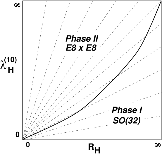
Figure 14: The proposed phase diagram for the $SO(16)\times SO(16)$ interpolating model. For $\lambda_{H}^{(10)}<R_{H}^{2}/(R^{\ast})^{2}$, the theory is in Phase I and flows to the ten-dimensional weakly coupled heterotic supersymmetric $SO(32)$ theory. For $\lambda_{H}^{(10)}>R_{H}^{2}/(R^{\ast})^{2}$, by contrast, the theory is expected to flow to the ten-dimensional strongly coupled supersymmetric $E_{8}\times E_{8}$ string. On the boundary, the theory is stable against passing into Phase I. The dotted lines are contours of constant $T$-dual coupling $\lambda_{H}^{\prime}\equiv\sqrt{\alpha^{\prime}}\lambda_{H}^{(10)}/R_{H}$.

Our results raise a number of interesting questions which will hopefully be addressed in the future.

Perhaps the most obvious question concerns the situation in lower dimensions. This question clearly has important theoretical and phenomenological ramifications. It may seem somewhat disappointing that the ten- and nine-dimensional $SO(16)\times SO(16)$ theories apparently flow to new theories for which supersymmetry is restored. Might there exist stable non-supersymmetric theories in lower dimensions? Our methods can undoubtedly be generalized to lower dimensions, and one would expect the phase structure to be much richer. Indeed, there are certainly many more non-supersymmetric tachyon-free theories in lower dimensions than there are in ten dimensions [32], and hence there are many more candidates.

In fact, one might imagine the following situation. If we assume that the space of supersymmetric string theories in a given dimension forms a closed submanifold within the larger manifold of all self-consistent theories (both supersymmetric and non-supersymmetric), then perhaps this larger manifold consists of subregions with boundaries such that each subregion has an intersection with the submanifold of supersymmetric theories. We can then imagine that whatever strong/weak coupling duality relation is valid on the manifold of supersymmetric theories within a given subregion can be extended throughout the entire subregion. This situation is sketched in Fig. 15.

Figure 15: A proposed generalization of Fig. 14 for string theories in lower dimensions. We show four distinct phases, with the dark line indicating a submanifold of supersymmetric theories. This supersymmetric submanifold runs through the larger manifold like a spine. Within each phase, we conjecture that strong/weak coupling duality can be extended from the supersymmetric spine throughout that phase. The dots indicate the intersections of boundaries between phases, and are conjectured to correspond to stable non-supersymmetric string theories.

In many ways, Fig. 15 can be viewed as a natural generalization of Fig. 14 in that it generalizes the situation that we found in the case of our nine-dimensional interpolating models. Fig. 14 shows, in some sense, a section of the large manifold of self-consistent nine-dimensional theories, and the submanifold of supersymmetric theories corresponds to the top and right axes of Fig. 14. The right axis, clearly, corresponds to the supersymmetric $SO(32)$ theory, and the top axis, because of the infinite coupling and our above conjectures, essentially corresponds to the supersymmetric $E_{8}\times E_{8}$ theory. Fig. 14 indicates how the supersymmetric strong/weak coupling duality relations are extended to the interior of the diagram: points in Phase I flow to the right axis, and points in Phase II flow to the top axis.

Note that there is a critical point at the lower left corner of Fig. 14, corresponding to the ten-dimensional $SO(16)\times SO(16)$ theory at zero coupling. This theory is, of course, completely stable, for it has no interactions and hence no dynamics. In some sense, this stability arises because this point sits on the intersection of boundaries between the two subregions of the theory. It is then natural to imagine that even in lower dimensions, as sketched in Fig. 15, there will be similar manifolds of stable non-supersymmetric tachyon-free theories which are on the intersections of boundaries of the different subregions. Note that while some subregions are expected to have string-theoretic duals, other subregions will have duals that are better described via M-theory.

Another natural question raised by our results concerns whether additional evidence for these non-supersymmetric dualities can be found. In supersymmetric theories, BPS states can be used to provide evidence for duality. Do (stable) tachyon-free string theories contain analogues of BPS states which might be used for the same purpose? In this connection, the notion of “misaligned supersymmetry” [5] might play a crucial role. Indeed, even though these string theories are non-supersymmetric, we have seen in (2.12) that many remarkable constraints continue to govern the resulting string spectrum. It is natural to conjecture that misaligned supersymmetry might be sufficiently powerful to guarantee the BPS-like stability of certain states in the spectra of stable, non-supersymmetric tachyon-free strings.

But perhaps most of all, our results demonstrate that the entire notion of duality may not be as directly tied to supersymmetry as has been thought. This suggests that a reformulation of the ideas and methodologies of strong/weak coupling duality in string theory might be in order.

Acknowledgments

We are happy to thank K.S. Babu, K. Intriligator, J. March-Russell, R. Myers, S. Sethi, F. Wilczek, E. Witten, and especially A. Sagnotti for discussions. This work was supported in part by NSF Grant No.  PHY-95-13835 and DOE Grant No. DE-FG-0290ER40542.

Appendix A

In this Appendix, we give the explicit free-fermionic realizations of the models we have considered in this paper.

A.1 Ten-Dimensional Models

In ten dimensions, are concerned with five different heterotic models: the supersymmetric $SO(32)$ and $E_{8}\times E_{8}$ models, the non-supersymmetric tachyon-free $SO(16)\times SO(16)$ model, and the non-supersymmetric tachyonic $SO(32)$ and $SO(16)\times E_{8}$ models. Using the complex-fermion notation of Ref. [26], these models can be realized as follows. If we begin with the single fermionic boundary condition vector

$${\bf V_{0}}~{}=~{}[\,({\textstyle{1\over 2}})^{4}\,|\,({\textstyle{1\over 2}})^{16}\,]~{},$$ (A.1)

we obtain the non-supersymmetric $SO(32)$ string model. If we now introduce the additional boundary condition vector

$${\bf V_{1}}~{}=~{}[\,(0)^{4}\,|\,({\textstyle{1\over 2}})^{16}\,]~{},$$ (A.2)

we obtain the supersymmetric $SO(32)$ model. In order to produce the remaining models, we introduce a twist corresponding to the additional boundary condition vector

$${\bf V_{2}}~{}=~{}[\,(0)^{4}\,|\,({\textstyle{1\over 2}})^{8}\,(0)^{8}\,]~{}.$$ (A.3)

It then turns out that we can obtain the $E_{8}\times E_{8}$ and $SO(16)\times SO(16)$ models depending on our choice of the corresponding GSO phase. In the free-fermionic notation, such phase choices are given by specifying the values of the independent parameters $k_{20}$ and $k_{21}$. These two parameters reflect the chosen phases of the sectors corresponding to ${\bf V_{2}}$ relative to those corresponding to ${\bf V_{0}}$ and ${\bf V_{1}}$ respectively. If $k_{20}=k_{21}$, the resulting model preserves supersymmetry; if $k_{20}\not=k_{21}$, supersymmetry is broken. We then find that

$$k_{20}=k_{21}~{} \Longrightarrow ~{}{\rm produces}~{}E_{8}\times E_{8}~{}{\rm model}$$

$$k_{20}\not=k_{21}~{} \Longrightarrow ~{}{\rm produces}~{}SO(16)\times SO(16)~{}{\rm model}~{}.$$ (A.4)

The fact that these two models differ merely by a phase in a GSO projection means that the states which are projected out of the spectrum in order to produce the $E_{8}\times E_{8}$ model are kept in the $SO(16)\times SO(16)$ model, and vice versa. Finally, the non-supersymmetric $SO(16)\times E_{8}$ model can be obtained by deleting ${\bf V_{1}}$ from the set of boundary condition vectors. It should be noted that other non-supersymmetric tachyonic heterotic string models can be obtained by adding additional boundary condition vectors to the above list, but these will not be necessary for our purposes.

In general, any two models related through a $\mathchoice{\hbox{\cmss Z\kern-3.99994ptZ}}{\hbox{\cmss Z\kern-3.99994ptZ}}{\lower 0.9pt\hbox{\cmsss Z\kern-2.79996ptZ}}{\lower 1.2pt\hbox{\cmsss Z\kern-2.79996ptZ}}_{2}$ orbifold can be realized in the free-fermionic construction as above through the relative addition or subtraction of a single boundary-condition vector. For example, since deleting the vector ${\bf V_{1}}$ from the supersymmetric $SO(32)$ model produces the non-supersymmetric $SO(32)$ model, these two models are related by a $\mathchoice{\hbox{\cmss Z\kern-3.99994ptZ}}{\hbox{\cmss Z\kern-3.99994ptZ}}{\lower 0.9pt\hbox{\cmsss Z\kern-2.79996ptZ}}{\lower 1.2pt\hbox{\cmsss Z\kern-2.79996ptZ}}_{2}$ orbifold. Thus, simply by examining the above realizations of our ten-dimensional models, we can immediately deduce the pattern of $\mathchoice{\hbox{\cmss Z\kern-3.99994ptZ}}{\hbox{\cmss Z\kern-3.99994ptZ}}{\lower 0.9pt\hbox{\cmsss Z\kern-2.79996ptZ}}{\lower 1.2pt\hbox{\cmsss Z\kern-2.79996ptZ}}_{2}$ orbifold relations indicated in Fig. 4. There is, however, one subtlety, for it would not be immediately apparent from the above fermionic realizations that the $SO(16)\times SO(16)$ string can be realized as an orbifold of the $E_{8}\times E_{8}$ string. However, this orbifold relation does in fact exist, and follows from an alternative fermionic realization of the non-supersymmetric $SO(16)\times SO(16)$ model which starts from the above realization of the $E_{8}\times E_{8}$ model, but which then adds the boundary-condition vector

$${\bf V_{3}}~{}=~{}[\,(0)^{4}\,|\,({\textstyle{1\over 2}})^{4}\,(0)^{4}\,({\textstyle{1\over 2}})^{4}\,(0)^{4}\,]~{}$$ (A.5)

with corresponding phases $k_{30}\not=k_{31}$.

We now give the free-fermionic realizations of the ten-dimensional Type II models. These models can all be realized in the free-fermionic construction through the set of basis vectors:

$${\bf V_{0}} = [\,({\textstyle{1\over 2}})^{4}\,|\,({\textstyle{1\over 2}})^{4}\,]~{}$$

$${\bf V_{1}} = [\,({\textstyle{1\over 2}})^{4}\,|\,(0)^{4}\,]~{}.$$ (A.6)

If we take $k_{00}={1/2}$, we obtain the Type IIA model, whereas if we take $k_{00}=0$, we obtain the Type IIB model. By contrast, if we delete the vector ${\bf V_{1}}$, we then obtain the non-supersymmetric models: with $k_{00}={1/2}$ we obtain the Type 0A model, and with $k_{00}={0}$ we obtain the Type 0B model.

A.2 Nine-Dimensional Models

We now give the explicit free-fermionic construction of the nine-dimensional interpolating models presented in Sect. 3.5. As we discussed in Sect. 3.1, the free-fermionic construction will yield nine-dimensional models formulated at the specific radius $R=\sqrt{2\alpha^{\prime}}$. However, using (3.11) in reverse, it is then a simple matter to extrapolate these models to arbitrary radius. Such radius extrapolations do not affect the self-consistency of these models. It will therefore be sufficient to construct these models at the specific radius $R=\sqrt{2\alpha^{\prime}}$.

To do this, we employ the free-fermionic construction as follows. First, we introduce the following generic set of fermionic boundary condition vectors:

$${\bf V_{0}} = [\,({\textstyle{1\over 2}})^{4}\,({\textstyle{1\over 2}})\,|\,({\textstyle{1\over 2}})^{16}\,({\textstyle{1\over 2}})\,]~{},$$

$${\bf V_{1}} = [\,(0)^{4}\,({\textstyle{1\over 2}})\,|\,({\textstyle{1\over 2}})^{16}\,({\textstyle{1\over 2}})\,]~{},$$

$${\bf V_{2}} = [\,(0)^{4}\,(0)\,|\,({\textstyle{1\over 2}})^{16}\,(0)\,]~{}~{}.$$ (A.7)

Corresponding to these vectors, there then exist three independent relative GSO projection phases which may be chosen. In the free-fermionic notation of Ref. [26], these three phases are given by specifying the values of the three parameters $\{k_{10},k_{20},k_{21}\}$. Since each of these parameters can take two possible values (either 0 or ${\textstyle{1\over 2}}$, corresponding to plus or minus signs in the corresponding GSO projections), this a priori leads to eight possible models. However, there is a great redundancy, and indeed we find that there are only two distinct models (modulo the duality under which the limiting $a\to\infty$ and $a\to 0$ endpoints are exchanged). In general, supersymmetry is preserved if $k_{20}=k_{21}$, and broken otherwise. For $k_{20}=k_{21}$ we obtain the trivial untwisted compactification of the $SO(32)$ string model, while for $k_{20}\not=k_{21}$ we obtain Model A which interpolates between the ten-dimensional supersymmetric and non-supersymmetric $SO(32)$ string models.

In order to obtain the additional interpolating models, we now introduce the additional boundary-condition vector

$${\bf V_{3}}~{}=~{}[\,(0)^{4}\,(0)\,|\,({\textstyle{1\over 2}})^{8}\,(0)^{8}\,(0)\,]{}~{}.$$ (A.8)

Taken together with the previous vectors, this now leaves us with six independent relative GSO projection phases $\{k_{10},k_{20},k_{21},k_{30},k_{31},k_{32}\}$ which may be chosen. In general, supersymmetry is preserved if $k_{20}=k_{21}$ and $k_{30}=k_{31}$, and broken if either of these two conditions is not met. After taking into account various redundancies, this leaves us with six distinct models. The following restrictions on the allowed values of these six parameters will then suffice to specify our string models:

$$\{k_{20}=k_{21},\,k_{30}\not=k_{31},\,k_{30}=k_{32}\} ~{}\Longrightarrow~{} {\rm Model~{}B}~{}$$

$$\{k_{20}\not=k_{21},\,k_{30}=k_{32}\} ~{}\Longrightarrow~{} {\rm Model~{}D}~{}$$

$$\{k_{20}=k_{21},\,k_{30}=k_{31},\,k_{30}\not=k_{32}\} ~{}\Longrightarrow~{} {\rm Model~{}E}~{}$$

$$\{k_{20}\not=k_{21},\,k_{30}\not=k_{32}\} ~{}\Longrightarrow~{} {\rm Model~{}G}~{}$$

$$\{k_{20}=k_{21},\,k_{30}=k_{31},\,k_{30}=k_{32}\} ~{}\Longrightarrow~{} {\rm Model~{}X}~{}$$

$$\{k_{20}=k_{21},\,k_{30}\not=k_{31},\,k_{30}\not=k_{32}\} ~{}\Longrightarrow~{} {\rm Model~{}Y}~{}.$$ (A.9)

Model B is the nine-dimensional model of Sect. 3.5 which interpolates between the supersymmetric $SO(32)$ model and the non-supersymmetric $SO(16)\times SO(16)$ model, while Model D likewise interpolates between the $E_{8}\times E_{8}$ model and the $SO(16)\times E_{8}$ model. These models therefore succeed in interpolating between supersymmetric and non-supersymmetric ten-dimensional models. By contrast, Model E interpolates between the ten-dimensional supersymmetric $SO(32)$ and $E_{8}\times E_{8}$ models, while Model G interpolates between the non-supersymmetric $SO(16)\times SO(16)$ and $SO(16)\times E_{8}$ models. Similarly, Models X and Y are trivial untwisted compactifications of the $E_{8}\times E_{8}$ and $SO(16)\times SO(16)$ strings respectively.

Note that for each of these models, there exists a “dual” model which exchanges the role of radius with inverse radius. Thus, in the dual model, the limiting ten-dimensional models are exchanged. Within the free-fermionic construction, there are two ways of obtaining the dual of a given model. The first is merely to flip the value of $k_{10}$ from 0 to ${\textstyle{1\over 2}}$ or vice versa. The second is to simultaneously flip the values of all of the other independent parameters $\{k_{20},k_{21}\}$ or $\{k_{20},k_{21},k_{30},k_{31},k_{32}\}$. This has the effect of exchanging $a\leftrightarrow 1/(2a)$, which is equivalent to exchanging ${\cal E}_{1/2}\leftrightarrow{\cal O}_{0}$.

Finally, we give the free-fermionic construction of the remaining Model C which interpolates between the supersymmetric $E_{8}\times E_{8}$ model and the non-supersymmetric $SO(16)\times SO(16)$ model. This model can be realized through the introduction of the additional boundary-condition vector

$${\bf V_{4}}~{}=~{}[\,(0)^{4}\,(0)\,|\,({\textstyle{1\over 2}})^{4}\,(0)^{4}\,({\textstyle{1\over 2}})^{4}\,(0)^{4}\,(0)\,]~{}.$$ (A.10)

We then take the GSO projection phase $k_{31}=1/2$, setting $k_{ij}=0$ for all other cases with $i>j$.

We now present our interpolating Type II models. We follow the same procedure as for the heterotic models, and compactify these ten-dimensional Type II models on circles of arbitrary radii. At the fermionic radius $a=1/\sqrt{2}$, the resulting models can be realized via the nine-dimension free-fermionic construction as follows. We begin with the set of basis vectors:

$${\bf V_{0}} = [\,({\textstyle{1\over 2}})^{4}\,({\textstyle{1\over 2}})\,|\,({\textstyle{1\over 2}})^{4}\,({\textstyle{1\over 2}})\,]~{}$$

$${\bf V_{1}} = [\,({\textstyle{1\over 2}})^{4}\,({\textstyle{1\over 2}})\,|\,(0)^{4}\,({\textstyle{1\over 2}})\,]~{}$$

$${\bf V_{2}} = [\,({\textstyle{1\over 2}})^{4}\,(0)\,|\,(0)^{4}\,(0)\,]~{}.$$ (A.11)

We then have four independent GSO-projection phases $\{k_{00},k_{10},k_{20},k_{21}\}$ that must be specified. Generally, $N=2$ supersymmetry is preserved if $k_{20}=k_{21}$ and completely broken to $N=0$ otherwise. We then find that there exist four physically distinct nine-dimensional Type II models, as follows:

$$\{k_{20}\not=k_{21},\,k_{00}+k_{10}+k_{20}\not\in\mathchoice{\hbox{\cmss Z\kern-3.99994ptZ}}{\hbox{\cmss Z\kern-3.99994ptZ}}{\lower 0.9pt\hbox{\cmsss Z\kern-2.79996ptZ}}{\lower 1.2pt\hbox{\cmsss Z\kern-2.79996ptZ}}\} ~{}\Longrightarrow~{} {\rm Model~{}A^{\prime}}~{}$$

$$\{k_{20}\not=k_{21},\,k_{00}+k_{10}+k_{20}\in\mathchoice{\hbox{\cmss Z\kern-3.99994ptZ}}{\hbox{\cmss Z\kern-3.99994ptZ}}{\lower 0.9pt\hbox{\cmsss Z\kern-2.79996ptZ}}{\lower 1.2pt\hbox{\cmsss Z\kern-2.79996ptZ}}\} ~{}\Longrightarrow~{} {\rm Model~{}B^{\prime}}~{}$$

$$\{k_{20}=k_{21},\,k_{00}+k_{10}+k_{20}\in\mathchoice{\hbox{\cmss Z\kern-3.99994ptZ}}{\hbox{\cmss Z\kern-3.99994ptZ}}{\lower 0.9pt\hbox{\cmsss Z\kern-2.79996ptZ}}{\lower 1.2pt\hbox{\cmsss Z\kern-2.79996ptZ}}\} ~{}\Longrightarrow~{} {\rm Model~{}C^{\prime}}~{}$$

$$\{k_{20}=k_{21},\,k_{00}+k_{10}+k_{20}\not\in\mathchoice{\hbox{\cmss Z\kern-3.99994ptZ}}{\hbox{\cmss Z\kern-3.99994ptZ}}{\lower 0.9pt\hbox{\cmsss Z\kern-2.79996ptZ}}{\lower 1.2pt\hbox{\cmsss Z\kern-2.79996ptZ}}\} ~{}\Longrightarrow~{} {\rm Model~{}D^{\prime}}~{}.$$ (A.12)

It turns out that Models ${\rm C}^{\prime}$ and D^′ are trivial untwisted compactifications of the Type IIB and Type IIA models respectively. They therefore interpolate between the Type IIA and IIB theories in opposite directions (i.e., Models C^′ and D^′ are $T$-duals of each other, with both collected together as the single Model C^′ in Fig. 8). By contrast, Models ${\rm A}^{\prime}$ and ${\rm B}^{\prime}$ are non-supersymmetric for general values of the radius, and interpolate between the four ten-dimensional models as indicated in Fig. 8. In each case, the $a\leftrightarrow 1/(2a)$ dual of a given model can be realized by flipping the values of $k_{00}$ and $k_{10}$ from 0 to 1/2 and vice versa.

Finally, we conclude with a brief comment concerning our heterotic Model C. In Ref. [17], a heterotic nine-dimensional string model was constructed which is claimed to interpolate between the ten-dimensional $E_{8}\times E_{8}$ and $SO(16)\times SO(16)$ heterotic models. The authors provide the following partition function as corresponding to their model:

$$Z~{}=~{}Z^{(7)}_{\rm boson}\,\times\,\bigl{\{}~{}\phantom{+} {\cal E}_{0} [{\overline{\chi}}_{S}\,(\chi_{I}^{2}+\chi_{S}^{2})~{}-~{}{\overline{\chi}}_{V}\,(2\,\chi_{I}\chi_{S})]$$

$$+ {\cal E}_{1/2} [{\overline{\chi}}_{I}\,(2\,\chi_{V}\chi_{S})~{}-~{}{\overline{\chi}}_{S}\,(\chi_{V}^{2}+\chi_{S}^{2})]$$

$$+ {\cal O}_{0} [{\overline{\chi}}_{S}\,(2\,\chi_{I}\chi_{S})~{}-~{}{\overline{\chi}}_{V}\,(\chi_{I}^{2}+\chi_{S}^{2})]$$

$$+ {\cal O}_{1/2} [{\overline{\chi}}_{I}\,(\chi_{V}^{2}+\chi_{S}^{2})~{}-~{}{\overline{\chi}}_{S}\,(2\,\chi_{V}\chi_{S})]~{}~{}\bigr{\}}~{}.$$ (A.13)

This expression is indeed modular-invariant, and in the limit $a\to 0$, this does reproduce the $E_{8}\times E_{8}$ partition function. However, in the limit $a\to\infty$, this does not yield the partition function of the $SO(16)\times SO(16)$ model. Indeed, this limit results in an expression which is not a valid partition function.

It is not difficult to show that the function (A.13) cannot correspond to a valid, self-consistent string model. First, we observe that it violates spin-statistics: terms proportional to ${\overline{\chi}}_{S}$ (which come from spacetime fermionic sectors) should always appear in the partition function with minus signs, and terms proportional to ${\overline{\chi}}_{I}$ and ${\overline{\chi}}_{V}$ (spacetime bosonic sectors) should always appear with plus signs. This is not the case for (A.13), in which mixed signs appear. Second, we also observe that this expression is inconsistent with the presence of gravitons. We know that the graviton state, with structure $\psi_{-1/2}^{\mu}|0\rangle_{R}\otimes X_{-1}^{\nu}|0\rangle_{L}$, must always appear in a sector corresponding to a term of the form ${\overline{\chi}}_{V}\chi_{I}^{2}$. However, for general radius, such a term can contain massless states only if it arises in the ${\cal E}_{0}$ sector. Unfortunately, no such term ${\cal E}_{0}{\overline{\chi}}_{V}\chi_{I}^{2}$ arises in (A.13), which signals an inconsistency in this expression. For these two reasons, we doubt the validity of the expression (A.13) as the partition function of a self-consistent string model.

Although the expression (A.13) is clearly invalid as a partition function, this does not necessarily imply that the model constructed in Ref. [17] is invalid. It may simply be that the expression (A.13) does not, in fact, correspond to the model claimed. In any case, our orbifold and free-fermionic constructions of Model C, along with the correct partition function given in (3.22), explicitly demonstrate the existence of a nine-dimensional string model with the desired interpolating properties. Moreover, our general construction procedure demonstrates that in fact a variety of such models exist, as shown in Fig. 5, illustrating that such interpolating models are a completely general feature.

References

- [1] E. Witten, Nucl. Phys. B443 (1995) 85.
- [2] J. Polchinski and E. Witten, Nucl. Phys. B460 (1996) 525.
- [3] P. Hořava and E. Witten, Nucl. Phys. B460 (1996) 506.
- [4] J. Scherk and J.H. Schwarz, Phys. Lett. B82 (1979) 60.
- [5] K.R. Dienes, Nucl. Phys. B429 (1994) 533; hep-th/9409114; hep-th/9505194.
- [6] K.R. Dienes, M. Moshe, and R.C. Myers, Phys. Rev. Lett. 74 (1995) 4767; hep-th/9506001.
- [7] K.R. Dienes, Phys. Rep. 287 (1997) 447 [hep-th/9602045].
-
[8]
I. Antoniadis, C. Bachas, D.C. Lewellen, and T. Tomaras,
Phys. Lett. B207 (1988) 441;
I. Antoniadis, Phys. Lett. B246 (1990) 377;
I. Antoniadis, C. Muñoz, and M. Quirós, Nucl. Phys. B397 (1993) 515;
I. Antoniadis and K. Benakli, Phys. Lett. B326 (1994) 69. -
[9]
S. Ferrara, C. Kounnas, and M. Porrati,
Nucl. Phys. B197 (1987) 135; Phys. Lett. B206 (1988) 25;
Nucl. Phys. B304 (1988) 500;
S. Ferrara, C. Kounnas, M. Porrati, and F. Zwirner, Nucl. Phys. B318 (1989) 75. -
[10]
C. Bachas, hep-th/9503030;
J.G. Russo and A.A. Tseytlin, Nucl. Phys. B461 (1996) 131;
A.A. Tseytlin, hep-th/9510041;
M. Spalinski and H.P. Nilles, Phys. Lett. B392 (1997) 67;
I. Shah and S. Thomas, hep-th/9705182. - [11] H. Kawai, D.C. Lewellen, and S.-H.H. Tye, Phys. Rev. D34 (1986) 3794.
- [12] L. Alvarez-Gaumé, P. Ginsparg, G. Moore, and C. Vafa, Phys. Lett. B171 (1986) 155.
- [13] L.J. Dixon and J.A. Harvey, Nucl. Phys. B274 (1986) 93.
- [14] N. Seiberg and E. Witten, Nucl. Phys. B276 (1986) 272.
- [15] A. Sen, Mod. Phys. Lett. A11 (1996) 1339; Nucl. Phys. B474 (1996) 361.
- [16] R. Rohm, Nucl. Phys. B237 (1984) 553.
- [17] H. Itoyama and T.R. Taylor, Phys. Lett. B186 (1987) 129.
- [18] P. Ginsparg and C. Vafa, Nucl. Phys. B289 (1987) 414.
-
[19]
M. Bianchi and A. Sagnotti, Phys. Lett. B247 (1990) 517;
A. Sagnotti, hep-th/9509080. - [20] O. Bergman and M.R. Gaberdiel, hep-th/9701137.
- [21] S.J. Gates, Jr. and V.G.J. Rodgers, hep-th/9704101.
-
[22]
A. Dabholkar, Phys. Lett. B357 (1995) 307;
C.M. Hull, Phys. Lett. B357 (1995) 545. - [23] J.D. Blum and K.R. Dienes, hep-th/9707148.
- [24] H. Kawai, D.C. Lewellen, and S.-H.H. Tye, Nucl. Phys. B288 (1987) 1.
- [25] I. Antoniadis, C. Bachas, and C. Kounnas, Nucl. Phys. B289 (1987) 87.
- [26] H. Kawai, D.C. Lewellen, J.A. Schwartz, and S.-H.H. Tye, Nucl. Phys. B299 (1988) 431.
- [27] M. Dine, P. Huet, and N. Seiberg, Nucl. Phys. B322 (1989) 301.
- [28] J. Dai, R.G. Leigh, and J. Polchinski, Mod. Phys. Lett. A4 (1989) 2073.
-
[29]
See, e.g.:
A. Sagnotti, in Proceedings of Cargese 1987: Non-Perturbative Quantum Field Theory, eds. G. Mack et al. (Plenum, 1988), p. 521;
P. Hořava, Nucl. Phys. B327 (1989) 461; Phys. Lett. B231 (1989) 251;
J. Dai, R.G. Leigh, and J. Polchinski, Mod. Phys. Lett. A4 (1989) 2073;
G. Pradisi and A. Sagnotti, Phys. Lett. B216 (1989) 59;
M. Bianchi and A. Sagnotti, Nucl. Phys. B361 (1991) 519;
E.G. Gimon and J. Polchinski, Phys. Rev. D54 (1996) 1667. - [30] J. Polchinski and Y. Cai, Nucl. Phys. B296 (1988) 91.
-
[31]
See, e.g.:
G. Moore, Nucl. Phys. B293 (1987) 139; Erratum: ibid. B299 (1988) 847;
T.R. Taylor, Nucl. Phys. B303 (1988) 543;
J. Balog and M.P. Tuite, Nucl. Phys. B319 (1989) 387;
K.R. Dienes, Phys. Rev. D42 (1990) 2004;
T. Gannon and C.S. Lam, Phys. Rev. D46 (1992) 1710. - [32] K.R. Dienes, Phys. Rev. Lett. 65 (1990) 1979.
- [33] P. Ginsparg, Phys. Rev. D35 (1987) 648.
- [34] J.D. Blum and K.R. Dienes, to appear.
- [35] M. Dine and N. Seiberg, Phys. Rev. Lett. 55 (1985) 366; Phys. Lett. B162 (1985) 299.
- [36] V.P. Nair, A. Shapere, A. Strominger, and F. Wilczek, Nucl. Phys. B287 (1987) 402.
- [37] P. Hořava, Phys. Rev. D54 (1996) 7561.