IASSNS-HEP-97/67

hep-th/9707148

July 1997

Duality without Supersymmetry:
The Case of the $SO(16)\times SO(16)$ String
Julie D. Blum  and  Keith R. Dienes
School of Natural Sciences, Institute for Advanced Study
Olden Lane, Princeton, N.J.  08540  USA

We extend strong/weak coupling duality to string theories without spacetime supersymmetry, and focus on the case of the unique ten-dimensional, nonsupersymmetric, tachyon-free $SO(16)\times SO(16)$ heterotic string. We construct a tachyon-free heterotic string model that interpolates smoothly between this string and the ten-dimensional supersymmetric $SO(32)$ heterotic string, and we construct a dual for this interpolating model. We find that the perturbative massless states of our dual theories precisely match within a certain range of the interpolation. Further evidence for this proposed duality comes from a calculation of the one-loop cosmological constant in both theories, as well as the presence of a soliton in the dual theory. This is therefore the first known duality relation between nonsupersymmetric tachyon-free string theories. Using this duality, we then investigate the perturbative and nonperturbative stability of the $SO(16)\times SO(16)$ string, and present a conjecture concerning its ultimate fate.

1 Introduction

Much has been learned about the nonperturbative properties of superstring theories by mapping these theories at strong coupling into other theories at weak coupling. The constraints of supersymmetry provide much of the structure of these duality relations, but one would like to understand whether duality might be a more general property of string theory which holds even without supersymmetry. One might then begin to understand the nonperturbative properties of nonsupersymmetric theories as well.

As a step in this direction, we will study nonsupersymmetric duality by smoothly connecting nonsupersymmetric ten-dimensional theories to supersymmetric ten-dimensional theories. Such connections can be achieved in nine dimensions through interpolating models. Dimensional reduction as a means of breaking supersymmetry in string theory was originally proposed in Ref. [1], and interpolating models of this sort have been discussed in Refs. [1, 2, 3].

As our focus, we shall consider the case of the $SO(16)\times SO(16)$ string [4]. This is the unique, tachyon-free, nonsupersymmetric heterotic string theory in ten dimensions, and it can therefore be viewed as the nonsupersymmetric counterpart of the supersymmetric $SO(32)$ and $E_{8}\times E_{8}$ strings. The absence of tachyons in this theory is very important, implying that its one-loop cosmological constant is finite. This makes a stability analysis possible. The absence of tachyons also guarantees a number of other remarkable properties, such as the existence of a hidden “misaligned supersymmetry” [5] in the string spectrum.

As a means of investigating strong/weak duality relations for the $SO(16)\times SO(16)$ string, we will use the interpolation idea and begin by constructing a heterotic interpolating model that smoothly connects the nonsupersymmetric $SO(16)\times SO(16)$ string to the supersymmetric $SO(32)$ string. Our model will be a twisted compactification of the supersymmetric $SO(32)$ heterotic string on a circle of radius $R_{H}$. Our twists will be chosen in such a way that the theory reproduces the ten-dimensional supersymmetric $SO(32)$ theory as $R_{H}\to\infty$, but is related by $T$-duality to the ten-dimensional nonsupersymmetric $SO(16)\times SO(16)$ string as $R_{H}\to 0$.

Our next step will be to construct the strong-coupling dual of this interpolating model. The fact that this interpolating model continuously connects the $SO(16)\times SO(16)$ theory to the supersymmetric $SO(32)$ theory suggests that the dual of our interpolating model is an open-string model. We therefore study the possible interpolations of open-string models. We find that we are able to construct a corresponding nine-dimensional open-string model which interpolates between the ten-dimensional $SO(32)$ Type I theory as $R_{I}\to\infty$, and a ten-dimensional nonsupersymmetric, tachyonic open-string theory at $R_{I}=0$. It might initially seem that the appearance of tachyons in our open-string interpolating model might ruin our attempted duality relation, or at the very least render it meaningless. However, there exists a critical radius $R^{\ast}$ above which our open-string interpolating model is completely free of tachyons, and it is in precisely this range that we find evidence for an exact duality relation. Specifically, we find that for $R_{I}>R^{\ast}$, the perturbative massless spectrum of the open-string interpolating model agrees exactly with that of our corresponding heterotic interpolating model. Furthermore, our open-string model contains a soliton which (modulo several assumptions) behaves as a fundamental $SO(16)\times SO(16)$ nonsupersymmetric heterotic string when the ten-dimensional Type I coupling $\lambda^{(10)}_{I}$ is large, or equivalently when the ten-dimensional heterotic coupling $\lambda^{(10)}_{H}=1/\lambda^{(10)}_{I}$ is small. Thus, if our interpretation is correct, this duality between our heterotic and open-string interpolating models would be the first known example of a strong/weak coupling duality relation between nonsupersymmetric, tachyon-free string theories.

Our results for this model — as well as similar results for several other nonsupersymmetric interpolating models — will be given in great detail in Ref. [8]. Here we shall merely outline and summarize our results for the $SO(16)\times SO(16)$ case. In Sect. 2, we describe our heterotic interpolating model and discuss its one-loop cosmological constant. Then, in Sect. 3, we construct our proposed dual model, and discuss its one-loop cosmological constant as well. In Sect. 4, we examine the soliton of our dual open-string theory, and in Sect. 5 we make use of our duality relation in order to analyze the stability of these models and make a conjecture about the behavior of the $SO(16)\times SO(16)$ nonsupersymmetric heterotic string. We find that we are able to propose a phase diagram that describes the behavior of this string as a function of its coupling and radius. Finally, Sect. 6 contains our conclusions.

2 The $SO(16)\times SO(16)$ Heterotic Interpolating Model

Our goal in this section is to construct a model which interpolates between the ten-dimensional $SO(32)$ supersymmetric heterotic string and the ten-dimensional $SO(16)\times SO(16)$ nonsupersymmetric heterotic string. To do this, we compactify the $SO(32)$ theory on a circle of radius $R_{H}$ and orbifold by a $\mathchoice{\hbox{\cmss Z\kern-3.99994ptZ}}{\hbox{\cmss Z\kern-3.99994ptZ}}{\lower 0.9pt\hbox{\cmsss Z\kern-2.79996ptZ}}{\lower 1.2pt\hbox{\cmsss Z\kern-2.79996ptZ}}_{2}$ element $Q^{\prime}_{H}\equiv{\cal T}Q_{H}$ defined as follows. The operator $\cal T$ is a translation of the coordinate $x_{1}$ of the circle by half of the circumference of the circle:

$${{\cal T}:\hskip 5.69046ptx_{1}\rightarrow x_{1}+\pi R_{H}~{}.}$$ (2.1)

The operator $Q_{H}$ is the generator of the orbifold that produces the ten-dimensional nonsupersymmetric $SO(16)\times SO(16)$ theory from the ten-dimensional supersymmetric $SO(32)$ theory. Note that if we decompose the representations of the original gauge group $SO(32)$ into those of $SO(16)\times SO(16)$, then $Q_{H}$ can be written as $(-1)^{F}{\cal R}$ where $F$ is the spacetime fermion number and where ${\cal R}$ acts with a minus sign on both of the spinors of one of the $SO(16)$ factors, and with a minus sign on the vector and one of the spinor representations of the other factor.

Projection by the half-rotation operator ${\cal T}$ by itself has the effect of halving the radius of the circle, for odd momentum states on the circle are not invariant under ${\cal T}$ and are projected out of the spectrum. However, at infinite radius, the odd momentum states are degenerate with the even momentum states. This causes ${\cal T}$ to act as zero in this case, which merely amounts to a rescaling of the effective volume normalization of the $SO(32)$ partition function. We thus recover the ten-dimensional supersymmetric $SO(32)$ theory. At zero radius, all momentum states are infinitely massive so the orbifold action reduces to $Q_{H}$. This gives us the $SO(16)\times SO(16)$ theory at $R_{H}=0$, and by $T$-duality this theory is equivalent to the uncompactified $SO(16)\times SO(16)$ theory in ten dimensions. Spacetime supersymmetry is broken for all finite radii, and there are no tachyons in this model for any radius. Note also that the $SO(32)$ gauge symmetry is restored only at the infinite-radius endpoint, and there are no enhanced gauge symmetries at any finite radius. For generic radii in the range $0<R_{H}<\infty$, the massless states of this model consist of the graviton, antisymmetric tensor, dilaton, two $U(1)$ vectors, vectors in the adjoint representation of $SO(16)\times SO(16)$, and a spinor in the $({\bf{16}},{\bf{16}})$ representation. At the discrete radius $R_{H}=\sqrt{2\alpha^{\prime}}$ there are also two massless scalars in the $({\bf{1}},{\bf{128}})\oplus({\bf{128}},{\bf{1}})$ representation, and at the discrete radius $R_{H}=\sqrt{\alpha^{\prime}}$ there are two massless spinors that are singlets under $SO(16)\times SO(16)$. As $R_{H}\to 0$, a massive opposite-chirality spinor in the $({\bf{1}},{\bf{128}})\oplus({\bf{128}},{\bf{1}})$ representation becomes massless, and the $U(1)$ gauge bosons disappear.

The one-loop vacuum amplitude or cosmological constant of this model can be calculated, and the results are shown in Fig. 1. Note that we have taken

$$\Lambda^{(9)}(R_{H})~{}\equiv~{}-\,{\textstyle{1\over 2}}\,{\cal M}^{9}\,\int_{\cal F}{d^{2}\tau\over({\rm Im}\,\tau)^{2}}\,Z(\tau,R_{H})$$ (2.2)

where $Z(\tau,R_{H})$ is the radius-dependent partition function of the interpolating model and where ${\cal M}\equiv(4\pi^{2}\alpha^{\prime})^{-1/2}$. We can also define

$$\tilde{\Lambda}(R_{H})~{}\equiv~{}{\cal M}\,{R_{H}\over\sqrt{\alpha^{\prime}}}\,\Lambda^{(9)}(R_{H})~{}.$$ (2.3)

Thus $\lim_{R_{H}\to 0}\tilde{\Lambda}(R_{H})$ is finite, and gives the ten-dimensional cosmological constant of the $SO(16)\times SO(16)$ string.

     

Figure 1: The one-loop cosmological constants $\Lambda^{(9)}$ (left plot) and $\tilde{\Lambda}$ (right plot) as functions of the radius $R_{H}$ of the compactified dimension, in units of ${\textstyle{1\over 2}}{\cal M}^{9}$ and ${\textstyle{1\over 2}}{\cal M}^{10}$ respectively. This model reproduces the supersymmetric $SO(32)$ heterotic string as $R_{H}\to\infty$ and the nonsupersymmetric $SO(16)\times SO(16)$ heterotic string as $R_{H}\to 0$.

Several observations are worth mentioning. The nine-dimensional cosmological constant $\Lambda^{(9)}$ is positive and finite for all finite, nonzero radii. At infinite radius, the cosmological constant vanishes, and there is a critical point with zero slope. The slope of the curve is negative for all finite positive radii.

3 The Dual Interpolating Model

We now construct our proposed dual for the $SO(16)\times SO(16)$ heterotic interpolating model of Sect. 2.

Our method for constructing open-string interpolating models will be as follows. We take the point of view that a given open-string model is consistent if it can be realized as the orientifold [9, 6] of a Type II model, and if it satisfies tadpole anomaly-cancellation constraints. We therefore begin by examining Type II interpolating models, and in particular we construct a nine-dimensional interpolating model that connects the supersymmetric Type IIB theory at infinite radius to the nonsupersymmetric so-called Type 0B theory [10] at zero radius. At zero radius, the nonsupersymmetric Type 0B endpoint is equivalent by $T$-duality to the so-called Type 0A theory [10]. This Type II interpolating model is similar to that considered in Ref. [11]. In particular, it can be realized by compactifying the Type IIB theory on a circle of radius $R_{I}$, and then orbifolding by the action $g={\cal T}(-1)^{F}$. Here ${\cal T}$ is again the operator given in Eq. (2.1), and $F\equiv F_{L}+F_{R}$ is the total Type II spacetime fermion number. Because of the factor $(-1)^{F}$ within $g$, orbifolding by $g$ breaks supersymmetry for all radii $R_{I}<\infty$.

Given this Type II interpolating model, we then construct its corresponding open-string orientifold. We take our orientifold generator to be $\Omega$, the worldsheet parity operator. Thus, putting our entire construction together, we see that our open-string interpolating model is a $\mathchoice{\hbox{\cmss Z\kern-3.99994ptZ}}{\hbox{\cmss Z\kern-3.99994ptZ}}{\lower 0.9pt\hbox{\cmsss Z\kern-2.79996ptZ}}{\lower 1.2pt\hbox{\cmsss Z\kern-2.79996ptZ}}_{2}\times\mathchoice{\hbox{\cmss Z\kern-3.99994ptZ}}{\hbox{\cmss Z\kern-3.99994ptZ}}{\lower 0.9pt\hbox{\cmsss Z\kern-2.79996ptZ}}{\lower 1.2pt\hbox{\cmsss Z\kern-2.79996ptZ}}_{2}$ orientifold of the supersymmetric Type IIB theory compactified on a circle of radius $R_{I}$. The first $\mathchoice{\hbox{\cmss Z\kern-3.99994ptZ}}{\hbox{\cmss Z\kern-3.99994ptZ}}{\lower 0.9pt\hbox{\cmsss Z\kern-2.79996ptZ}}{\lower 1.2pt\hbox{\cmsss Z\kern-2.79996ptZ}}_{2}$ factor corresponds to the worldsheet parity operator $\Omega$, and the second to the orbifold operator $g$. Because these two operators commute, we can consider our interpolating open-string model either as an orientifold of the Type II interpolation, or as an orbifold of the $SO(32)$ Type I theory. As $R_{I}\to\infty$, this open-string model smoothly reproduces the supersymmetric $SO(32)$ Type I theory. Further details concerning the construction of this model can be found in Ref. [8].

The one-loop amplitudes for our orientifold model can be calculated for the torus, Klein bottle, cylinder, and Möbius strip. As is usual for orientifolds, for each of the elements $\Omega$ and $g$ we must specify an action on the Chan-Paton factors of the open-string sectors. Remarkably, it then turns out [8] that both the NS-NS and Ramond-Ramond massless tadpole divergences will be cancelled for $R_{I}>0$ if the gauge group is $SO(16)\times SO(16)$. This choice also avoids introducing open-string tachyonic divergences.

This open-string interpolating model contains a critical radius $R^{\ast}\equiv 2\sqrt{2\alpha^{\prime}}$. For radii $R_{I}$ in the range $R^{\ast}<R_{I}<\infty$, the massless spectrum of our model consists of the graviton, antisymmetric tensor, dilaton, two $U(1)$ vectors, vectors in the adjoint of $SO(16)\times SO(16)$, and a spinor in the $({\bf{16}},{\bf{16}})$ representation. There are no tachyons in either the closed-string or open-string sectors. The massless spectrum of this model therefore agrees precisely with that of its heterotic dual in this range. We emphasize that a perturbative comparison of the spectra of these dual theories is only possible in the nontachyonic range of the interpolation with $R_{I}>R^{\ast}$.

At $R_{I}=R^{\ast}=2\sqrt{2\alpha^{\prime}}$, two additional massless closed-string states appear, and these become tachyonic for $R_{I}<R^{\ast}$. In fact, an infinite number of closed-string tachyons appear at discrete radii in the range $R_{I}<R^{\ast}$. Nevertheless, all tadpole anomalies continue to cancel for $R_{I}>0$.

Figure 2: The total one-loop cosmological constant $\tilde{\Lambda}$ for our open-string interpolating model, plotted in units of ${\textstyle{1\over 2}}{\cal M}^{10}$, as a function of the radius $R_{I}$ of the compactified dimension. Also shown (dashed lines) are the separate torus and Möbius-strip contributions; note that the Klein-bottle and cylinder contributions vanish. This open-string model reproduces the supersymmetric $SO(32)$ Type I string as $R_{I}\to\infty$, and has gauge group $SO(16)\times SO(16)$ for all finite radii. The torus amplitude develops a divergence below $R^{\ast}/\sqrt{\alpha^{\prime}}\equiv 2\sqrt{2}\approx 2.83$, which reflects the appearance of a tachyon in the torus amplitude below this radius. All other contributions are tachyon-free for all radii.

Just as for our heterotic interpolating model, we can calculate the one-loop cosmological constant for our open-string model. A priori, this receives four contributions, one each from the torus, Klein bottle, cylinder, and Möbius strip. However, for this model, the Klein bottle and cylinder contributions vanish exactly. This occurs because the Klein bottle is immune to supersymmetry breaking for $R_{I}>0$, and because we have chosen the gauge symmetry to be $SO(16)\times SO(16)$. Thus only the torus and Möbius contributions remain, and these contributions are shown in Fig. 2. Note that for this figure, we have used the alternate definition

$$\tilde{\Lambda}(R_{I})~{}\equiv~{}{\cal M}\,{\sqrt{\alpha^{\prime}}\over R_{I}}\,\Lambda^{(9)}(R_{I})~{}$$ (3.1)

where $\Lambda^{(9)}$ is defined as the (appropriately weighted) sum of the modular integrals of the torus and Möbius strip partition functions. This definition ensures that $\tilde{\Lambda}(R_{I})$ formally reproduces the Type I $SO(32)$ cosmological constant as $R_{I}\to\infty$.

It is clear from this figure that the torus contribution to the cosmological constant is strictly negative. Fortunately, the Möbius contribution more than cancels the torus contribution, and produces a net positive cosmological constant for all radii $R^{\ast}<R_{I}<\infty$. It turns out that $SO(16)\times SO(16)$ is the unique gauge symmetry that can be chosen in our open-string model for which the net cosmological constant is positive rather than negative for $R_{I}>R^{\ast}$. Moreover, the slope of the curve is strictly negative in this range, and vanishes at infinity.

It is interesting that the inclusion of open-string sectors in tachyon-free theories can provide competing contributions to the cosmological constant. This suggests that it might be possible to cancel the contributions of open-string sectors against those of closed-string sectors in order to provide a new mechanism for cancelling the cosmological constant in open-string theories.

As we have remarked above, closed-string tachyons appear in this model at $R_{I}<R^{\ast}$. There is therefore a discontinuity in the cosmological constant at the critical point $R_{I}=R^{\ast}$, suggestive of a phase transition in our open-string theory. We shall explore this idea further in Sect. 5.

4 The Soliton

Our open-string model contains a solitonic object or D1-brane. Solitons of the $SO(32)$ Type I theory corresponding to $SO(32)$ heterotic strings were found as classical solutions in Ref. [12], and were constructed from a collective-coordinate expansion on the D1-brane in Ref. [13]. In this section, we will construct the soliton of our model by projecting the worldsheet fields of the $SO(32)$ soliton by the orbifold element $g$. This procedure involves numerous subtleties, and a fuller discussion can be found in Ref. [8]. Here we summarize only the salient features.

The tension of the soliton is $T_{S}\sim T_{F}/\lambda_{I}^{(10)}$ where $T_{F}=1/2\pi\alpha^{\prime}$ is the fundamental string tension and where $\lambda_{I}^{(10)}$ is the ten-dimensional Type I coupling. If we were to choose the soliton to lie along any direction orthogonal to the compact direction, the soliton would be very heavy for all perturbative values of the coupling and would not behave as a fundamental object. Thus, we shall choose the soliton to lie along the compact $x_{1}$ direction because this choice allows states of the soliton to become nearly massless at perturbative values of the couplings for sufficiently small $R_{I}$. Note, though, that our soliton is not expected to behave fundamentally in the range of the interpolation where a perturbative analysis is valid.

In quantizing the fields on the soliton, we find that the quantized zero-mode momentum of Type I bosons in the $x_{1}$ direction becomes the quantized oscillator moding of the worldsheet fields on the soliton. Moreover, the Type I theory provides a restriction on the left- and right-moving momenta of the form $p_{1}^{L}=p_{1}^{R}$, and this restriction becomes the worldsheet restriction $L_{0}=\overline{L_{0}}$ on the left- and right-moving Virasoro generators on the soliton.

We will project by the $\mathchoice{\hbox{\cmss Z\kern-3.99994ptZ}}{\hbox{\cmss Z\kern-3.99994ptZ}}{\lower 0.9pt\hbox{\cmsss Z\kern-2.79996ptZ}}{\lower 1.2pt\hbox{\cmsss Z\kern-2.79996ptZ}}_{2}$ element ${\cal Y}={\cal T}(-1)^{F}\gamma_{g}$ where $\gamma_{g}$ is the Type I Wilson line that breaks $SO(32)$ to $SO(16)\times SO(16)$. It turns out that the action of $(-1)^{F}\gamma_{g}$ on the worldsheet fields of the $SO(32)$ soliton exactly corresponds to $Q_{H}$. Since $(-1)^{F}\gamma_{g}$ does not act on the Type I spacetime, the spacetime action of ${\cal Y}$ is solely due to $\cal T$, and effectively halves the radius of the circle. All worldsheet bosons of the soliton will thus be restricted to integral moding such that these fields are periodic on the half-radius circle.

Before the projection, the right-movers along $x_{1}$ consist of eight transverse spatial bosonic fields $X^{i}$, $i=1,...,8$, and a Green-Schwarz fermion $S^{a}$, $a=1,...,8$, of definite chirality. The left-movers consist of eight transverse spatial bosonic fields $X^{i}$ and 32 worldsheet fermions $\psi^{A}$, $A=1,...,32$. There is also a GSO projection acting on the left-moving fermions. It is convenient in our analysis to separate the fields on the half-radius circle into two groups. The “Class A” sectors will be those for which all fields have the usual modings on the half-radius circle (such that the fields are periodic on the half-radius circle), while the “Class B” sectors will be those in which some fields may be antiperiodic on the half-radius circle (provided they are consistent with the symmetries preserved by the orbifold). This describes the Ramond sector of the soliton, and just as for the supersymmetric $SO(32)$ soliton, we will assume that a Neveu-Schwarz sector arises nonperturbatively.

We emphasize that it is the projection onto the half-radius circle that gives rise to the Class B sectors. Specifically, we have not added the Class B sectors by hand — they instead appear naturally when the original fields on the circle of radius $R_{I}$ are decomposed into fields on the circle of half-radius $R_{I}/2$. This passing from the original radius to the half-radius naturally generates the unexpected modings. Note that because of their nontraditional modings, all Class B sectors would be ordinarily be projected out of the spectrum by the operator ${\cal T}$ alone.

We can summarize the resulting sectors in the following tables where the identity, vector, spinor, and conjugate-spinor representations of the right-moving transverse Lorentz group $SO(8)$ and the two left-moving $SO(16)$ gauge factors are labelled in an obvious way. For each, we have also indicated the corresponding eigenvalue under ${\cal Y}$. The Class A sectors are:

right-movers left-movers

Ramond NS

$${\cal Y}$$ sector sector sector

(4.1)

and the Class B sectors are:

right-movers left-movers

Ramond NS

$${\cal Y}$$ sector sector sector

(4.2)

The final step, then, is to join these left- and right-moving sectors together. In order to do this, we make the following assumptions. First, as discussed above, we impose the requirement that $L_{0}=\overline{L_{0}}$. Second, we require that the exchange symmetry of the two $SO(16)$ gauge factors be preserved. Third, we require that all left/right combinations be invariant under ${\cal Y}$. And finally, we demand that the Class A and Class B not be permitted to mix when joining left- and right-moving sectors. If we impose all four of these restrictions simultaneously, we obtain precisely the sectors that comprise the nonsupersymmetric $SO(16)\times SO(16)$ heterotic string:

$${\rm Class~{}A:} ~{}~{}~{}V_{8}\,I_{16}^{(1)}I_{16}^{(2)}~{},~{}~{}V_{8}\,S_{16}^{(1)}S_{16}^{(2)}~{},~{}~{}S_{8}\,V_{16}^{(1)}V_{16}^{(2)}~{},~{}~{}S_{8}\,C_{16}^{(1)}C_{16}^{(2)}$$

$${\rm Class~{}B:} ~{}~{}~{}I_{8}\,V_{16}^{(1)}C_{16}^{(2)}~{},~{}~{}I_{8}\,C_{16}^{(1)}V_{16}^{(2)}~{},~{}~{}C_{8}\,I_{16}^{(1)}S_{16}^{(2)}~{},~{}~{}C_{8}\,S_{16}^{(1)}I_{16}^{(2)}~{}.$$ (4.3)

It is apparent from this correspondence between our soliton and the $SO(16)\times SO(16)$ nonsupersymmetric string that the Class A sectors correspond to the untwisted sectors of the heterotic theory while the Class B sectors correspond to the twisted sectors of the heterotic theory. We find it quite miraculous that these twisted sectors, which are required by modular invariance on the heterotic side, automatically appear on the Type I side via the above simple decomposition and projection by ${\cal Y}$. This indicates that the D1-brane soliton somehow manages to reconstruct modular invariance, even without supersymmetry. This issue will be discussed more fully in Ref. [8].

Note that our third restriction permits combinations of left- and right-moving sectors that are not separately invariant under ${\cal Y}$. This can be interpreted as an interaction between such sectors, and makes sense at strong coupling. Likewise, our fourth restriction is essentially a nonperturbative selection rule. While both of these restrictions are plausible at strong coupling, they are somewhat implausible at weak coupling. However, it is very interesting to note that if we remove the fourth restriction entirely and enforce a strict projection by ${\cal Y}$ on the left- and right-moving sectors separately, then we instead obtain the massless sectors of the $E_{8}\times E_{8}$ supersymmetric heterotic string:

$$~{}~{}~{}V_{8}\,I_{16}^{(1)}I_{16}^{(2)}~{},~{}~{}V_{8}\,S_{16}^{(1)}S_{16}^{(2)}~{},~{}~{}V_{8}\,S_{16}^{(1)}I_{16}^{(2)}~{},~{}~{}V_{8}\,I_{16}^{(1)}S_{16}^{(2)}~{},~{}~{}$$

$$~{}~{}~{}C_{8}\,I_{16}^{(1)}I_{16}^{(2)}~{},~{}~{}C_{8}\,S_{16}^{(1)}S_{16}^{(2)}~{},~{}~{}C_{8}\,S_{16}^{(1)}I_{16}^{(2)}~{},~{}~{}C_{8}\,I_{16}^{(1)}S_{16}^{(2)}~{},~{}~{}$$

$$~{}~{}~{}I_{8}\,V_{16}^{(1)}C_{16}^{(2)}~{},~{}~{}I_{8}\,C_{16}^{(1)}V_{16}^{(2)}~{}.~{}~{}$$ (4.4)

Indeed, the only extra sectors in the above list that are not found in the $E_{8}\times E_{8}$ string are those in the last line above. These are purely massive, however, and become infinitely massive as $R_{I}\rightarrow 0$. They can therefore be expected to decouple completely.

We thus conclude that at strong coupling, the soliton is expected to behave as an $SO(16)\times SO(16)$ heterotic string, whereas at weak coupling, the massless worldsheet fields on the soliton are those of an $E_{8}\times E_{8}$ heterotic string.

5 The Fate of the $SO(16)\times SO(16)$ String:
Analysis and Conjecture

Using our candidate open-string dual, we now proceed to address questions of stability.

At the supersymmetric $R_{I}=R_{H}=\infty$ endpoints, the relation

$${\lambda_{I}^{(10)}={1\over\lambda_{H}^{(10)}}}$$ (5.1)

is expected to be valid where $\lambda_{H}^{(10)}$ is the ten-dimensional heterotic coupling. Since there is no perturbative discontinuity in our orientifold for $R_{I}>R^{\ast}$, we will assume that this relation continues to be valid there.

We will need to distinguish the tachyon-free Phase I where $R_{I}>R^{\ast}$ and $\lambda_{H}^{(10)}<R_{H}^{2}/{(R^{\ast})}^{2}$ from Phase II where $R_{I}<R^{\ast}$ and $\lambda_{H}^{(10)}>R_{H}^{2}/{(R^{\ast})}^{2}$. For $R_{I}>R^{\ast}$, the massless states in the two theories exactly match. The nine-dimensional heterotic coupling is $\lambda_{H}^{(9)}=\lambda_{H}^{(10)}/\sqrt{R_{H}}$ and similarly for $\lambda_{I}^{(9)}$. We thus have the following bounds in Phase I:

$${{{(R^{\ast})}^{2}\over R_{H}^{5/2}}~{}<~{}\lambda_{I}^{(9)}~{}<~{}{1\over{(R^{\ast})}^{1/2}\lambda_{H}^{(10)}}}$$ (5.2)

and

$$\lambda_{H}^{(9)}~{}<~{}{R_{H}^{3/2}\over(R^{\ast})^{2}}~{}.$$ (5.3)

If we fix $\lambda_{H}^{(10)}$ at a sufficiently small value, our calculation of the heterotic cosmological constant $\Lambda^{(9)}$, together with the arguments of Refs. [14, 15], suggest that for $R_{H}>0$ the heterotic theory should flow in the direction of increasing $R_{H}$ (or decreasing $\lambda_{H}^{(9)}$) towards the supersymmetric $SO(32)$ endpoint. There is a subtlety in the analysis as $R_{H}\rightarrow\infty$ [15], but this conclusion remains valid [8]. The soliton should behave fundamentally in this phase of the theory, but is clearly unstable. For $\lambda_{H}^{(10)}$ large enough but still in Phase I, our perturbative calculation of the cosmological constant of the dual theory indicates that the dual theory also flows to the supersymmetric $SO(32)$ endpoint. Note that the $R_{H}=0$ endpoint is not in the Phase I region for any value of the coupling $\lambda_{H}^{(10)}$.

Since there is a phase transition connecting Phase I to Phase II, we expect a different behavior in Phase II. We cannot analyze the dual theory in Phase II because of the presence of tachyons, but we might try to relate the heterotic theory to M-theory. This makes sense since the length $\rho$ of the eleventh dimension, defined in M-theory units as

$$\rho~{}\equiv~{}{{[\lambda_{H}^{(10)}]}^{2/3}\over R_{H}^{2/3}}~{},$$ (5.4)

satisfies

$$\rho~{}>~{}{[\lambda_{H}^{(10)}]^{1/3}\over(R^{\ast})^{2/3}}~{}.$$ (5.5)

Thus $\rho$ is bounded from below. The low-energy analysis of Ref. [16] seems to indicate that there are no stable solutions of M-theory on a line segment breaking supersymmetry in nine dimensions. This, combined with the fact that there is a phase transition separating Phase I from Phase II, leads to several conjectures for the behavior of our model. Since it turns out [8] that both the ten-dimensional $SO(32)$ and $E_{8}\times E_{8}$ supersymmetric heterotic strings are continuously connected via interpolating models to the $SO(16)\times SO(16)$ theory, one conjecture is that the theory flows to a strongly coupled $E_{8}\times E_{8}$ theory, or equivalently to M-theory on $S^{1}/{\mathchoice{\hbox{\cmss Z\kern-3.99994ptZ}}{\hbox{\cmss Z\kern-3.99994ptZ}}{\lower 0.9pt\hbox{\cmsss Z\kern-2.79996ptZ}}{\lower 1.2pt\hbox{\cmsss Z\kern-2.79996ptZ}}_{2}}$. From what we have said about the expected behavior of the soliton at weak coupling, it is plausible that there is a phase transition at $R_{H}=0$ such that when the $T$-dual ten-dimensional theory has nonzero coupling $\lambda_{H}^{\prime}\equiv\lambda_{H}^{(10)}\sqrt{\alpha^{\prime}}/R_{H}$, a fundamental $SO(16)\times SO(16)$ string in ten dimensions behaves as an $E_{8}\times E_{8}$ string. The subtlety discussed in Ref. [15] further indicates that the boundary of the Phase I region at $\lambda_{H}^{(10)}=R_{H}^{2}/{(R^{\ast})}^{2}$ is stable against falling into Phase I, at least for small $R_{H}$. Moreover, by continuity arguments, we expect that this result can be extended for all $R_{H}$. However, the above argument does not apply in Phase II, and thus we have the interesting possibility that this theory might spontaneously compactify sufficiently many additional dimensions so that it could be stabilized, for example, via a gluino condensate as in the model of Ref. [16].

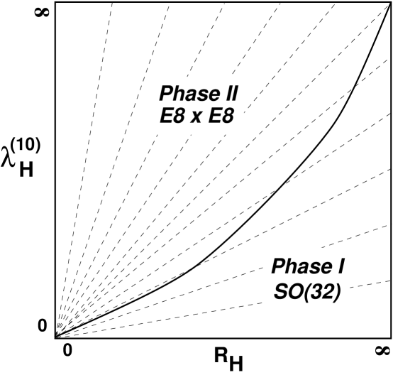
Figure 3: The proposed phase diagram for the $SO(16)\times SO(16)$ interpolating model. For $\lambda_{H}^{(10)}<R_{H}^{2}/(R^{\ast})^{2}$, the theory is in Phase I and flows to the ten-dimensional weakly coupled heterotic supersymmetric $SO(32)$ theory. For $\lambda_{H}^{(10)}>R_{H}^{2}/(R^{\ast})^{2}$, by contrast, the theory is expected to flow to the ten-dimensional strongly coupled supersymmetric $E_{8}\times E_{8}$ string. On the boundary, the theory is stable against passing into Phase I. The dotted lines are contours of constant $T$-dual coupling $\lambda_{H}^{\prime}\equiv\sqrt{\alpha^{\prime}}\lambda_{H}^{(10)}/R_{H}$.

The results of our stability analysis can thus be summarized as in Fig. 3, which shows our proposed phase diagram for the $SO(16)\times SO(16)$ interpolating model.

6 Conclusions

We have constructed an exact strong/weak coupling dual for a nonsupersymmetric, tachyon-free, heterotic theory that interpolates between the ten-dimensional supersymmetric $SO(32)$ theory and the ten-dimensional nonsupersymmetric $SO(16)\times SO(16)$ theory. Our duality relation is valid within a range of our interpolating parameter corresponding to the tachyon-free phase of the dual interpolating theory. In this tachyon-free phase, the two dual theories behave identically, have the same massless states, and flow to the supersymmetric $SO(32)$ theory. Furthermore, the dual theory contains a soliton that should behave as a fundamental $SO(16)\times SO(16)$ string at sufficiently strong dual coupling. We have conjectured that outside of this range, the strongly coupled heterotic theory — including the ten dimensional $SO(16)\times SO(16)$ theory itself — flows to the supersymmetric strongly coupled $E_{8}\times E_{8}$ theory or to some compactification of M-theory in which supersymmetry breaking occurs in a stable way.

Acknowledgments

We are happy to thank K.S. Babu, K. Intriligator, J. March-Russell, R. Myers, S. Sethi, F. Wilczek, E. Witten, and especially A. Sagnotti for discussions. This work was supported in part by NSF Grant No.  PHY-95-13835 and DOE Grant No. DE-FG-0290ER40542.

References

- [1] R. Rohm, Nucl. Phys. B237 (1984) 553.
- [2] H. Itoyama and T.R. Taylor, Phys. Lett. B186 (1987) 129.
- [3] P. Ginsparg and C. Vafa, Nucl. Phys. B289 (1987) 414.
-
[4]
L. Alvarez-Gaumé, P. Ginsparg, G. Moore, and C. Vafa,
Phys. Lett. B171 (1986) 155;
L.J. Dixon and J.A. Harvey, Nucl. Phys. B274 (1986) 93. -
[5]
K.R. Dienes, Nucl. Phys. B429 (1994) 533;
K.R. Dienes, M. Moshe, and R.C. Myers, Phys. Rev. Lett. 74 (1995) 4767. -
[6]
M. Bianchi and A. Sagnotti, Phys. Lett. B247 (1990) 517;
A. Sagnotti, hep-th/9509080. - [7] O. Bergman and M.R. Gaberdiel, hep-th/9701137.
- [8] J.D. Blum and K.R. Dienes, preprint IASSNS-HEP-97/80 (July 1997), to appear.
-
[9]
See, e.g.:
A. Sagnotti, in Proceedings of Cargese 1987: Non-Perturbative Quantum Field Theory, eds. G. Mack et al. (Plenum, 1988), p. 521;
P. Hořava, Nucl. Phys. B327 (1989) 461; Phys. Lett. B231 (1989) 251;
J. Dai, R.G. Leigh, and J. Polchinski, Mod. Phys. Lett. A4 (1989) 2073;
G. Pradisi and A. Sagnotti, Phys. Lett. B216 (1989) 59;
M. Bianchi and A. Sagnotti, Nucl. Phys. B361 (1991) 519;
E.G. Gimon and J. Polchinski, Phys. Rev. D54 (1996) 1667. - [10] N. Seiberg and E. Witten, Nucl. Phys. B276 (1986) 272.
- [11] M. Dine, P. Huet, and N. Seiberg, Nucl. Phys. B322 (1989) 301.
-
[12]
A. Dabholkar, Phys. Lett. B357 (1995) 307;
C.M. Hull, Phys. Lett. B357 (1995) 545. - [13] J. Polchinski and E. Witten, Nucl. Phys. B460 (1996) 525.
- [14] M. Dine and N. Seiberg, Phys. Rev. Lett. 55 (1985) 366; Phys. Lett. B162 (1985) 299.
- [15] V.P. Nair, A. Shapere, A. Strominger, and F. Wilczek, Nucl. Phys. B287 (1987) 402.
- [16] P. Hořava, Phys. Rev. D54 (1996) 7561.