Testing causality violation on spacetimes with closed timelike curves

Abstract

Generalized quantum mechanics is used to examine a simple two-particle scattering experiment in which there is a bounded region of closed timelike curves (CTCs) in the experiment’s future. The transitional probability is shown to depend on the existence and distribution of the CTCs. The effect is therefore acausal, since the CTCs are in the experiment’s causal future. The effect is due to the non-unitary evolution of the pre- and post-scattering particles as they pass through the region of CTCs. We use the time-machine spacetime developed by Politzer [1], in which CTCs are formed due to the identification of a single spatial region at one time with the same region at another time. For certain initial data, the total cross-section of a scattering experiment is shown to deviate from the standard value (the value predicted if no CTCs existed). It is shown that if the time machines are small, sparsely distributed, or far away, then the deviation in the total cross-section may be negligible as compared to the experimental error of even the most accurate measurements of cross-sections. For a spacetime with CTCs at all points, or one where microscopic time machines pervade the spacetime in the final moments before the big crunch, the total cross-section is shown to agree with the standard result (no CTCs) due to a cancellation effect.

1 Introduction

Standard quantum theories consist of a Hilbert space of states defined on spacelike surfaces and a unitary operator which evolves these states through time. The state may be the wave-function of a particle, as in non-relativistic quantum mechanics, or the quantum state of a matter field, as for quantum field theory. When we quantize gravity, we expect the spacetime metric, and therefore the causal structure of spacetime, to vary quantum mechanically. The metric may be in a mixed quantum state, not corresponding to any classical spacetime. It will therefore be impossible to define whether two points in the spacetime are spacelike, null, or timelike separated, or to define a spacelike surface. If we cannot define states on spacelike surfaces, then we also lose any notion of the unitary evolution of these states. Even if there exist regions of spacetime which are foliable by spacelike surfaces, we cannot say that the operator which evolves states between two spacelike surfaces will be unitary.

Given this, the current framework for quantum theory will not be sufficient to express a quantum theory of gravity. What is needed is a theory which can be expressed covariantly, without dependence on spacelike surfaces. One possibility is to follow Feynman and use a sum-over-histories approach. The fundamental constituents of the theory are histories of alternatives, which are parameterized paths of the given system through its phase space. There is no concept of evolution, since there are no states to evolve. One may, however, be able to assign probabilities to the histories if the quantum interference between histories is negligible. If so, then we can calculate transition amplitudes between two different configurations of the system by computing a path integral over all possible histories between the two configurations [2].

Quantum mechanics also fails when applied to spacetime with closed timelike curves (CTCs). These spacetimes are generally not foliable by spacelike surfaces. Clearly the global causal structure breaks down due to the CTCs, and there may be both spacelike and timelike geodesics between two points in the spacetime. Also, many authors [1, 3, 4] have shown in perturbation analyses that interacting theories exhibit non-unitary evolution through a region of CTCs. Using quantum theory in a spacetime with CTCs one loses both the notion of a state on a spacelike surface and the unitary evolution of those states. These problems are similar to those discussed above which occur when trying to quantize gravity. Thus, spacetimes with CTCs may be useful as models in the search for a quantum theory of gravity, since they provide simple examples of spacetimes where quantum mechanics breaks down due to the loss of causal structure. We can apply generalized quantum mechanics to these spacetimes to see how this expanded framework handles the breakdown of causal structure and the loss of unitarity.

One might expect that if the region of CTCs was bounded in time, then the covariant theory of generalized quantum mechanics might reduce to the standard causal theory before the region of CTCs. However, in Hartle’s [5] formulation of a prescription to apply generalized quantum mechanics to a spacetime of this type, he finds the theory to be acausal : in addition to the expected acausality due to the presence of the CTCs, he also finds that if the region of CTCs is bounded in time, alternatives occurring before the region of CTCs will be affected by the existence and distribution of the later CTCs.

The acausal effect is evident when the total cross section of a simple two-particle scattering experiment is calculated using generalized quantum mechanics. The cross-section has different values depending on the existence and configuration of CTCs in the experiment’s future. We will calculate this effect for a simple case and discuss the size of the effect with different CTC configurations.

In section 2 we find an expression for the probability for a transition from one state to another given a bounded region of CTCs to the future of the experiment. The region of CTCs is bounded in time, and so the regions of spacetime before and after the CTCs will be foliable by spacelike surfaces. Therefore, we will be able to define states on spacelike surfaces and unitary evolution outside the CTC region. The transition probability is shown to be explicitly acausal due to its dependence on the non-unitary evolution caused by the future CTCs. In section 3 we first specify the background spacetime for our calculation: a flat, non-relativistic spacetime, with an identification made between one spatial region at one time and the same spatial region at another time. This spacetime was introduced by Politzer [1], and has been studied by many authors [7, 8, 9]. This identification creates a region of CTCs between the two identified times. In order to calculate the probability derived in section 2, we first examine the non-unitary evolution of the pre- and post-transition states through the region of CTCs. We arrive at a rough estimate for this effect by calculating the non-unitary evolution as a function of the spatial distance between a Gaussian wave-function and the center of the identified region. This is done using the Born approximation in non-relativistic quantum mechanics with a contact potential. The non-unitary evolution occurs as a single particle passes through the region of CTCs and scatters off of a future version of itself or off of a particle trapped inside the time machine.

In section 4 we calculate the deviation this effect causes in the total cross-section of a two particle scattering experiment if CTCs exist in the future of the experiment. If neither pre-scattering particle is aimed at the identified region, we find that for a specific range of scattering energies, the total cross-section will deviate from the value predicted if no CTCs existed. This deviation is shown to depend on a number of factors, including the total solid angle subtended by the time machine as viewed from the scattering center. It is shown that if the time machines are small, sparsely distributed, or far away, then the deviation in the total cross-section may be negligible as compared to the experimental error of known cross- sections. Limits are placed on the possible distributions of identified regions given known errors of scattering experiments. For a spacetime filled with microscopic Politzer identifications, or with an isotropic distribution of these identifications, the cross-section is shown to agree with the standard result (with no CTCs) due to a cancellation effect.

2 The effect of future CTCs on alternatives in generalized quantum mechanics

We wish to explore the acausality discussed in the introduction. Hartle’s prescription for applying generalized quantum mechanics to spacetimes with CTCs produces an acausal theory [5]. This acausality can be seen by examining a two-particle scattering experiment with a region of CTCs after the experiment. The total cross-section of the scattering experiment will be different from the value predicted if CTCs were not present. To describe this effect, we begin by applying generalized quantum mechanics to a quantum transition when a bounded region of CTCs exists in the future of the transition.

We will use a fixed background spacetime which is flat and non-relativistic everywhere with a region of CTCs which begins at time $t_{-}$ and ends at $t_{+}$. The transition of interest will be a two particle scattering event which both begins and ends before $t_{-}$. The time evolution operator outside the time interval $[t_{-},t_{+}]$ will be the standard time evolution operator $U(t^{\prime},t)$ between two times $t$ and $t^{\prime}$. We cannot express the evolution of states inside $[t_{-},t_{+}]$ as an operator, since states are not defined in this region of spacetime. However, we will express the evolution from $t_{-}$ to $t_{+}$, completely through the region of CTCs, as an operator $X_{s}$, which may not be unitary.

We split our Hilbert space into a subspace which covers only the particles involved in the quantum transition, and another subspace which covers the remaining variables. We will call these two subspaces “the experiment” and “the environment” respectively. We assume that these subspaces are only weakly coupled.

In the language of generalized quantum mechanics, we begin with an initial density matrix $\rho$ at time $t_{1}$, and define a set of alternatives for the post-scattering state at time $t_{2}$. Since $t_{2}$ is before the region of CTCs, we may express these alternatives as a set of projection operators ${{P_{\alpha}}}$ at time $t_{2}$. Each coarse grained history will be identified with a given $P_{\alpha}$. Using the Heisenberg picture, the projection operators take the form

$$P_{\alpha}(t_{2})=U^{-1}(t_{2},t_{1})P_{\alpha}U(t_{2},t_{1})\;.$$ (1)

The transition of interest is a two-particle scattering experiment, and so our alternatives will be ranges of position and momentum for both particles in the post-scattering state. This scattering experiment and its background spacetime are illustrated in figure 1.

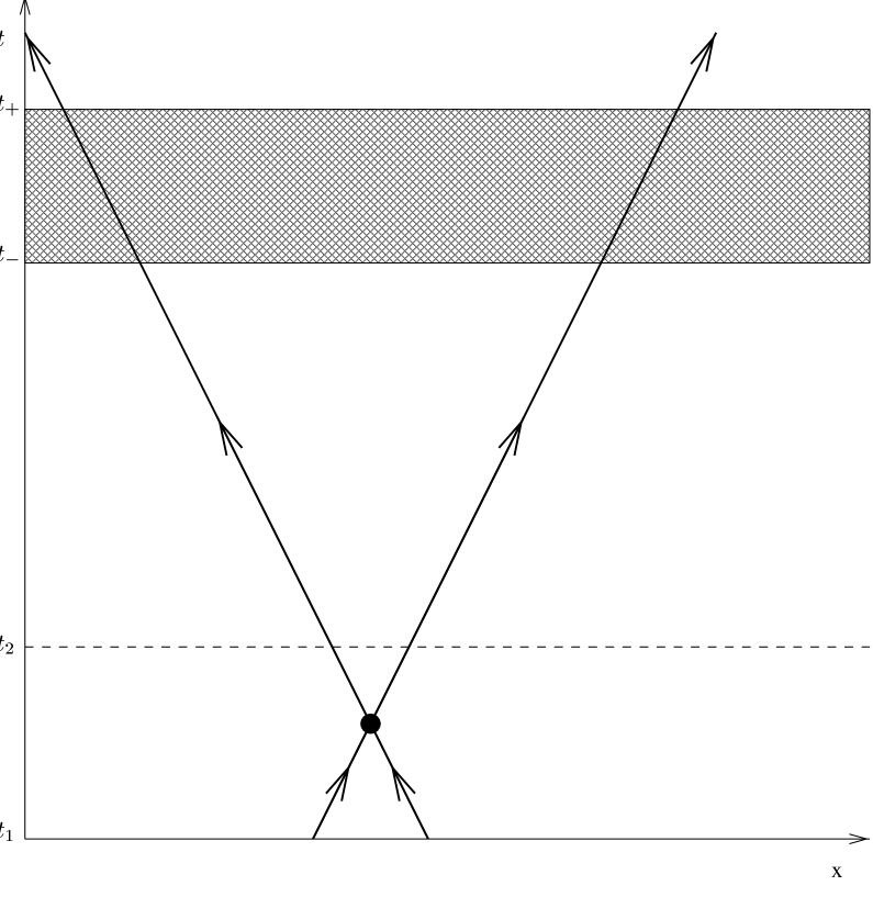
Figure 1: The scattering event and its background spacetime. The event takes place between $t_{1}$ and $t_{2}$, and the region of CTCs is between $t_{-}$ and $t_{+}$.

In generalized quantum mechanics it is not always possible to assign a probability to a given history. Two coarse-grained histories are said to decohere if the quantum interference between the two histories is zero. This quantum interference is measured by the decoherence functional, which is a complex functional of two coarse-grained histories. Probabilities can be defined for a given exhaustive coarse-graining only if every pair of histories in the coarse-graining decohere [2]. For this paper, we will assume that the weak coupling of “the experiment” to “the environment” will cause decoherence, and therefore all probabilities are well defined [10].

Since our probabilities are well defined, we may use generalized quantum mechanics to calculate the probability of a given coarse-grained history  [5]. We do so by stringing together a series of Heisenberg operators, as defined in (1), which act on our initial density matrix $\rho$. We simply insert the non-unitary operator, $X$, into the string according to when the region of CTCs occurs with respect to the various alternatives. Thus, the probability of an alternative $\alpha_{i}$ occurring when our initial density matrix is $\rho$ is given by

$$p(\alpha_{i})=\frac{Tr[XP_{\alpha_{i}}\rho P_{\alpha_{i}}X^{+}]}{Tr[X\rho X^{\dagger}]}\;,$$ (2)

where

$$X=U^{-1}(t_{+},t_{f})X_{s}U(t_{-},t_{1})$$

and $t_{f}$ is the final time, to the far future, where we trace over all final states. Equation (2) expresses the probability of a system beginning in a initial configuration represented by $\rho$, and at some point in the history, one or more variables which represent the system falling into a range corresponding to an alternative $\alpha_{i}$. The latter part is represented by the projection operator $P_{\alpha_{i}}$. The system then experiences non-unitary evolution due to the CTCs, and finally we sum over all possible final configurations.

The probability for a given history depends on the non-unitary evolution of the particles after the conclusion of the experiment. Thus, the theory is manifestly acausal. If there is no region of CTCs to the future of the experiment, the probability reduces to

$$p(\alpha_{i})=Tr[P_{\alpha_{i}}\rho P_{\alpha_{i}}]\;,$$ (3)

which is causal. We will now find the deviation in $p(\alpha_{i})$ if CTCs exist in the future of the experiment.

Since both $t_{1}$ and $t_{2}$ are before $t_{-}$, we can express $\rho$ and $P_{\alpha_{i}}$ in terms of quantum states at these times. For simplicity, we assume pure states:

$$\rho\!\!\! = \!\!\!|\phi\rangle\langle\phi|\;;$$ (4)

$$P_{\alpha_{i}}\!\!\! = \!\!\!|\psi_{i}\rangle\langle\psi_{i}|\;;$$

where $|\phi\rangle$,$|\psi_{i}\rangle$ are two-particle quantum states defined at $t_{1},t_{2}$ respectively. Substituting these into (2) we have

$$p(\psi_{i})=N\,Tr[X{|\psi_{i}\rangle}{\langle\psi_{i}|\phi\rangle}{\langle\phi|\psi_{i}\rangle}{\langle\psi_{i}|}X^{\dagger}]\;,$$ (5)

where

$$\frac{1}{N}=Tr[X|\phi\rangle\langle\phi|X^{\dagger}]\;.$$

We now explicitly write the probability in terms of single particle states.

$$|\psi_{i}\rangle\!\!\! = \!\!\!|\psi_{i1}\rangle\otimes|\psi_{i2}\rangle\;,$$ (6)

$$|\phi\rangle\!\!\! = \!\!\!|\phi_{1}\rangle\otimes|\phi_{2}\rangle\;.$$

We will assume that $X$ can be factored into two non-unitary operators $X_{1}$ and $X_{2}$, which evolve particles 1 and 2 respectively from $t_{-}$ to $t_{+}$:

$$X=X_{1}\otimes X_{2}\;.$$ (7)

This assumption is sensible as we expect the distance between particles after the scattering event to be large compared to the interaction range. Substituting (6) and (7) into (5), we have

$$P(\psi_{i})=N{|\langle\psi_{i}|\phi\rangle|}^{2}\langle\psi_{i1}|{X_{1}}^{\dagger}X_{1}|\psi_{i1}\rangle\langle\psi_{i2}|{X_{2}}^{\dagger}X_{2}|\psi_{i2}\rangle$$ (8)

Many authors [1, 3, 4] have shown that the operator which evolves a state from before a region of CTCs to after that region is non-unitary for interacting theories in perturbation theory. These authors showed that the non-unitary component of the evolution is due to particle interactions in the appropriate theory. When the evolution is expanded using perturbation theory, with a small parameter $\lambda$ associated with the interaction, the non-unitary component is of order $\lambda$ or higher. Thus, we write

$$X_{j}^{\dagger}X_{j}=1+\lambda\hat{\epsilon}_{j_{1}}+\lambda^{2}\hat{\epsilon}_{j_{2}}+...$$ (9)

where $j=(1,2)$. The $\epsilon_{j_{n}}$ are operators which express the non-unitary component of the evolution, and $\lambda$ is some small parameter. We will only examine the evolution to first order, so

$$X_{i}^{\dagger}X_{i}\approx 1+\lambda\hat{\epsilon}_{i_{1}}\equiv 1+\lambda\hat{\epsilon}_{i}\;,$$ (10)

To first order in $\lambda$,

$$P(\psi_{i})=N{|\langle\psi_{i}|\phi\rangle|}^{2}(1+\lambda\langle\psi_{i1}|{\epsilon}_{1}|\psi_{i1}\rangle)(1+\lambda\langle\psi_{i2}|{\epsilon}_{2}|\psi_{i2}\rangle)\;,$$ (11)

where

$$N^{-1}=(1+\lambda\langle\phi_{1}|{\epsilon}_{1}|\phi_{1}\rangle)(1+\lambda\langle\phi_{2}|{\epsilon}_{2}|\phi_{2}\rangle)\;.$$ (12)

Ignoring all terms of $o({\lambda}^{2})$ or higher, we get

$$P(\psi_{i})={|\langle\psi_{i}|\phi\rangle|}^{2}\left[\frac{1+\lambda(\langle\psi_{i1}|{\epsilon}_{1}|\psi_{i1}\rangle+\langle\psi_{i2}|{\epsilon}_{2}|\psi_{i2}\rangle)}{1+\lambda(\langle\phi_{1}|{\epsilon}_{1}|\phi_{1}\rangle+\langle\phi_{2}|{\epsilon}_{2}|\phi_{2}\rangle)}\right]\;.$$ (13)

We see that the standard transition amplitude is modified by a multiplicative factor. This factor depends on the non-unitary evolution that both the final and initial state experience as they pass between $t_{-}$ and $t_{+}$.

As noted before, if no CTCs exist in the experiment’s future, (13) reduces to

$$p(\psi_{i})={|\langle\psi_{i}|\phi\rangle|}^{2}\;.$$ (14)

This is the result predicted by standard quantum mechanics, which is causal.

3 The position dependence of $\langle\xi|\epsilon_{i}|\xi\rangle$

Equation (13) expresses the probability for a certain alternative to occur after a scattering event. Since this result depends on the non-unitary evolution that both the pre- and post-scattering states experience between $t_{-}$ and $t_{+}$ we must investigate this effect in detail in order to calculate the total cross section for a scattering experiment. The post-scattering trajectory of the particles, and their location at $t=t_{-}$ will depend on the scattering angle. Since the identified regions are spatially bounded, the non-unitary effect on a given particle may depend on the spatial distance between the particle and the identified region as the particle passes from $t=t_{-}$ to $t=t_{+}$. We let $|\xi\rangle$ represent a generic particle which, in our case, will be one of the particles from the scattering experiment. We will find the behavior of the non-unitary evolution which $|\xi\rangle$ experiences as a function of the particle’s distance from the center of the identified region.

There are many different spacetimes which contain CTCs. For our calculation we will use a 1+1 dimensional spacetime introduced by Politzer [1]. This spacetime is simple, yet has all the essential features of a spacetime with CTCs. We review the Politzer spacetime, which is shown in figure 2. The horizontal lines of length $L$, centered at $z=0$, at $t=t_{-}$ and $t=t_{+}$ are identified so that along them the region immediately before $t=t_{-}$ connects smoothly to that after $t=t_{+}$, while the region immediately before $t=t_{+}$ connects smoothly to that after $t=t_{-}$. We define $T\equiv t_{+}-t_{-}$, $Y\equiv(-\frac{L}{2},\frac{L}{2})$, and $R\equiv Y\otimes(t_{-},t_{+})$. We will refer to the identified regions as the time machine, and $R$ as the interior of the time machine. We will choose the spacetime to be non-relativistic, and flat everywhere, with the identification mentioned above. This spacetime contains a region of CTCs infinite in spatial extent, and bounded in time by $t=t_{-}$ and $t=t_{+}$.

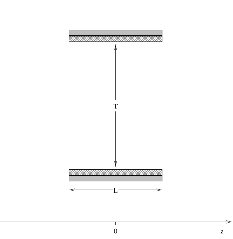
Figure 2: The Politzer time-machine spacetime in 1+1 dimensions. The two shadings represent the identification between the two horizontal lines at $t=t_{-}$ and $t=t_{+}$, so that $t<t_{-}$ connects smoothly with $t>t_{+}$ and $t<t_{+}$ connects smoothly with $t>t_{-}$.

Important notational convention: Throughout this section we will use the same position notation as Politzer [1]: $y$ variables refer to positions between $-{\frac{L}{2}}$ to $\frac{L}{2}$, while $x$ variables refer to positions outside that region and $z$ variables are unlimited.

After the scattering experiment the particles will evolve through time until $t=t_{-}$ at which point the particles will pass through the region of CTCs. In this region each particle may interact with a future version of itself or with a particle trapped inside the time machine. We expect that the inter-particle interaction will be short ranged such as a screened Coulomb force or a nuclear force. Thus we model the interaction with a contact potential $V(z,z^{\prime})=\lambda V_{0}\delta(z-z^{\prime})$. Although the scattering experiment itself will be considered in 3+1 dimensions in section 4, here we will look at the interaction which occurs as a single particle passes by the time machine in 1+1 dimensions for simplicity, and then generalize our result to 3+1 dimensions. This particle will be one of the pre- or post-scattering particles, which has evolved through time up to $t=t_{-}$. We will use bosons in non-relativistic quantum mechanics, with the standard, non-interacting, flat space propagator:

$$K_{f}(z_{2},t_{2};z_{1},t_{1})=\left\{\begin{array}[]{ll}{\left(\frac{m}{2\pi ih(t_{2}-t_{1})}\right)}^{\frac{1}{2}}\exp\left[\frac{im{(z_{2}-z_{1})}^{2}}{2\hbar(t_{2}-t_{1})}\right]&t_{2}>t_{1}\\ \delta(z_{2}-z_{1})&t_{2}=t_{1}\;.\\ 0&t_{2}<t_{1}\end{array}\right.$$ (15)

We will now find an expansion for $\langle\xi|{\epsilon}_{i}|\xi\rangle$, the non-unitary evolution $|\xi\rangle$ experiences through the region of CTCs, by using the Born approximation. We will expand the complete interaction diagrammatically and only look at terms which are first order in $\lambda$.

We define $K(z_{2},t_{2};z_{1},t_{1})$ as the amplitude for all paths which begin at $(z_{1},t_{1})$ and end at $(z_{2},t_{2})$. This includes all scatterings and all numbers of windings through the identified regions. Expanding $K$ order by order in $\lambda$, we get

$$K=K_{0}+\lambda K_{1}+{\lambda}^{2}K_{2}+...\;,$$ (16)

where $K_{i}$ is the piece of the amplitude which is ith order in the interaction.
Using our propagators we will now find an expression for $\langle x^{\prime}|\epsilon|x\rangle$, which will be used to find $\langle\xi|\epsilon|\xi\rangle$. Given our definition of $K$, we can expand $\langle x^{\prime}|X^{\dagger}X|x\rangle$ in terms of propagators:

$$\langle x^{\prime}|X^{\dagger}X|x\rangle = \int dx_{1}\,\langle x^{\prime}|X^{\dagger}|x_{1}\rangle\langle x_{1}|X|x\rangle\;,$$ (17)

$$= \int dx_{1}\,K^{\ast}(x_{1},t_{+};x^{\prime},t_{-})K(x_{1},t_{+};x,t_{-})\;.$$

Arranging the terms order by order in $\lambda$,

$$\langle x^{\prime}|X^{\dagger}X|x\rangle = \int dx_{1}\left[K_{0}^{\ast}(x_{1},t_{+};x^{\prime},t_{-})K_{0}(x_{1},t_{+};x,t_{-})\right.$$ (18)

$$+\;\lambda\left(K_{0}^{\ast}(x_{1},t_{+};x^{\prime},t_{-})K_{1}(x_{1},t_{-};x,t_{-})\right.$$

$$+\left.\left.K_{1}^{\ast}(x_{1},t_{+};x^{\prime},t_{-})K_{0}(x_{1},t_{+};x,t_{-})\right)+o(\lambda^{2})\right]\;.$$

$K_{0}$ is a free propagator, therefore

$$\int dx_{1}\,K_{0}^{\ast}(x_{1},t_{+};x^{\prime},t_{-})K_{0}(x_{1},t_{+};x,t_{-})=\delta(x^{\prime},x)\;.$$ (19)

If we define

$$A(x,x^{\prime})\equiv\int dx_{1}\,K_{0}^{\ast}(x_{1},t_{+};x^{\prime},t_{-})K_{1}(x_{1},t_{+};x,t_{-})\;,$$ (20)

and throw away terms $o(\lambda^{2})$ and higher, then (18) becomes

$$\langle x^{\prime}|X^{\dagger}X|x\rangle\approx\delta(x^{\prime},x)+\lambda[A(x,x^{\prime})+A^{\ast}(x^{\prime},x)]\;.$$ (21)

Comparing (21) to (10), we find

$$\langle x^{\prime}|\epsilon|x\rangle=A(x,x^{\prime})+A^{\ast}(x^{\prime},x)\;.$$ (22)

We ignore terms $o(\lambda^{2})$ and higher, since we are using the Born approximation. We wish to investigate the non-unitary evolution in equation (13), which is expressed by terms of the form $\langle\xi|\epsilon|\xi\rangle$, where $|\xi\rangle$ is a single-particle state.

$$\langle\xi|\epsilon|\xi\rangle = \int\!\!\int dx\,dx^{\prime}\,\xi(x,t_{-})[A(x,x^{\prime})+A^{\ast}(x^{\prime},x)]\xi^{\ast}(x^{\prime},t_{-})$$ (23)

$$= 2\,{\rm Re}\left[\langle\xi|A|\xi\rangle\right]$$

$K_{i}$ includes every number of windings through the identified regions. Each $K_{i}$ can be expanded as a series, where each subsequent term represents another winding through the time machine. For example, the expansion for $K_{0}$, illustrated in figure 3, is

$$K_{0}(x^{\prime},t_{+};x,t_{-})=K_{f}(x^{\prime},t_{+};x,t_{-})+\int_{-\frac{L}{2}}^{\frac{L}{2}}dyK_{f}(x^{\prime},t_{+};y,t_{-})K_{f}(y,t_{+};x,t_{-})$$

$$+\int_{-\frac{L}{2}}^{\frac{L}{2}}\int_{-\frac{L}{2}}^{\frac{L}{2}}dy\,dy^{\prime}K_{f}(x^{\prime},t_{+};y,t_{-})K_{f}(y,t_{+};y^{\prime},t_{-})K_{f}(y^{\prime},t_{+};x,t_{-})+...$$ (24)

Figure 3: The first three diagrams in the expansion of $K_{0}(x^{\prime},t_{+};x,t_{-})$ in terms of number of windings through the time machine. The figure includes diagrams with winding number 0, 1, and 2.

As we see in (20), $A(x,x^{\prime})$ can be expressed in terms of the $K_{i}$’s. Therefore, $A(x,x^{\prime})$ is also the sum of an infinite number of terms. We will initially simplify the calculation as Politzer does [1] by assuming $\hbar T>>mL^{2}$. For a given $K_{i}$, each subsequent term has another winding through the time machine and therefore another integral over $y$. The assumption $\hbar T>>mL^{2}$ can be interpreted as choosing $T$ and $L$ such that the wave packet spreads significantly compared to $L$ during the time $T$. For each additional winding through the identified regions, more of the wave packet will spread outside $Y$ and not return to $t_{-}$ to wind through again. Thus, for each subsequent winding, less and less of the wave packet will remain to contribute to the non-unitary evolution of the next winding. Thus any given term in the expansion is smaller than the previous term by a factor of the small parameter $\frac{mL^{2}}{\hbar T}$. We can therefore approximate each $K_{i}$ by the first term in its expansion, i.e., the term with the lowest number of windings. With this assumption, the diagrammatic representation for $A(x,x^{\prime})$ is shown below in figure 4.

Figure 4: The diagrammatic representation of $A(x,x^{\prime})$: the $o(\lambda)$ term in the expansion of $\langle x^{\prime}|X^{\dagger}X|x\rangle$. Lines with forward (backward) pointing arrows denote factors of $K_{f}$ ($K_{f}^{\ast}$), the heavy horizontal lines denote the identified surfaces, and the dot denotes a factor of $\lambda V_{0}$.

Since we are interested in estimating the dependence of $\langle\xi|A|\xi\rangle$ on the particle’s spatial distance from the center of $Y$, we will take $|\xi\rangle$ to be a stationary Gaussian wave packet centered at $x=x_{c}$ with width $d$:

$$\xi(x,t_{-})=\pi^{-\frac{1}{4}}d^{-\frac{1}{2}}\exp\left[\frac{-(x-x_{c})^{2}}{2d^{2}}\right]\;.$$ (25)

We are looking for the dependence of $\langle\xi|A|\xi\rangle$ on $x_{c}$ for large $x_{c}$. Thus we assume

$$x_{c} >> L\;,$$

$$x_{c} >> d\;,$$ (26)

$$x_{c} >> \frac{\hbar T}{m}\;.$$

An expression for $\langle\xi|A|\xi\rangle$ is found from its diagrammatic representation. The full calculation is completed in the appendix, and the dependence on $x_{c}$ extracted. In essence, the integral is an overlap between $|\xi\rangle$ and a particle caught in $R$. Since we are using a contact potential, the overlap integral will fall off exponentially as the Gaussian wave packet is moved farther from the time machine. Thus, the dominant $x_{c}$ behavior is found to be

$$\langle\xi|\epsilon|\xi\rangle=2\,{\rm Re}\left[\langle\xi|A|\xi\rangle\right]\propto\exp\left[\frac{-x_{c}^{2}}{d^{2}}\left(\frac{2R^{2}+1}{2(R^{2}+1)}\right)\right]\;,$$ (27)

where

$$R=\frac{md^{2}}{\hbar T}\;.$$

Due to the contact potential, the non-unitary evolution of $|\xi\rangle$ is proportional to the overlap between the wave packet and the region $Y$. We interpret the result above to mean that the effect falls off exponentially with the spatial distance between the center of the wave packet and the center of $Y$. Therefore, we expect $\langle\xi|\epsilon|\xi\rangle\approx 0$ unless there is a significant overlap between the wave packet and the region $Y$. If $d<L$, the width of the wave packet is smaller than that of $Y$, and we expect a significant overlap only when the center of the wave packet is inside $R$, i.e. $\langle\xi|\epsilon|\xi\rangle\approx 0$ unless $|x_{c}|<\frac{L}{2}$ for some time between $t=t_{-}$ and $t=t_{+}$. If $L<d$, the width of the particle is larger than that of the time machine, and we expect that $\langle\xi|\epsilon|\xi\rangle$ may be significant even if $|x_{c}|>\frac{L}{2}$. In this case, we expect the overlap between the wave packet and the region $(-\frac{L}{2},\frac{L}{2})$ to be non-negligible as long as the wave packet is positioned such that the center of $Y$ lies a distance less than $d$ from the center of the wave packet.

Now we generalize our result to include the case when the minimal winding approximation ($\hbar T>>mL^{2}$) does not hold. In this case, there are an infinite number of $o(\lambda)$ terms in our expansion for $\langle\xi|\epsilon|\xi\rangle$. These terms represent all possible numbers of windings through the identification, and each term can be represented by a diagram. The summation of these terms is non-trivial. However, we are only interested in the dependence of $\langle\xi|\epsilon|\xi\rangle$ on $x_{c}$ for large $x_{c}$. In each term of the expansion $x_{c}$ will appear only in $\xi(x)$ and $\xi^{\ast}(x)$. Thus, the dependence of each term on $x_{c}$ will only come from $\xi(x)$, $\xi^{\ast}(x)$, and the propagators which connect the external wave packets to the time machine. The propagators which connect one identified region to the other, or one of the identified regions to the interaction point will not contribute the to the $x_{c}$ dependence of the term. We will therefore organize the infinite set of diagrams into 3 distinct classes. Each diagram has two external propagators which connect $\xi(x)$ and $\xi^{\ast}(x)$ to the identified regions. Since we are limiting our expansion to $o(\lambda)$ each term will be represented by a diagram with only one interaction point. The three classes will be the sets of diagrams where both, one, or neither of the external propagators connect to the interaction point. We will call these classes A,B, and C respectively. The lowest winding diagrams are shown below in figure 5, grouped by class.

Figure 5: The diagrams of $o(\lambda)$ with the lowest numbers of windings through the identification in the expansion of $\langle\xi|\epsilon|\xi\rangle$. These diagrams are split into three classes: A, B, and C, which include diagrams with two, one, or zero external propagators connected to the interaction point respectively. The interaction point in each diagram is denoted by a black dot. The intersection of two propagator lines without a dot does not represent an interaction. The ${K_{f}}^{\ast}$ term is suppressed in each diagram.

As discussed above, all diagrams in a given class will have the same dependence on $x_{c}$. The $x_{c}$ dependence of diagram (A.i) was calculated in the appendix, and is shown in (27). Therefore, all diagrams in class A behave like $\exp\left(-\frac{x_{c}^{2}}{d^{2}}\right)$ for large $x_{c}$. Similar calculations were done for diagrams (B.i) and (C.i). Both were found to behave like $\exp\left(-\frac{x_{c}^{2}}{d^{2}}\right)$ for large $x_{c}$, and so all $o(\lambda)$ diagrams are dominated by a factor of $\exp\left(-\frac{x_{c}^{2}}{d^{2}}\right)$ for large $x_{c}$. Therefore, all conclusions made about the non-unitary evolution for the minimal winding case ($\hbar T>>mL^{2}$) also hold when all windings are included. Since the non-unitary component of the evolution drops off exponentially with the spatial distance between the wave packet and $Y$, the non-unitary component of the evolution will be non-negligible only if the particle passes through $R$, the region of spacetime between the identified surfaces.

4 The cross-section of a scattering experiment with a region of CTCs in the experiment’s future

In section 2 we found that a region of CTCs could alter the probability assigned to a given history, even if the region of CTCs was in the future of the last alternative in the history. Equation (13) expresses how the CTCs alter the probability of any transition occurring before them. In section 3 we found that for histories which involve wave packets $\langle\xi|\epsilon|\xi\rangle\approx 0$, unless there is significant overlap between the wave packet and the region $R$. For particles smaller than the identified spatial region, this means that the particle must pass through $R$: the region of spacetime between the two identified regions. We will now examine a scattering experiment, which provides us with states with well known trajectories. By examining which pre- and post-scattering states pass through $R$, we will calculate the effect which the CTCs have on the total cross-section.

The spacetime chosen here will be the same as that of section 3 except that we will be working in 3+1 dimensions. We choose a ball of diameter $L$, centered at a point $p$, and label this region $Y^{3}$. An identification is made between $Y^{3}$ at $t=t_{-}$ and $Y^{3}$ at $t=t_{+}$. We define $R^{3}\equiv Y^{3}\otimes(t_{-},t_{+})$. We assume our initial density matrix $\rho$ has been prepared at $t=0$, and that it describes a system of two particles, each with mass $m$. The particles are aimed at each other, each with speed $v$ as measured from the lab frame. Therefore, $\vec{P}_{tot}=0$, and the scattering will be spherically symmetric. As we are only interested in estimating this effect, we will assume a semi-classical picture for the particles: the position and momentum of each particle are reasonably well known. At time $t_{2}$, after the scattering, the system is in the state $|\psi_{i}\rangle$. Examination of the initial and final states allows us to deduce the location of the scattering center: $(x_{s},t_{s})$. The spatial distance between the scattering center and point $p$ is $D$, while the time difference between the scattering event and the first identified region, $t_{-}-t_{s}$, we will call $\cal{T}$. This setup is shown below in figure 6.

Figure 6: The scattering event and its location with respect to the Politzer identification. The event takes place in 3+1 dimensions, so two spatial dimensions are suppressed.

Equation (13) shows that the transitional probability $p(\psi_{i})$ is equal to the product of ${\left|\langle\psi_{i}|\phi\rangle\right|}^{2}$, the transitional probability if no CTCs exist, and some factor which represents the non-unitary evolution of both the pre- and post-scattering states:

$$p(\psi_{i})=g(\psi_{i},\phi){\left|\langle\psi_{i}|\phi\rangle\right|}^{2}\;,$$ (28)

where

$$g(\psi_{i},\phi)\equiv\frac{1+\lambda(\langle\psi_{i1}|{\epsilon}_{1}|\psi_{i1}\rangle+\langle\psi_{i2}|{\epsilon}_{2}|\psi_{i2}\rangle)}{1+\lambda(\langle\phi_{1}|{\epsilon}_{1}|\phi_{1}\rangle+\langle\phi_{2}|{\epsilon}_{2}|\phi_{2}\rangle)}\;.$$

From scattering theory we know that the differential cross-section,$\left(\frac{d\sigma}{d\Omega}\right)$, is directly proportional to the transitional probability:

$$\left(\frac{d\sigma}{d\Omega}\right)=Kp(\psi_{i})\;.$$ (29)

The same relationship holds true if the CTCs do not exist. Let $\left(\frac{d\sigma}{d\Omega}\right)_{0}$ be the differential cross-section if CTCs do not exist,

$$\left(\frac{d\sigma}{d\Omega}\right)_{0}=K{\left|\langle\psi|\phi\rangle\right|}^{2}\;.$$ (30)

Where we will suppress the index $i$ from now on. Combining (28) and (29) we see that our differential-cross section is related to the standard (no CTC) differential cross-section by the same factor $g(\psi,\phi)$ which relates $p(\psi)$ and ${\left|\langle\psi|\phi\rangle\right|}^{2}$.

We integrate over $d\Omega$ to get the total cross-section.

$$\sigma = \int_{4\pi}\left(\frac{d\sigma}{d\Omega}\right)d\Omega\;,$$ (31)

$$= \int_{4\pi}\left(\frac{d\sigma}{d\Omega}\right)_{0}g(\psi,\phi)\,d\Omega\;,$$

$$= \int_{4\pi}\left(\frac{d\sigma}{d\Omega}\right)_{0}\left[\frac{1+\lambda(\langle\psi_{1}|{\epsilon}_{1}|\psi_{1}\rangle+\langle\psi_{2}|{\epsilon}_{2}|\psi_{2}\rangle)}{1+\lambda(\langle\phi_{1}|{\epsilon}_{1}|\phi_{1}\rangle+\langle\phi_{2}|{\epsilon}_{2}|\phi_{2}\rangle)}\right]d\Omega\;.$$

The initial states, $|\phi_{1}\rangle$ and $|\phi_{2}\rangle$, are independent of the scattering angle, while the post-scattering states $|{\psi}_{1}\rangle$ and $|{\psi}_{2}\rangle$, depend on the scattering angle. Thus, only the post-scattering states will vary as we integrate over $d\Omega$.

$$\sigma = \frac{1}{1+\lambda(\langle\phi_{1}|{\epsilon}_{1}|\phi_{1}\rangle+\langle\phi_{2}|{\epsilon}_{2}|\phi_{2}\rangle)}\int_{4\pi}\left(\frac{d\sigma}{d\Omega}\right)_{0}\left[1+\lambda(\langle\psi_{1}|{\epsilon}_{1}|\psi_{1}\rangle+\langle\psi_{2}|{\epsilon}_{2}|\psi_{2}\rangle)\right]\,d\Omega,$$ (32)

$$= \frac{1}{1+\lambda(\langle\phi_{1}|{\epsilon}_{1}|\phi_{1}\rangle+\langle\phi_{2}|{\epsilon}_{2}|\phi_{2}\rangle)}\left[\sigma_{0}+\lambda\int_{4\pi}\left(\frac{d\sigma}{d\Omega}\right)_{0}\langle\psi_{1}|{\epsilon}_{1}|\psi_{1}\rangle\,d\Omega\right.$$

$$\qquad\qquad\qquad\qquad\qquad\qquad\qquad\;\;\;+\left.\lambda\int_{4\pi}\left(\frac{d\sigma}{d\Omega}\right)_{0}\langle\psi_{2}|{\epsilon}_{2}|\psi_{2}\rangle\,d\Omega\right]\;.$$

Where $\sigma_{0}$ is the total cross-section if CTCs do not exist.

As discussed in section 3, for a given wave packet $|\xi\rangle$, $\langle\xi|\epsilon|\xi\rangle\approx 0$ unless a significant portion of the wave packet passes through $R^{3}$. This will only occur for certain values of the particle’s momentum. First, only a limited range of particle speeds will enable the particle to reach $Y^{3}$ between $t=t_{-}$ and $t=t_{+}$. The trajectory of the particle represented by $|\xi\rangle$ must lie inside the shaded region shown in figure 7, in order for $\langle\xi|\epsilon_{j}|\xi\rangle$ to be non-negligible.

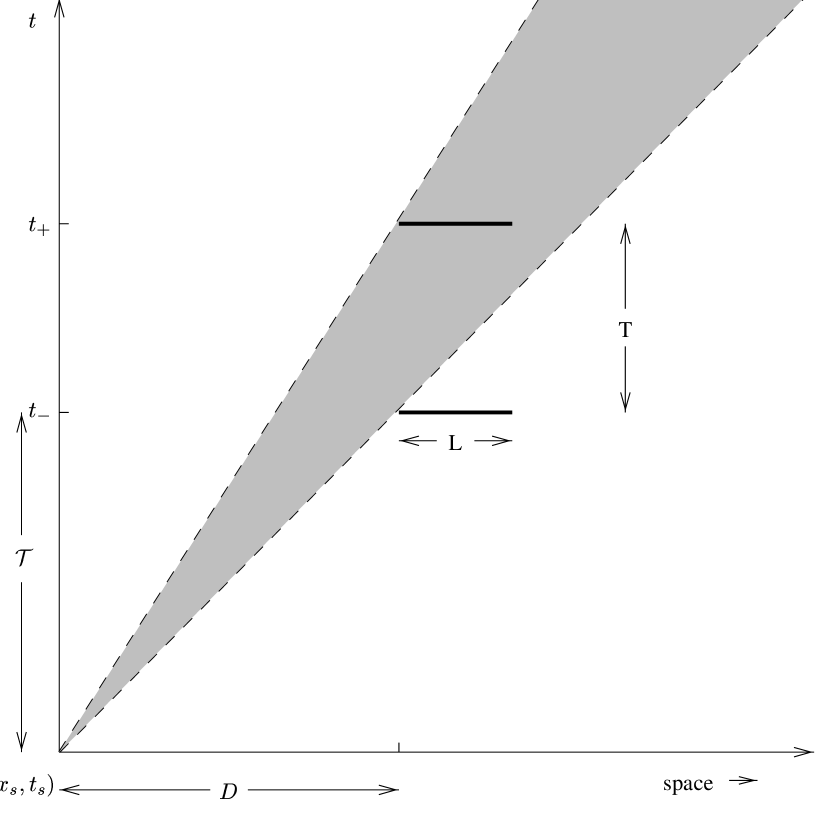
Figure 7: An illustration of the range of speeds for a post-scattering particle which lead to a possible non-unitary effect. The particle’s trajectory must pass through the shaded area in order for the particle to have any chance of passing inside the time machine.

This leads to the following range for $v_{i}$, the speed of the particle in question:

$$\frac{D}{\cal{T}}<v_{i}<\frac{D}{{\cal{T}}+T}\;.$$ (33)

Due to our chosen initial condition $v_{10}=v_{20}=v_{1f}=v_{2f}=v$. For now, we assume that $v$ falls within this range. Even if this condition is met, the particle must be traveling towards $Y^{3}$ in order to pass inside it. This will have different consequences for the pre- and post-scattering particles, since we will integrate over all final angles that the the post-scattering particles scatter into. The trajectories of the initial particles are fixed once the initial state is chosen. Therefore, if neither of the initial particles is aimed at $Y^{3}$ then $\langle\phi_{j}|\epsilon|\phi_{j}\rangle\approx 0\,,\;(j=1,2)$. For now, we will assume this to be the case and examine the effect on the total cross-section due to the post-scattering particles only. With this assumption equation (32) becomes

$$\sigma=\sigma_{0}+\lambda\int_{4\pi}\left(\frac{d\sigma}{d\Omega}\right)_{0}\langle\psi_{1}|{\epsilon}_{1}|\psi_{1}\rangle\,d\Omega+\lambda\int_{4\pi}\left(\frac{d\sigma}{d\Omega}\right)_{0}\langle\psi_{2}|{\epsilon}_{2}|\psi_{2}\rangle\,d\Omega\;.$$ (34)

We define

$$(\Delta\sigma)_{j}\equiv\lambda\int_{4\pi}\left(\frac{d\sigma}{d\Omega}\right)_{0}\langle\psi_{j}|{\epsilon}_{j}|\psi_{j}\rangle\,d\Omega\;,$$ (35)

where $j=(1,2)$, as the the change in the total cross-section due to particle $j$. The post-scattering particles must also be aimed at the time machine in order for $\langle\psi_{ij}|\epsilon_{j}|\psi_{ij}\rangle$ to be significant. To find the total cross-section, we will integrate over $d\theta\,d\phi$, which represents all angles which one of the particles could scatter into. The other particle will, in this case, simply scatter off the scattering center with an angle $\pi$ relative to the first particle. For a given particle, only a fraction of post-scattering angles will direct the particle towards $Y^{3}$. This fraction, $F$, is the fraction of the sphere subtended by the time machine as viewed from the scattering center. $F$ is related to $\Omega_{tm}$, the solid angle subtended by $Y^{3}$ as viewed from the scattering center. $\Omega_{tm}$ is illustrated in figure 8. $F$ is given in terms of $\Omega_{tm}$ by

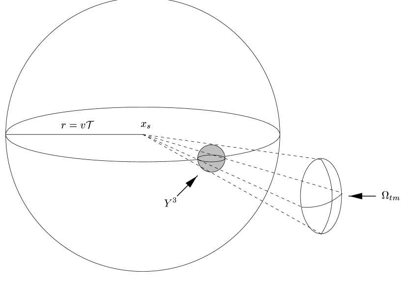
Figure 8: The solid angle subtended by $Y^{3}$ as viewed from the scattering center is $\Omega_{tm}$. Only post-scattering states aimed towards $Y^{3}$ will experience any non-unitary evolution.

$$F=\frac{\Omega_{tm}}{\Omega_{tot}}=\frac{\pi{\left(\frac{L}{2}\right)}^{2}}{4\pi D^{2}}=\frac{L^{2}}{16D^{2}}\;.$$ (36)

When we integrate equation (35) over $d\theta\,d\phi$, $\langle\psi_{j}|{\epsilon}_{j}|\psi_{j}\rangle\approx 0$ unless the element of the sphere which we are integrating over is contained in the fraction of the sphere subtended by $Y^{3}$.

$$(\Delta\sigma)_{j}=\lambda\int_{\Omega_{tm}}\left(\frac{d\sigma}{d\Omega}\right)_{0}\langle\psi_{j}|{\epsilon}_{j}|\psi_{j}\rangle\,d\theta\,d\phi\;,\;j=(1,2)\;.$$ (37)

However, $\langle\psi_{j}|{\epsilon}_{j}|\psi_{j}\rangle$ is not constant over the fraction of the sphere subtended by $Y^{3}\,$. As shown in the appendix,

$$\langle\psi_{j}|{\epsilon}_{j}|\psi_{j}\rangle\approx\frac{-2V_{0}}{\pi}{\left(\frac{m^{3}}{\hbar^{5}T^{3}}\right)}^{\frac{1}{2}}h(d,L)\,{T^{\prime}}^{3}\;,\;h(d,L)=\left\{\begin{array}[]{ll}1&d<<L\\ \frac{L}{ed}&L>>d\end{array}\right.\,.$$ (38)

Here $T^{\prime}$ is the time spent by the particle in $Y^{3}$. Let us define $S$ to be the length of the particle’s path inside $Y^{3}$, which $T^{\prime}$ is clearly dependent on. Assuming the particle does not wind through the identification , $S$ will vary with the $\theta$ and $\phi$ which the particle is scattered into. If we align our $\theta=0$ axis along the line connecting the scattering center and point $p$, we have azimuthal symmetry, and find

$$S=\left(L^{2}-4D^{2}{\sin^{2}\theta}\right)^{\frac{1}{2}}$$

and

$$T^{\prime}=\frac{\left(L^{2}-4D^{2}\sin^{2}\theta\right)^{\frac{1}{2}}}{v}\;.$$ (39)

Substituting (39) and (38) into (37) we find

$$(\Delta\sigma)_{j}=\frac{-2\lambda V_{0}h(d,l)}{\pi v^{3}}{\left(\frac{m^{3}}{\hbar^{5}T^{3}}\right)}^{\frac{1}{2}}\int_{\Omega_{tm}}\left(\frac{d\sigma}{d\Omega}\right)_{0}\left(L^{2}-4D^{2}{\sin^{2}\theta}\right)^{\frac{3}{2}}\sin\theta\,d\theta\,d\phi\;.$$ (40)

Due to our choice of spherically symmetric scattering event, we know

$$\left(\frac{d\sigma}{d\Omega}\right)_{0}=\frac{\sigma_{0}}{4\pi}\;.$$ (41)

However, if the scattering is not spherically symmetric, then we simply substitute the correct expression in for $\left(\frac{d\sigma}{d\Omega}\right)_{0}$.

Combining equations (37), (38), (39), (36), and (41) we find

$$(\Delta\sigma)_{j}=\sigma_{0}\left\{\frac{-2\lambda V_{0}h(d,L)}{\pi v^{3}}{\left(\frac{m^{3}}{\hbar^{5}T^{3}}\right)}^{\frac{1}{2}}\frac{L^{5}}{40D^{2}}\left[1-\left(\frac{L^{2}}{L^{2}+4D^{2}}\right)^{\frac{5}{2}}\right]\right\}\;.$$ (42)

The effect will be the same for each of the two particles, so $(\Delta\sigma)_{1}=(\Delta\sigma)_{2}$. Therefore

$$\sigma=\sigma_{0}\left\{1-\frac{\lambda L^{5}V_{0}}{10\pi D^{2}v^{3}}{\left(\frac{m^{3}}{\hbar^{5}T^{3}}\right)}^{\frac{1}{2}}h(d,L)\left[1-\left(\frac{L^{2}}{L^{2}+4D^{2}}\right)^{\frac{5}{2}}\right]\right\}\;.$$ (43)

We have arrived at an expression for the deviation in the total cross- section of a scattering experiment with a region of CTCs in its future. This expression assumes that neither pre-scattering particle is aimed towards $Y^{3}$ and that the velocity of the particles is within the range specified in (33).

We have shown that with Hartle’s prescription for calculating probabilities in spacetimes with CTCs the total cross-section of a scattering experiment before the region of CTCs will deviate from the standard (no CTCs) value as shown in (43). The question now arises: will this effect be large enough to be measured in a typical scattering experiment? We will now give an estimate of the size of this effect for a few cases. If topological or geometric defects which cause CTCs are allowed by the laws of physics we expect that the scale for naturally occurring defects will be the Planck scale, for both time and space [11, 12]. We will model a defect of this kind using a Planck-scale Politzer time machine. We plug in reasonable values for electron-electron scattering into (43) and take a Planck-scale time machine a Planck length away from the scattering center. If we assume that the condition on the velocity of the electrons given in (33) is met, then the deviation in the total cross-section is approximately $1$ part in $10^{80}$. If the Planck-scale time machine is $1$ meter from the scattering center, the deviation drops to $1$ part in $10^{150}$. If we include the possibility of man-made time machines, which could be of a size traversable by humans [13, 14], then the deviation becomes larger. For a identified region 1 meter from the scattering center with $L=1\,$m and $T=1\,$s, the deviation is $1$ part in $10^{15}$. For the purpose of comparison to typical experimental error of total cross-sections we will use the measurement of the anomalous magnetic moment of the electron, which has an accuracy of $1$ part in $10^{11}$ [15]. We will use this result as a upper bound on the sensitivity of total cross-section measurements. Therefore, the deviation we have calculated in the total-cross section due to a Politzer time machine in our future is negligible compared to the experimental error associated with the measurement. Therefore, even if the time machine is located such that (33) is satisfied it would be impossible to detect a single Planck-scale or human-scale time machine in our future from its effect on the total cross-section of a scattering event.

If multiple time machines exist, then for a given scattering event the only ones which will contribute to a deviation in the total cross-section will be those located such that the velocity of the particles satisfies (33). We have found that the effect is additive for multiple time machines which satisfy this condition. Again, we assume that neither of the pre-scattering particles are aimed at any of the time machines which contribute to the deviation. The total cross section for a specific scattering event can be computed by selecting only the time machines for which the velocity satisfies (33), calculating the deviation in the total cross-section for each time machine using (43) and adding the deviations for all the time machines selected. Therefore, the more time machines we have in our future, the greater the chance of observing a deviation in the total cross-section of a scattering event in our present, as long as neither pre-scattering particle is aimed at a time machine. For a given event, if there are more time machines then there is a greater chance that enough time machines will be at correct locations in spacetime to satisfy (33) and cause a measurable deviation.

Because of the additive effect it is possible for a distribution of time machines throughout spacetime to cause a deviation in the total cross-section of a scattering event which would be measurable. In general, we cannot place limits on size, number or proximity of time machines, because for any given values for these quantities, it would be possible to design a configuration of time machines such that (33) was not satisfied for a given set of scattering events. In other words, the time machines could be distributed such that the particles involved in the scattering events would never pass inside any of the time machines, and therefore no deviation in the total cross-section would occur. Also, these results are only valid if neither pre-scattering particle is aimed at any of the contributing time machines . What is possible, however, is to rule out specific spacetime distributions of time machines in light of specific scattering experiments. For example, if we take an electron-electron scattering experiment for which the measured total cross-section agrees with the standard predicted result (no CTCs) within the experimental error, then we can rule out a spacetime which has either Planck-scale or human-scale time machines everywhere in spacetime except for the region of spacetime which surrounds the trajectory of the pre-scattering particles. When we calculate the deviation in the total cross-section due this distribution using (32), we find that the term in the numerator, which comes from integrating the non-unitary effect over all the post-scattering states is infinite. Due to lack of time machines in the path of the initial particle, the term in the denominator, which represents the non-unitary effect of the pre-scattering particles, is simply $1$. Therefore, Hartle’s prescription predicts an infinite deviation in the total cross section in this case, which is clearly absurd, so such spacetimes are ruled out.

The same result ensues if instead of the spacetime discussed above we have an expanding shell of time machines: at any given moment in time there is a spherical distribution of time machines around the scattering center at the same radius as the post-scattering particles. Again, the region surrounding the trajectory of the pre-scattering particles is empty. This distribution of time machines has an identical effect as the previous distribution, since this distribution is simply the subset of time machines in the previous example for which the particles’ velocity satisfies (33). It is also possible to imagine finite versions of these examples which would cause measurable deviations in the total cross-section. For either of the examples above, a finite distribution of time machines would lead to a measurable deviation in the total cross-section section of a given experiment if the radius of the distribution is large enough. For Planck-sized time machines, the radius of the distribution must be approximately $10^{16}$ light years which is extremely large. However, a distribution of human-scale time machines (with the dimensions discussed above) centered on the the scattering event need only have a radius of 10 km in order to cause a measurable deviation in the total cross section. If the distribution is not centered on the event, or is at a distance from the scattering event, the effect is diminished, and therefore we need a larger distribution in order for the deviation to be measurable. If Hartle’s prescription for applying generalized quantum mechanics to spacetimes with CTCs is correct, then spacetimes with any of these distributions of CTCs must be disallowed. For reasonably sized time machines, one needs a large number of time machines in close proximity to the scattering center in order for a measurable deviation in the total cross-section to occur. Clearly, there are a number of realistic distributions of Politzer time machines which would lead to deviations in the total cross section which are minute compared to the experimental error of any given scattering experiment. If the time machines are small, far away, or sparsely distributed, then it is very possible that a region of CTC’s could go completely unnoticed.

Some authors [11, 12] have asserted that quantum gravity predicts that at the Planck scale, spacetime is filled with CTCs. One possibility is that spacetime can be viewed as a quantum foam, with Planck-scale CTCs throughout spacetime. Another hypothesis is that CTCs will become prevalent during the big bang and the big crunch, due to quantum gravitational effects which are large at these times. We can model these possibilities simply with Planck-scale Politzer time machines which pervade spacetime. In any of these cases one might expect a significant deviation in the total cross-section of a scattering experiment due to the dense distribution of time machines. However, as we will show, this is not the case. Each of these cases involves an isotropic distribution of time machines: all pre- and post-scattering particles will pass through the same distribution of time machine. We will now use (32) to examine the total cross section of a scattering event. We will assume that $\langle\xi_{i}|\epsilon_{i}|\xi_{i}\rangle$ is the total non-unitary effect of all time machines which affected the particle $|\xi_{i}\rangle$. ($|\xi_{i}\rangle$ is generic and could be any of the pre- or post-scattering particles.) $\langle\xi_{i}|\epsilon_{i}|\xi_{i}\rangle$ will be identical for all states, including all pre-scattering states, and all possible post-scattering states, since the distribution of time machines is isotropic. When we calculate the total cross-section using (32), the integrals over $d\theta\,d\phi$ give factors of $4\pi$, which leads to the result:

$$\sigma^{\prime}=\sigma$$ (44)

Thus, when the distribution of time machines is isotropic, there is a cancellation effect, and the predicted total cross-section agrees with result expected if no CTCs existed. We see that this is a limiting case as $\Omega_{ctc}$ approaches $4\pi$. Therefore, we also expect the effect to be small if the distribution is nearly isotropic, or if only a small fraction of the solid angle has a different distribution of CTCs. In this case we would expect the effect caused by the initial and final particles to be nearly identical as long as the initial particles are not aimed at the small fraction of solid angle with a different distribution of time machines from the rest.

5 Acknowledgements

The author would like to thank A. Anderson, D. Craig, D. Deutch, C. Fewster, J. Friedman, S. Hawking, S. Kolitch, D. Politzer, and J. Simon for their helpful comments and conversations. Special thanks are given to H. A. C. Chamblin, S. Ross, and J. S. Whelan for their time and support. Finally, the author would like to thank his advisor, J. B. Hartle, for without his help and patience this paper would never have been finished.

Appendix A Appendix

We will be using the same notation for position coordinates $x,y,$ and $z$ as in section 3. Combining (20) and (23) we have

$$\langle\xi|A|\xi\rangle=\int\!\!\int dx\,dx^{\prime}\xi(x,t_{-})\left[\int dx_{1}K_{0}^{\ast}(x_{1},t_{+};x^{\prime},t_{-})K_{1}(x_{1},t_{+};x,t_{-})\right]\xi^{\ast}(x^{\prime},t_{-})\;.$$ (45)

where $K_{0}$ and $K_{1}$ are the amplitudes which are 0th and 1st order in the interaction respectively. As discussed previously, if we take the minimal winding approximation ($mL^{2}<<\hbar T$), $\langle\xi|A|\xi\rangle$ can be represented by the diagram shown in figure 4. This leads to the following expression for $\langle\xi|A|\xi\rangle$:

$$\langle\xi|A|\xi\rangle = -\frac{i}{\hbar}\int\!\!\int dx\,dx^{\prime}\int_{t_{-}}^{t_{+}}dt\int\!\!\int dz\,dx_{1}\int_{-\frac{L}{2}}^{\frac{L}{2}}dy\,K_{f}(z,t;x,t_{-})K_{f}(z,t;y,t_{-})$$ (46)

$$\times V_{0}K_{f}(y,t_{+};z,t)K_{f}(x_{1},t_{+};z,t)K_{f}^{\ast}(x_{1},t_{+};x^{\prime},t_{-})\xi(x,t_{-})\xi^{\ast}(x^{\prime},t_{-})\;.$$

Now,

$$\int dxK_{f}(z,t;x,t_{-})\xi(x,t_{-})=\xi(z,t)\;,$$

$$\int dx_{1}K_{f}(x_{1},t_{+};z,t)K_{f}^{\ast}(x_{1},t_{+};x^{\prime},t_{-})=K_{f}^{\ast}(z,t;x^{\prime},t_{-})\;,$$

$$\int dx^{\prime}K_{f}^{\ast}(z,t;x^{\prime},t_{-})\xi^{\ast}(x^{\prime},t_{-})=\xi^{\ast}(z,t)\;.$$ (47)

Combining (46) and (47),

$$\langle\xi|A|\xi\rangle=-\frac{iV_{0}}{\hbar}\int_{t_{-}}^{t_{+}}dt\int dz\int_{-\frac{L}{2}}^{\frac{L}{2}}dy\,K_{f}(z,t;y,t_{-})K_{f}(y,t_{+};z,t){\left|\xi(z,t)\right|}^{2}\;.$$ (48)

We chose $\xi(x,t_{-})$ to be a stationary Gaussian wave packet of width $d$ centered at $x=x_{c}$ in (25). This state will spread with time:

$${\left|\xi(z,t)\right|}^{2}=\frac{1}{d(t)\sqrt{\pi}}\;\exp\left[\frac{-(z-x_{c})^{2}}{{d(t)}^{2}}\right]\;,$$ (49)

where

$$d^{2}(t)=d^{2}\left(1+\frac{\hbar^{2}t^{2}}{m^{2}d^{4}}\right)\;.$$

Combining (48), (15), and (49),

$$\langle\xi|A|\xi\rangle=-\frac{mV_{0}}{2\hbar^{2}\sqrt{\pi^{3}T}}\int_{t_{-}}^{t_{+}}dt\frac{1}{\tau^{\frac{1}{2}}(t)d(t)}\int dz\int_{-\frac{L}{2}}^{\frac{L}{2}}dy\,\exp\left(\frac{im{(z-y)}^{2}}{2\hbar\tau(t)}-\frac{{(z-x_{c})}^{2}}{d^{2}(t)}\right)\;,$$ (50)

where

$$\tau(t)=\frac{t(t-T)}{T}\;.$$

Completing the square for $z$ and integrating,

$$\langle\xi|A|\xi\rangle=\frac{imV_{0}}{2\pi\hbar^{2}\sqrt{T}}\int_{t_{-}}^{t_{+}}dt{\left(\frac{1}{\tau(t)d^{2}(t)\sigma(t)}\right)}^{\frac{1}{2}}\,\int_{-\frac{L}{2}}^{\frac{L}{2}}dy\,\exp\left[-\gamma^{2}(t){(y-x_{c})}^{2}\right]\;,$$ (51)

where

$$\sigma(t)=\frac{imd^{2}(t)-2\hbar\tau(t)}{2\hbar\tau d^{2}(t)}\qquad\gamma^{2}(t)=\frac{im}{imd^{2}(t)-2\hbar\tau(t)}\;.$$

As discussed in section 3, we are interested in the functional dependence of $\langle\xi|\epsilon|\xi\rangle$ on $x_{c}$ for large $x_{c}$. We assume $x_{c}>>L$, and $y$ is bounded by $\pm\frac{L}{2}$. Thus $x_{c}>>y$ and we define a small parameter $\delta$ to be

$$\delta\equiv\frac{y}{x_{c}}\;.$$

Expressing the exponential of our $y$ integral in terms of $\delta$, we get

$$\exp\left[-\gamma^{2}(t){(y-x_{c})}^{2}\right]=exp\left[-\gamma^{2}(t){x_{c}}^{2}(\delta-1)^{2}\right]\;.$$ (52)

Now, $\delta<<1$, so we drop it from our expression and integrate.

$$\langle\xi|A|\xi\rangle={\left(\frac{im}{2\hbar^{3}T}\right)}^{\frac{1}{2}}\frac{V_{0}}{\pi}\int_{t_{-}}^{t_{+}}dt\,{\left[\gamma^{2}(t)\right]}^{\frac{1}{2}}\,\exp\left[-\gamma^{2}(t){x_{c}}^{2}\right]\;.$$ (53)

The dependence of $\langle\xi|\epsilon|\xi\rangle$ on $x_{c}$ for large $x_{c}$ can now be found using the method of steepest descents to extract the large $x_{c}$ behavior and taking the real part. $x_{c}>>d$ so we define a large parameter $\Delta$:

$$\Delta\equiv\frac{{x_{c}}^{2}}{d^{2}}\;.$$

Expressing our integrand in terms of $\Delta$,

$$\langle\xi|A|\xi\rangle={\left(\frac{im}{2\hbar^{3}T}\right)}^{\frac{1}{2}}\frac{V_{0}}{\pi}\int_{t_{-}}^{t_{+}}dt\,{\left[\gamma^{2}(t)\right]}^{\frac{1}{2}}\,\exp\left[-\gamma^{2}(t)d^{2}\Delta\right]\;.$$ (54)

Since $\Delta$ is large the greatest contribution to this integral will occur when $\gamma^{2}(t)d^{2}$ is a minimum. We find the saddle point by solving for the complex $u_{0}$ which satisfies

$$\left.\frac{d\gamma^{2}(u)}{du}\right|_{u=u_{0}}=0\;,\qquad\gamma^{2}(u)=\frac{im}{im\left(\frac{m^{2}d^{4}+\hbar^{2}u^{2}}{m^{2}d^{2}}\right)-2\hbar\left(\frac{u(T-u)}{T}\right)}\;.$$ (55)

Solving (55) for $u_{0}$, we find

$$u_{0}=\frac{md^{2}T(2md^{2}-i\hbar T)}{\hbar^{2}T^{2}+4m^{2}d^{4}}\;.$$ (56)

We find $\gamma^{2}(u_{0})$ by substituting (56) into our expression for $\gamma^{2}(u)$ in (55). We express $\gamma^{2}(u_{0})$ in terms of a dimensionless parameter $R=\frac{md^{2}}{\hbar T}$,

$$\gamma^{2}(u_{0})=\frac{1}{d^{2}}\left[\frac{2R^{2}+1}{2(R^{2}+1)}-\frac{iR}{2(R^{2}+1)}\right]$$ (57)

The integral will be dominated by the integrand at $u=u_{0}$, so

$$\langle\xi|A|\xi\rangle\approx{\left(\frac{im}{2\hbar^{3}T}\right)}^{\frac{1}{2}}\frac{V_{0}}{\pi}{\left[\gamma^{2}(u_{0})\right]}^{\frac{1}{2}}\,\exp\left[-\gamma^{2}(u_{0})d^{2}\Delta\right]\;.$$ (58)

$\langle\xi|\epsilon|\xi\rangle$ is proportional to ${Re}\left[\langle\xi|A|\xi\rangle\right]$ as shown in (23). When we take the real part of $\langle\xi|A|\xi\rangle$ and extract the large $x_{c}$ dependence, the dominant behavior is found to be due to the real part of the exponent:

$$\exp\left\{{\rm Re}\left[-\gamma^{2}(u_{0})d^{2}\Delta\right]\right\}=\exp\left[-\left(\frac{2R^{2}+1}{2(R^{2}+1)}\right)\Delta\right]\;.$$ (59)

Putting $\Delta$ in terms of $x_{c}$, we find the large $x_{c}$ behavior of $\langle\xi|\epsilon|\xi\rangle$ to be

$$\langle\xi|\epsilon|\xi\rangle\propto\exp\left[\left(-\frac{2R^{2}+1}{2(R^{2}+1)}\right)\frac{{x_{c}}^{2}}{d^{2}}\right]\;.$$ (60)

In addition to finding the large $x_{c}$ behavior of $\langle\xi|A|\xi\rangle$, we are also interested in finding the exact expression for the non-unitary evolution when the non-unitary evolution is significant. As discussed in section 3, the non-unitary evolution is dependent on the overlap between the the wave function and $Y$ between the times $t_{-}$ and $t_{+}$. We will no longer examine stationary particles, but moving ones, whose trajectories are such that the overlap between their wave packets and $Y$ are significant between $t_{-}$ and $t_{+}$. In general, it will be difficult to get a simple analytic expression for the non-unitary evolution, so we will examine the cases where the particle is much smaller or larger than the identified region: $L>>d$ and $L<<d$ respectively. If $L>>d$ this corresponds to the particle passing through $R$, while if $L<<d$, then the particle’s trajectory must be such that the center of $Y$ passes within $d$ of the wave packet’s center between $t_{-}$ and $t_{+}$.

We begin with (51) and make a change of variables, letting $w=\gamma{(t)(y-x_{c})}$.

$$\langle\xi|A|\xi\rangle={\left(\frac{im}{2\hbar^{3}T}\right)}^{\frac{1}{2}}\frac{V_{0}}{\pi}\int_{0}^{T}dt\int_{-\gamma(\frac{L}{2}+x_{c})}^{\gamma(\frac{L}{2}-x_{c})}dw\;\exp(-w^{2})\;.$$ (61)

Now we will assume that the wave function’s overlap with $Y$ will be constant for the entire time that the overlap is significant. Thus, if $L>>d$, then the width of the wave packet will stay much smaller than $L$ for the entire time that the particle is inside $Y$, while if $L<<d$ the wave packet is very wide, and will not spread enough to change the overlap inside a half- width significantly. Thus, if $L>>d$, then the Gaussian integral will yield approximately a factor of $\sqrt{\pi}$ when the particle is inside $R$ , while if $L<<d$, the integral yields approximately a factor of $\frac{\sqrt{\pi}L}{ed}$ when the center of $Y^{3}$ is within $d$ of the center of the wave packet. If we assume that the particle’s motion relative to $Y^{3}$ will cause the particle to pass through $R$ for a finite period of time, which we will call $T^{\prime}$, then the the integral over time will yield a factor of $T^{\prime}$. Therefore (51) reduces to

$$\langle\xi|A|\xi\rangle\approx{\left(\frac{im}{2\pi\hbar^{3}T}\right)}^{\frac{1}{2}}V_{0}\,T^{\prime}\,h(d,L)\,,$$ (62)

where

$$h(d,l)=\left\{\begin{array}[]{ll}1&d<<L\\ \frac{L}{ed}&L>>d\end{array}\right.\,.$$

Combining (62) and (23), we get

$$\langle\xi|\epsilon|\xi\rangle\approx 2{\left(\frac{m}{2\pi\hbar^{3}T}\right)}^{\frac{1}{2}}V_{0}\,T^{\prime}\,h(d,L)\,.$$ (63)

This is the non-unitary component of the evolution from $t_{-}$ to $t_{+}$ when the particle passes through the region $R$ in 1+1 dimensions. In 3+1 dimensions, this result generalizes to

$$\langle\xi|\epsilon|\xi\rangle\approx-2{\left(\frac{m^{3}}{\hbar^{5}T^{3}}\right)}^{\frac{1}{2}}\frac{V_{0}\,{T^{\prime}}^{3}\,h(d,L)}{\pi}\,.$$ (64)

References

- [1] H. D. Politzer, Phys. Rev. D 46, 4470 (1992), hep-th/9207076.
- [2] See, e.g., J. B. Hartle, in Quantum Cosmology and Baby Universes, Proceedings of the 7th Jerusalem Winter School, 1989, edited by S. Coleman, J. Hartle, T. Piran, and S. Weinberg (World Scientific, Singapore, 1991).
- [3] J. L. Friedman, N. J. Papastamatiou, and J. Z. Simon, Phys. Rev. D 46, 4456 (1992).
- [4] D. G. Boulware, Phys. Rev. D 46, 4421 (1992), hep-th/9207054.
- [5] J. B. Hartle, Phys. Rev. D 49, 6543 (1994), gr-qc/9309012.
- [6] A. Anderson, Phys. Rev. D 51, 5707 (1995), gr-qc/9405058.
- [7] A. Chamblin, G. W. Gibbons, A. R. Steif, Phys. Rev. D 50, 2353 (1994), gr-qc/9405001.
- [8] S. W. Hawking, Phys. Rev. D 52, 5681 (1995), gr-qc/9502017.
- [9] M. J. Cassidy, Phys. Rev. D 52, 5676 (1995), gr-qc/9409003.
- [10] M. Gell-Mann and J. B. Hartle, Phys. Rev. D 47, 3345 (1993), gr-qc/9210010.
- [11] J. A. Wheeler, Ann. Phys. (NY) 2, 604 (1957); ibid., Geometrodynamics (Academic, New York, 1962) pp 71-83.
- [12] See, e.g., J. J. Halliwell, Int. J. Mod. Phys. A5, (1990); in Quantum Cosmology and Baby Universes, Proceedings of the 7th Jerusalem Winter School, 1989, edited by S. Coleman, J. Hartle, T. Piran, and S. Weinberg (World Scientific, Singapore, 1991), Vol. 7, pp. 159-243.
- [13] M. S. Morris, K. S. Thorne and U. Yurtsever, Phys. Rev. Lett. 61, 1446, (1988).
- [14] J. R. Gott, III Phys. Rev. Lett. 66, 1126 (1991).
- [15] Particle Data Group, Review of Particle Properties, Phys. Rev. D 54, 1, 1 (1997).