Wilson Lines and T-Duality in Heterotic M(atrix) Theory

Daniel Kabat^a,b and Soo-Jong Rey^b,c

Physics Department, New York University, New York NY 10003 USA^a

School of Natural Sciences, Institute for Advanced Study

Olden Lane, Princeton NJ 08540 USA^b

Physics Department, Seoul National University, Seoul 151-742 KOREA^c

kabat@sns.ias.edu, sjrey@gravity.snu.ac.kr

abstract

We study the M(atrix) theory which describes the $E_{8}\times E_{8}$ heterotic string compactified on ${\bf S}^{1}$, or equivalently M-theory compactified on an orbifold $({\bf S}^{1}/{\hbox to0.0pt{\cmss Z\hss}\hskip 1.8pt\hbox{\cmss Z}}_{2})\times{\bf S}^{1}$, in the presence of a Wilson line. We formulate the corresponding M(atrix) gauge theory, which lives on a dual orbifold ${\bf S}^{1}\times({\bf S}^{1}/{\hbox to0.0pt{\cmss Z\hss}\hskip 1.8pt\hbox{\cmss Z}}_{2})$. Thirty-two real chiral fermions must be introduced to cancel gauge anomalies. In the absence of an $E_{8}\times E_{8}$ Wilson line, these fermions are symmetrically localized on the orbifold boundaries. Turning on the Wilson line moves these fermions into the interior of the orbifold. The M(atrix) theory action is uniquely determined by gauge and supersymmetry anomaly cancellation in 2+1 dimensions. The action consistently incorporates the massive I  IA supergravity background into M(atrix) theory by explicitly breaking (2+1)-dimensional Poincaré invariance. The BPS excitations of M(atrix) theory are identified and compared to the heterotic string. We find that heterotic T-duality is realized as electric-magnetic S-duality in M(atrix) theory.

1 Introduction

In the strong coupling limit all known superstring theories are unified into eleven-dimensional M-theory [1]. But little was known about the fundamental constituents of M-theory, until Banks et. al. [2] proposed a beautiful partonic definition of M-theory (for earlier hints, see [3]). They argued that the partons can be identified from the strongly coupled type I  IA string by boosting it infinitely along the eleventh ‘quantum’ direction. The light-front view in this limit is of infinitely many zero-branes threaded on the strongly coupled type I  IA string itself. One thus discovers that the fundamental degrees of freedom of M-theory consist of zero-branes and the infinitely short open strings gluing them together. This suggests that M-theory parton dynamics are governed by the large N limit of ${\cal N}=16$ supersymmetric, gauge group U(N), matrix quantum mechanics [4].

While M-theory arises as the strong coupling limit of any perturbative superstring theory, the M-theory partons and their dynamics are most easily identified from the type I  IA string. Starting from the heterotic string, on the other hand, identifying the M-theory partons appears obscure. It has been shown [5] that the $E_{8}\times E_{8}$ heterotic string is related to M–theory via compactification on an ${\bf S}^{1}/{\hbox to0.0pt{\cmss Z\hss}\hskip 1.8pt\hbox{\cmss Z}}_{2}$ orbifold of the eleventh quantum direction. On the orbifold, there are no propagating Kaluza-Klein excitations, only standing waves. So it is not possible to boost the heterotic string along the quantum orbifold direction.

Given this kinematical limitation, one must boost the heterotic string along a classical direction to go to the infinite momentum frame. This can be understood using heterotic — type IA S-duality [6], which interchanges the quantum orbifold direction with one of the classical non-compact directions, and lets one formulate heterotic M(atrix) theory as a ${\hbox to0.0pt{\cmss Z\hss}\hskip 1.8pt\hbox{\cmss Z}}_{2}$ orbifold of the original type I  IA M(atrix) theory [7, 8, 9]. This heterotic M(atrix) theory is the large N limit of the ${\cal N}=8$ supersymmetric $O(N)$ matrix quantum mechanics studied in [10, 11, 12, 13], and has been further developed in [14, 15, 16]. It differs from the original type I  IA M(atrix) theory both by the choice of gauge group and by the presence of a twisted sector: at each orbifold fixed point there are 16 real fermions in the fundamental representation of the $O(N)$ gauge group.

We are interested in compactifying the heterotic theory on an additional ${\bf S}^{1}$. Following the prescription of [17, 9], the resulting theory is most easily described as a (2+1)-dimensional gauge theory on an orbifold ${\bf S}^{1}\times({\bf S}^{1}/{\hbox to0.0pt{\cmss Z\hss}\hskip 1.8pt\hbox{\cmss Z}}_{2})$. In section 2 we construct this theory as an orbifold of a gauge theory on ${\bf T}^{2}$. The main purpose of this paper is then to study the M(atrix) theory when a Wilson line is turned on in the heterotic theory. By imposing gauge and supersymmetry anomaly cancellation, we formulate M(atrix) theory in the presence of a Wilson line in section 3. In section 4, we study the BPS spectrum of the M(atrix) theory, and compare it to the heterotic string. A highly non-trivial test is that the M(atrix) theory should reproduce the T-duality of the perturbative heterotic string. We find that heterotic T-duality is realized as electric-magnetic S-duality in M(atrix) theory, reminiscent of the way T-duality is realized in type I  IA [18, 19].

2 Heterotic M(atrix) Theory for Unbroken $E_{8}\times E_{8}$

M-theory compactified on a cylinder $({\bf S}^{1}/{\hbox to0.0pt{\cmss Z\hss}\hskip 1.8pt\hbox{\cmss Z}}_{2})\times{\bf S}^{1}$ provides a unified description of the heterotic and type IA string theories [5]. In this section, we formulate the M(atrix) theory description of this compactification, assuming that $E_{8}\times E_{8}$ gauge symmetry is unbroken. Toroidal compactification of heterotic M(atrix) theory has been discussed by Banks and Motl [9], and following their work, we construct the M(atrix) theory as a ${\hbox to0.0pt{\cmss Z\hss}\hskip 1.8pt\hbox{\cmss Z}}_{2}$ orbifold of a gauge theory on ${\bf T}^{2}$.

Our notations are as follows. In M-theory, we fix the eleven dimensional Planck length $\ell_{11}$ and compactify on ${\bf T}^{2}={\bf S}^{1}\times{\bf S}^{1}$. The circles are along the $x^{1}$- and $x^{2}$-directions, with radii $R_{1}$ and $R_{2}$, respectively. The $x^{11}$-direction along which M-theory is boosted is compactified on a regulator circle with radius $R_{11}\rightarrow\infty$.

The heterotic compactification of M-theory is obtained as a ${\hbox to0.0pt{\cmss Z\hss}\hskip 1.8pt\hbox{\cmss Z}}_{2}$ orbifold by $x^{1}\rightarrow-x^{1}$. This describes the heterotic string compactified on the circle in the $x^{2}$-direction. The heterotic string parameters are

$$\hbox{\rm heterotic}\enskip:\hskip 14.22636ptg_{\rm H}=\left({R_{1}\over\ell_{11}}\right)^{3/2}\hskip 28.45274pt\alpha^{\prime}_{\rm H}={\ell_{11}^{3}\over R_{1}}\hskip 34.14322ptR_{\rm H}=R_{2}.$$ (1)

By instead taking $x^{11}$ to be the ‘quantum’ direction, this can also be regarded as a type IA compactification of M-theory, that is, a compactification on $({\bf S}^{1}/{\hbox to0.0pt{\cmss Z\hss}\hskip 1.8pt\hbox{\cmss Z}}_{2})\times{\bf S}^{1}$, where the interval has length $\pi R_{1}$ and the circle has radius $R_{2}$. The type IA parameters are given by

$$\hbox{\cmss IA}\enskip:\hskip 14.22636ptg_{A}=\left({R_{11}\over\ell_{11}}\right)^{3/2}\hskip 28.45274pt\alpha^{\prime}_{A}={\ell_{11}^{3}\over R_{11}}.$$

A total of 16 D8-branes are present in type IA, with a gauge field $B_{\mu}$ propagating on their worldvolumes. The moduli of type IA include the positions of the D8-branes along the $x^{1}$ orbifold direction, as well as the Wilson line $B_{2}$ around the $x^{2}$ circle direction. We wish to go to the point in moduli space where the 8-brane gauge symmetry is enhanced to $E_{8}\times E_{8}$ in the limit of infinite type IA coupling. This corresponds to a symmetric configuration of Wilson lines, in which 8 D8-branes are located at each orientifold and a Wilson line $B_{2}=\left(0^{8},({\scriptscriptstyle 1\over 2})^{8}\right)$ is turned on.

To show that this is correct, we apply T-duality to the $x^{1}$ orbifold direction, to go to type I compactified on a torus. T-duality maps D-brane positions into Wilson lines [21], so in type I there are Wilson lines $B_{1}=B_{2}=\left(0^{8},({\scriptscriptstyle 1\over 2})^{8}\right)$ turned on. Following [11], one can then use S-duality to show that the correct $E_{8}\times E_{8}$ multiplets appear in the limit of infinite type IA coupling.

We then apply T-duality to this system for a second time, along the $x^{2}$-direction. This takes us to a new type IA theory, which we refer to as type $\widetilde{\hbox{\rm\mbox{{\hbox{\cmss IA}}}}}$. The $\widetilde{\hbox{\rm\mbox{{\hbox{\cmss IA}}}}}$ parameters are

$$\widetilde{\hbox{\rm\mbox{{\hbox{\cmss IA}}}}}\enskip:\hskip 14.22636pt{\widetilde{g}}_{A}={\ell_{11}^{3/2}R_{11}^{1/2}\over R_{1}R_{2}}\hskip 28.45274pt\widetilde{R}_{1}={\ell_{11}^{3}\over R_{11}R_{1}}\hskip 28.45274pt\widetilde{R}_{2}={\ell_{11}^{3}\over R_{11}R_{2}}.$$ (2)

It is important to note that this T-duality has interchanged the orbifold and circle directions. That is, type $\widetilde{\hbox{\rm\mbox{{\hbox{\cmss IA}}}}}$ is compactified on ${\bf S}^{1}\times({\bf S}^{1}/{\hbox to0.0pt{\cmss Z\hss}\hskip 1.8pt\hbox{\cmss Z}}_{2})$, where now $x$ denotes the circle direction with radius $\widetilde{R}_{1}$ and $y$ denotes the orbifold direction with length $\pi\widetilde{R}_{2}$. In the symmetric configuration corresponding to unbroken $E_{8}\times E_{8}$, a Wilson line $B_{1}=\left(0^{8},({\scriptscriptstyle 1\over 2})^{8}\right)$ is turned on and there are 8 D8-branes at each orientifold. See Fig. 1.

Note that a Wilson line deformation in the heterotic string corresponds to a deformation of the Wilson line $B_{2}$ in type IA. After T-dualizing to type $\widetilde{\hbox{\rm\mbox{{\hbox{\cmss IA}}}}}$ this maps to a deformation of the positions of the D8-branes. That is, when a heterotic Wilson line is turned on, the D8-branes in type $\widetilde{\hbox{\rm\mbox{{\hbox{\cmss IA}}}}}$ are no longer symmetrically located at the two orientifolds, but rather move into the bulk of the orbifold. See Fig. 2.

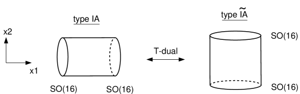
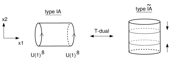
Figure 1: Type IA and $\widetilde{\hbox{\rm\mbox{{\hbox{\cmss IA}}}}}$ compactifications for unbroken $E_{8}\times E_{8}$. There are 8 D8-branes at every orientifold, giving $SO(16)$ gauge symmetry.

Figure 2: Turning on a heterotic Wilson line deforms the Wilson line $B_{2}$ in type IA, breaking $SO(16)$ to $U(1)^{8}$. In type $\widetilde{\hbox{\rm\mbox{{\hbox{\cmss IA}}}}}$ it moves the D8-branes away from the orientifolds.

To construct the heterotic M(atrix) theory which describes this compactification, we start from type I  IA compactified on ${\bf T}^{2}$. This can be described in M(atrix) theory as a 2+1 dimensional $U(N)$ gauge theory with 16 supercharges, compactified on the T-dual torus $\widetilde{{\bf T}}^{2}$ [17]. This theory has a ${\hbox to0.0pt{\cmss Z\hss}\hskip 1.8pt\hbox{\cmss Z}}_{2}$ symmetry, which we mod out by to obtain the untwisted sector of the heterotic M(atrix) theory on ${\bf S}^{1}\times({\bf S}^{1}/{\hbox to0.0pt{\cmss Z\hss}\hskip 1.8pt\hbox{\cmss Z}}_{2})$. A twisted sector, localized at the orbifold fixed points, must then be introduced for gauge anomaly cancellation. Following [9], we carry out this construction in the next two subsections.

2.1 Type I  IA M(atrix) Theory

We begin by reviewing the description of the type I  IA M(atrix) theory on ${\bf T}^{2}$. This is given by a 2+1 dimensional gauge theory with gauge group $U(N)$ and 16 supercharges, compactified on the dual torus $\widetilde{{\bf T}}^{2}$ [17]. The appropriate gauge theory can be obtained by dimensional reduction of ten-dimensional supersymmetric $U(N)$ Yang-Mills theory. Thus the M(atrix) gauge theory has an $Spin(7)_{R}$ R-symmetry, which may be viewed as originating from the reduced seven dimensions.

Our spinor conventions are as follows. We denote $SO(2,1)$ vector indices by $\alpha,\beta=0,1,2$ and $SO(2,1)$ spinor indices by $a,b=1,2$. The (2+1)-dimensional Dirac matrices $\left(\gamma^{\alpha}\right)_{ab}$ are $2\times 2$ purely imaginary matrices:

$$\gamma^{0}=\sigma^{2}=\left(\begin{array}[]{cc}0&-i\\ +i&0\end{array}\right),\hskip 14.22636pt\gamma^{1}=i\sigma^{1}=\left(\begin{array}[]{cc}0&+i\\ +i&0\end{array}\right),\hskip 14.22636pt\gamma^{2}=i\sigma^{3}=\left(\begin{array}[]{cc}+i&0\\ 0&-i\end{array}\right).$$

These obey $\{\gamma^{\alpha},\gamma^{\beta}\}=-2\eta^{\alpha\beta}{\hbox to0.0pt{1\hss}\hskip 1.6pt\hbox{1}}$ with metric $\eta_{\alpha\beta}=(-++)$. We define $\gamma^{\alpha\beta}={1\over 2}[\gamma^{\alpha},\gamma^{\beta}]$. In odd dimensions, there are two inequivalent representations of the Clifford algebra (both of which give identical representations of the Lorentz group). These matrices have been chosen to satisfy $\gamma^{(3)}\equiv i\gamma^{0}\gamma^{1}\gamma^{2}=+{\hbox to0.0pt{1\hss}\hskip 1.6pt\hbox{1}}$. An inequivalent representation of the Clifford algebra is provided by changing the sign of all $\gamma^{\alpha}$. We also introduce a set of real, antisymmetric $Spin(7)_{R}$ Dirac matrices $\left(\gamma^{i}\right)_{AB}$, where $i,j=3,\cdots,9$ are $Spin(7)_{R}$ vector indices and $A,B=1,\cdots,8$ are $Spin(7)_{R}$ spinor indices. These matrices obey $\{\gamma^{i},\gamma^{j}\}=-2\delta^{ij}{\hbox to0.0pt{1\hss}\hskip 1.6pt\hbox{1}}$, and we take them to satisfy $\gamma^{(8)}\equiv\gamma^{3}\cdots\gamma^{9}=+{\hbox to0.0pt{1\hss}\hskip 1.6pt\hbox{1}}$. The ten-dimensional Dirac matrices can then be constructed as a tensor product.

$$\Gamma^{\alpha}=\left[\begin{array}[]{cc}0&\gamma^{\alpha}\otimes{\hbox to0.0pt{1\hss}\hskip 1.6pt\hbox{1}}_{8\times 8}\\ \gamma^{\alpha}\otimes{\hbox to0.0pt{1\hss}\hskip 1.6pt\hbox{1}}_{8\times 8}&0\end{array}\right]\hskip 28.45274pt\Gamma^{i}=\left[\begin{array}[]{cc}0&-i{\hbox to0.0pt{1\hss}\hskip 1.6pt\hbox{1}}_{2\times 2}\otimes\gamma^{i}\\ +i{\hbox to0.0pt{1\hss}\hskip 1.6pt\hbox{1}}_{2\times 2}\otimes\gamma^{i}&0\end{array}\right]$$

This is in a Majorana-Weyl representation, with

$$\Gamma^{(11)}\equiv\Gamma^{0}\cdots\Gamma^{9}=\left[\begin{array}[]{cc}+{\hbox to0.0pt{1\hss}\hskip 1.6pt\hbox{1}}&0\\ 0&-{\hbox to0.0pt{1\hss}\hskip 1.6pt\hbox{1}}\end{array}\right].$$

The field content of the M(atrix) gauge theory is a gauge field $A_{\alpha}$, seven adjoint scalar fields $X_{i}$, and an adjoint spinor field $\psi_{aA}$ satisfying $\Gamma^{(11)}\psi=\psi$. The Lagrangian, obtained by dimensional reduction from (9+1) dimensions, is given by

$$L = -{1\over 2g^{2}_{\scriptscriptstyle YM}}\int_{{\widetilde{T}}_{2}}d^{2}x\,{\rm Tr}\Big{\{}F_{\alpha\beta}F^{\alpha\beta}+2D_{\alpha}X_{i}D^{\alpha}X^{i}-[X_{i},X_{j}][X^{i},X^{j}]$$ (3)

$$\qquad\qquad\qquad\qquad-2i{\overline{\psi}}_{A}\gamma^{\alpha}D_{\alpha}\psi_{A}+2i{\overline{\psi}}_{A}\gamma^{i}_{AB}[X_{i},\psi_{B}]\,\,\Big{\}}$$

where we have suppressed the $SO(2,1)$ spinor indices. This action can be regarded as the world-volume action for a stack of $N$ D2-branes wrapped on ${\widetilde{T}}_{2}$. The gauge coupling is related to the M-theory and type $\widetilde{\hbox{\rm\mbox{{\hbox{\cmss IA}}}}}$ parameters by

$$g^{2}_{\scriptscriptstyle YM} = {2R_{11}\over R_{1}R_{2}}$$ (4)

$$= 2\widetilde{g}_{A}/\sqrt{\alpha^{\prime}_{A}}$$

as can be seen by normalizing the energy of a quantum of electric flux to agree with the energy of a D0-brane Kaluza-Klein mode.

This action is invariant under the ‘dynamical’ supersymmetry transformations

$$\delta_{\epsilon}A_{\alpha} = +{i\over 2}\,{\overline{\epsilon}}_{A}\gamma_{\alpha}\psi_{A}$$

$$\delta_{\epsilon}X^{i} = -{1\over 2}\,{\overline{\epsilon}}_{A}\gamma^{i}_{AB}\psi_{B}$$

$$\delta_{\epsilon}\psi_{A} = -{1\over 4}F_{\alpha\beta}\gamma^{\alpha\beta}\epsilon_{A}-{i\over 2}D_{\alpha}X_{i}\gamma^{\alpha}\gamma^{i}_{AB}\epsilon_{B}-{i\over 4}[X_{i},X_{j}]\gamma^{ij}_{AB}\epsilon_{B}\,.$$ (5)

It is also invariant under the ‘kinematical’ supersymmetry transformations

$$\delta_{\eta}A_{\alpha} = \delta_{\eta}X_{i}=0$$

$$\delta_{\eta}\psi_{A} = \eta_{A}{\hbox to0.0pt{1\hss}\hskip 1.6pt\hbox{1}}.$$ (6)

Note that kinematical supersymmetry acts only on the center-of-mass $U(1)$ part of the $U(N)$ M(atrix) gauge group.

The M-theory origin of these symmetries is easily understood [20]. M-theory has a total of 32 supersymmetries, which decompose into ${\bf 16}_{+}\oplus{\bf 16}_{-}$ of $SO(9,1)$. The choice of infinite momentum frame breaks the supersymmetries in the ${\bf 16}_{-}$, which become the non-linearly realized kinematical supersymmetries of M(atrix) theory. The supersymmetries in the ${\bf 16}_{+}$ are unbroken and give rise to the dynamical supersymmetries of M(atrix) theory. Further decomposing under $SO(2,1)\times SO(7)\subset SO(9,1)$, note that the 2+1-dimensional spinors $\epsilon_{A}$ and $\eta_{A}$ should be taken to be in inequivalent (opposite-sign) representations of the (2+1)-dimensional Clifford algebra.

2.2 Heterotic M(atrix) Theory

The I  IA M(atrix) theory Lagrangian is invariant under a combined ${\hbox to0.0pt{\cmss Z\hss}\hskip 1.8pt\hbox{\cmss Z}}_{2}$ operation $\Omega\cdot P$, where $\Omega$ corresponds to orientation reversal in string theory, and $P$ is a (2+1)-dimensional parity transformation. Orientation reversal acts as

$$\Omega\hskip 14.22636pt:\hskip 14.22636ptA_{\alpha}(x,y) \rightarrow \pm\,A_{\alpha}^{\rm T}(x,y)$$

$$X_{i}(x,y) \rightarrow \pm\,X_{i}^{\rm T}(x,y)$$ (7)

$$\psi_{aA}(x,y) \rightarrow \pm\,\psi_{aA}^{\rm T}(x,y)\,\,.$$

We will only consider the $(-)$ choice of sign in the definition of $\Omega$, for reasons given below. The (2+1)-dimensional parity transformation $P$ acts as

$$P\hskip 14.22636pt:\hskip 14.22636ptA_{0,1}(x,y) \rightarrow +\,A_{0,1}(x,-y)$$

$$A_{2}(x,y) \rightarrow -\,A_{2}(x,-y)$$

$$X_{i}(x,y) \rightarrow -\,X_{i}(x,-y)$$ (8)

$$\psi_{aA}(x,y) \rightarrow +i(\gamma^{2})_{ab}\,\psi_{bA}(x,-y)\,\,.$$

Note that the scalar fields $X_{i}$ are taken to be pseudo-scalar.

As in [9], heterotic M(atrix) theory is obtained from type I  IA M(atrix) theory by modding out by $\Omega\cdot P$. In other words, the heterotic M(atrix) theory is defined as a parameter space orbifold of the I  IA M(atrix) theory. The parity transformation $P$ acts on the parameter space as an involution, so the dual torus $\widetilde{{\bf T}}^{2}$ becomes a dual orbifold with cylinder topology:

$${\widetilde{C}}_{2} = {\bf S}^{1}\times({\bf S}^{1}/{\hbox to0.0pt{\cmss Z\hss}\hskip 1.8pt\hbox{\cmss Z}}_{2})$$

$$x \approx x+2\pi{\widetilde{R}}_{1}$$

$$0 \leq y\,\,\,\leq\,\,\,\pi{\widetilde{R}}_{2}\,\,\,.$$

In addition, at the orbifold fixed circles $y=0$ and $y=\pi{\widetilde{R}}_{2}$, the action of $\Omega\cdot P$ imposes boundary conditions on the fields:

$$(A_{0},\,\,A_{1},\,\,\psi_{2A})(x) {\tt antisymmetric}$$

$$(A_{2},\,\,X^{i},\,\,\psi_{1A})(x) {\tt symmetric}$$

$$\partial_{2}(A_{0},\,\,A_{1},\,\,\psi_{2A})(x) {\tt symmetric}$$

$$\partial_{2}(A_{2},\,\,X^{i},\,\,\psi_{1A})(x) {\tt antisymmetric}\,\,\,.$$ (9)

Note that these conditions imply that $F_{01}$ is antisymmetric on the boundary, while $F_{02}$ and $F_{12}$ are symmetric. In particular, the $U(1)$ part of the electric field in the circle direction vanishes identically on the boundary, which will be important later in establishing S-duality of M(atrix) theory. Heuristically, this may be understood as follows. A propagating photon has an electric field which is orthogonal to its direction of motion. Along the orbifold direction, there is no propagating photon. Consequently, along the circle direction, there is no electric field.

These boundary conditions modify the M(atrix) gauge theory in several ways. First, they break half the supersymmetry. The dynamical supersymmetry parameters $\epsilon_{A}$ appearing in (5) must be taken to be invariant under the ${\hbox to0.0pt{\cmss Z\hss}\hskip 1.8pt\hbox{\cmss Z}}_{2}$ projection, $\epsilon_{A}=i\gamma^{2}\epsilon_{A}$. We will refer to this amount of supersymmetry as ${\cal N}=(0,8)$ supersymmetry in 2+1 dimensions. At the same time, to respect the boundary conditions on the fermions, the kinematical supersymmetry parameters $\eta_{A}$ must satisfy $\eta_{A}=-i\gamma^{2}\eta_{A}$. This sign difference reflects the fact that $\epsilon_{A}$ and $\eta_{A}$ are in inequivalent representations of the (2+1)-dimensional Clifford algebra.

Second, at the boundaries, only gauge transformations in an $O(N)$ subgroup of $U(N)$ are allowed, since a gauge transformation $A_{\alpha}\rightarrow U\left(A_{\alpha}-i\partial_{\alpha}\right)U^{-1}$ respects the boundary conditions only if $U^{\rm T}U|_{y=0,\pi\widetilde{R}_{2}}={\hbox to0.0pt{1\hss}\hskip 1.6pt\hbox{1}}$. Note that under the boundary $O(N)$ gauge group $\{A_{0},A_{1},\psi_{2A}\}$ transform in the adjoint representation, while $\{A_{2},X^{i},\psi_{1A}\}$ are in the symmetric representation.

Finally, but most importantly, the boundary conditions lead to the gauge anomaly discussed in [8, 13]. The fermions $\psi_{A}$ have normalizeable modes which are independent of the coordinate $y$. These modes behave as if they were fermions in 1+1 dimensions. From the 2+1-dimensional Dirac equation, we find that the upper components $\psi_{1A}$ are right-moving, while the lower components $\psi_{2A}$ are left-moving. These modes therefore generate a left-moving $O(N)$ gauge anomaly proportional to $8I_{2}({\tt adj.})-8I_{2}({\tt symm.})=-32I_{2}({\tt fund.})$. Here $I_{2}({\tt R})$ is the quadratic index of the representation ${\tt R}$. An argument given in [5] shows that half of the anomaly must be symmetrically localized on each orbifold boundary.

The anomaly can be cancelled by introducing 32 left-moving Majorana-Weyl fermions in the fundamental representation of $O(N)$. For sufficiently large $N$, this is the unique choice of representation which cancels the anomaly. In order to cancel the anomaly locally, half of these fermions must be localized at each orbifold boundary. They can be regarded as a twisted sector of the M(atrix) theory ${\hbox to0.0pt{\cmss Z\hss}\hskip 1.8pt\hbox{\cmss Z}}_{2}$ orbifold. From the string theory point of view, they can be understood as coming from the 2-8 strings present in type $\widetilde{\hbox{\rm\mbox{{\hbox{\cmss IA}}}}}$ string theory [11].

Note that, had we chosen the $(+)$ sign in the definition of $\Omega$, the boundary gauge group would be $USp(N)$ [8]. In this case, there is no way to cancel the gauge anomaly, since negative numbers of fermions would have to be introduced.

To summarize, the untwisted sector of heterotic M(atrix) theory is described by a (2+1)-dimensional gauge theory on the dual orbifold ${\tilde{C}}_{2}$:

$$L_{\rm untwisted} = -{1\over g^{2}_{\scriptscriptstyle YM}}\int_{{\widetilde{C}}_{2}}d^{2}x\,{\rm Tr}\Big{\{}F_{\alpha\beta}F^{\alpha\beta}+2D_{\alpha}X_{i}D^{\alpha}X^{i}-[X_{i},X_{j}][X^{i},X^{j}]$$ (10)

$$\qquad\qquad\qquad\qquad-2i{\overline{\psi}}_{A}\gamma^{\alpha}D_{\alpha}\psi_{A}+2i{\overline{\psi}}_{A}\gamma^{i}_{AB}[X_{i},\psi_{B}]\,\,\Big{\}}$$

An overall factor of two has been inserted because we write the action only on the fundamental domain of the ${\hbox to0.0pt{\cmss Z\hss}\hskip 1.8pt\hbox{\cmss Z}}_{2}$ action.

The twisted sector involves real chiral fermions $\chi^{(1)}$ and $\chi^{(2)}$ localized at $y=0$ and $\pi\widetilde{R}_{2}$, respectively. They are left-moving, so these fermions are $(0,8)$ supersymmetry singlets. They are in the fundamental representation of the boundary M(atrix) gauge group $O(N)\subset U(N)$, and under the $SO(16)\times SO(16)$ symmetry associated with the 8 D8-branes present at each orientifold, they transform as $({\bf 16},{\bf 1})$ and $({\bf 1},{\bf 16})$, respectively. Their Lagrangian is ($\partial_{\pm}=\partial_{0}\pm\partial_{1}$)

$$L_{\rm twisted} = i\oint dx\,\Big{\{}\,\,\chi^{(1)}\left(\partial_{-}+i\left.A_{-}\right|_{y=0}+iB^{(1)}_{-}\right)\chi^{(1)}$$ (11)

$$\qquad\qquad\!\!\!+\chi^{(2)}\left(\partial_{-}+i\left.A_{-}\right|_{y=\pi\widetilde{R}_{2}}+iB^{(2)}_{-}\right)\chi^{(2)}\,\,\Big{\}}.$$

We have included couplings to the background fields $B^{(1)}$ and $B^{(2)}$, which are the $SO(16)$ gauge fields that propagate on the D8-branes at $y=0$ and $y=\pi\widetilde{R}_{2}$. Recall that the $E_{8}\times E_{8}$ heterotic string corresponds to Wilson lines $\left(B^{(1)},B^{(2)}\right)=\left(0^{8},({\scriptscriptstyle 1\over 2})^{8}\right)$. The (1+1)-dimensional dynamics of the gauge fields $(A_{0},A_{1})$ is not explicitly given but is tacitly assumed to be part of the untwisted sector Lagrangian (10).

The twisted sector does not seem to have a direct derivation from the underlying I  IA M(atrix) theory, and must be introduced by hand (see however [16]). But it is necessary for internal consistency. Note that the boundary conditions on $A_{0}$ and $A_{1}$ force them to be purely imaginary and antisymmetric at the orbifold fixed points, as appropriate for them to couple to the (1+1)-dimensional real chiral fermions located at the boundaries.

3 Turning on Wilson lines

As we discussed in the previous section, the heterotic string compactified on a circle is equivalent to the strong-coupling limit of type IA on an $({\bf S}^{1}/{\hbox to0.0pt{\cmss Z\hss}\hskip 1.8pt\hbox{\cmss Z}}_{2})\times{\bf S}^{1}$ orbifold. Unbroken $E_{8}\times E_{8}$ gauge symmetry corresponds to a symmetric configuration, in which 8 D8-branes (plus their images) are located at each ${\hbox to0.0pt{\cmss Z\hss}\hskip 1.8pt\hbox{\cmss Z}}_{2}$ fixed point and a Wilson line $B_{2}=\left(0^{8},({\scriptscriptstyle 1\over 2})^{8}\right)$ is turned on around the ${\bf S}^{1}$.

We now wish to generalize this, by turning on a Wilson line in the heterotic string. Taking the Wilson line to lie in an $SO(16)\times SO(16)$ subgroup of $E_{8}\times E_{8}$, it is easy to see what this corresponds to in terms of the equivalent type IA theory. The eight coincident D8-branes at each end of the cylinder have a world-volume gauge group $SO(16)\times SO(16)$. Turning on the heterotic Wilson line corresponds to deforming the Wilson line $B_{2}$ in the world-volume theory of these D8-branes.

To describe this in M(atrix) theory, we apply T-duality to both directions of the orbifold $({\bf S}^{1}/{\hbox to0.0pt{\cmss Z\hss}\hskip 1.8pt\hbox{\cmss Z}}_{2})\times{\bf S}^{1}$. This takes us to type $\widetilde{\hbox{\rm\mbox{{\hbox{\cmss IA}}}}}$ theory on the dual orbifold ${\bf S}^{1}\times({\bf S}^{1}/{\hbox to0.0pt{\cmss Z\hss}\hskip 1.8pt\hbox{\cmss Z}}_{2})$. Again, we emphasize that the duality interchanges the orbifold and circle directions, and maps the Wilson line $B_{2}$ in type IA to the positions of the D8-branes along the ${\bf S}^{1}/{\hbox to0.0pt{\cmss Z\hss}\hskip 1.8pt\hbox{\cmss Z}}_{2}$ in type $\widetilde{\hbox{\rm\mbox{{\hbox{\cmss IA}}}}}$. So for unbroken $E_{8}\times E_{8}$, type $\widetilde{\hbox{\rm\mbox{{\hbox{\cmss IA}}}}}$ will have a Wilson line $B_{1}=\left(0^{8},\left({\scriptscriptstyle 1\over 2}\right)^{8}\right)$ turned on and 8 D8-branes located at each orientifold. Turning on a heterotic Wilson line moves the D8-branes away from the type $\widetilde{\hbox{\rm\mbox{{\hbox{\cmss IA}}}}}$ orientifolds, while leaving the $\widetilde{\hbox{\rm\mbox{{\hbox{\cmss IA}}}}}$ Wilson line $B_{1}$ unchanged. See Figs. 1 and 2.

The D8-branes give rise to chiral fermions in the M(atrix) theory, which can be thought of as 2-8 strings in type $\widetilde{\hbox{\rm\mbox{{\hbox{\cmss IA}}}}}$ string theory. When the 8-branes move away from the ends of the cylinder, these 2-8 strings will move with them. So we expect that the M(atrix) theory description of the heterotic string with a Wilson line will involve a (2+1)-dimensional Yang-Mills theory on ${\bf S}^{1}\times({\bf S}^{1}/{\hbox to0.0pt{\cmss Z\hss}\hskip 1.8pt\hbox{\cmss Z}}_{2})$, coupled to 16 complex chiral fermions $\chi_{I}$ which propagate on circles at fixed positions $y=y_{I}$, $I=1,\ldots,16$ along the orbifold direction.

This raises an interesting puzzle. From the spacetime point of view, the D8-branes are sources of R-R and NS-NS fields. Tadpoles from disc diagrams localized near the D8-branes produce a flux that is absorbed by ${\hbox{\cmss R}\hbox to0.0pt{\hss\vrule height=7.1pt,width=0.4pt,depth=-0.1pt\hskip 0.6pt\phantom{.}}}{\hbox{\cmss P}\hbox to0.0pt{\hss\vrule height=7.1pt,width=0.4pt,depth=-0.1pt\hskip 0.6pt\phantom{.}}}^{2}$ diagrams localized near the orientifolds. When the D8-branes are symmetrically distributed at the ends of the cylinder, this tadpole cancellation takes place locally, and the spacetime fields in the bulk of the cylinder are constant. But when the D8-branes move away from the type $\widetilde{\hbox{\rm\mbox{{\hbox{\cmss IA}}}}}$ orbifold boundaries, they create a flux along the axis of the cylinder. The resulting R-R and NS-NS fields were found in [6] by solving spacetime equations of motion. How does the M(atrix) gauge theory reproduce this physics?

A key observation is that the formulation of the M(atrix) theory we sketched above cannot be the complete story — it has a gauge anomaly. The fermions $\psi_{A}$ have modes, constant along the orbifold direction, which are chiral in the (1+1)-dimensional sense. These modes give rise to a gauge anomaly, which is symmetrically distributed between the two ends of the cylinder. The fermions $\chi_{I}$, which can be thought of as 2-8 strings, had to be introduced to cancel the anomaly. When these fermions are symmetrically distributed between the two ends of the cylinder the anomaly cancellation is local. But when the D8-branes move away from the boundaries of the $\widetilde{\hbox{\rm\mbox{{\hbox{\cmss IA}}}}}$ orbifold, the $\chi_{I}$ fermions move with them, and anomaly cancellation is possible only if there is an additional interaction present in the M(atrix) gauge theory which can ‘move the anomaly’ from the positions of the D8-branes to the ends of the cylinder.

This leads us to state that the correct formulation of M(atrix) theory in the presence of a Wilson line is to be found by enforcing internal consistency conditions on the (2+1)-dimensional Yang-Mills theory, namely cancellation of gauge and supersymmetry anomalies. For the ${\bf S}^{1}$ compactification that we are considering, this is sufficient to uniquely determine the M(atrix) theory Lagrangian, at least through two-derivative order. As we shall see, an internally consistent (2+1)-dimensional action will automatically correctly take into account both the R-R and NS-NS background fields produced by the D8-branes. It achieves this by explicitly breaking (2+1)-dimensional Poincaré invariance.

This provides an interesting variation on the idea of D-branes as probes of background geometry [24, 25, 26, 27]. The configurations studied previously have involved systems of parallel branes, so the field theory living on the probe is Poincaré invariant. Typically the probe theory has a flat classical moduli space. But one finds that quantum corrections to the moduli space metric precisely encode the non-trivial spacetime geometry that is established by the other branes.

In the system we are considering, which can be thought of as an intersecting 2-brane – 8-brane system in type I  IA, it is likewise true that the field theory on the probe 2-brane knows about the background geometry due to the 8-brane. But it is now encoded into (non-Poincaré-invariant) terms which must be added to the classical probe action, in order to obtain a consistent (supersymmetric and anomaly-free) probe theory.

3.1 Gauge Anomaly Cancellation

When a heterotic Wilson line is turned on, the D8-branes of type $\widetilde{\hbox{\rm\mbox{{\hbox{\cmss IA}}}}}$ move away from the orbifold boundaries, to positions $y=y_{I}$, $I=1,\ldots,16$ along the orbifold direction. So we expect the M(atrix) theory to include 16 (1+1)-dimensional complex chiral fermions $\chi_{I}$, which can be thought of as unexcited 2-8 strings, localized at positions $y_{I}$ in the bulk of the orbifold.

These chiral fermions are in the fundamental representation of the M(atrix) theory $U(N)$ gauge group, and should couple in the usual way ($\partial_{\pm}=\partial_{0}\pm\partial_{1}$).

$$S_{\chi}=i\int d^{3}x\sum_{I=1}^{16}\delta(y-y_{I})\overline{\chi}_{I}\left(\partial_{-}+iA_{-}+iB_{-}^{(I)}\right)\chi_{I}$$ (12)

Here $A$ is the $U(N)$ gauge field, and $B^{(I)}$ is the $U(1)$ gauge field on the $I^{th}$ D8-brane. The effective action $\Gamma_{I}[A]$ obtained by integrating out the the field $\chi_{I}$ is not gauge invariant. Rather, it has an anomalous variation under gauge transformations $\delta_{\Lambda}A=d\Lambda+i[A,\Lambda]$.

$$\delta_{\Lambda}\Gamma_{I}=-{1\over 4\pi}I_{2}({\tt fund.})\int{\rm Tr}\left.\left(\Lambda dA\right)\right|_{y=y_{I}}$$ (13)

There is no gauge anomaly in odd dimensions, so the (2+1) dimensional Yang-Mills theory must be anomaly-free in the bulk of the dual orbifold. But, as we discussed in the previous section, the fermions $\psi_{A}$ have normalizeable modes which are independent of $y$. One can think of these modes as if they were fermions in 1+1 dimensions. The upper component $\psi_{1A}$ is a right-moving symmetric tensor, while the lower component $\psi_{2A}$ is a left-moving adjoint. So integrating out these modes induces an effective action $\Gamma_{\psi}$ with a gauge anomaly. As in [5], the anomaly must be a sum of two terms. Each term is localized at one end of the cylinder, and has half the strength of the standard 1+1 dimensional anomaly. Compared to $\Gamma_{I}$, an additional factor of $1/2$ arises because the fermions $\psi_{A}$ are real instead of complex.

$$\delta_{\Lambda}\Gamma_{\psi} = -{1\over 16\pi}\left(8I_{2}({\tt adj.})-8I_{2}({\tt symm.})\right)\int{\rm Tr}\left\{\Lambda dA|_{y=0}+\Lambda dA|_{y=\pi\widetilde{R}_{2}}\right\}$$ (14)

$$= 8\,{1\over 4\pi}I_{2}({\tt fund.})\int{\rm Tr}\left\{\Lambda dA|_{y=0}+\Lambda dA|_{y=\pi\widetilde{R}_{2}}\right\}$$

Here $I_{2}({\tt adj.})=N-2$ and $I_{2}({\tt symm.})=N+2$ are the quadratic indices of the adjoint and symmetric representation of $O(N)\subset U(N)$, normalized so that $I_{2}({\tt fund.})=1$.

To have a gauge-invariant theory we must add a term to the classical action which is not gauge invariant, but whose gauge variation will cancel these anomalies due to the fermions. Consider adding a Chern-Simons term to the action:

$$S=\int d^{3}x\,\nu(y)\epsilon^{\alpha\beta\gamma}{\rm Tr}\bigl{(}A_{\alpha}\partial_{\beta}A_{\gamma}+i{2\over 3}A_{\alpha}A_{\beta}A_{\gamma}\bigr{)}\,\,\,.$$

The Chern-Simons coupling $\nu(y)$ is taken to be piecewise constant between the 8-branes, but with a discontinuity at the location of every 8-brane:

$$\nu(y)=\nu_{0}\left(-8+\sum_{I=1}^{16}\theta(y-y_{I})\right)\,\,\,.$$ (15)

Under a gauge transformation the Chern-Simons action has an anomalous variation

$$\delta_{\Lambda}S=\int\nu(y)\,d\,{\rm Tr}(\Lambda dA)\,.$$

Integration by parts turns this into a sum of localized contributions:

$$\delta_{\Lambda}S=\int{\rm Tr}\left(8\nu_{0}(\Lambda dA)|_{y=0}+8\nu_{0}(\Lambda dA)|_{y=\pi\widetilde{R}_{2}}-\nu_{0}\sum_{I=1}^{16}(\Lambda dA)|_{y=y_{I}}\right)\,\,\,.$$

So including the Chern-Simons term will cancel the fermion anomalies, provided we choose the coefficient $\nu_{0}=-1/4\pi$.

The presence of the Chern-Simons term follows purely from anomaly considerations in 2+1 dimensions, but it also has a clear spacetime origin and interpretation, which we now outline. From the spacetime point of view the D8-branes are sources for the R-R 10-form field strength, which plays the role of a cosmological constant in massive I  IA supergravity [28, 29]. The 10-form field strength is piecewise constant between the 8-branes, but jumps at the location of an 8-brane [6]. This is exactly the behavior of the function $\nu(y)$, which suggests that we should identify $\nu(y)$ with the (dual of) the R-R 10-form field strength.

This identification can be made precise by noting that the R-R 10-form indeed couples to a 2-brane via a Chern-Simons term [30]. This coupling can be heuristically motivated by expanding the coupling between the R-R $(p+1)$-form potentials $C^{(p+1)}$ and the 2-brane world-volume field strength $F$ [31, 32, 33], and integrating by parts:

$$S = \int C\,{\rm Tr}\,e^{F}$$

$$= \int C^{(3)}+C^{(1)}{\rm Tr}(F)+{1\over 2}C^{(-1)}{\rm Tr}\left(F^{2}\right)$$

$$= \int\cdots+{1\over 2}dC^{(-1)}{\rm Tr}\left(AdA+i{2\over 3}A^{3}\right)$$

We can formally regard $dC^{(-1)}$ as the dual of the 10-form field strength, and identify it with $\nu(y)$. This provides the spacetime derivation of the Chern-Simons coupling we found above from world-volume gauge theory considerations.

3.2 Supersymmetry Anomaly Cancellation

The next step is to build a supersymmetric action which incorporates the Chern-Simons term. The Chern-Simons term by itself breaks supersymmetry, and to restore it we will have to modify the rest of the M(atrix) theory action in an appropriate way. The spacetime interpretation of this procedure is clear: turning on the Chern-Simons term is equivalent to turning on a R-R background, which breaks supersymmetry unless an appropriate NS-NS background is also turned on. The reader who does not wish to see the details can skip ahead to the next sub-section, where we give the results in components.

Let us first outline what we expect to find. In the infinite momentum frame, the 32 supersymmetries of M-theory are organized into 16 dynamical supersymmetries that act linearly on the fields, and 16 kinematical supersymmetries that are non-linearly realized [20]. The heterotic compactification on $({\bf S}^{1}/{\hbox to0.0pt{\cmss Z\hss}\hskip 1.8pt\hbox{\cmss Z}}_{2})\times{\bf S}^{1}$ breaks half the supersymmetry, so we expect to find 8 dynamical and 8 kinematical supersymmetries in the M(atrix) theory.

In this section we will be primarily concerned with achieving dynamical supersymmetry. In 2+1 dimensions, in terms of eight spinor supercharges $\hbox{\cmss Q}_{A=1,\ldots,8}$, the dynamical supersymmetries are generated by $\bar{\epsilon}_{A}\hbox{\cmss Q}_{A}$, where the $\epsilon_{A}$ are eight spinor parameters invariant under the orbifold ${\hbox to0.0pt{\cmss Z\hss}\hskip 1.8pt\hbox{\cmss Z}}_{2}$ action, $i\gamma^{2}\epsilon_{A}=\epsilon_{A}$. We will refer to this amount of supersymmetry as ${\cal N}=(0,8)$ in 2+1 dimensions.

Note that ${\cal N}=(0,8)$ supersymmetry does not require (2+1)-dimensional Poincaré invariance: the supersymmetry algebra closes on translations in the $t$ and $x$ directions, but does not include translations in the orbifold direction $y$. We do, however, expect the system to have a $Spin(7)$ R-symmetry, corresponding to spatial rotations in the directions orthogonal to the 2-brane.

We will work in terms of ${\cal N}=1$ superfields in 2+1 dimensions (see Appendix A). This will only allow us to make a $G_{2}$ subgroup of $Spin(7)_{R}$ manifest. We introduce a vector multiplet

$$\Gamma_{a}=iA_{\alpha}\left(\gamma^{\alpha}\theta\right)_{a}+{\bar{\theta}\theta}\lambda_{a}$$

and seven adjoint scalar multiplets

$$\Phi_{i}=X_{i}+\bar{\theta}\psi_{i}+{1\over 2}{\bar{\theta}\theta}F_{i}$$

where $i=1,\ldots,7$ is an index in the ${\bf 7}$ of $G_{2}$. Also $a=1,2$ is an $SO(2,1)$ spinor index, while $\alpha=0,1,2$ is an $SO(2,1)$ vector index. The hallmark of ${\cal N}=(0,8)$ supersymmetry will be the appearance of an enhanced $Spin(7)_{R}$ symmetry, under which the seven scalars $X_{i}$ transform as a vector and the eight fermions $\lambda,\psi_{i}$ transform as a spinor.

Our starting point is the fact that the usual (Poincaré invariant) ${\cal N}=8$ Yang-Mills Lagrangian is the ${\bar{\theta}\theta}$ component of

$${\cal F}={\rm Tr}\,\left({1\over 2}W^{a}W_{a}-2\nabla^{a}\Phi_{i}\nabla_{a}\Phi_{i}+f_{ijk}\Phi_{i}[\Phi_{j},\Phi_{k}]\right)$$

where $f_{ijk}$ is a suitably normalized totally antisymmetric $G_{2}$-invariant tensor. This leads us to expect a term in the action

$$S=-{1\over\bar{g}^{2}_{\scriptscriptstyle YM}}\int d^{3}x\,z(y){\cal F}|_{{\bar{\theta}\theta}}\,.$$

Since we do not expect to have translation invariance along the axis of the cylinder, we have allowed for the possibility that the coupling constant depends on $y$ through some unknown function $z(y)$. In the central region where the cosmological constant $\nu(y)$ vanishes, we will choose to normalize $z(y)=1$.

As it stands this action is not supersymmetric. Under a supersymmetry variation the ${\bar{\theta}\theta}$ component of ${\cal F}$ changes by a total derivative, which can then act on $z(y)$. There is a simple way to modify any action of this form to restore at least ${\cal N}=(0,1)$ supersymmetry. Consider the component expansion of ${\cal F}$:

$${\cal F}=A+\bar{\theta}\xi+{\bar{\theta}\theta}L\,\,\,.$$

Under supersymmetry the top component of ${\cal F}$ changes by a total divergence, $\delta_{\epsilon}L=-{i\over 2}\bar{\epsilon}\gamma^{\alpha}\partial_{\alpha}\xi$. So the action built just from $L$ has a supersymmetry variation (after integrating by parts)

$$\delta_{\epsilon}S = -{1\over\bar{g}^{2}_{\scriptscriptstyle YM}}\int d^{3}x\,{dz\over dy}{i\over 2}\bar{\epsilon}\gamma^{2}\xi$$

$$= -{1\over\bar{g}^{2}_{\scriptscriptstyle YM}}\int d^{3}x\,{dz\over dy}\left(-{1\over 2}\right)\bar{\epsilon}\xi\,\,\,.$$

In the second line we used the fact that the spinor parameter $\epsilon$ satisfies the orbifold projection condition $i\gamma^{2}\epsilon=\epsilon$. But now, noting that the supersymmetry variation of the bottom component of ${\cal F}$ is $\delta_{\epsilon}A=\bar{\epsilon}\xi$, we see that we can compensate for the supersymmetry variation of this action by adding a term to the Lagrangian proportional to the bottom component of ${\cal F}$. This leads us to the ${\cal N}=(0,1)$ supersymmetric Yang-Mills action

$$S_{YM}=-{1\over\bar{g}^{2}_{\scriptscriptstyle YM}}\int d^{3}x\,\left(z(y){\cal F}|_{{\bar{\theta}\theta}}+{1\over 2}{dz\over dy}{\cal F}|_{\theta=0}\right)\,.$$

This will be one term in our M(atrix) gauge theory action.

Unfortunately, adding the bottom component of ${\cal F}$ to the Lagrangian breaks the $Spin(7)$ R-symmetry we were hoping to achieve. To see this, note that the bottom component of ${\cal F}$ has a term involving the tensor $f_{ijk}$.

$${\cal F}|_{\theta=0}={\rm Tr}\left(2\overline{\lambda}\lambda-2\overline{\psi}_{i}\psi_{i}+f_{ijk}X_{i}[X_{j},X_{k}]\right)$$

$f_{ijk}$ is invariant under $G_{2}$, but not invariant under $Spin(7)_{R}$, so this term must be canceled.

This can be done by introducing a superpotential. From ${\cal W}={\rm Tr}\,\left(\Phi_{i}\Phi_{i}\right)$ we build a $(0,1)$ supersymmetric action:

$$S_{W}=-{1\over\bar{g}^{2}_{\scriptscriptstyle YM}}\int d^{3}x\,\left(-{4\over 3}{dz\over dy}{\cal W}|_{{\bar{\theta}\theta}}-{2\over 3}{d^{2}z\over dy^{2}}{\cal W}|_{\theta=0}\right)\,\,\,.$$

The sum $S_{YM}+S_{W}$ has a $Spin(7)_{R}$-invariant potential for the bosonic fields. To make this manifest one must eliminate the auxiliary fields using their equations of motion.

$$F_{i}={3\over 8}f_{ijk}[X_{j},X_{k}]-{1\over 3z}{dz\over dy}X_{i}$$

The cross term from $|F_{i}|^{2}$ cancels against the unwanted term $f_{ijk}X_{i}[X_{j},X_{k}]$ which appeared in ${\cal F}|_{\theta=0}$.

We have not yet achieved a $Spin(7)_{R}$ symmetry which includes the fermions. To see this the relevant terms in the action are

$$S_{YM}+S_{W} = -{1\over\bar{g}^{2}_{\scriptscriptstyle YM}}\int d^{3}x\,{\rm Tr}\biggl{\{}z(y)\left(-2i\overline{\lambda}\gamma^{\alpha}D_{\alpha}\lambda-2i\overline{\psi}_{i}\gamma^{\alpha}D_{\alpha}\psi_{i}\right)$$ (16)

$$\qquad\qquad\qquad\qquad+{dz\over dy}\,\left(\overline{\lambda}\lambda-{1\over 3}\overline{\psi}_{i}\psi_{i}\right)+\cdots\biggr{\}}$$

which arise from the fermion kinetic terms, the bottom component of ${\cal F}$, and the top component of ${\cal W}$. The fermion kinetic terms have a $Spin(7)_{R}$ R-symmetry, but this does not extend to the rest of the action.

This can be fixed by introducing a Chern-Simons term. The Chern-Simons term appears in the top component of a superfield ${\cal G}$ which is given in Appendix A. We introduce the action

$$S_{CS} = \int d^{3}x\,\nu(y){\cal G}|_{{\bar{\theta}\theta}}$$

$$= \int d^{3}x\,\nu(y){\rm Tr}\left\{\epsilon^{\alpha\beta\gamma}\,\left(A_{\alpha}\partial_{\beta}A_{\gamma}+i{2\over 3}A_{\alpha}A_{\beta}A_{\gamma}\right)+\overline{\lambda}\lambda\right\}\,\,\,.$$

The Chern-Simons coupling $\nu(y)$ was determined in the previous section from gauge anomaly cancellation.

$$\nu(y)=-{1\over 4\pi}\left(-8+\sum_{I=1}^{16}\theta(y-y_{I})\right)\,\,\,.$$

If we add the Chern-Simons action to the action (16), the result will be a $Spin(7)_{R}$-invariant potential for the fermions, provided that

$$\nu(y)={4\over 3\bar{g}^{2}_{\scriptscriptstyle YM}}{dz\over dy}\,\,\,.$$ (17)

With this choice, the action $S_{YM}+S_{W}+S_{CS}$ has a $Spin(7)$ R-symmetry. We will be able to make this manifest in the next section when we write the action out in components.

But the Chern-Simons action $S_{CS}$ is not supersymmetric, because the top component of the superfield ${\cal G}$ changes by a total derivative under supersymmetry transformation

$$\delta_{\epsilon}S_{CS}=\int d^{3}x\,\nu(y)\partial_{\alpha}\left[-i\epsilon^{\alpha\beta\gamma}{\rm Tr}\,\left(\bar{\epsilon}\gamma_{\beta}\lambda A_{\gamma}\right)\right]\,\,\,.$$

Integration by parts turns this into a sum of contributions localized at the positions of the D8-branes, plus surface terms at the ends of the cylinder. For spinors satisfying $i\gamma^{2}\epsilon=\epsilon$ the result can be expressed as

$$\delta_{\epsilon}S_{CS}=\int d^{2}x\,\left(8\,{1\over 8\pi}{\rm Tr}\left(A_{-}\delta_{\epsilon}A_{+}\right)|_{y=0,\pi{\scriptstyle\tilde{R}_{2}}}-{1\over 8\pi}\sum_{I=1}^{16}{\rm Tr}\left(A_{-}\delta_{\epsilon}A_{+}\right)|_{y=y_{I}}\right)\,\,\,.$$

The trick we used before to restore supersymmetry, namely adding the bottom component of the superfield ${\cal G}$ to the action, does not work for the Chern-Simons term — the bottom component is not gauge invariant (indeed it vanishes in Wess-Zumino gauge).

What saves us are the chiral fermions $\chi_{I}$ which propagate at the locations of the D8-branes. The fields $\chi_{I}$ are supersymmetry singlets. Their classical action (12) only depends on $A_{-}$, so naively they only couple to the $A_{-}$ component of the gauge field, which is also a singlet under $(0,8)$ supersymmetry. But the effective action $\Gamma_{I}[A_{+},A_{-}]$ obtained by integrating out $\chi_{I}$ is not just a functional of $A_{-}$. Instead, it must be defined to include a local contact term which couples $A_{+}$ to $A_{-}$ [34]. This is a consequence of the anomaly (13), which can be expressed in the equivalent form

$$D_{-}{\delta\Gamma_{I}\over\delta A_{-}}+D_{+}{\delta\Gamma_{I}\over\delta A_{+}}={1\over 8\pi}\left(\partial_{-}A_{+}-\partial_{+}A_{-}\right).$$

This equation can only be satisfied if $\Gamma_{I}$ is defined to include a contact term,

$$\Gamma_{I}[A_{+},A_{-}]={1\over 8\pi}\int d^{2}x\,{\rm Tr}\left(A_{+}A_{-}\right)+\widetilde{\Gamma}_{I}[A_{-}]$$ (18)

where $\widetilde{\Gamma}_{I}$ is an arbitrary functional of $A_{-}$. From this we see that $\Gamma_{I}$ has an anomalous variation under supersymmetry:

$$\delta_{\epsilon}\Gamma_{I}={1\over 8\pi}\int d^{2}x\,{\rm Tr}\left(A_{-}\delta_{\epsilon}A_{+}\right)|_{y=y_{I}}\,\,\,.$$

This is precisely what is needed to cancel the supersymmetry variation of the Chern-Simons term at the location of the D8-branes. A similar supersymmetry anomaly arises from the $y$-independent modes of the fields $\psi_{A}$, as required by their gauge anomaly (14). This will cancel against the surface terms which appeared at the boundaries of the $\widetilde{\hbox{\rm\mbox{{\hbox{\cmss IA}}}}}$ orbifold in the supersymmetry variation of the Chern-Simons term.

The action we have determined, $S_{YM}+S_{W}+S_{CS}+S_{\chi}$, is both supersymmetric and $Spin(7)_{R}$-invariant. It must, therefore, have the desired ${\cal N}=(0,8)$ supersymmetry. In the next section we write out the full action and its $(0,8)$ supersymmetry transformations in components.

3.3 Component Expansion of the M(atrix) Action

In the previous sections we constructed a gauge invariant ${\cal N}=(0,8)$ supersymmetric action. We now collect our results, and expand the action in components. This will allow us to write it in a way that makes the $Spin(7)_{R}$ R-symmetry manifest.

In obtaining the action we were led to introduce two functions

$$\nu(y) = -{1\over 4\pi}\left(-8+\sum_{I=1}^{16}\theta(y-y_{I})\right)$$

$$z(y) = {\rm const.}-{3\bar{g}^{2}_{\scriptscriptstyle YM}\over 32\pi}\sum_{I=1}^{16}\left|y-y_{I}\right|,$$

where the $y_{I}$ are the positions of the D8-branes in type $\widetilde{\hbox{\rm\mbox{{\hbox{\cmss IA}}}}}$. The constant is to be chosen so that $z(y)=1$ in the central region where $\nu(y)=0$.

We emphasize that we have determined these functions by demanding supersymmetry and gauge anomaly cancellation in 2+1 dimensions. But they do have a clear spacetime interpretation: they correspond to the background fields established by the D8-branes. As one might expect, $z(y)$ gives the spatial variation of the NS-NS fields, just as $\nu(y)$ was shown to give the variation of the R-R 10-form in section 3.1. The precise identification comes from noting that in a system of parallel D8-branes the background fields vary according to [6]

$$\begin{array}[]{ll}\hbox{\rm dilaton}&\enskip e^{\phi}\sim z^{-5/6}(y)\\ \vskip 8.5359pt\cr\hbox{\rm metric}&\enskip G_{\mu\nu}\sim z^{-1/3}(y)\,\eta_{\mu\nu}\\ \vskip 8.5359pt\cr\hbox{\rm R-R 10-form}&\enskip F^{(10)}\sim\nu(y)\,dx^{0}\cdots dx^{9}.\end{array}$$

Under $Spin(7)_{R}$, the seven scalars $X_{i}$ transform as a vector, while the eight fermions $\lambda$, $\psi_{i}$ transform as a spinor. At this point it is useful to make a field redefinition. We define

$$Y^{i} = z^{1/3}(y)X_{i}$$

$$\Psi_{A} = \left\{z^{1/3}(y)\lambda,\,\,z^{1/3}(y)\psi_{i}\right\}\,\,.$$

¿From the M(atrix) gauge theory point of view these redefinitions can be motivated by noting that certain properties of the action – the existence of flat directions, as well as kinematical supersymmetry – look most natural in terms of the rescaled variables.

These redefinitions can also be given a simple spacetime motivation. Within the M(atrix) gauge theory the $Spin(7)_{R}$ vector indices $i,j$ are of course raised and lowered with the flat metric $\delta_{ij}$. But from the spacetime point of view it is natural to regard the scalars $X$ as having covariant indices. This is because in constructing a supersymmetric Yang-Mills theory these scalars arise from dimensional reduction of a one-form. But the embedding coordinates for a membrane $Y$ should have contravariant indices. So they are related by a factor of the inverse metric, $Y^{i}=z^{1/3}(y)X_{i}$.

Collecting our results of the previous two sections, expanding in components, and integrating out the auxiliary fields, we find the M(atrix) model action

$$S = -{1\over\bar{g}^{2}_{\scriptscriptstyle YM}}\int d^{3}x\,{\rm Tr}\bigg{\{}z(y)F_{\alpha\beta}F^{\alpha\beta}+2z^{1/3}(y)D_{\alpha}Y_{i}D^{\alpha}Y^{i}-z^{-1/3}(y)[Y_{i},Y_{j}][Y^{i},Y^{j}]$$

$$\quad\qquad\qquad\qquad-2iz^{1/3}(y)\overline{\Psi}_{A}\gamma^{\alpha}D_{\alpha}\Psi_{A}-{dz^{1/3}\over dy}\overline{\Psi}_{A}\Psi_{A}+2i\overline{\Psi}_{A}\gamma^{i}_{AB}[Y_{i},\Psi_{B}]$$

$$\quad\qquad\qquad\qquad-{4\over 3}{dz\over dy}\epsilon^{\alpha\beta\gamma}\bigl{(}A_{\alpha}\partial_{\beta}A_{\gamma}+i{2\over 3}A_{\alpha}A_{\beta}A_{\gamma}\bigr{)}\bigg{\}}$$

$$+i\sum_{I=1}^{16}\int d^{3}x\delta(y-y_{I})\overline{\chi}_{I}\left(\partial_{-}+iA_{-}+iB_{-}^{(I)}\right)\chi_{I}\,\,\,.$$

Here $A_{\alpha}$ is a $U(N)$ gauge field, coupled to adjoint scalars $Y^{i}$ and adjoint fermions $\Psi_{A}$. The fields $\chi_{I}$ are the twisted sector fermions, complex chiral fermions in the fundamental representation of $U(N)$. The field $\chi_{I}$ is also charged under the $U(1)$ gauge field $B^{(I)}$ which propagates on the $I^{th}$ D8-brane.

This action has several symmetries, all of which are necessary for a sensible M(atrix) theory interpretation. As discussed in section 3.1, the gauge anomalies cancel, and the action enjoys a $U(N)$ gauge invariance. Also, as shown in section 3.2, the action is invariant under the ${\cal N}=(0,8)$ dynamical supersymmetry transformation

$$\delta_{\epsilon}A_{\alpha} = {i\over 2}z^{-1/3}(y)\bar{\epsilon}_{A}\gamma_{\alpha}\Psi_{A}$$

$$\delta_{\epsilon}Y^{i} = -{1\over 2}\bar{\epsilon}_{A}\gamma^{i}_{AB}\Psi_{B}$$

$$\delta_{\epsilon}\Psi_{A} = -{1\over 4}z^{1/3}(y)F_{\alpha\beta}\gamma^{\alpha\beta}\epsilon_{A}-{i\over 2}D_{\alpha}Y_{i}\gamma^{\alpha}\gamma^{i}_{AB}\epsilon_{B}-{i\over 4}z^{-1/3}(y)[Y_{i},Y_{j}]\gamma^{ij}_{AB}\epsilon_{B}$$ (20)

$$\delta_{\epsilon}\chi_{I} = 0$$

where the spinor parameter satisfies the ${\hbox to0.0pt{\cmss Z\hss}\hskip 1.8pt\hbox{\cmss Z}}_{2}$ projection condition $\epsilon_{A}=i\gamma^{2}\epsilon_{A}$. There is an associated $Spin(7)$ R-symmetry, which corresponds to spatial rotations in the directions orthogonal to the 2-branes.

The action is also invariant under the ${\cal N}=(0,8)$ kinematical supersymmetry

$$\delta_{\eta}\Psi_{A}=\eta_{A}{\hbox to0.0pt{1\hss}\hskip 1.6pt\hbox{1}}$$ (21)

where the spinor parameter satisfies $\eta_{A}=-i\gamma^{2}\eta_{A}$, and all other variations vanish. Kinematical supersymmetry was discussed in the context of type I  IA matrix theory in section 2.1. It corresponds to those spacetime supersymmetries which are broken (non-linearly realized) due to the choice of infinite momentum frame [20]. As such, it should also hold in heterotic M(atrix) theory. This is easily verified, but note that there is a non-trivial cancellation between the variations of the fermion mass and kinetic terms. Since kinematical supersymmetry did not play a role in our construction of this action, it could be regarded as an accidental symmetry, but one that is necessary to have a sensible M(atrix) theory interpretation.

Finally, the action is invariant under transverse translations

$$Y_{i}\rightarrow Y_{i}+c_{i}{\hbox to0.0pt{1\hss}\hskip 1.6pt\hbox{1}}\,\,.$$

This is simply a spatial translation in the directions orthogonal to the 2-branes. A related observation is that the action has the flat directions required for M(atrix) theory: there are low energy configurations in which the matrices $Y_{i}$ are diagonal, corresponding to widely separated 2-branes. Again, note that this property did not play a role in our construction of the action.

4 BPS States and T-duality

Having established the structure of heterotic M(atrix) theory, we now analyze its BPS excitations, and compare them to the heterotic string. We do this for several reasons. Showing that the BPS spectra agree gives evidence that the M(atrix) theory we have described really does provide a non-perturbative definition of the heterotic string. Also, by matching the BPS spectra, we can relate the parameters of M(atrix) theory to the parameters of the heterotic string. And finally, this will show that heterotic T-duality is realized in M(atrix) theory as a novel form of electric–magnetic S-duality.

The heterotic compactification of M-theory on $\left({\bf S}^{1}/{\hbox to0.0pt{\cmss Z\hss}\hskip 1.8pt\hbox{\cmss Z}}_{2}\right)\times{\bf S}^{1}$ gives rise to a richer spectrum of BPS states than toroidal compactification. This is due to the existence of a twisted sector. Besides the closed membranes of the untwisted sector, there are membranes with boundaries at the orbifold fixed points. These so-called twisted membranes correspond to the charged excitations present in type IA and heterotic string theory.

For future reference, we list the BPS excitations of the heterotic string, and their corresponding states in M-theory and M(atrix) theory. Recall that M-theory is compactified on $\left({\bf S}^{1}/{\hbox to0.0pt{\cmss Z\hss}\hskip 1.8pt\hbox{\cmss Z}}_{2}\right)\times{\bf S}^{1}$, where $x=x^{1}$ is the orbifold direction and $y=x^{2}$ is the circle direction (note that these directions are interchanged in M(atrix) theory). The $x^{11}$ direction along which M-theory is boosted is compactified on a regulator circle of radius $R_{11}$. All the states we discuss are assumed to have momentum $p_{11}=N/R_{11}$ around the regulator circle.

1. winding mode excitations
   A heterotic string wound on ${\bf S}^{1}$ is realized in M-theory as an untwisted membrane wrapped on $x^{1}$-$x^{2}$. In the M(atrix) gauge theory this is realized as a quantum of magnetic flux ${\bf B}$.

2. momentum mode excitations
   A heterotic string with momentum around ${\bf S}^{1}$ is realized as an M-theory graviton with momentum around the $x^{2}$ circle direction. In M(atrix) theory it corresponds to a quantum of electric flux ${\bf E}_{2}$ in the $y$ orbifold direction.

3. charged excitations
   Charged heterotic strings correspond to twisted membranes in M-theory. In M(atrix) theory they arise as excitations of the twisted sector fermions $\chi_{I}$.

4. winding modes on $x^{11}$
   The regulator circle is one of the spatial directions in the heterotic string. A heterotic string wound on this circle corresponds to a longitudinal membrane in M-theory, wrapped on $x^{1}$-$x^{11}$. In M(atrix) theory this corresponds to a photon propagating around the $x$ circle direction.

The first three types are the basic BPS states of interest to us. They can be combined to form additional BPS states, namely charged winding states and charged Kaluza-Klein states. The fourth type of BPS state becomes infinitely heavy as $R_{11}\rightarrow\infty$, but will be useful later for normalizing the M(atrix) theory parameters.

4.1 BPS States for Unbroken $E_{8}\times E_{8}$

We proceed to analyze the BPS states in M(atrix) theory. In this subsection we assume that $E_{8}\times E_{8}$ is unbroken. Recall that in M(atrix) theory this corresponds to a configuration in which a background Wilson line $B_{1}=\left(0^{8},({\scriptscriptstyle 1\over 2})^{8}\right)$ is turned on and 8 twisted sector fermions $\chi_{I}$ are located at each orbifold boundary. We discuss three topics in turn: flux quantization, the BPS conditions and equations of motion, and the spectrum of BPS states.

4.1.1 Flux Quantization

In this section we discuss the allowed $U(N)$ bundles in M(atrix) theory, and the corresponding quantization conditions on electric and magnetic flux.

We begin by constructing the general $U(N)$ bundle on ${\bf T}^{2}$. To describe this, we introduce the $U(N)$ matrix

$$V(y)=\left(\begin{array}[]{cccccc}0&1&&&&\\ &0&1&&&\\ &&&\ddots&&\\ &&&&0&1\\ e^{-iy/\widetilde{R}_{2}}&&&&&0\end{array}\right)\,\,\,.$$

As $y$ ranges from $0$ to $2\pi\widetilde{R}_{2}$, $V(y)$ traces out a non-contractable loop in $U(N)$, which generates $\pi_{1}(U(N))={\hbox to0.0pt{\cmss Z\hss}\hskip 1.8pt\hbox{\cmss Z}}$. The possible $U(N)$ bundles on ${\bf T}^{2}$ are labeled by an integer $m$, and can be described through the introduction of twisted boundary conditions. For a field $\phi(x,y)$ in the fundamental representation of $U(N)$, the boundary conditions are

$$\phi(x+2\pi\widetilde{R}_{1},y) = V^{m}(y)\phi(x,y)$$

$$\phi(x,y+2\pi\widetilde{R}_{2}) = \phi(x,y)\,\,\,.$$

These conditions are gauge-equivalent to ’t Hooft’s boundary conditions for $m$ torons [35], but have been chosen to be compatible with the ${\hbox to0.0pt{\cmss Z\hss}\hskip 1.8pt\hbox{\cmss Z}}_{2}$ action of $\Omega\cdot P$, given in (2.2), (2.2). Then we can make a ${\hbox to0.0pt{\cmss Z\hss}\hskip 1.8pt\hbox{\cmss Z}}_{2}$ projection by $\Omega\cdot P$ to obtain a $U(N)$ bundle on ${\bf S}^{1}\times\left({\bf S}^{1}/{\hbox to0.0pt{\cmss Z\hss}\hskip 1.8pt\hbox{\cmss Z}}_{2}\right)$. This results in boundary conditions on the M(atrix) theory fields

$$A_{\alpha}(x+2\pi\widetilde{R}_{1},y) = V^{m}(y)\left(A_{\alpha}(x,y)-i\partial_{\alpha}\right)V^{-m}(y)$$

$$Y^{i}(x+2\pi\widetilde{R}_{1},y) = V^{m}(y)Y^{i}(x,y)V^{-m}(y)$$

$$\chi_{I}(x+2\pi\widetilde{R}_{1}) = V^{m}(y_{I})\chi_{I}(x)$$

besides those given in (9). It follows from these boundary conditions that magnetic flux is quantized, with the first Chern class taking on half-integer values due to the ${\hbox to0.0pt{\cmss Z\hss}\hskip 1.8pt\hbox{\cmss Z}}_{2}$ orbifold:

$${1\over 2\pi}\int_{{\widetilde{C}}_{2}}d^{2}x\,{\rm Tr}{\bf B}={m\over 2}\,\,\,.$$ (22)

A minimum-action classical field configuration which respects these boundary conditions is

$$A_{1}(x,y) = 0$$

$$A_{2}(x,y) = {mx\over 2\pi N\widetilde{R}_{1}\widetilde{R}_{2}}{\hbox to0.0pt{1\hss}\hskip 1.6pt\hbox{1}}+{1\over N\widetilde{R}_{2}}{\rm diag.}(1,2,\ldots,N)\,\,\,.$$ (23)

Note that the energy of this field configuration comes entirely from the center of mass $U(1)$ part of the field.

Large gauge transformations, generated by $V(y)$, imply that $A_{2}$ is a periodic variable: $A_{2}\approx A_{2}+{1\over N\widetilde{R}_{2}}{\hbox to0.0pt{1\hss}\hskip 1.6pt\hbox{1}}$. This can be easily seen by shifting $x\rightarrow x+2\pi\widetilde{R}_{1}$ in (4.1.1). This periodicity leads to a quantization condition on the conjugate momentum.

$$\int_{0}^{\pi\widetilde{R}_{2}}dy\,{\rm Tr}{\bf E}_{2}={\bar{g}^{2}_{\scriptscriptstyle YM}\widetilde{R}_{2}\over 4\widetilde{R}_{1}}\,n\,,\hskip 22.76228ptn\in{\hbox to0.0pt{\cmss Z\hss}\hskip 1.8pt\hbox{\cmss Z}}\,\,\,.$$ (24)

Again note that a minimum-energy field configuration with electric flux gets all its energy from the center of mass $U(1)$ part of the field. The generalization of this quantization condition when a Wilson line is turned on will be discussed in section 4.2.

4.1.2 BPS Conditions and Equations of Motion

In this subsection we give the BPS conditions and classical equations of motion for M(atrix) theory. As pointed out in the previous subsection, minimum-energy field configurations with electric and magnetic flux get all their energy from the $U(1)$ part of the fields. So we only need to consider the BPS conditions and equations of motion for the $U(1)$ part of the action (3.3).

A BPS state should be invariant under a linear combination of the ${\cal N}=(0,8)$ kinematical and dynamical supersymmetries. So we require the supersymmetry variation of the fermions (3.3), (21)

$$\delta_{\epsilon}\Psi_{A}+\delta_{\eta}\Psi_{A}={1\over 2}z^{1/3}(y)\left(\begin{array}[]{cc}-{\bf E}_{1}&{\bf E}_{2}-{\bf B}\\ {\bf E}_{2}+{\bf B}&{\bf E}_{1}\end{array}\right)\left(\begin{array}[]{c}0\\ \epsilon_{2A}\end{array}\right)+\left(\begin{array}[]{c}\eta_{1A}\\ 0\end{array}\right)-{i\over 2}\partial_{\alpha}Y_{i}\gamma^{\alpha}\gamma^{i}_{AB}\epsilon_{B}$$ (25)

to vanish for non-trivial spinor parameters $\epsilon_{A}$, $\eta_{A}$. In writing out the supersymmetry transformation we have assumed that the spinors satisfy the ${\hbox to0.0pt{\cmss Z\hss}\hskip 1.8pt\hbox{\cmss Z}}_{2}$ projection conditions $\epsilon_{A}=i\gamma^{2}\epsilon_{A}$, $\eta_{A}=-i\gamma^{2}\eta_{A}$ discussed in section 2.2. Setting $z(y)=1$ to correspond to unbroken $E_{8}\times E_{8}$, this leads to the BPS conditions

$${\bf E}_{1} = 0$$

$${\bf E}_{2}-{\bf B} = {\rm const.}$$

$$Y_{i} = {\rm const.}$$ (26)

which fortunately are compatible with the boundary conditions (9).

A curious feature of $(0,8)$ supersymmetry is that states which satisfy the BPS conditions are not necessarily solutions to the equations of motion – note that ${\bf E}_{2}+{\bf B}$ is left undetermined by the BPS conditions. This is not surprising, since the $(0,8)$ supersymmetry algebra does not include translations in the orbifold $y$ direction. In order to completely determine the fields we must look at the equations of motion and the Bianchi identity. In components, the equations of motion are

$$\partial_{x}{\bf E}_{1}+\partial_{y}{\bf E}_{2} = 0$$

$$\partial_{t}{\bf E}_{1}+\partial_{y}{\bf B} = 0$$

$$\partial_{t}{\bf E}_{2}-\partial_{x}{\bf B} = 0$$

while the Bianchi identity is

$$\partial_{x}{\bf E}_{2}-\partial_{y}{\bf E}_{1}-\partial_{t}{\bf B}=0\,.$$

So the the only static field configurations consistent with the BPS conditions are ${\bf E}_{1}=0$, ${\bf E}_{2}={\rm const.}$, ${\bf B}={\rm const.}$

4.1.3 BPS Spectrum

We are now in a position to identify the BPS states in M(atrix) theory for unbroken $E_{8}\times E_{8}$.

First we discuss the origin of gauge quantum numbers. This problem has been studied in a T-dual version by Kachru and Silverstein [11]; see also [12, 15]. Based on these works, we expect to find that when $N$ is odd the M(atrix) theory will have BPS states in the $({\bf 128},{\bf 1})$ and $({\bf 1},{\bf 128})$ of $SO(16)\times SO(16)$, localized near $A_{1}=0$ and $A_{1}=1/2\widetilde{R}_{1}$, respectively. When $N$ is even, we expect to find gauge-neutral BPS states with wavefunctions that are smeared out in $A_{1}$, as well as charged BPS states, localized near $A_{1}=0$ and $1/2\widetilde{R}_{1}$, in the $({\bf 120,1})$ and $({\bf 1,120})$.

Gauge quantum numbers are generated by the twisted sector fermions $\chi$. For unbroken $E_{8}\times E_{8}$ their action is (see  (11))

$$S_{\rm twisted} = i\int d^{2}x\Big{\{}\,\,\chi^{(1)}\left(\partial_{-}-i\left.A_{1}\right|_{y=0}-iB^{(1)}_{1}\right)\chi^{(1)}$$

$$\qquad\qquad\!\!\!+\chi^{(2)}\left(\partial_{-}-i\left.A_{1}\right|_{y=\pi\widetilde{R}_{2}}-iB^{(2)}_{1}\right)\chi^{(2)}\,\,\Big{\}}$$

where $\chi^{(1)}$ and $\chi^{(2)}$ are the twisted sector fermions located at $y=0$ and $y=\pi\widetilde{R}_{2}$, respectively. $\left(B^{(1)}_{1},B^{(2)}_{1}\right)=\left(0^{8},(1/2\widetilde{R}_{1})^{8}\right)$ are the background $SO(16)$ gauge fields at $y=0$ and $y=\pi\widetilde{R}_{2}$, and we have set $A_{0}=B_{0}=0$.

Let’s see how this works for $N=1$. Then the M(atrix) gauge group is $U(1)$, broken to $O(1)\subset U(1)$ on the boundaries. In a BPS configuration, $A_{1}$ should be constant. But then the boundary conditions (9) force $A_{1}$ to lie in an $O(1)$ subgroup of $U(1)$. There are only two possibilities: either $A_{1}=0$ or $A_{1}=1/2\widetilde{R}_{1}$. This is the T-dual version of the observation that in type IA, a single unpaired D0-brane must be locked at one of the two orientifolds [11].

If $A_{1}=0$, then the 16 real fermions $\chi^{(1)}$ have zero modes, and generate a $({\bf 128},{\bf 1})$ of $SO(16)\times SO(16)$. On the other hand, if $A_{1}=1/2\widetilde{R}_{1}$, then $\chi^{(2)}$ has zero modes, and we get a $({\bf 1},{\bf 128})$. Note that we only get 128 states because the discrete $O(1)$ gauge symmetry $\chi\rightarrow-\chi$ kills states containing an odd number of $\chi$ excitations.

When $N=2$ the M(atrix) gauge group is $U(2)$, broken to $O(2)$ on the boundaries. The BPS conditions do not fix $A_{1}$ discretely, but rather allow it to be an arbitrary element of $O(2)$. For generic values of $A_{1}$, there are no $\chi$ zero modes, and we expect the wavefunction to spread out in $A_{1}$ in order to satisfy the BPS condition ${\bf E}_{1}=0$. Such a configuration corresponds to a gauge-neutral state of the heterotic string. But when $A_{1}=0$ there are 16 real doublets of fermion zero modes in $\chi^{(1)}$. Denoting these fields $\chi_{M}^{(1)}=\left(\begin{array}[]{c}\chi^{1}_{M}\\ \chi^{2}_{M}\end{array}\right)$, where $M=1,\ldots,16$ is an $SO(16)$ index, we can make states

$$\left(\chi^{1}_{M}+i\chi^{2}_{M}\right)\left(\chi^{1}_{N}+i\chi^{2}_{N}\right)|0>$$

in the $({\bf 120},{\bf 1})$ of $SO(16)\times SO(16)$. These states are localized near $A_{1}=0$. Likewise, when $A_{1}=1/2\widetilde{R}_{1}$, we can make states in the $({\bf 1},{\bf 120})$ from the zero modes in $\chi^{(2)}$. States with additional (even) numbers of $\chi$ excitations are expected to be unstable.

This pattern of gauge quantum numbers is expected to repeat in $N$ modulo 2 [11], and hence $E_{8}$ multiplets should be present in the large-$N$ limit. Alternatively, one may give an interpretation to the results for finite $N$ by compactifying a null direction [36].

Next we discuss the spectrum of heterotic momentum and winding states. These correspond to states in M(atrix) theory with electric and magnetic flux, superimposed on top of any gauge quantum numbers that may be present. As mentioned previously, the energy of these states comes purely from the center of mass $U(1)$ part of the fields. So all we need is the $U(1)$ Hamiltonian

$$H_{U(1)}={2\over\bar{g}^{2}_{\scriptscriptstyle YM}}\int_{{\widetilde{C}}_{2}}d^{2}x\,\big{(}{\bf E}_{1}^{2}+{\bf E}_{2}^{2}+{\bf B}^{2}\big{)}\,.$$

We use the quantization conditions (22), (24) for the gauge group $U(1)$. This should give the correct spectrum of fluxes for any $U(N)$ M(atrix) gauge group, provided that we put an overall factor of $1/N$ in front of the Hamiltonian. So a BPS state with $n$ units of electric flux and $m$ units of magnetic flux has an energy

$$E_{nm}={1\over 2N\widetilde{R}_{1}}\left({\bar{g}^{2}_{\scriptscriptstyle YM}\widetilde{R}_{2}\over 2}\,n^{2}+{2\over{\bar{g}^{2}_{\scriptscriptstyle YM}\widetilde{R}_{2}}}\,m^{2}\right)\,.$$ (27)

Using the dictionary (1), (2), (4) between the heterotic and M(atrix) parameters, we can re-express this energy in terms of heterotic variables.

$$E_{nm}={R_{11}\over 2N}\left(\left(n\over R_{H}\right)^{2}+\left(mR_{H}\over\alpha^{\prime}_{H}\right)^{2}\right)\,\,\,.$$

This is the correct light-front energy of a heterotic string state with $N$ units of longitudinal momentum, provided that we identify $n$ with the momentum quantum number of the heterotic string, and $m$ with the winding quantum number. This state satisfies heterotic level-matching [37, 15] only if either $n$ or $m$ vanishes.

The heterotic spectrum is invariant under T-duality, which exchanges momentum and winding and inverts the radius of the circle:

$$n \leftrightarrow m$$

$$R_{H} \leftrightarrow \alpha^{\prime}_{H}/R_{H}\,\,\,.$$

Perforce this is also a symmetry of the M(atrix) theory spectrum. But note that in M(atrix) theory terms it is a symmetry which exchanges electric and magnetic flux, and simultaneously inverts the dimensionless coupling constant:

$$n \leftrightarrow m$$

$${\bar{g}^{2}_{\scriptscriptstyle YM}\widetilde{R}_{2}\over 2} \leftrightarrow {2\over\bar{g}^{2}_{\scriptscriptstyle YM}\widetilde{R}_{2}}\,\,\,.$$

This is electric–magnetic S-duality in 2+1 dimensions. Normally electric–magnetic duality is not possible in (2+1) dimensions, because the number of independent components of the electric and magnetic fields are not the same. It is only made possible in M(atrix) theory by the ${\hbox to0.0pt{\cmss Z\hss}\hskip 1.8pt\hbox{\cmss Z}}_{2}$ orbifold projection, which eliminates states having electric flux ${\bf E}_{1}$.

Aspinwall [38] and Schwarz [39] have shown that M-theory compactified on a shrinking ${\bf T}^{2}$ gives rise to ten-dimensional type I  IB string theory, by opening up an ‘extra’ dimension corresponding to membrane wrapping modes. In M(atrix) theory this is a consequence of S-duality in (3+1)-dimensional ${\cal N}=4$ gauge theory [40], or alternatively is due to the existence of a nontrivial superconformal fixed point with $Spin(8)_{R}$ R-symmetry [41]. M-theory compactified on $\left({\bf S}^{1}/{\hbox to0.0pt{\cmss Z\hss}\hskip 1.8pt\hbox{\cmss Z}}_{2}\right)\times{\bf S}^{1}$ exhibits similar behavior. As the volume of the orbifold shrinks, membrane wrapping states become continuous [5], and give rise to an extra dimension. We see here that this is realized in M(atrix) theory via (2+1)-dimensional S-duality. Because of this, we expect that the enhancement of R-symmetry to $Spin(8)_{R}$ persists even when Wilson lines are turned on.

4.2 BPS States: Turning on Wilson Lines

The BPS spectrum of the M(atrix) theory should be modified when a heterotic Wilson line is turned on. This comes about as a result of some rather intricate dynamics. Recall that turning on a heterotic Wilson line modifies the M(atrix) gauge theory, by moving the twisted sector fermions $\chi_{I}$ away from the orbifold boundaries, and by inducing position-dependent Yang-Mills and Chern-Simons couplings in the rims of the orbifold, that is, between the positions of the fermions $y_{I}$ and the orbifold boundaries.

This produces two important effects, which we analyze in this section.

• The position-dependent Yang-Mills and Chern-Simons couplings modify the behavior of electric and magnetic fields in the rims of the orbifold. This is responsible for Wilson line deformation of the spectrum of untwisted states in M-theory (corresponding to uncharged states of the heterotic string).

• The $\chi_{I}$ zero modes are charged under the M(atrix) theory gauge group. Exciting these zero modes produces electric and magnetic fields in the rims of the orbifold, at a cost in energy when the fields $\chi_{I}$ are moved away from the boundaries. This is responsible for Wilson line deformation of the spectrum of twisted states in M-theory (seen as gauge symmetry breaking in the heterotic string).

We first note that the quantization conditions on electric and magnetic flux are slightly modified when the Wilson line is turned on. A state with $m$ units of magnetic flux and $n$ units of electric flux is specified by the quantization conditions

$${1\over 2\pi}\int_{0}^{2\pi\widetilde{R}_{1}}dx\int_{0}^{\pi\widetilde{R}_{2}}dy\,\,{\rm Tr}{\bf B}={m\over 2}$$

$$\int_{0}^{\pi\widetilde{R}_{2}}dy\,z(y)\,\,{\rm Tr}{\bf E}_{2}={\bar{g}^{2}_{\scriptscriptstyle YM}\widetilde{R}_{2}\over 4\widetilde{R}_{1}}n\,\,.$$ (28)

The magnetic flux quantization condition isn’t modified, since it’s topological and doesn’t depend on the dynamics. The factor of $z(y)$ which appears in the electric flux quantization condition reflects the position-dependent Yang-Mills coupling. One subtle point about the electric flux quantization condition should be noted. The quantization condition actually applies to the momentum ${\bf\Pi}_{2}$ which is canonically conjugate to the periodic variable $A_{2}$. In the presence of a Chern-Simons term ${\bf\Pi}_{2}$ is not the same as the electric field ${\bf E}_{2}$. But in the presence of a Chern-Simons term a wavefunction picks up a phase under the (large) gauge transformation $A_{2}\rightarrow A_{2}+{1\over N\widetilde{R}_{2}}{\hbox to0.0pt{1\hss}\hskip 1.6pt\hbox{1}}$, which means that the spectrum of ${\bf\Pi}_{2}$ is no longer integer quantized. The two effects exactly compensate each other, and the net result is that the electric flux quantization condition can be written as above just as if no Chern-Simons term was present.

In the remainder of this section we only consider the action for the center-of-mass $U(1)$ part of the gauge group. As in section 4.1.3, this should give the correct spectrum of electric and magnetic fluxes for arbitrary $U(N)$ gauge group, provided we put an overall factor of $1/N$ in front of the Hamiltonian.

4.2.1 Untwisted States

We first discuss states in which the zero modes of the fermions $\chi_{I}$ are not excited. This should give us an indication of the behavior of untwisted states in M-theory, corresponding to gauge-neutral states of the heterotic string.

When the heterotic Wilson line is turned on, the BPS conditions that follow from (25) are

$${\bf E}_{1} = 0$$

$${\bf E}_{2}-{\bf B} = {{\rm const.}\over z^{1/3}(y)}$$ (29)

$$Y_{i} = {\rm const.}$$

But, just as in section 4.1.2, a state which satisfies the BPS conditions is not necessarily a solution to the equations of motion. In particular the behavior of ${\bf E}_{2}+{\bf B}$ is not determined by the BPS conditions.

So we need the gauge field equations of motion. It is convenient to begin by integrating out the twisted sector fermions $\chi_{I}$, which is equivalent to putting these fermions in their ground state. The effective action for the gauge field is given by a fermion determinant which can be evaluated in closed form [42]:

$$\Gamma_{I}[A]=\int d^{2}x\,{1\over 8\pi}\left(\partial_{+}A_{-}{1\over{\kern 1.0pt\vbox{\hrule height=0.8pt\hbox{\vrule width=0.8pt\hskip 2.0pt\vbox{\vskip 4.0pt}\hskip 2.0pt\vrule width=0.4pt}\hrule height=0.4pt}\kern 1.0pt}}\partial_{+}A_{-}+A_{+}A_{-}\right)\,\,\,.$$

Here $\partial_{\pm}=\partial_{0}\pm\partial_{1}$ and ${\kern 1.0pt\vbox{\hrule height=1.2pt\hbox{\vrule width=1.2pt\hskip 3.0pt\vbox{\vskip 6.0pt}\hskip 3.0pt\vrule width=0.6pt}\hrule height=0.6pt}\kern 1.0pt}=\partial_{+}\partial_{-}$. The contact term in the determinant has been chosen to satisfy the anomaly equation, see (18). The equations of motion for the gauge field are non-local, but they are gauge-invariant because we have cancelled the gauge anomalies:

$$\partial_{x}{\bf E}_{1}+\partial_{y}{\bf E}_{2}+{1\over z}{dz\over dy}{\bf E}_{2}+{2\over 3z}{dz\over dy}{\bf B}=J^{0}$$

$$\partial_{t}{\bf E}_{1}+\partial_{y}{\bf B}+{2\over 3z}{dz\over dy}{\bf E}_{2}+{1\over z}{dz\over dy}{\bf B}=J^{1}$$

$$\partial_{t}{\bf E}_{2}-\partial_{x}{\bf B}-{2\over 3z}{dz\over dy}{\bf E}_{1}=0$$ (30)

$$J^{0}=J^{1}=-{\bar{g}^{2}_{\scriptscriptstyle YM}\over 8\pi z(y)}\sum_{I=1}^{16}\delta(y-y_{I}){1\over\partial_{-}}{\bf E}_{1}\,\,\,.$$

The zero mode should be suppressed in defining the kernel $1/\partial_{-}$. We also have the Bianchi identity

$$\partial_{x}{\bf E}_{2}-\partial_{y}{\bf E}_{1}-\partial_{t}{\bf B}=0\,.$$

Specializing to static configurations and imposing the BPS condition ${\bf E}_{1}=0$ implies that the fields ${\bf E}_{2}$, ${\bf B}$ are constant along the $x$ circle direction (this follows from the Bianchi identity and the third equation of motion). The remaining two equations of motion, which determine the dependence of the fields on $y$, then simplify to

$$\partial_{y}\left({\bf E}_{2}+{\bf B}\right)+{5\over 3z}{dz\over dy}\left({\bf E}_{2}+{\bf B}\right) = 0$$

$$\partial_{y}\left({\bf E}_{2}-{\bf B}\right)+{1\over 3z}{dz\over dy}\left({\bf E}_{2}-{\bf B}\right) = 0\,\,\,.$$

The general solution to these equations of motion

$${\bf E}_{2}(y) = {{\bf E}_{0}+{\bf B}_{0}\over 2z^{5/3}(y)}+{{\bf E}_{0}-{\bf B}_{0}\over 2z^{1/3}(y)}$$

$${\bf B}(y) = {{\bf E}_{0}+{\bf B}_{0}\over 2z^{5/3}(y)}-{{\bf E}_{0}-{\bf B}_{0}\over 2z^{1/3}(y)}$$

saturates the BPS conditions (29). ${\bf E}_{0}$ and ${\bf B}_{0}$ are integration constants (the values of the electric and magnetic fields in the central region where the cosmological constant vanishes and $z(y)=1$). The energy of this state is

$$H_{U(1)}={1\over\bar{g}^{2}_{\scriptscriptstyle YM}}\int_{\widetilde{C}_{2}}d^{2}x\,{1\over z(y)}\,\left({({\bf E}_{0}+{\bf B}_{0})^{2}\over z^{4/3}(y)}+{({\bf E}_{0}-{\bf B}_{0})^{2}\over z^{-4/3}(y)}\right)\,.$$

The constants ${\bf E}_{0}$ and ${\bf B}_{0}$ are determined by imposing the flux quantization conditions (4.2). In terms of the integral

$$I_{k}\equiv\int_{0}^{\pi\widetilde{R}_{2}}dy\,z^{k}(y)$$

we find that a state with $n$ units of electric flux has an energy

$$E_{n}=n^{2}\,{\pi\bar{g}^{2}_{\scriptscriptstyle YM}\widetilde{R}_{2}^{2}\over 2\widetilde{R}_{1}}\,{(I_{-1/3})^{2}I_{-7/3}+(I_{-5/3})^{2}I_{1/3}\over(I_{-2/3}\,I_{-1/3}+I_{2/3}\,I_{-5/3})^{2}}$$

while a state with $m$ units of magnetic flux has an energy

$$E_{m}=m^{2}\,{2\pi\over\bar{g}^{2}_{\scriptscriptstyle YM}\widetilde{R}_{1}}\,{(I_{2/3})^{2}I_{-7/3}+(I_{-2/3})^{2}I_{1/3}\over(I_{-2/3}\,I_{-1/3}+I_{2/3}\,I_{-5/3})^{2}}\,.$$

As these configurations are BPS saturated, it is natural to expect that there are no quantum corrections to their classical energies. The status of such a non-renormalization theorem in (2+1)-dimensional ${\cal N}=(0,8)$ supersymmetry deserves further study, however. One would like to be certain that the renormalizations observed in [8, 13] in ${\cal N}=8$ supersymmetric quantum mechanics do not take place in 2+1 dimensions.

4.2.2 Twisted States

It is also possible to understand, at least in a qualitative way, how the energy of a twisted state in M-theory is modified when a Wilson line is turned on. In the heterotic string, this corresponds to the fact that the Wilson line breaks the gauge symmetry and gives a mass to charged states. In M(atrix) theory it must mean that exciting a zero mode of $\chi_{I}$ costs energy.

To see that this is indeed the case, we write the gauge field equations of motion for the $U(1)$ part of the action (3.3).

$$\partial_{x}{\bf E}_{1}+\partial_{y}{\bf E}_{2}+{1\over z}{dz\over dy}{\bf E}_{2}+{2\over 3z}{dz\over dy}{\bf B}=J^{0}$$

$$\partial_{t}{\bf E}_{1}+\partial_{y}{\bf B}+{2\over 3z}{dz\over dy}{\bf E}_{2}+{1\over z}{dz\over dy}{\bf B}=J^{1}$$

$$\partial_{t}{\bf E}_{2}-\partial_{x}{\bf B}-{2\over 3z}{dz\over dy}{\bf E}_{1}=0$$

$$J^{0}=J^{1}={\bar{g}^{2}_{\scriptscriptstyle YM}\over 4z(y)}\sum_{I=1}^{16}\delta(y-y_{I})\langle\overline{\chi}_{I}\chi_{I}\rangle\,\,\,.$$

When the fermions $\chi_{I}$ are in their ground state, they carry an induced current if an electric field ${\bf E}_{1}$ is present, since

$$\langle 0|\overline{\chi}_{I}\chi_{I}|0\rangle=-{1\over 2\pi}\,{1\over\partial_{-}}{\bf E}_{1}\,.$$

This can be shown by integrating out the $\chi_{I}$ fermions, as in (4.2.1). We are interested in configurations with ${\bf E}_{1}=0$. Then this vacuum current vanishes, and $\langle 0|\overline{\chi}_{I}\chi_{I}|0\rangle=0$.

But now suppose $\chi_{I}$ has a zero mode, and consider the normalized state $|1\rangle$ created by acting on the vacuum with this zero mode. There is a current present in this state, since $\langle 1|\overline{\chi}_{I}\chi_{I}|1\rangle={1\over 2\pi\widetilde{R}_{1}}$. This in turn implies that the electric and magnetic fields are discontinuous at $y=y_{I}$: ${\bf E}_{2}+{\bf B}$ jumps by ${\bar{g}^{2}_{\scriptscriptstyle YM}\over 4\pi\widetilde{R}_{1}z(y_{I})}$, while ${\bf E}_{2}-{\bf B}$ is continuous. The general static BPS solution to the equations of motion, taking these discontinuities into account, is

$${\bf E}_{2}(y) = {{\bf E}_{0}+{\bf B}_{0}\over 2z^{5/3}(y)}+{{\bf E}_{0}-{\bf B}_{0}\over 2z^{1/3}(y)}$$

$${\bf B}(y) = {{\bf E}_{0}+{\bf B}_{0}\over 2z^{5/3}(y)}-{{\bf E}_{0}-{\bf B}_{0}\over 2z^{1/3}(y)}$$

where the integration ‘constants’ ${\bf E}_{0}$, ${\bf B}_{0}$ are now only piecewise constant.

$${\bf E}_{0}-{\bf B}_{0} =$$ const.

$${\bf E}_{0}+{\bf B}_{0} = \left\{\begin{array}[]{l}\hbox{\rm piecewise constant, increases by ${\bar{g}^{2}_{\scriptscriptstyle YM}z^{2/3}(y_{I})\over 4\pi\widetilde{R}_{1}}$}\\ \hbox{\rm at $y=y_{I}$ if a zero mode is excited}\end{array}\right.$$

One still has to impose the flux quantization conditions (4.2) to completely fix ${\bf E}_{0}$ and ${\bf B}_{0}$.

The Hamiltonian is still given by

$$H_{U(1)}={1\over\bar{g}^{2}_{\scriptscriptstyle YM}}\int_{\widetilde{C}_{2}}d^{2}x\,{1\over z(y)}\,\left({({\bf E}_{0}+{\bf B}_{0})^{2}\over z^{4/3}(y)}+{({\bf E}_{0}-{\bf B}_{0})^{2}\over z^{-4/3}(y)}\right)\,.$$

So exciting $\chi_{I}$ zero modes will generically cost energy, in accord with one’s expectation of gauge symmetry breaking in the heterotic string.

4.3 Matching to Heterotic States

The masses of the corresponding BPS states of the heterotic string are well-known; see for example [43]. We collect them here since they provide a way to normalize the M(atrix) theory parameters to the parameters of the heterotic string.

1. neutral momentum mode excitations

   $$M^{2}=\left(n\over R_{H}\right)^{2}$$

2. neutral winding mode excitations

   $$M^{2}=\left({mR_{H}\over\alpha^{\prime}_{H}}\right)^{2}\left(1+{1\over 2}\alpha^{\prime}_{H}|A|^{2}\right)^{2}$$

3. charged momentum mode excitations

   $$M^{2}=\left({n\over R_{H}}-A\cdot v\right)^{2}$$

4. charged winding mode excitations

   $$M^{2}=\left({mR_{H}\over\alpha^{\prime}_{H}}\left(1+{1\over 2}\alpha^{\prime}_{H}|A|^{2}\right)+A\cdot v\right)^{2}$$

The light-front energies of these states are related to their masses by $E_{LF}={R_{11}\over 2N}M^{2}$. In these expressions, $n$ and $m$ are the momentum and winding quantum numbers, $A$ is the heterotic Wilson line, and $v$ is a root of $E_{8}\times E_{8}$. The heterotic Wilson line is normalized so that parallel transport around ${\bf S}^{1}$ generates a phase $e^{i2\pi R_{H}A}$. Recall that the roots of $E_{8}$ are given by the roots of $SO(16)$ $\pm e_{i}\pm e_{j}$ together with the weights of an $SO(16)$ spinor: $\pm{1\over 2}e_{1}\pm\cdots\pm{1\over 2}e_{8}$ with an even number of $(+)$ signs.

We need to relate the M(atrix) theory parameters $\{\bar{g}^{2}_{\scriptscriptstyle YM},\widetilde{R}_{1},\widetilde{R}_{2},y_{I}\}$ to the heterotic parameters $\{g_{H},\alpha^{\prime}_{H},R_{H},A_{I}\}$. This can be done as follows.

• A heterotic string wound on the regulator circle is identified with a photon propagating around ${\bf S}^{1}$ in M(atrix) theory. Equating the energies of these states provides a relation ${R_{11}\over\alpha^{\prime}_{H}}={1\over\widetilde{R}_{1}}$ which fixes $\widetilde{R}_{1}$.

• A neutral heterotic momentum mode excitation is identified with a quantum of electric flux ${\bf E}_{2}$ in M(atrix) theory. This can be used to fix $\widetilde{R}_{2}$.

• A neutral heterotic winding mode excitation is identified with a quantum of magnetic flux in M(atrix) theory. This can be used to fix $\bar{g}^{2}_{\scriptscriptstyle YM}$.

• Matching charged states of the heterotic string to states in M(atrix) theory with $\chi_{I}$ zero modes excited fixes the D8-brane locations $y_{I}$.

This procedure is closely related to the matching of states that was carried out in [6].

4.4 T-duality from S-duality

T-duality of the heterotic string gets modified in the presence of a Wilson line. It acts according to [43]

$$R_{H} \rightarrow R_{H}^{\,\rm dual}={\alpha^{\prime}_{H}\over R_{H}}\left(1+{1\over 2}\alpha^{\prime}_{H}|A|^{2}\right)^{-1}$$ (32)

$$A\,\,\,\,\, \rightarrow A^{\rm dual}=-A\,.$$

This is clearly a symmetry of the BPS spectrum given above, with momentum and winding exchanged. It is expected to be a symmetry of the full theory [44].

As such, it should make an appearance in M(atrix) theory. Given that heterotic momentum is realized as electric flux, while heterotic winding is realized as magnetic flux, we see that T-duality must be realized as the interchange ${\bf E}_{2}\leftrightarrow{\bf B}$ in M(atrix) theory. That is, heterotic T-duality must be realized in M(atrix) theory as electric–magnetic S-duality in (2+1)-dimensions, reminiscent of the way that T-duality of type I  I is realized in M(atrix) theory compactified on ${\bf T}^{3}$ [18], [19].

Usually, electric-magnetic duality is not possible in (2+1) dimensions, because the number of independent components of the electric and magnetic fields are not the same. S-duality is made possible in M(atrix) theory by the ${\hbox to0.0pt{\cmss Z\hss}\hskip 1.8pt\hbox{\cmss Z}}_{2}$ orbifold projection, which eliminates states with electric flux ${\bf E}_{1}$. We emphasize that this S-duality is unique to heterotic M(atrix) theory. For example in ${\bf T}^{2}$ compactifications of M-theory, the corresponding (2+1)-dimensional M(atrix) gauge theory does not have S-duality. This is expected, since ${\bf T}^{2}$ compactification describes two inequivalent string theories – I  IA and I  IB – that are mapped into each other by T-duality.

Although we by no means have a proof that S-duality is a symmetry of M(atrix) theory, some evidence is available from the BPS spectrum. This is particularly clear from the spectrum of electric and magnetic fluxes for unbroken $E_{8}\times E_{8}$, given in (27). The spectrum, which is invariant under electric–magnetic duality, also shows that, as one would expect, S-duality acts on the M(atrix) theory by inverting the dimensionless coupling.

5 Conclusions

In this paper, we have begun to investigate the heterotic Wilson line moduli of M(atrix) theory. When the heterotic string is compactified on a circle, the M(atrix) gauge theory lives on an orbifold ${\bf S}^{1}\times({\bf S}^{1}/{\hbox to0.0pt{\cmss Z\hss}\hskip 1.8pt\hbox{\cmss Z}}_{2})$. A twisted sector of chiral (1+1)-dimensional fermions must be introduced to cancel gauge anomalies. When $E_{8}\times E_{8}$ is unbroken, these fermions are located at the orbifold fixed points. Turning on the heterotic Wilson line moves these fermions into the interior of the orbifold.

The M(atrix) theory action is uniquely determined by gauge and supersymmetry anomaly cancellation. It involves position-dependent Yang-Mills and Chern-Simons couplings, which explicitly break (2+1)-dimensional Lorentz invariance. From the string theory point of view, this can be thought of as incorporating the massive I  IA supergravity background into M(atrix) theory. This provides a novel way in which a D2-brane can be regarded as a probe of background geometry. It also suggests that a full understanding of the moduli space of M(atrix) theory will involve the study of non-Lorentz invariant field theories.

The M(atrix) gauge theory has the appropriate BPS states, with the correct gauge quantum numbers, to match the BPS states of the heterotic string. Identifying the BPS states serves to relate the parameters of M(atrix) theory to the parameters of the heterotic string. But it also reveals a novel form of electric–magnetic duality in (2+1)-dimensions, which corresponds to T-duality of the heterotic string. This S-duality arises in M(atrix) theory because the gauge theory is defined on an orbifold ${\bf S}^{1}\times({\bf S}^{1}/{\hbox to0.0pt{\cmss Z\hss}\hskip 1.8pt\hbox{\cmss Z}}_{2})$, and it is not possible to have electric flux along the ${\bf S}^{1}$ direction.

Several directions for further investigation suggest themselves. Although it is qualitatively possible to understand how the BPS spectrum of the M(atrix) theory is deformed when the heterotic Wilson line is turned on, a more precise understanding of the BPS states of M(atrix) theory is clearly desirable. One would also like to have a better understanding of the global structure of the Wilson line moduli space in M(atrix) theory. Being proposed as the definition of M-theory, M(atrix) theory should be able to describe the full Narain moduli space, perhaps in a more elegant manner than string theory itself. It would be very interesting, and would perhaps shed light on these matters, to relate the M(atrix) theory described in this paper to the proposal [45, 46] for the heterotic string compactified on ${\bf T}^{3}$.

Acknowledgments

We thank E. D’Hoker, M. Porrati, L. Susskind, F. Wilczek and E. Witten for valuable discussions.

Appendix A Supersymmetry in 2+1 Dimensions

We briefly review the construction of supersymmetric actions in 2+1 dimensions in terms of ${\cal N}=1$ superfields [47, 48]. Our metric is $(-++)$, $\epsilon^{012}=+1$, and we use the spinor conventions given in section 2.1.

Superspace in 2+1 dimensions has, besides the usual bosonic coordinates $x^{\alpha}$, a single Majorana spinor coordinate $\theta_{a}$. We sometimes denote $\theta^{a}\equiv\left(\theta^{T}\gamma^{0}\right)_{a}$. The supercharge and supercovariant derivative are

$$\hbox{\cmss Q}_{a} = {\partial\over\partial\theta^{a}}+i\left(\gamma^{\alpha}\theta\right)_{a}\partial_{\alpha}$$

$$\hbox{\cmss D}_{a} = {\partial\over\partial\theta^{a}}-i\left(\gamma^{\alpha}\theta\right)_{a}\partial_{\alpha}\,\,\,.$$

The scalar multiplet contains a real scalar field $X$, a Majorana fermion $\psi$, and a real auxiliary field $F$. It is described by an unconstrained real scalar superfield $\Phi$, with component expansion

$$\Phi=X+\bar{\theta}\psi+{1\over 2}\bar{\theta}\theta F\,\,\,.$$

In components, the supersymmetry transformation $\delta_{\epsilon}\Phi=\bar{\epsilon}\,\hbox{\cmss Q}\Phi$ reads

$$\delta_{\epsilon}X = \bar{\epsilon}\psi$$

$$\delta_{\epsilon}\psi = -i\gamma^{\alpha}\partial_{\alpha}X\epsilon+F\epsilon$$

$$\delta_{\epsilon}F = -i\bar{\epsilon}\gamma^{\alpha}\partial_{\alpha}\psi\,\,\,.$$

The vector multiplet includes a gauge field $A_{\alpha}$ and a Majorana fermion $\lambda$. It is described by a real spinor superfield $\Gamma_{a}$, with component expansion (in Wess-Zumino gauge)

$$\Gamma_{a}=iA_{\alpha}\left(\gamma^{\alpha}\theta\right)_{a}+\bar{\theta}\theta\lambda_{a}\,\,\,.$$

Supersymmetry acts by

$$\delta_{\epsilon}A_{\alpha} = -i\bar{\epsilon}\gamma_{\alpha}\lambda$$

$$\delta_{\epsilon}\lambda = {1\over 2}F_{\alpha\beta}\gamma^{\alpha\beta}\epsilon\,\,\,.$$

The gauge-covariant derivative $\nabla_{a}=\hbox{\cmss D}_{a}-i\Gamma_{a}$ lets us write a kinetic term for the scalar multiplet: ${\rm Tr}\,\left(\nabla^{a}\Phi\nabla_{a}\Phi\right)|_{{\bar{\theta}\theta}}$. The field strength $W_{a}$ is given by

$$W_{a} = -\hbox{\cmss D}^{b}\hbox{\cmss D}_{a}\Gamma_{b}+i[\Gamma^{b},\hbox{\cmss D}_{b}\Gamma_{a}]+{1\over 3}[\Gamma^{b},\{\Gamma_{b},\Gamma_{a}\}]$$

$$= 2\lambda_{a}+F_{\alpha\beta}\left(\gamma^{\alpha\beta}\theta\right)_{a}-i\bar{\theta}\theta\left(\gamma^{\alpha}D_{\alpha}\lambda\right)_{a}\,\,\,.$$

The usual supersymmetric Yang-Mills term is ${\rm Tr}\,\left(W^{a}W_{a}\right)|_{{\bar{\theta}\theta}}$. In (2+1)-dimensions, one also has the option of introducing a Chern-Simons term for the gauge field. The supersymmetric Chern-Simons term is given by the top component of a (non-gauge-invariant) superfield ${\cal G}$:

$${\cal G} \equiv {1\over 2}{\rm Tr}\,\left[\Gamma^{a}W_{a}+{i\over 6}\left\{\Gamma^{a},\Gamma^{b}\right\}\hbox{\cmss D}_{b}\Gamma_{a}+{1\over 12}\left\{\Gamma^{a},\Gamma^{b}\right\}\left\{\Gamma_{a},\Gamma_{b}\right\}\right]$$

$${\cal G}|_{{\bar{\theta}\theta}} = {\rm Tr}\left[\epsilon^{\alpha\beta\gamma}\left(A_{\alpha}\partial_{\beta}A_{\gamma}+i{2\over 3}A_{\alpha}A_{\beta}A_{\gamma}\right)+\overline{\lambda}\lambda\right]\,\,\,.$$

References

-
[1]
C. M. Hull and P. K. Townsend, Nucl. Phys. B438 (1995) 109,
hep-th/9410167;
E. Witten, Nucl. Phys. B443 (1995) 85, hep-th/9503124. - [2] T. Banks, W. Fischler, S. Shenker, and L. Susskind, Phys. Rev. D55 (1997) 5112, hep-th/9610043.
-
[3]
E. Witten, Nucl. Phys. B460 (1996) 335, hep-th/9510135;
P. K. Townsend, Phys. Lett. 373B (1996) 68, hep-th/9512062. -
[4]
M. Claudson and M. B. Halpern, Nucl. Phys. B250 (1985) 689;
R. Flume, Ann. Phys. 164 (1985) 189;
M. Baake, M. Reinicke, and V. Rittenberg, J. Math. Phys. 26 (1985) 1070;
V. Rittenberg and S. Yankielowicz, Ann. Phys. 162 (1985) 273. - [5] P. Hor̆ava and E. Witten, Nucl. Phys. B460 (1996) 506-524, hep-th/9510209; ibid. B475 (1996) 94-114, hep-th/9603142.
- [6] J. Polchinski and E. Witten, Nucl. Phys. B460 (1996) 525-540, hep-th/9510169.
- [7] L. Motl, Quaternions and M(atrix) Theory in Spaces with Boundaries, hep-th/9612198.
- [8] N. W. Kim and S.-J. Rey, M(atrix) Theory on an Orbifold and Twisted Membrane, to appear in Nucl. Phys. B, hep-th/9701139.
- [9] T. Banks and L. Motl, Heterotic Strings from Matrices, hep-th/9703218.
- [10] U. Danielsson and G. Ferretti, The Heterotic Life of the D-Particle, hep-th/9610082.
- [11] S. Kachru and E. Silverstein, Phys. Lett. 396B (1997) 70, hep-th/9612162.
- [12] D. Lowe, Bound States of Type I’ D–particles and Enhanced Gauge Symmetry, hep-th/9702006.
- [13] T. Banks, N. Seiberg, and E. Silverstein, Phys. Lett. 401B (1997) 30, hep-th/9703052.
- [14] D. Lowe, Phys. Lett. 403B (1997) 243, hep-th/9704041.
- [15] S.-J. Rey, Heterotic M(atrix) Strings and Their Interactions, to appear in Nucl. Phys. B, hep-th/9704158.
- [16] P. Hor̆ava, Matrix Theory and Heterotic Strings on Tori, hep-th/9705055.
- [17] W. Taylor IV, Phys. Lett. 394B (1997) 283, hep-th/9611042.
- [18] L. Susskind, T Duality in M(atrix) Theory and S Duality in Field Theory, hep-th/9611164.
- [19] O. J. Ganor, S. Ramgoolam, and W. Taylor IV, Nucl. Phys. B492 (1997) 291, hep-th/9611202.
- [20] T. Banks, N. Seiberg, and S. Shenker, Nucl. Phys. B490 (1997) 91, hep-th/9612157.
- [21] J. Polchinski, TASI lectures on D-branes, hep-th/9611050.
- [22] A. Fayyazuddin and D.J. Smith, Phys. Lett. 407B (1997) 8, hep-th/9703208.
- [23] N.-W. Kim and S.-J. Rey, M(atrix) Theory on Orbifold and Five-Branes, hep-th/9705132.
- [24] M. R. Douglas, Gauge Fields and D-branes, hep-th/9604198.
- [25] T. Banks, M. R. Douglas, and N. Seiberg, Phys. Lett. 387B (1996) 278, hep-th/9605199.
- [26] N. Seiberg, Phys. Lett. 384B (1996) 81, hep-th/9606017.
- [27] N. Seiberg, Phys. Lett. 388B (1996) 753, hep-th/9608111.
- [28] L. J. Romans, Massive I IA Supergravity in Ten Dimensions, Phys. Lett. B169 (1986) 374.
- [29] J. Polchinski, Phys. Rev. Lett. 75 (1995) 4727, hep-th/9510017.
-
[30]
E. Bergshoeff and M. de Roo, Phys. Lett. 380B (1996) 265,
hep-th/9603123;
M. B. Green, C. M. Hull and P. K. Townsend, Phys. Lett. 382B (1996) 65, hep-th/9604119. - [31] M. Li, Nucl. Phys. B460 (1996) 351, hep-th/9510161.
- [32] M. R. Douglas, Branes within Branes, hep-th/9512077.
- [33] M. B. Green, J. A. Harvey, and G. Moore, Class. Quantum Grav. 14 (1997) 47, hep-th/9605033.
- [34] See, for example, R. Jackiw, in Current Algebra and Anomalies (Princeton 1985), p. 278.
- [35] G. ’t Hooft, Nucl. Phys. B153 (1979) 141.
- [36] L. Susskind, Another Conjecture about M(atrix) Theory, hep-th/9704080.
- [37] R. Dijkgraaf, E. Verlinde, and H. Verlinde, Matrix String Theory, hep-th/9703030.
- [38] P. Aspinwall, Nucl. Phys. [Proc. Suppl.] 46 (1996) 30, hep-th/9508154.
- [39] J. H. Schwarz, Phys. Lett. 360B (1995) 13, erratum ibid. 364B (1995) 252, hep-th/9508143.
- [40] S. Sethi and L. Susskind, Phys. Lett. 400B (1997) 265, hep-th/9702101.
- [41] T. Banks and N. Seiberg, Strings from Matrices, hep-th/9702187.
- [42] J. Schwinger, Phys. Rev. 128, 2425 (1962). See also R. Jackiw, ref. [34].
- [43] P. Ginsparg, Phys. Rev. D35 (1987) 648.
- [44] A. Giveon, M. Porrati, and E. Rabinovici, Phys. Rept. 244 (1994) 77, hep-th/9401139.
- [45] S. Govindarajan, A Note on M(atrix) Theory in Seven-Dimensions with Eight Supercharges, hep-th/9705113.
- [46] M. Berkooz and M. Rozali, String Dualities from Matrix Theory, hep-th/9705175.
- [47] S. J. Gates Jr., M. T. Grisaru, M. Roc̆ek, and W. Siegel, Superspace, or One Thousand and One Lessons in Supersymmetry (Benjamin Cummings, 1983), chapter 2.
- [48] I. Affleck, J. A. Harvey, and E. Witten, Nucl. Phys. B206 (1982) 413.