Order Parameter for Confinement in Large $N$ Gauge Theories with Fundamental Matter

L.D. Paniak

Department of Physics and Astronomy,
University of British Columbia
6224 Agricultural Road
Vancouver, British Columbia, Canada V6T 1Z1

Abstract

In a solvable model of two dimensional $SU(N)$ $(N\rightarrow\infty)$ gauge fields interacting with matter in both adjoint and fundamental representations we investigate the nature of the phase transition separating the strong and weak coupling regions of the phase diagram. By interpreting the large $N$ solution of the model in terms of $SU(N)$ representations it is shown that the strong coupling phase corresponds to a region where a gap occurs in the spectrum of irreducible representations. We identify a gauge invariant order parameter for the generalized confinement-deconfinement transition and give a physical meaning to each phase in terms of the interaction of a pair of test charges.

1 Introduction

The study of systems where interactions are mediated by non-Abelian gauge fields is of direct relevance to the physically interesting case of quantum chromodynamics (QCD). At high temperature or density these systems are expected to undergo a phase transition where the character of the effective degrees of freedom changes dramatically. For example, in the low temperature phase of four dimensional QCD, quarks and gluons carrying colour charge are not observed but rather confined into composite baryons and mesons. It is expected, and can be shown in numerical simulations on the lattice, that at sufficiently high temperatures this confinement is relaxed and the fundamental degrees of freedom become mobile in a quark-gluon plasma. Quantifying the differences between these phases has been a subject of study for some time now [1] and is adequately understood only in the case of pure gluo-dynamics without quarks. Here the Polyakov loop operator [2]

$$<{\rm Tr}~{}g(x)>=<{\rm Tr}~{}P~{}{\rm e}^{i\int_{0}^{1/T}A_{0}(x,\tau)d\tau}>$$ (1.1)

provides an effective order parameter [3] for the transition from the confined to the deconfined phase by testing to see if the symmetries of the action are realized faithfully. As we will show it is useful to consider the trace of the group element $g$ in group theoretic terms as defining a group character. Taking $g$ in different irreducible representations will allow us to unambiguously define the strong and weak coupling regimes of a two dimensional model even in the presence of fundamental matter.

Solvable models are often of use in developing new ideas and testing hypotheses. Here we will use the model of the non-Abelian Coulomb gas in one space and one time dimension which has a non-trivial phase structure qualitatively similar to what we expect in four dimensional QCD. In particular we will discuss a finite temperature model of static adjoint and fundamental representation charges interacting through $SU(N)$ gauge fields in the limit $N\rightarrow\infty$ [4]. It is most conveniently presented as a unitary matrix model and its solution can be found explicitly in the large $N$ limit by calculating the element $g_{0}$ of the gauge group which dominates a saddle-point approximation of the partition function. The phase structure of the model, as we will show, consists of two general regions, one which we will define as weak coupling where $g_{0}\sim 1$ and one of strong coupling with $g_{0}$ away from the identity element. It was noted [4] that the behaviour in the system of ${\rm Tr}~{}g_{0}^{n}$ is markedly different in each phase when varying the parameter $n$. Some effort was made to interpret these characteristics physically and using the language of group characters we complete that task here.

Even though two dimensional Yang-Mills is a dynamically trivial theory, as the rank of the symmetry group is taken to infinity, group theory can drive phase transitions. Transitions of this type were first noted long ago in the lattice theory [5] but these are now considered to be lattice artifacts. More recently such phase transitions have been noted in the continuum with the Douglas-Kazakov transition [6] on the sphere and the related transition on the cylinder [7] being prime examples. In these cases the theory is solved for large rank symmetry group in terms of a single irreducible representation which saturates the evaluation of the partition function in a saddle-point approximation. The phase transition corresponds to a point where the distribution of occupation numbers for the rows of the associated Young table develops a gap [6, 7].

In the present case under consideration the situation is somewhat different. The saddle-point is not determined in general by a single irreducible representation of the gauge group but by a linear combination of irreducible representations. This feature is also shared by Abelian and non-Abelian Coulomb gases in two dimensions with $U(N)$ and $SU(N)$ finite rank gauge groups [8] and can be generalized to the case of any compact Lie gauge group. In each of these cases the state vector of the system, $\Psi$ is a class function and therefore can be represented by a linear combination of characters, $\chi_{R}$ of the irreducible representations, $R$ of the gauge group with coefficients $a_{R}$ that depend on the parameters of the model (temperature, pressure, gauge coupling constant…)

$$\Psi[g(x)]=\sum_{R}a_{R}\chi_{R}(g(x))$$ (1.2)

Consequently we see that there are two different points of view to take with solving these models in two dimensions. One is to find a dominant configuration of the gauge group $g_{0}$ and the other is to find the dominant linear combination of irreducible representations, $\Psi$. The main objective here is to quantify the connection between these two views and use it to characterize the differences between the strong and weak coupling regimes of the non-Abelian Coulomb gas. As we will see, the characters of the gauge group are completely determined by traces of powers of the gauge matrices, ${\rm Tr}~{}g^{n}$. In the two dimensional model under consideration we will show that the vanishing of particular coefficients $a_{R}$ provides a convenient way to characterize the different phases of the model. Clearly, if a particular $a_{R}$ is vanishing then the system does not have excitations which can effectively screen a charge in irreducible representation $R$ interacting with its conjugate $\bar{R}$. In this way we will be able to identify an order parameter for the transition from strong to weak coupling and give a physical definition of the confinement-deconfinement transition with fundamental matter present.

The layout of this paper is as follows: First we present a short description of the non-Abelian Coulomb gas model which will be used as a test-bed for our program of using group characters to describe the different phases of a system of interacting gauge fields. In particular we will show that this model possesses an interesting phase structure. We follow with an explicit demonstration of the connection between a gauge group element $g$ and the characters of the irreducible representations of the the gauge group. Applying these general results to the case of the model at hand we will show that the spectrum of irreducible representations provides a clear way to distinguish between phases of the model with fundamental matter in much the same way the Polyakov loop operator does in pure gluo-dynamics.

2 Review of the Non-Abelian Coulomb Gas

The model on which we will base our investigation is that of the non-Abelian Coulomb gas in two dimensions as previously studied in [4]. This model, while lacking both dynamical gauge and matter degrees of freedom, exhibits many of the features expected [9] in higher dimensional systems. For instance in $SU(N)$ gluo-dynamics for $N\geq 3$ we expect a first order deconfinement transition with or without adjoint matter. As one adds matter in the fundamental representation it is expected that the latent heat associated with this transition drops until the transition becomes continuous or is completely washed out. As we will show in this section, the two dimensional non-Abelian Coulomb gas shares this behaviour and is explicitly solvable in the large $N$ limit. The fact that we consider the limit where the rank of the symmetry group is taken to infinity is necessary to generate a phase transition in this simple model.

We will now outline the details of this model which are relevant to the phase structure and our interpretation of it. Beginning with the canonical quantization of $1+1$ dimensional Yang-Mills theory with gauge coupling $e$ at finite temperature $T$ it can be shown [10, 11, 4] that the grand partition function for a system of interacting static colour charges is that of a gauged principal chiral model

$$Z[\lambda,T]~{}=~{}\int[dA][dg]~{}\exp\left[-\int dx\left(\frac{N}{2\gamma}~{}{\rm Tr}\left|\nabla g+i[A,g]\right|^{2}-\lambda\left|{\rm Tr}~{}g\right|^{2}-2N\kappa~{}{\rm Re}{\rm Tr}~{}g\right)\right]$$ (2.1)

Here the integration over gauge fields $A$ effectively enforces Gauss’ law as one integrates over all elements of the gauge group with the Haar measure $[dg]$. The fugacities of the adjoint and fundamental charges are given by the parameters $\lambda$ and $N\kappa$, respectively. Since we consider the matrix-valued fields $A$ and $g$ to be taken in the fundamental representation of $SU(N)$, the large $N$ limit will lead directly to the familiar situation of matrix models with large $N\times N$ matrices. In order to keep all terms in the action of (2.1) at leading, $N^{2}$, order in this limit we will restrict parameters of the system such that $\gamma\equiv\frac{2T}{e^{2}N}$, $\lambda$ and $\kappa$ are each of $O(1)$.

For the discussion of a confinement-deconfinement phase transition the most important aspect of the action in (2.1) is a global symmetry $S[A,g]~{}=$ $S[A,~{}z~{}g]$ when the fundamental charge fugacity $\kappa$ vanishes. Here $z$ is a constant element from the center of the gauge group, which for U(N) is U(1) and for SU(N) is $Z_{N}$. It is this symmetry and its (thermo-)dynamical breaking that leads to the deconfinement phase transition in this model. If $\kappa\neq 0$ the question of what remnants of this symmetry persist is one we will answer in the next sections.

Additionally, there is a gauge invariance that can be used to diagonalize the matrices $g_{ij}(x)=e^{i\alpha_{i}(x)}\delta_{ij}$. The density of eigenvalues $\rho(\theta,x)~{}=~{}\frac{1}{N}\sum_{i=1}^{N}\delta(\theta-\alpha_{i}(x))$ corresponding to the large $N$ saddle-point evaluation of (2.1) now completely characterizes the properties of the system. Our goal is to find this distribution of eigenvalues. Without loss of generality we can consider the Fourier expansion

$$\rho(\theta,x)~{}=~{}\frac{1}{2\pi}+\frac{1}{2\pi}\sum_{n\neq 0}c_{n}(x)e^{-in\theta}~{}~{}~{},~{}~{}c_{n}(x)^{*}=c_{-n}(x)$$ (2.2)

The configurations of the eigenvalue density (2.2) that saturate (2.1) at large $N$ can be found via the collective field theory approach [13, 10]. The method is essentially based on the relation between matrix quantum mechanics and non-relativistic fermions [12]. Leaving the details to [4], it can be shown that a solution of the saddle-point evaluation of (2.1) is given by

$$\rho_{0}(\theta)=\left\{\matrix{\sqrt{\frac{8}{\gamma\pi^{2}}}\sqrt{E+2(\lambda c_{1}+\kappa)\cos{\theta}}&\mbox{where }\rho\mbox{ is real}\cr 0&{\rm otherwise}\cr}\right.$$ (2.3)

The constant of integration $E$ has physical interpretation as the Fermi energy of a collection of $N$ fermions [12] on the circle subject to a periodic potential. It is fixed by requiring the eigenvalue distribution to have unit normalization. Furthermore, since the potential due to adjoint charges is non-local in eigenvalue space, the Fourier moment $c_{1}$ (see (2.2)) must be self-consistently determined [14]

$$c_{1}\;=\;\int d\theta~{}\rho_{0}(\theta)\cos{\theta}$$ (2.4)

This pair of conditions is most conveniently analyzed by introducing a new parameter $\mu=E/(2(\lambda c_{1}+\kappa))$ and the integrals over the positive support of $\mu+\cos{\theta}$,

$$I_{n}(\mu)=\frac{2}{\pi}\int d\theta\cos{n\theta}\sqrt{\mu+\cos{\theta}}$$ (2.5)

In terms of $\mu$, the solution of the normalization and moment conditions is given by

$$c_{1}=\frac{I_{1}(\mu)}{I_{0}(\mu)}$$ (2.6)

and

$$\frac{{\kappa}}{\gamma}\;\;=\;\;\frac{1}{4I_{0}(\mu)^{2}}-\frac{\lambda}{\gamma}\frac{I_{1}(\mu)}{I_{0}(\mu)}$$ (2.7)

This last relation gives a family of lines in the $(\lambda/\gamma,\kappa/\gamma)$ plane parameterized by $\mu$. As is shown in Fig.1 this family overlaps itself for lower densities of fundamental charges, $\kappa/\gamma$ signalling the fact that there are multiple solutions to the equations of motion in this region of the phase diagram. Considering the free energy one can show [4] that for lower densities of adjoint charges the stable solution has $\mu>1$ while at higher adjoint densities the stable solution has $\mu<1$. In the intermediate regime there is a first order phase transition. As the density of fundamental charges is increased the first order transition is smoothed out and a third order phase transition persists along the line $\mu=1$.

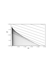
Figure 1: Plot of the lines (2.7) for $\mu$ ranging from $0.4$ (upper right corner) to $75$ (line at the extreme left). The region of overlapping lines corresponds to a region of first order phase transition.

The parameter $\mu$ is now seen to be useful for two different reasons. First it characterizes the general structure of the phase diagram (Fig. 2) where the ‘strong coupling’ regime is the region with $\mu>1$ and the ‘weak coupling’ regime has $\mu<1$. As well, and of more importance for our analysis, we find that the expectation values of traces of powers of the group element $g$ are given as a function of the single parameter $\mu$

$$<{\rm Tr}~{}g^{n}/N>=c_{n}=\frac{I_{n}(\mu)}{I_{0}(\mu)}$$ (2.8)

Consequently, it makes sense for our purposes to re-define the eigenvalue distribution in terms of $\mu$

$$\rho_{0}(\theta,\mu)=\frac{2}{\pi I_{0}(\mu)}\sqrt{\mu+\cos{\theta}}$$ (2.9)

In the next section we will use this definition and its connection to the dominant configuration of the gauge element to analyze the phase diagram in terms of group theory.

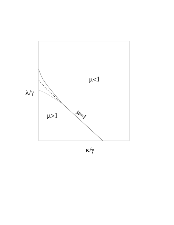
Figure 2: Schematic picture of the phase diagram. The doted curve marks the first order part of the critical line. The solid curves above and below it are the boundaries of the area with two possible phases. They join at a point which shows second order behaviour. For larger $\kappa/\gamma$ we find a third order line ($\mu=1$) marked by a solid line.

3 Order parameters and some group theory

As is known, in the case of pure gluo-dynamics, the realization of the center symmetry of the gauge group governs confinement  [2]. The Polyakov loop operator ${\rm Tr}~{}g(x)$, which is related to the free energy $-T\log{<\rm{Tr}g(x)\rm{Tr}g^{\dagger}(0)>}$ of a conjugate pair of static, external fundamental charges separated by a distance $x$, serves as an order parameter [3] to test confinement. Since ${\rm Tr}~{}g(x)$ transforms under the center as ${\rm Tr}~{}g(x)~{}\rightarrow z~{}{\rm Tr}~{}g(x)$, the expectation value of the Polyakov loop operator must average to zero if the center symmetry is preserved. Physically this suggests that an infinite amount of energy is required to introduce a single fundamental test charge into the system. The presence of a gas of fundamental charges $(\kappa\neq 0)$ changes this situation though by explicitly breaking the center symmetry. Consequently we lose the Polyakov loop operator as an order parameter for phase transitions in the system. In this section we introduce a suitable generalization of the Polyakov loop operator which will allow us to identify a new order parameter.

As seen in the previous section, the solution of the non-Abelian Coulomb gas with adjoint and fundamental representation charges is completely characterized by a Fourier sum of the traces $c_{n}=<{\rm Tr}~{}g^{n}/N>$ - the higher winding Polyakov loops. As noted in [4] the character of these traces changes between the strong and weak coupling regimes. In particular, in the strong coupling $(\mu>1)$ phase $c_{n}$ is damped exponentially with $n$ while in the weak coupling $(\mu<1)$ phase the damping follows a power law behaviour. Now we will reconsider this behaviour in terms of group theory.

Since the matrix $g$ is an element of the special unitary group, its trace in an irreducible representation, $R$ defines the group character for that representation

$$\chi_{R}(g)\equiv{\rm Tr}_{R}~{}g$$ (3.1)

For the $N$ dimensional fundamental representation of $SU(N)$, $F$, the group character is just the Polyakov loop operator described above since we are considering group elements to be taken in the lowest fundamental representation

$$\chi_{F}(g)={\rm Tr}~{}g$$ (3.2)

Further simple examples are the symmetric $(S)$ and anti-symmetric $(A)$ combinations of a pair of fundamentals where we have

$$\chi_{S}(g)=\frac{1}{2}[({\rm Tr}~{}g)^{2}+{\rm Tr}~{}g^{2}]~{}~{},~{}~{}\chi_{A}(g)=\frac{1}{2}[({\rm Tr}~{}g)^{2}-{\rm Tr}~{}g^{2}]$$ (3.3)

A general relation between characters and the group elements is given by the Weyl formula but is not necessary for the following. A complete discussion can be found in standard references (see [18] for example).

The main idea is that the eigenvalues of the group matrices, which are the only relevant dynamical variables in the grand partition function (2.1), are completely determined by the $N$ quantities $\{{\rm Tr}~{}g^{n}\}$, $n=1\ldots N$. In turn these traces form an algebraic basis equivalent to the characters of the $N$ fundamental (completely anti-symmetric) irreducible representations of $SU(N)$ (including the trivial representation). Here we will explicitly demonstrate the relationship between the basis of traces and the basis of group characters. Ultimately it is the group theoretic variables which we will use to characterize the phases of the model (2.1).

The standard basis for general functions (of finite degree) of the eigenvalues of a matrix is the set of elementary symmetric functions $\{a_{r}\}$. In terms of the eigenvalues $\lambda_{j}=~{}{\rm e}^{i\theta_{j}}$ of the group element $g$ they are given by

$$a_{1} = \sum_{j}\lambda_{j}$$ (3.4)

$$a_{2} = \sum_{j<k}\lambda_{j}\lambda_{k}$$

$$a_{3} = \sum_{j<k<l}\lambda_{j}\lambda_{k}\lambda_{l}$$

$$\vdots$$

$$a_{N} = \prod\lambda_{j}=\det{g}=1$$ (3.5)

with $a_{r}\equiv 0$ for $r>N$. The relationship of the symmetric functions $\{a_{r}\}$ to the traces of the group elements, $S_{n}={\rm Tr}~{}g^{n}$, is given [15] by the determinant

$$a_{k}=\frac{1}{k!}\left|\begin{array}[]{ccccccc}S_{1}&1&0&\cdots&&&\\ S_{2}&S_{1}&2&0&\cdots&&\\ S_{3}&S_{2}&S_{1}&3&0&\cdots&\\ \vdots&\vdots&\vdots&\vdots&&&0\\ S_{k-1}&S_{k-2}&S_{k-3}&\cdots&S_{2}&S_{1}&k-1\\ S_{k}&S_{k-1}&S_{k-2}&\cdots&S_{3}&S_{2}&S_{1}\end{array}\right|$$ (3.6)

Most importantly, it can be shown that the elementary symmetric functions are nothing more than the characters of the fundamental representations for the unitary group [15, 16]. That is, for the fundamental representation which is the anti-symmetric combination of $k$, $N$ dimensional representations, $\chi_{k}(g)=a_{k}$.

The determinant (3.6) can be evaluated [17] in terms of a multinomial expansion most compactly stated in terms of a generating function

$$\chi_{k}(g)=\frac{(-1)^{k}}{k!}\frac{d^{k}}{dz^{k}}\left.\exp{[-\sum_{n=1}^{\infty}\frac{{\rm Tr}g^{n}}{n}z^{n}]}\right|_{z=0}$$ (3.7)

For our purposes though it is useful to convert to a contour integral about the origin.

$$\chi_{k}(g)=\frac{(-1)^{k}}{2\pi i}\oint\frac{dz}{z^{k+1}}\exp{\left[-\sum_{n=1}^{\infty}\frac{{\rm Tr}g^{n}}{n}z^{n}\right]}$$ (3.8)

These last two expressions explicitly demonstrate the relationship between the group element $g$ and the $k^{th}$ fundamental representation of the gauge group and are completely general results.

With these relations we see that there is a direct connection between the gauge group element $g$ and the irreducible (fundamental) representations of the gauge group. In particular, in the previous section we have seen that in the large $N$ solution of the non-Abelian Coulomb gas a certain configuration of the gauge matrix, $g_{0}$ saturated the evaluation of the partition function (2.1). Now it is natural to ask what is the configuration of irreducible representations corresponding to the dominant $g_{0}$. This corresponds to evaluating the expectation $<\chi_{k}(g)>$ in the background of the non-Abelian gas. In principle this involves calculating expectations of the form $<{\rm Tr}~{}g^{n_{1}}\cdots{\rm Tr}~{}g^{n_{r}}>$ but because of the factorization of gauge invariant objects in the limit $N\rightarrow\infty$, this reduces to a product of expectations, $<{\rm Tr}~{}g^{n_{1}}>\cdots<{\rm Tr}~{}g^{n_{r}}>$. Consequently $<\chi_{k}(g)>$ is determined by replacing ${\rm Tr}~{}g^{n}$ by its expectation value in (3.8). Of course expectation values of the group element traces are intimately related to the eigenvalue density $\rho(\theta,\mu)$ (see (2.2)) hence, after performing an infinite sum, we obtain

$$<\chi_{\alpha}>[\rho(\theta,\mu)]\equiv\frac{(-1)^{\alpha N}}{2\pi i}\oint\frac{dz}{z}\exp{\left[\frac{N}{2}\int d\theta\rho(\theta,\mu)\log{\left(\frac{1+z^{2}-2z\cos{\theta}}{z^{2\alpha}}\right)}\right]}$$ (3.9)

Note that we have defined a new real parameter $\alpha=k/N$ on the unit interval that effectively labels the fundamental representations in the large $N$ limit. Of course (3.9) now depends on a continuous variable and is of a slightly different functional form than the discrete case $<\chi_{k}>$. In the remainder of this discussion we will consider only the character parameterized by $\alpha$ as defined in (3.9).

4 Calculation of the expectation of fundamentals

In this section we will concentrate on calculating $<\chi_{\alpha}>$ with eigenvalue density (2.9) for the non-Abelian Coulomb gas. This calculation will give a clear picture of the group theoretic excitations present in different regions of the phase diagram and consequently allow us to define an order parameter for the deconfinement transition even in the presence of fundamental matter.

Since explicit evaluation of (3.9) is difficult we begin with some special limiting cases. As $\mu\rightarrow-1$ the support of the eigenvalue distribution (2.9) vanishes at $\theta=0$. The distribution does not vanish though as it retains unit normalization and effectively becomes a delta function, $\delta(\theta)$. Consequently we find the gauge matrix $g$ is just the identity at $\mu=-1$, hence

$$<\chi_{\alpha}>=\lim_{N\rightarrow\infty}\left(\begin{array}[]{c}N\\ \alpha N\end{array}\right)=2^{N}\sqrt{\frac{2}{N\pi}}~{}{\rm e}^{-2N(\alpha-1/2)^{2}}$$ (4.1)

In this limit we find that the distribution of characters is symmetric about $\alpha=1/2$ as one would expect in a system where the total colour charge is vanishing. As well in this limit $<\chi_{\alpha}>$ is non-vanishing and all fundamental representations are present in the large $N$ background solution of the model. As we will see, this result is generic in the weak coupling phase $\mu<1$.

In the opposite limit, as $\mu\rightarrow\infty$, it can be shown that the eigenvalue distribution (2.9) approaches a constant value $\rho=1/2\pi$ with the eigenvalues of the group element $g$ becoming uniformly distributed on the unit circle. Since expectation values of the traces of powers of the gauge matrix are essentially Fourier transforms of the eigenvalue distribution, it is easy to see that $<{\rm Tr}~{}g^{n}>\rightarrow 0$ in this limit and

$$<\chi_{\alpha}>\rightarrow\delta_{0,\alpha}$$ (4.2)

This limit corresponds to the extreme strong coupling phase of the model where the Polyakov loop operator $(<{\rm Tr}~{}g>\sim<\chi_{1/N}>)$ has vanishing expectation value and the standard analysis would point to a phase where colour charges are strictly confined into hadron-like structures.

In general the integral (3.9) can be evaluated by saddle-point methods in the large $N$ limit in which we are interested. The relevant action in this limit is

$$S(\alpha,\mu,z)=\int d\theta\rho(\theta,\mu)\log{\left(\frac{1+z^{2}-2z\cos{\theta}}{z^{2\alpha}}\right)}$$ (4.3)

Solving the stationarity condition, $dS/dz|_{z_{0}}=0$, for $\alpha$ in terms of $z_{0}$ we find the saddle-point condition for the large $N$ behaviour of the integral (3.9) is given by the relationship

$$\alpha=\int d\theta\rho(\theta,\mu)\frac{z_{0}(z_{0}-\cos{\theta})}{1+z_{0}^{2}-2z_{0}\cos{\theta}}$$ (4.4)

Since $\alpha$ is a real parameter restricted to the unit interval $[0,1]$ it can be shown that the saddle-point value of the parameter $z_{0}$ is real. Further, for $z_{0}>1$ and $0<z_{0}<1$ Eqn.4.4 returns values of $\alpha>1$ and $\alpha<0$, respectively. Consequently we need only consider real, negative values of the parameter $z_{0}$.

We now turn to an examination of the saddle-point approximation of (3.9) for different regions of the phase diagram of the model at hand beginning with the weak coupling phase, $\mu<1$. In this case the support of the eigenvalue distribution (2.9) is bounded away from $\theta=\pm\pi$ and hence the denominator in (4.4) is non-singular for all values of $z_{0}$. Consequently, in this regime $\alpha$ varies smoothly and monotonically with $z_{0}$ and the relation (4.4) can in principle be inverted to obtain $z_{0}(\alpha)$. With this information, the large $N$ asymptotic form of the expectation value of the characters $<\chi_{\alpha}>$ can be determined by standard saddle-point methods. In Figure 3 we show a numerically calculated example of $\alpha$ as a function of $z_{0}$ for $\mu=0.5$. For this same case we show a schematic diagram of the magnitude of the expectation value $|<\chi_{\alpha}>|$ as a function of $\alpha$ in Figure 4. In particular we see that the system has excitations in all irreducible representations.

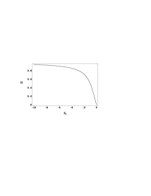
Figure 3: Saddle-point relation for $\mu=0.5$

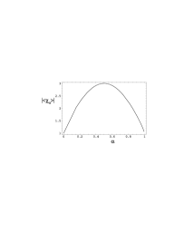
Figure 4: Schematic diagram of $|<\chi_{\alpha}>|$ vs. $\alpha$ for $\mu=0.5$

For $\mu>1$ the situation is somewhat different. Now the support of the eigenvalue distribution (2.9) is the full interval $\theta\in[-\pi,\pi]$, and the denominator of (4.4) causes non-analytic behaviour to appear. As one increases $\mu$ through unity the saddle-point relation for $\alpha$ shows this non-analytic behaviour as a discontinuity at $z_{0}=-1$ (see Figure 5). The result is that an open interval of $\alpha$ values centered on $\alpha=1/2$ are mapped into this discontinuity when the saddle-point relation (4.4) is inverted. Since this discontinuity occurs in the saddle-point relation, it is not surprising to find that the curvature associated with the Gaussian integration of the saddle-point approximation is divergent, effectively forcing the integral to vanish. In terms of the expectation values of different representations in the background of the non-Abelian Coulomb gas, we see that an open interval of fundamental representations centered about $\alpha=1/2$ is missing from the spectrum in the large $N$ limit. In Figure 6 we show an example of the behaviour of the expectation value $|<\chi_{\alpha}>|$ with $\alpha$ for $\mu=1.2$.

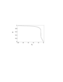
Figure 5: Saddle-point relation for $\mu=1.2$

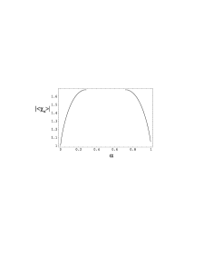
Figure 6: Schematic diagram of $|<\chi_{\alpha}>|$ vs. $\alpha$ for $\mu=1.2$

The main outcome of this analysis is that the expectation value of the central fundamental character $<\chi_{1/2}>$ is vanishing if and only if $\mu\geq 1$. Consequently it may be considered an order parameter distinguishing between the strong and weak coupling phases of the model. Physically the situation is clear. In the weak coupling phase the system can effectively screen the interactions of any pair of charges regardless of their representation since the system contains excitations in all representations of the gauge group. We conclude that the system looks much like a quark-gluon plasma where charges are effectively deconfined. At the phase transition line non-Abelian flux in the $\alpha=1/2$ fundamental representation becomes too energetically costly to produce and the system can no longer screen the interaction between a pair of $\alpha=1/2$ fundamental charges. In this strong coupling phase the interacting pair sees a linear confining potential (though somewhat reduced as compared to the empty background). As one further increases $\mu$ the gap in the spectrum of fundamental representations becomes larger and in the extreme limit $\mu=\infty$ the system contains only excitations in the trivial representation. This is precisely the confining phase of pure gluo-dynamics.

5 Discussion

As we have shown, the generalization of the concept of the Polyakov loop operator to probe the group theoretic excitations of a system of non-Abelian electric charges provides a convenient and unified way to quantify the physics of phase transitions. While the details of our presentation have centered on a two dimensional model with an infinite number of colours, the general concepts developed here should be applicable to interacting gauge systems in arbitrary dimensions for both infinite and finite rank $(N)$ gauge groups. Unfortunately we are unable to test these ideas in a solvable two dimensional model as for finite $N$ there is no phase transition and the system is always in the deconfined phase where all representations are present.

One immediate problem with using the fundamental representations to characterize the phase diagram arises when considering finite, odd rank groups. For example in the physically relevant case of $SU(3)$, there are only two fundamental representations $k=1,2$ and the order parameter $<\chi_{1/2}>$ would naively denote the $k=3/2$ fundamental representation. In terms of group theory this fractional representation is nonsense and strongly suggests that direct application of the large $N$ results is not prudent. Even worse is the fact that a finite number of representations are not enough degrees of freedom to describe the change in character of the group elements from $g\sim 1$ in the weak coupling phase to $g$ away from the identity in the strong coupling phase. Alternatively, we are free to use any independent set of irreducible representations to characterize the system. In particular the completely symmetric representations provide an equivalent algebraic basis to the fundamentals we have considered here. The strength of this approach is that there is no restriction on the number of symmetric representations for the unitary groups contrasting the $N-1$ fundamental representations for $SU(N)$. Unfortunately, repeating the calculations of Section 4 with symmetric representations one discovers that there is no strong signal for the phase transition and in particular one cannot define an order parameter.

Despite the apparent difficulties with applying the current results to finite rank gauge theories, we feel that the general concept of characterizing the phases of a gauge theory coupled to matter by the spectrum of higher irreducible representations is useful. In particular it would be interesting to investigate these ideas in the setting of lattice calculations of gauge theories that are known to possess phase transitions. In fact, for the case of $SU(2)$ gauge theory, the $J=1/2,1$ and $3/2$ Polyakov loops have been calculated on the lattice [19] (see also [20]). It would certainly be very instructive to have more complete information about the higher representation Polyakov loops in this simple model both with and without fundamental representation matter.

References

-
[1]
N. Weiss, Phys. Rev. D35 (1987), 2495;
A. Roberge and N. Weiss, Nucl. Phys. B275 (1986), 734;
D.E. Miller and K Redlich, Phys Rev. D37 (1988), 3716. -
[2]
A. M. Polyakov, Phys. Lett. B72 (1978), 477;
L. Susskind, Phys. Rev. D20 (1979), 2610. -
[3]
B. Svetitsky and L. Yaffe, Nucl. Phys.
B210 (1982), 423;
B. Svetitsky, Phys. Rept. 132 (1986), 1. - [4] C. Gattringer, L. Paniak and G. Semenoff, Ann. Phys. 256 (1997), 74; hep-th/9612030.
- [5] D. Gross and E. Witten, Phys. Rev. D21 (1980), 446.
- [6] M. Douglas and V. Kazakov, Phys. Lett. B319 (1993), 219; hep-th/9305047.
- [7] D. Gross and A. Matytsin, Nucl. Phys. B437 (1995), 541; hep-th/9410054.
-
[8]
A. Lenard, J. Math. Phys. 2 (1961), 682;
Y. Nambu, B. Bambah and M. Gross, Phys. Rev. D26 (1982), 2875;
M. Engelhardt, hep-th/9701105. - [9] T. Banks and A. Ukawa, Nucl. Phys. B225 (1983), 145.
- [10] K. Zarembo, Mod. Phys. Lett. A10 (1995), 677; hep-th/9405080.
-
[11]
G. W. Semenoff, O. Tirkkonen and K. Zarembo,
Phys. Rev. Lett. 77 (1996), 2174; hep-th/9605172;
G. W. Semenoff and K. Zarembo, Nucl. Phys B480 (1996), 317; hep-th/9606117;
G. Grignani, G. W. Semenoff and P. Sodano, Phys. Rev. D53 (1996), 7157; hep-th/9504105. - [12] E. Brezin, C. Itzykson, G. Parisi and J.-B. Zuber, Commun. Math. Phys. 59 (1979), 35.
-
[13]
A. Jevicki and B. Sakita, Phys. Rev. D22
(1980) 467;
S.R. Wadia, Phys. Lett. 93B (1980) 403;
S.R. Das and A. Jevicki, Mod. Phys. Lett. A5 (1990), 1639. - [14] S. Gubser and I. Klebanov, Phys. Lett. B340 (1994), 35; hep-th/9407014.
- [15] D. E. Littlewood, The Theory of Group Characters, second edition. University of Oxford Press, Oxford, 1958.
- [16] C. R. Hagen and A. J. Macfarlane, J. Math. Phys. 6 (1965), 1355.
- [17] T. Muir and W. Metzler, Theory of Determinants , Albany NY, 1930.
- [18] H. Weyl, The Classical Groups, Princeton Univ. Press, Princeton, N.J. , 1946.
- [19] J. Kiskis, Phys. Rev. D41 (1990), 3204.
- [20] P.H. Damgaard and M. Hasenbusch, Phys. Lett. B331 (1994), 400; hep-lat/9404008.