CERN-TH/97-144

US-FT-21/97, UB-ECM-PF 97/10

hep-th/9707017

June 1997

SOFTLY BROKEN $N=2$ QCD

WITH MASSIVE QUARK HYPERMULTIPLETS, II

Luis Álvarez-Gaumé^a, Marcos Mariño^b and Frederic Zamora^a,c.

^a Theory Division, CERN,
1211 Geneva 23, Switzerland.

^b Departamento de Física de Partículas,
Universidade de Santiago de Compostela,
E-15706 Santiago de Compostela, Spain.

^c Departament d’Estructura i Constituents de la Materia,
Facultat de Física, Universitat de Barcelona,
Diagonal 647, E-08028 Barcelona, Spain.

Abstract

We analyze the vacuum structure of $N=2$, $SU(2)$ QCD with massive quark hypermultiplets, once supersymmetry is soflty broken down to $N=0$ with dilaton and mass spurions. We give general expressions for the low energy couplings of the effective potential in terms of elliptic functions to have a complete numerical control of the model. We study in detail the possible phases of the theories with $N_{f}=1,2$ flavors for different values of the bare quark masses and the supersymmetry breaking parameters and we find a rich structure of first order phase transitions. The chiral symmetry breaking pattern of the $N_{f}=2$ theory is considered, and we obtain the pion Lagrangian for this model up to two derivatives. Exact expressions are given for the pion mass and $F_{\pi}$ in terms of the magnetic monopole description of chiral symmetry breaking.

1 Introduction

This is the second part of a series of papers where we study the soft breaking of $N=2$ QCD with massive matter. In the first paper of the series [1] (referred as (I) from now on) we focused on two well differentiated but necessary goals. The first one was to have complete numerical control of the exact Seiberg-Witten solution for $SU(2)$ gauge group and $N_{f}\leq 3$ massive quark hypermultiplets. We presented a general framework to obtain explicit expresions for the Seiberg-Witten periods $(a_{D}(u),a(u))$ and all the effective couplings of the nonsupersymmetric low energy effective Lagrangian at any point of the $u$-plane. This powerful method was based on the use of uniformization theory for the Seiberg-Witten elliptic curves.

The second goal of the first paper was to study the logic of the general soft breaking of massive $N=2$ QCD down to $N=0$ by the introduction of $N=2$ spurion fields. We promoted the masses in the bare Lagrangian to $N=2$ vector superfields by gauging the baryon numbers of the quark hypermultiplets. We obtained an effective $SU(2)\times U(1)^{N_{f}}$ Seiberg-Witten model, where the dynamics of the $N_{f}$ $U(1)$ baryon gauge symmetries is frozen and we turn on the auxiliary fields of the corresponding $N=2$ vector superfields to get additional supersymmetry breaking parameters. We also embedded the effective $SU(2)\times U(1)^{N_{f}}$ Seiberg-Witten model into a pure gauge theory with higher rank group, where the additional degrees of freedom with “magnetic” baryon numbers different from zero, became infinitely heavy and decoupled in a limiting region of the moduli space. We analysed in full detail all the monodromy properties and the internal consistency of these softly broken models. Finally, we gave the general expression of the exact effective potential of the softly broken theory when both dilaton and mass spurions are included.

In this second paper, we perform a complete analysis of the nonperturbative vacuum structure and the large distance physics of the softly broken $N=2$ massive QCD. The structure of the paper is the following:

In section 2 we present the $N=2$ soft breaking terms of the bare Lagrangian and discuss their main physical features. For completeness, we also give the final formulae for $(a_{D}(u),a(u))$, the dual mass $m_{D}$, and all the effective couplings, $\tau^{AB}$, in terms of elementary elliptic functions. These explicit formulae can be implemented numerically in the Mathematica program. This makes possible the extraction of the nonperturbative effects encoded in the nonsupersymmetric effective potential and to unveil the rich phase structure of these models. At the end of the section, we give an exact expresion of the squark condensates $<{\tilde{q}}_{f}q_{f}>$, the “electric” order parameters of chiral symmetry breaking, in terms of the low energy couplings and the monopole condensate.

In section 3, we focus on the vacuum structure with one massive quark hypermultiplet. The phase structure of the theory depends on the values of the bare mass $m$, and the two supersymmetry breaking parameters: $f_{0}$ for the dilaton spurion and $f_{m}$ for the mass spurion. The phase diagram is divided in two well defined regions. When $m<m_{c}$, where $m_{c}$ is the critical mass for the Argyres-Douglas point to occur [9], the theory is in different Higgs-confining phases. There are first order phase transitions among these phases associated to the condensation of “bound states” made of mutually non-local degrees of freedom, with total magnetic charge $n_{m}=2$ or $n_{m}=3$. For $m>m_{c}$, when only the dilaton spurion is turned on,

the vacuum structure flows to the pure $SU(2)$ one analysed in [4] an expected result because of the quark decoupling under the flow of the renormalization group. The theory is then in a “magnetic”, confining phase. But when supersymmetry is broken with the mass spurion $f_{m}$, the ground state is associated to an elementary quark condensate. This purely “electric” vacuum goes to infinity in the $u$-plane as the mass is increased, and in the decoupling limit we obtain a flat potential. The moduli space of vacua of $N=2$ supersymmetric Yang-Mills theory [2] is then recovered.

In the rest of the paper we focus on the nonperturbative physics at large distance of the $N_{f}=2$ theory with small bare masses. In this case we have a QCD-like situation, where the number of light flavors is equal to the number of colors. For massless quark hypermultiplets, the flavor symmetry group is $SU(2)_{-}\times SU(2)_{+}$. At low energy, the relevant degrees of freedom are light magnetic BPS states in flavor group representations $({\bf 2},{\bf 1})$ or $({\bf 1},{\bf 2})$. Chiral symmetry breaking is then driven by the condensation of these light monopoles [3].

In section 4 we present the phase structure of the $N_{f}=2$ softly broken theory, as a function of the different values of the dilaton and mass spurions. For supersymmetry breaking dominated by the dilaton spurion, the vacuum is in the magnetic region $u\sim\Lambda^{2}_{2}/8$, with first order phase transitions between mutually local minima as the values of the mass spurions are slightly changed. The pattern of chiral symmetry breaking is $SU(2)_{-}\times SU(2)_{+}\rightarrow SU(2)_{+}$. If the supersymmetry breaking is dominated by the mass spurions, there is a new kind of first order phase transition between mutually non-local minima. The minimum can jump from the monopole to the dyon region $u\sim-\Lambda^{2}_{2}/8$, and in this way the opposite pattern of chiral symmetry breaking $SU(2)_{-}\times SU(2)_{+}\rightarrow SU(2)_{-}$ is realized. Finally, we show that there are critical values of the bare masses such that a new minima is generated at $u=0$, due to the condensation of a “bound state” in the $({\bf 2},{\bf 1})\bigoplus({\bf 1},{\bf 2})$ representation of the flavor group. This could be an indication of a new phase where the pattern of chiral symmetry breaking is $SU(2)_{-}\times SU(2)_{+}\rightarrow SU(2)_{V}$.

Finally, in section 5 we give the pion Lagrangian up to two derivatives, for the chiral symmetry breaking pattern $SU(2)_{-}\times SU(2)_{+}\rightarrow SU(2)_{+}$. We obtain expresions for the pion decay constant $F_{\pi}$ and the pion masses $M_{\pi}$ in terms of the bare quark masses and the supersymmetry breaking parameters. This gives a connection between these phenomenological parameters and the magnetic monopole description of chiral symmetry breaking. We think that, although the model we study has many obvious differences with respect to ordinary QCD, some features of this connection can be present in more realistic models. The pion Lagrangian parameters we obtain are intrinsically nonperturbative, and they have a natural expansion in terms of inverse powers of the dynamically generated scale $\Lambda$.

2 Soft breaking of $N=2$ QCD with Massive Quark Hypermultiplets

2.1 Breaking supersymmetry. The Bare Lagrangian

To break $N=2$ supersymmetry down to $N=0$ in the $SU(2)$ theory with $N_{f}$ flavors , we promote the scale $\Lambda_{N_{f}}$ [4, 5] and the masses $m_{f}$ [1] to $N=2$ vector superfields, and then we freeze the scalar and auxiliary components to be constants. The dilaton spurion is introduced through the relation $\Lambda_{N_{f}}=\mu_{0}{\rm e}^{iS}$, with $\mu_{0}$ the UV cut-off scale of the bare Lagrangian. The RG equation for the $SU(2)$ theory with $N_{f}$ hypermutliplets gives the relation $\Lambda_{N_{f}}^{4-N_{f}}\sim{\rm e}^{i\tau}$, where we use the normalization of [3] for the coupling constant, $\tau=8\pi i/g^{2}+\theta/\pi$. We then obtain $s=\pi\tau/(4-N_{f})$, and the spurion superfield $S$ appears in the classical prepotential as

$${\cal F}={4-N_{f}\over 2\pi}SA^{2}.$$ (2.1)

The bare Lagrangian reads, once the auxiliary fields of the dynamical superfields are integrated out,

$${\cal L}={\cal L}_{N=2}+(4-N_{f})\Bigg{[}{\rm Im}\Big{(}{F_{0}\over 8\pi^{2}}\lambda\lambda+{{\overline{F}}_{0}\over 8\pi^{2}}\psi\psi\Big{)}+{{\sqrt{2}}D_{0}\over 8\pi^{2}}{\rm Im}\Big{(}i\lambda\psi\Big{)}\Bigg{]}$$

$$-{(4-N_{f})D_{0}\over\pi{\rm Im\tau}}f_{abc}({\rm Im}\phi^{a})\phi^{b}{\bar{\phi}}^{c}-{(4-N_{f})\over\pi{\rm Im}\tau}\Big{(}F_{0}{\tilde{q}}_{f}({\rm Im}\phi)q_{f}+{\rm h.c.}\Big{)}$$

$$-{(4-N_{f})D_{0}\over\pi{\rm Im\tau}}\Big{(}{q}^{\dagger}_{f}({\rm Im}\phi)q_{f}-{\tilde{q}}_{f}({\rm Im}\phi){\tilde{q}}^{\dagger}_{f}\Big{)}$$

$$-{(4-N_{f})^{2}\over 4\pi^{3}{\rm Im\tau}}\Big{(}{1\over 2}D_{0}^{2}+|F_{0}|^{2}\Big{)}({\rm Im}\phi)^{2}$$

$$+{\sqrt{2}}S_{f}\Big{(}F_{f}{\tilde{q}}_{f}q_{f}+{\rm h.c.}\Big{)}+S_{f}D_{f}(|q_{f}|^{2}-|{\tilde{q}}_{f}|^{2}).$$ (2.2)

In this Lagrangian, $\lambda$, $\psi$ are the gluinos, $\phi$ is the scalar component of the $N=2$ vector superfield, and $q_{f}$, ${\tilde{q}}_{f}$ are the squarks. The constants $S_{f}$ are the baryon numbers of the quark hypermultiplets. In the numerical study of the model, we set them equal to one. As the prepotential has an analytic dependence on the spurion superfields, the effective Lagrangian up to two derivatives and four fermions terms for the $N=0$ theory described by (2.2) is given by the exact Seiberg-Witten solution once the spurion superfields are taken into account. This gives the exact effective potential at leading order and the vacuum structure can be determined.

Notice that the terms involving mass spurions can be regarded as additional mass terms for the squarks, but not all of them are positive definite. More precisely, the graded trace of the mass matrix still vanishes after this soft breaking of supersymmetry, and the additional mass terms for the squarks are grouped in pairs with opposite signs. This is apparent in the $D_{f}$ terms in (2.2). We then expect a vacuum structure similar to the one found in [7] for the soft breaking of $N=1$ supersymmetry, although here the structure is more complicated due to the presence of the Higgs field $\phi$. These kinds of terms have two consequences for the vacuum structure of the theory: first, for certain values of the spurions and the masses the resulting potential can be unstable, as the vacuum energy can be unbounded from below. Second, these terms favour an squark condensate in a Higgs phase. Both issues were discused in [7] in the context of $N=1$ supersymmetry, and here we will adress them using the exact effective potential of the theory.

In general, the bare Lagrangian (2.2) will not be CP invariant, since $\tau,m_{f},F^{A}$ are arbitrary complex parameters. There are some particular situations where we still can have CP invariance. We can asign to the bare masses $m_{f}$ and the spurion dilaton $F_{0}$ an $R$-charge two. If these parameters have the same complex phase, we can perform an anomalous $U(1)_{R}$ transformation such that for a value of the bare $\theta$ angle, CP is a symmetry of the bare Lagrangian. The other situation where CP is not lost is when $\theta$ is equal zero, the bare quark masses $m_{f}$ are real and positive and all supersymmetry breaking parameters $F^{A}$, $A=0,1,...,N_{f}$, have the same complex phase. In this case, we can make a non anomalous transformation on the phases of the squarks and the gluinos such that the common complex phase of all the spurions $F^{A}$ is set to zero. These are the two main situations where we still keep CP symmetry, where genericaly, because of $u=<{\rm Tr}\phi^{2}>\not=0$, the vacuum will break CP spontaneously. We will find such vacua in sections 2 and 3. But for complex bare masses and supersymmetry breaking parameters with relative complex phases among them, we do not have CP invariance in the bare Lagrangian. In those cases, we will get effective Lagrangians at low energy which are not CP invariant.

2.2 The Low Energy Effective Couplings

In (I), a general procedure to compute the Seiberg-Witten periods was introduced, based on the uniformization of the elliptic curve associated to the theory . In this way we have a map from the ${\bf C}/\Lambda$ lattice to the $(x,y)$ variables of the Seiberg-Witten curve through the $\wp(z)$ Weierstrass elliptic function. The variables are given by

$$x=4\wp(z)+{u\over 3}+{\delta_{N_{f},3}\over 192}\Lambda_{3}^{2},\,\,\,\,\,\,\,\ y=4\wp^{\prime}(z).$$ (2.3)

The Seiberg-Witten abelian differential can be written as

$$\lambda_{SW}={{\sqrt{2}}\over 8\pi}{dx\over y}(2u-(4-N_{f})x)+{dx\over y}\sum_{n=1}^{N_{p}}{r_{n}\over x-x_{n}}.$$ (2.4)

In this equation, $N_{p}$ denotes the number of poles (which depends on $N_{f}$), located at $x_{n}$, and the coefficients $r_{n}$ are given by

$$r_{n}=4\wp^{\prime}(z_{n})[{\rm Res}_{x=x_{n}}\lambda_{SW}],$$ (2.5)

where the $z_{n}$ correspond to the poles $x_{n}$ through (2.3). The residues can be written as linear combinations of the masses, and this defines the coefficients $S_{n}^{f}$ as follows:

$${\rm Res}_{x=x_{n}}\lambda_{SW}={1\over 2\pi i}\sum_{f=1}^{N_{f}}S_{n}^{f}{m_{f}\over{\sqrt{2}}}.$$ (2.6)

The explicit values of $\wp^{\prime}(z_{n})$ and $S_{n}^{f}$ can be found in (I).

Denoting $a_{1}=a_{D}$, $a_{2}=a$, one can integrate (2.4) over the basic homology cycles to obtain the explicit expressions

$$a_{i} = {{\sqrt{2}}\over\pi}\Big{(}(4-N_{f})\zeta({\omega_{i}\over 2})+({N_{f}+2\over 24})u\,\omega_{i}-({\delta_{N_{f},3}\Lambda_{3}^{2}\over 1536})\omega_{i}\Big{)}$$ (2.7)

$$+ 2i\sum_{n=1}^{N_{p}}[{\rm Res}_{x=x_{n}}\lambda_{SW}]\big{[}\omega_{i}\zeta(z_{n})-2z_{n}\zeta\big{(}{\omega_{i}\over 2}\big{)}\big{]},$$

where $\zeta(z)$ is the Weierstrass zeta-function, and $\omega_{i}$ are the periods of the abelian differential $dx/y$. Expressions for the derivatives of $\lambda_{SW}$ w.r.t. the masses can be easily found, and these give in turn

$$\Big{(}{\partial a_{i}\over\partial m_{f}}\Big{)}_{u}={1\over{\sqrt{2}}}\sum_{n=1}^{N_{p}}{S_{n}^{f}\over\pi i}\big{[}\omega_{i}\zeta(z_{n})-2z_{n}\zeta\big{(}{\omega_{i}\over 2}\big{)}\big{]}.$$ (2.8)

Using the Riemann bilinear relations, one can obtain an equation for the dual mass (I),

$$m_{D}^{f}={\sqrt{2}}\Big{(}{\partial{\cal F}(a,m_{f})\over\partial m_{f}}\Big{)}_{a}=\sum_{n=1}^{N_{p}}S^{f}_{n}\int_{x^{-}_{n}}^{x^{+}_{n}}\lambda_{SW},$$ (2.9)

where ${\cal F}(a,m_{f})$ is the Seiberg-Witten prepotential for the massive theories, and the points $x^{+}_{n}$ and $x^{-}_{n}$ ($n=1,\cdots,N_{p}$) are the simple poles of $\lambda_{SW}$ at each of the two Riemann sheets. The ${\sqrt{2}}$ factor arises because it is more convenient to use $m_{f}/{\sqrt{2}}$ as mass variables, given our normalizations. The expression (2.9) is defined up to an $a$-independent constant, that we will set to zero. As it has been remarked in [16], this expression has to be regularized in order to get a finite result, but in our approach via elliptic funtions this can be easily implemented (see (I, 3.30)). We make the simple choice $z_{n}^{-}=-z_{n}^{+}$, and denote $z_{n}^{+}=z_{n}$. We then obtain:

$$m_{D}^{f} = \sum_{n=1}^{N_{p}}S_{n}^{f}\Bigg{(}{{\sqrt{2}}\over\pi}\Big{(}(4-N_{f})\zeta(z_{n})+({N_{f}+2\over 12})u\,z_{n}-({\delta_{N_{f},3}\Lambda_{3}^{2}\over 768})z_{n}\Big{)}$$ (2.10)

$$+ [{\rm Res}_{x=x_{n}}\lambda_{SW}]\big{[}4z_{n}\zeta(z_{n})-2{\rm log}\sigma(2z_{n})\big{]}\Bigg{)}$$

$$+ \sum_{n\not=m}^{N_{p}}S_{n}^{f}[{\rm Res}_{x=x_{m}}\lambda_{SW}]\big{[}4z_{n}\zeta(z_{m})-2{\rm log}{\sigma(z_{n}-z_{m})\over\sigma(z_{n}+z_{m})}\big{]},$$

where $\sigma(z)$ is the Weierstrass sigma-function.

Using these expressions it is easy to check that

$$a_{D}{\partial a\over\partial u}-a{\partial a_{D}\over\partial u}-\sum_{f=1}^{N_{f}}{m_{f}\over{\sqrt{2}}}{\partial m_{D}^{f}\over\partial u}=-i{4-N_{f}\over 4\pi},$$ (2.11)

which is essentially the relation derived in [1, 15, 16].

Once supersymmetry is softly broken with dilaton and mass spurions as in (I), the low-energy effective potential is described in terms of a series of couplings. These can also be written in terms of elliptic functions using (I, 3.36-3.40). We will choose the “electric” description, although the magnetic one can be obtained either by direct computation or by using the generalized duality transformations in (I, 3.14):

$$\tau^{aa} = \frac{\partial^{2}{\cal F}}{\partial a^{2}}={{\omega_{1}}\over{\omega_{2}}},$$

$$\tau^{af} = \frac{\partial^{2}{\cal F}}{\partial a\partial m_{f}}={2\over\omega_{2}}\sum_{n=1}^{N_{p}}S_{n}^{f}z_{n},$$

$$\tau^{0a} = \frac{\partial^{2}{\cal F}}{\partial a\partial s}={{\sqrt{2}}\over\omega_{2}}(4-N_{f}),$$

$$\tau^{0f} = \frac{\partial^{2}{\cal F}}{\partial m_{f}\partial s}=-{\sqrt{2}}(4-N_{f})\sum_{n=1}^{N_{p}}{S_{n}^{f}\over\pi i}\big{[}\zeta(z_{n})-{2z_{n}\over\omega_{2}}\zeta\big{(}{\omega_{2}\over 2}\big{)}\big{]},$$

$$\tau^{00} = \frac{\partial^{2}{\cal F}}{\partial s^{2}}=i{(4-N_{f})^{2}\over\pi}\Big{(}{u\over 12}-{2\over\omega_{2}}\zeta\big{(}{\omega_{2}\over 2}\big{)}\Big{)}+i\delta_{N_{f},3}{\Lambda_{3}^{2}\over 256\pi},$$

$$\tau^{fg} = \frac{\partial^{2}{\cal F}}{\partial m_{f}\partial m_{g}}=-\sum_{n=1}^{N_{p}}{S_{n}^{f}S_{n}^{g}\over\pi i}\big{[}{\rm log}\sigma(2z_{n})-{4z_{n}^{2}\over\omega_{2}}\zeta\big{(}{\omega_{2}\over 2}\big{)}\big{]}$$ (2.12)

$$+ \sum_{n\not=m}^{N_{p}}{S_{n}^{f}S_{n}^{g}\over\pi i}\big{[}{\rm log}{\sigma(z_{n}-z_{m})\over\sigma(z_{n}+z_{m})}+{4z_{n}z_{m}\over\omega_{2}}\zeta\big{(}{\omega_{2}\over 2}\big{)}\big{]}.$$

In $\tau^{fg}$, the divergences have been subtracted following the method explained in (I). Notice that the $z_{n}$ variables are defined up to a shift of an integer linear combination of the periods ${\omega}_{i}$, $i=1,2$, and the $SL(2,{\bf Z})$ group acts in a natural way on the ${\omega}_{i}$, $i=1,2$. One can easily check from the above expressions for the $a_{i}$ that these two sets of transformations (shifts in $z_{n}$ and $SL(2,{\bf Z})$ transformations) combine together to give the inhomogeneous duality transformations of the Seiberg-Witten model for the massive theories [3]. In fact, the generalized duality transformations (I, 3.14) for the couplings can be derived in terms of these geometrical transformations by using the explicit expressions in (2.12).

2.3 The Squark Condensates

The squark condensates can be exactly computed in terms of these couplings, starting from the expression for the bare Lagrangian (2.2) and regarding the supersymmetry breaking parameters $F^{f}$ as source terms. We have:

$$\langle{\tilde{q}}_{f}q_{f}\rangle=-{1\over{\sqrt{2}}}{\partial V_{{\rm eff}}\over\partial F_{f}}={1\over{\sqrt{2}}}\Bigl{(}b_{fB}-{b_{af}b_{aB}\over b_{aa}}\Bigr{)}{\overline{F}}_{B}+\Big{(}S_{i}^{f}-{b_{af}\over b_{aa}}\Big{)}<h_{i}{\tilde{h}}_{i}>,$$ (2.13)

where we follow the notation in (I). Namely, $b_{\alpha\beta}={\rm Im}\tau_{\alpha\beta}/4\pi$, where $\alpha$, $\beta=a,0,f$, $A$,$B=0,f$, and $h_{i}$, ${\tilde{h}}_{i}$ are the scalar components of the $i=1,\cdots,k$ hypermultiplets becoming massless near a singularity, with baryon numbers $S_{i}^{f}$. Using this expression we can compute the squark condensate at the minimum of the effective potential, and in this way we have an additional indication of the “Higgsing” effect of the soft breaking terms.

3 $N_{f}=1$ Vacuum Structure

In this section we study the phase diagram and vacuum structure of the softly broken $N=2$ QCD with one massive hypermultiplet. The massless case was studied in [5], for the soft breaking induced solely by the dilaton spurion. It was found that the theory has generically two degenerate minima with dyon condensation, and at a certain value of the supersymmetry breaking parameter there is a first order phase transition to a single minimum. This new vacuum shows simultaneous condensation of mutually non-local states and has a natural interpretation in terms of oblique confinement [17]. In fact, the two dyons condensing there have opposite electric charges and magnetic number $n_{m}=1$. We will see more examples of these “bound states” in the massive models.

We will study in some detail the theories with arbitrary hypermultiplet mass $m$ and one of the two spurion fields turned on. Two different cases will be considered, with parameter space given by $(m,f_{0})$ and $(m,f_{m})$, respectively. For simplicity, the supersymmetry breaking parameters and the mass will be real and positive, although the most interesting physical phenomena are already captured in these simple cases. In the first subsection we will give the explicit expressions for the monopole condensate and the effective potential. In the second subsection we will analyze the theory with the dilaton spurion breaking parameter $f_{0}$. In the third subsection we will focus on the special case $m=0$ and with only the mass spurion breaking the supersymmetry down to $N=0$. Finally, in the last subsection we will study the phase structure of the theory for general $m$ and $f_{m}$.

3.1 Condensates and effective potential

The general expression for the effective potential of the softly broken theory has been given in (I, 4.7). For $N_{f}=1$ there is only one massless BPS state near each singularity [3], and one has:

$$V_{{\rm eff}} = \Bigl{(}{b_{aA}b_{aB}\over b_{aa}}-b_{AB}\Bigr{)}\Bigl{(}{1\over 2}D_{A}D_{B}+F_{A}{\overline{F}}_{B}\Bigr{)}+{b_{aA}\over b_{aa}}D_{A}(|h|^{2}-|{\widetilde{h}}|^{2})$$ (3.1)

$$+ {\sqrt{2}b_{aA}\over b_{aa}}\Bigl{(}F_{A}h{\widetilde{h}}+{\overline{F}}_{A}{\overline{h}}{\overline{\widetilde{h}}}\Bigr{)}+{1\over 2b_{aa}}(|h|^{2}+|{\widetilde{h}}|^{2})^{2}$$

$$- D_{m}S(|h|^{2}-|{\widetilde{h}}|^{2})+2|a+S{m\over{\sqrt{2}}}|^{2}(|h|^{2}+|{\widetilde{h}}|^{2})$$

$$- \sqrt{2}\Bigl{(}SF_{m}h{\widetilde{h}}+S{\overline{F}}_{m}{\overline{h}}{\overline{\widetilde{h}}}\Bigr{)}.$$

The $A,B=0,m$ labels refer to the mass and dilaton spurions. We will set $D_{0}=D_{m}=0$ for simplicity. Anyway, because of the $SU(2)_{R}$ covariance of (3.1), the monopole solution which minimizes the potential for a general spurion configuration is just the adequate $SU(2)_{R}$ rotation of the solution we will obtain here.

Minimizing w.r.t the monopole fields one obtains the equations

$${\partial V_{{\rm eff}}\over\partial{\overline{h}}}={1\over b_{aa}}\big{(}|h|^{2}+|{\widetilde{h}}|^{2}\big{)}h+2|a+S{m\over{\sqrt{2}}}|^{2}h+{{\sqrt{2}}\over b_{aa}}\Big{(}b_{aA}{\overline{F}}_{A}-Sb_{aa}{\overline{F}}_{m}\Big{)}{\overline{\widetilde{h}}}=0,$$ (3.2)

$${\partial V_{{\rm eff}}\over\partial{\overline{\widetilde{h}}}}={1\over b_{aa}}\big{(}|h|^{2}+|{\widetilde{h}}|^{2}\big{)}{\widetilde{h}}+2|a+S{m\over{\sqrt{2}}}|^{2}{\widetilde{h}}+{{\sqrt{2}}\over b_{aa}}\Big{(}b_{aA}{\overline{F}}_{A}-Sb_{aa}{\overline{F}}_{m}\Big{)}{\overline{h}}=0.$$ (3.3)

Multiplying (3.2) by ${\overline{h}}$, (3.3) by ${\overline{\widetilde{h}}}$ and subtracting we obtain:

$$\Big{(}{1\over b_{aa}}(|h|^{2}+|{\widetilde{h}}|^{2})+2|a+S{m\over{\sqrt{2}}}|^{2}\Big{)}(|h|^{2}-|{\widetilde{h}}|^{2})=0.$$ (3.4)

If $|h|^{2}+|{\widetilde{h}}|^{2}>0$, then it follows from (3.4) that $|h|^{2}=|{\widetilde{h}}|^{2}$. We can fix the gauge and absorb the phase of $F_{0}$ such that

$$h=\rho,\,\,\,\,\ {\widetilde{h}}=\rho{\rm e}^{i\beta},\,\,\,\,\ F_{0}=f_{0}$$ (3.5)

without loss of generality. Here, $\rho$ and $f_{0}$ are real and positive. Substituting (3.5) in (3.2) leads to:

$$\rho^{2}+b_{aa}|a+S{m\over{\sqrt{2}}}|^{2}+{1\over{\sqrt{2}}}\Big{(}b_{a0}f_{0}+{\overline{F}}_{m}(b_{am}-Sb_{aa})\Big{)}{\rm e}^{-i\beta}=0,$$ (3.6)

apart form the trivial solution $\rho=0$. This implies that

$${\rm e}^{-i\beta}=-{b_{a0}f_{0}+{\overline{F}}_{m}(b_{am}-Sb_{aa})\over|b_{a0}f_{0}+{\overline{F}}_{m}(b_{am}-Sb_{aa})|},$$ (3.7)

and the monopole condensate is given by

$$\rho^{2}=-b_{aa}|a+S{m\over{\sqrt{2}}}|^{2}+{1\over{\sqrt{2}}}|b_{a0}f_{0}+{\overline{F}}_{m}(b_{am}-Sb_{aa})|.$$ (3.8)

Depending on the phase of $F_{m}$ we will have different situations. If one writes $F_{m}=f_{m}{\rm e}^{i\delta}$, it is easy to see that the most favourable situation to have a condensate corresponds to

$${\rm cos}\delta^{*}={\rm sign}\Big{(}b_{a0}(b_{am}-Sb_{aa})\Big{)},$$ (3.9)

and the opposite is the less favourable. When the solution (3.8) is introduced in (3.1) we obtain the final expression of the effective potential as a function on the $u$-plane:

$$V_{{\rm eff}}=-{2\over b_{aa}}\rho^{4}-\Bigl{(}{b_{aA}b_{aB}\over b_{aa}}-b_{AB}\Bigr{)}F_{A}{\overline{F}}_{B}.$$ (3.10)

The second term in (3.10) is the cosmological constant, and as we already know from (I) it is a monodromy invariant. Near each singularity one must include the corresponding condensate, even when the condensates overlap. The approximation breaks down when one of the condensates attains the singularity associated to other massless state [5]. This will typically happen when the value of the supersymmetry breaking parameter is comparable to the value of the dynamically generated scale of the theory, and one should include then higher order derivative corrections. As we will see, in the massive theories the range of validity crucially depends on the value of the bare mass, since the singularities on the $u$-plane move when $m$ is increased.

Recall that one can shift the $a$ variables by integer multiples of the residues. The numerical analysis of the expressions for the $a$, $a_{D}$ variables in the $N_{f}=1$ case tells us that one can define the variables around each singularity in such a way that the corresponding massless state has $S=0$. This implies that $S$ must be an integer (as $S^{n}_{f}=-1$ in this case), and agrees with the general considerations in [11] and the results of [12]. This redefinition of $a$ also sets $S=0$ in the term $b_{am}-Sb_{aa}$, as one can easily check using the duality transformations in (I).

3.2 Turning on $f_{0}$: CP Symmetry and the Argyres-Douglas Point

In the analysis of the theory we will normalize the dynamical scale as $\Lambda_{1}^{6}=256/27$. Before proceeding to the study of the phase structure of the model, it is important to know the evolution of the singularities on the $u$-plane as the mass is turned on.

Figure 1: Evolution of the singularities on the $u$-plane for $0<m<2.5$.

This is shown in fig. 1 for a real mass $0<m<2.5$, represented on the vertical axis. At $m=0$ we start from the theory with one massless hypermultiplet, where the singularities on the $u$-plane are related by the non-anomalous ${\bf Z}_{3}$ symmetry. They correspond to BPS states with quantum numbers $(n_{e},n_{m})=(0,1)$, $(1,1)$ and $(2,1)$, and with the above normalization for the dynamical scale these singularities are located respectively at $u_{1}={\rm e}^{-i\pi/3}$, $u_{2}={\rm e}^{i\pi/3}$ and $u_{3}=-1$. The mass terms explicitly break the ${\bf Z}_{3}$ symmetry and we have the following evolution: for a real mass, the $(1,0)$ and $(1,1)$ states approach each other and collapse on the real $u$-axis when $m=m_{c}=3\Lambda_{1}/4\sim 1.09$. This is the Argyres-Douglas point [8] discovered in [9], and as we will see it plays an important role in the phase structure of the model. At this point the two collapsing states are simultaneously massless and the theory describing this situation is an $N=2$ superconformal theory. For $m>m_{c}$, one of the two collapsing singularities corresponds now to a massless elementary quark and the other to a $(0,1)$ monopole. The change of quantum numbers is due to the conjugation of monodromies after the singularities collide [9, 14]. When $m$ is increased the quark decouples and the remaining singularities locate on approximate symmetric positions with respect to the imaginary $u$-axis. The theory becomes pure $N=2$ Yang-Mills with the singularity structure unveiled in [2].

We will then study the vacuum structure of the theory as we change two parameters: the bare quark mass $m$ and the dilaton spurion $f_{0}$. It is important to notice that both of them explicitly break the ${\bf Z}_{3}$ symmetry of the massless theory, and this will be apparent in our solution.

For small values of the mass, once the supersymmetry breaking parameter is turned on, the vacuum structure is very similar to the one found in the massless $N_{f}=1$ theory. For real values of the bare mass, the effective potential (3.10) (once all the condensates are included) has a CP symmetry, which relates $u\rightarrow{\bar{u}}$. There are generically two degenerate minima on the $u$-plane associated to the condensation of the $(1,0)$ monopole and $(1,1)$ dyon, and the CP symmetry is spontaneously broken. The remaining dyon with quantum numbers $(2,1)$ develops a very tiny condensate and does not produce a minimum (in fact, the cosmological constant is smooth at the $(2,1)$ singularity). The minima move away from the singularity as the supersymmetry breaking parameter is increased, and the effective theta angle gives opposite electric charges to the condensates. Therefore the two condensing states are in fact dyons with opposite electric charges at conjugate points on the $u$-plane. The situation is exactly like the one for $m=0$, and there is a smooth connection between these two situations. We also find a first order phase transition for a critical value of $f_{0}$, with the structure described in [5]. The CP symmetry on the $u$-plane is restored and we have a simultaneous condensate of two mutually non-local states which could be interpreted as a bound state with zero electric charge and magnetic charge $n_{m}=2$. This suggests an interpretation of this vacuum in terms of oblique confinement. When $f_{0}$ is still increased we reach a maximum value and our approximation breaks down. It is interesting to notice that in these two phases, and according to (2.13), we have a non-zero squark condensate. The couplings between the Higgs field and the squarks appearing in the soft breaking terms of (2.2) favour a non zero VEV for ${\tilde{q}}q$.

Figure 2: The two minima of the effective potential for $m=0.5$ and $f_{0}=0.15$ along $u=0.82+iy$.    Figure 3: The minimum of the effective potential on the real $u$-axis for $m=0.5$ and $f_{0}=0.21$, along $u=0.76+iy$.

A typical situation is shown in fig. 2, where the value of the supersymmetry breaking parameter is below the transition point ($f_{0}=0.15$). When $f_{0}$ reaches a critical value around $f_{0}\sim 0.2$, the new absolute minimum takes place on the real $u$-axis and the CP symmetry $u\rightarrow{\bar{u}}$ is restored. This is shown in fig. 3.

As the mass increases, the monopole and $(1,1)$ dyon singularity approach each other and the maximum allowed value for $f_{0}$ decreases. When the singularities are very close to each other, for small values of the supersymmetry breaking parameter a singularity develops in the effective potential and our approximation breaks down. For $m=0.5$, for instance, the maximum allowed value is $f_{0}\sim 0.21$, to be compared with the maximum value $f_{0}\sim 0.8$ for the massless case [5]. We then see that the range of validity of our approximation becomes smaller as we approach the Argyres-Douglas point. At the same time, the “window” in which the theory has a single minimum narrows and finally dissapears at a certain value of the mass $m\sim 0.8$. The theory has from this moment on a single phase with two degenerate minima (for the allowed range of values for $f_{0}$).

At $m=m_{c}$ we have a singular situation: the description in terms of the effective potential breaks down for any value of $f_{0}$. The monopole and dyon condensates have a cusp singularity and our description of the physics in terms of an effective potential is no longer valid. This is natural if we take into account that at this point we have a conformal field theory with no mass scale, and all the higher order corrections in powers of $f_{0}$ become equally important.

For $m>m_{c}$ the vacuum structure of the theory completely changes. After the collapsing of the singularities one of them is naturally interpreted as an elementary quark becoming massless (the adequate variable is then the electric one, $a$), and the other as a $(0,1)$ monopole. When we break supersymmetry down to $N=0$ with the dilaton spurion, there is a quark condensate around the singularity corresponding to the decoupling state. We also have a monopole condensate around the monopole singularity, while the $(2,1)$ condensate is still very tiny.

  

Figure 4: Monopole condensate (left) and quark condensate (right) for $m=2$, $f_{0}=0.4$. Both are centered around the corresponding singularity and plotted along the imaginary $u$ direction.

The monopole and quark condensates are plotted in fig. 4 for $m=2$ and $f_{0}=0.4$. For these values of the mass the monopole and quark singularity are located at $u\sim 2.3$ and $u\sim 4.2$, respectively. The figures are centered around the corresponding singularities and plotted along the imaginary direction. We see that the quark condensate is one order of magnitude smaller than the monopole one. In fact, the minimum of the effective potential is located on the real $u$-axis and close to the monopole singularity, exactly like in [4]. As the effective theta angle is zero in this region, the minimum corresponds to a pure monopole condensate and we have a confining phase strictly speaking. In fact, the squark condensate (2.13) vanishes at this phase.

Figure 5: Cosmological constant (top) and effective potential (bottom) for $m=2$ and $f_{0}=0.4$ along the real $u$-axis.

The effective potential as well as the cosmological constant are shown in fig. 5, for the same values of the parameters, with the mentioned above behaviour. Notice that the cosmological constant has no cusp at the quark singularity, and this is already a sign that this state won’t dominate the vacuum structure. This is also the case in the models studied in [4, 5]. As the mass increases the quark condensate becomes smaller and the monopole condensate bigger, for the same value of the supersymmetry breaking parameter. In the decoupling limit of very large masses we approach the softly broken $SU(2)$ Yang-Mills theory studied in [4]. The softly broken $N_{f}=1$ theory with $m>m_{c}$ is then smoothly connected to the pure Yang-Mills case, as expected.

Figure 6: Phase structure of the $N_{f}=1$ theory for $m$, $f_{0}$ (denoted as Fs). AD denotes the critical value of the mass $m_{c}$, where the Argyres-Douglas point occurs.

The phase structure of this theory can be summarized in fig. 6. We see that there are two different behaviours, depending on wether $m<m_{c}$ or $m>m_{c}$ (this critical value of $m$ is denoted AD in the diagram). For each value of $m$ there is a maximum allowed value of $f_{0}$ which goes to zero as $|m-m_{c}|$. When $m<m_{c}$ there are two different phases for small values of $m$, separated by a first order phase transition (a sudden jump of the position of the minimum on the $u$-plane). One of them is characterized by dyon condensation, and the other by the simultaneous condensation of mutually non-local states, and corresponding possibly to a oblique confinement phase (this phase is denoted as “non local” in the diagram). As $m$ approaches $m_{c}$ from below, the second phase dissapears and we are only left with the first one. When $m>m_{c}$, the theory is in a different phase, characterized by monopole condensation and confinement, and is smoothly connected to the softly broken Yang-Mills theory.

3.3 Turning on $f_{m}$ at $m=0$: ${\bf Z}_{3}$ Symmetry and a New Phase

In this subsection we will study the vacuum structure of the theory in which $m=0$ but we turn on a supersymmetry breaking parameter coming from the mass spurion superfield, $f_{m}$. Notice that the couplings of the spurion are encoded in the holomorphic dependence on the mass, regarded as a $U(1)$ $N=2$ vector multiplet, but we can set the scalar component of this hypermultiplet to zero. The breaking terms in the microscopic Lagrangian only involve the squarks, and as $m=0$ the ${\bf Z}_{3}$ discrete symmetry of the $N=2$ supersymmetric theory is preserved (for the squarks have zero $R$ charge). We also have the CP symmetry $u\rightarrow{\bar{u}}$. In fact, as we will see in a moment, these global discrete symmetries govern at a large extent the dynamics of the theory. The ${\bf Z}_{3}$ symmetry is also preserved when we softly break $N=2$ down to $N=1$ supersymmetry with a mass term for the $N=1$ chiral superfield $\Phi$ in the $N=2$ vector multiplet. In this case, the minima are locked at the three singularities [3].

  

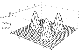
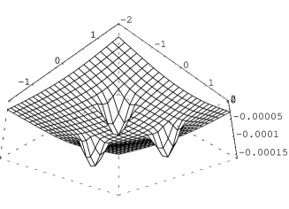
Figure 7: Condensates (left) and effective potential (right) on the $u$-plane for $m=0$, $f_{m}=0.14$.

For small values of the supersymmetry breaking parameter, the three BPS states condense around the corresponding singularities. This gives three degenerate minima spontaneously breaking the ${\bf Z}_{3}$ symmetry. They are located on the segments going from the three singularities to the origin of the $u$-plane, as required by the symmetry of the model. In fact they move away towards $u=0$, and for $f_{m}>0$ one has $|u|<1$ for the three minima. This generic situation is shown in fig. 7. It is important to notice that all the three states have an electric charge given by the effective theta angle through Witten’s effect. For the $(0,1)$ and $(1,1)$ states we have the same situation than in the dilaton spurion case: they have opposite electric charges. The $(2,1)$ state acquires an electric charge as the minimum moves towards the origin. We also have a nonzero squark condensate (2.13) at the minima which increases with $f_{m}$, as expected. The theory is then “Higgsed” as we turn on the mass spurion supersymmetry breaking parameter.

As in the previous cases, there is a maximum allowed value for $f_{m}\sim 1.4$, but before we reach this value a phase transition occurs: as the three minima approach each other they begin to overlap (as in [5]) and a new minimum develops at $u=0$. For $f_{m}\sim 0.93$ the minimum suddenly jumps to the origin and the ${\bf Z}_{3}$ symmetry is restored. There is there a simultaneous condensate of three mutually non-local states, which can be interpreted perhaps as a bound state with nonzero electric charge (in contrast to the bound state associated to two mutually non-local states). The electric charge of this object is associated to the $(2,1)$ state and would be $1/2$, while its magnetic charge would be $n_{m}=3$. This is a new different phase appearing in the softly broken $N=2$ QCD models.

  

Figure 8: Effective potential along the real $u$-axis for $m=0$ and $f_{m}=0.92$ (left) and $f_{m}=0.95$ (right).

Figure 9: The value of $|u|$ (vertical axis) at the minima as a function of $f_{m}$ (horizontal axis). The phase transition to $u=0$ takes place for $f_{m}\sim 0.93$.

This phase transition is clearly shown in fig. 8, where the effective potential is plotted along the real $u$-axis. One of the three degenerate minima (the one associated to the $(2,1)$ state) appears on the negative real axis. As $f_{m}$ passes through the critical value, the phase transition takes place and we are in the new phase with a minimum at $u=0$ and three simultaneous condensates. This is the phase we find until $f_{m}$ reaches the maximum allowed value. It is also illustrative to consider the evolution of $|u|$ at the minima as we turn on the supersymmetry breaking parameter $f_{m}$. This is plotted in fig. 9, where the sudden change in the position of the minimum is apparent.

3.4 The Phase Structure for $m$, $f_{m}$

The above picture changes when a real mass $m$ is introduced. As this explicitly breaks the ${\bf Z}_{3}$ symmetry, the only constraint on the dynamics of the theory comes from the CP symmetry. The mass term makes the $(2,1)$ minimum less favourable than the other two, and for small values of $m$, $f_{m}$ we have then two minima (associated to the $(0,1)$ and $(1,1)$ states) spontaneously breaking the CP symmetry. The situation is similar to the one found for the dilaton spurion breaking. As $f_{m}$ is increased, we have an overlapping of the condensates and a new minimum appears on the real $u$-axis with a first order phase transition, again similar to the one found for the dilaton spurion breaking. Indeed, it corresponds to two mutually non-local states condensing simultaneously (the $(0,1)$ and $(1,1)$ states).

  

Figure 10: Effective potential along the real $u$-axis for $m=0.1$ and $f_{m}=0.85$ (left) and $f_{m}=0.92$ (right).

As $f_{m}$ is still increased, the minimum moves smoothly along the real $u$-axis to the origin. At a certain point, the $(2,1)$ condensate is different from zero at the minimum and we have again a phase with three condensates, like the one we found for $m=0$. There are then two smoothly connected phases but with a different number of condensates at the minimum. This is shown in fig. 10, where the effective potential is plotted on the real $u$ axis for $m=0.1$ and $f_{m}=0.85$, $0.92$. In the first case the minimum has $\rho=0$ for the $(2,1)$ condensate, while $\rho\not=0$ in the second case. In fact, the $(2,1)$ condensate can be considered as a continuous order parameter for this transition. The minimum moves smoothly to the origin along the real $u$ axis as $f_{m}$ is increased.

The “window” in which we have the phase with a condensate of two mutually non-local states becomes bigger as $m$ is increased. For a certain value of $m$ this is the only non-local phase we find, as the singularity corresponding to the $(2,1)$ state moves away from the origin of the $u$-plane. The new phase with three mutually non-local states dissapears, and the situation is essentially similar to the one we found for the dilaton spurion induced supersymmetry breaking. The maximum allowed value for $f_{m}$ also decreases as we approach the Argyres-Douglas point, and $m=m_{c}$ is also a critical value for the mass in this model. The vacuum structure completely changes for $m>m_{c}$. What we find there is a single minimum on the real $u$ axis corresponding to a quark condensate. At this minimum there is a nonzero VEV for ${\tilde{q}}q$, as expected.

Figure 11: Effective potential along the real $u$ axis for $m=2$, $f_{m}=0.56$.

The $(2,1)$ dyon condensate is also different from zero, but smaller than the quark condensate in one order of magnitude. Finally, the monopole hardly condenses and in fact the cosmological constant is smooth at the monopole singularity. It is interesting to notice that, in the decoupling limit, the vacuum moves away to infinity together with the quark singularity. We have then a “runaway vacua”-like phenomenon. This is expected, as the terms that lift the vacuum degeneracy of the $N=2$ supersymmetric theory in the bare Lagrangian are off-diagonal mass terms for the squarks, and when the quark hypermutliplet is decoupled they do not longer affect the $N=2$ vacuum structure. The whole $u$-plane of vacua is recovered.

The situation is illustrated in fig. 11, where the effective potential is plotted along the real $u$-axis for $m=2$, $f_{m}=0.56$. The absolute minimum occurs around the quark singularity at $u\sim 4.2$. There is also a relative minimum around the $(2,1)$ dyon singularity $u\sim-2.6$.

Figure 12: Phase structure of the $N_{f}=1$ theory for $m$, $f_{m}$ (denoted as Fm).

The phases and vacuum structure when we turn on $m$, $f_{m}$, are summarized in fig. 12. Again there are two different behaviours, depending on wether $m<m_{c}$ or $m>m_{c}$. When $m<m_{c}$, $m\not=0$, there are three different phases for small values of $m$. The first one has two minima with dyon condensation and is separated from the second one (denoted by “non local I”) by a first order phase transition. This non-local phase exhibits simultaneous condensation of the $(0,1)$ and $(1,1)$ states, and is smoothly connected to a third phase (“non-local II” in the diagram) where there is also a condensate of the $(2,1)$ state. As $m$ increases, the third phase disappears, and as $m$ approaches $m_{c}$ from below the second phase also does (as in the dilaton spurion case). When $m>m_{c}$, the theory is in a different phase, and the vacuum corresponds to an elementary quark condensate.

4 $N_{f}=2$ Vacuum Structure

In this section we analyse the vacuum structure of softly broken $N=2$ QCD with two massive quark hypermultiplets. We focus on the new physical phenomena arising because of the non abelian flavor group. In the first subsection the relevant symmetries are presented and the vacuum equations are solved for general spurions. In the second subsection we study the case of breaking only with dilaton spurion. In the next two subsections we discuss the phase transitions produced by the combination of mass and dilaton spurions.

4.1 Symmetries and Monopole Condensates

With $N=2$ supersymmetry, the superpotential links the flavor rotations of the left handed quarks and antiquarks. For $SU(2)$ gauge group, since the fundamental representation is pseudoreal, we can arrange the $N_{f}$ flavors in a vectorial representation of $SO(2N_{f})$.

For $N_{f}=2$ massless hypermultiplets, the global flavor symmetry group is $SO(4)$. Let us study more closely how the bare quark masses explicitly break the flavor group. The mass term can be written with the $4\times 4$ antisymmetric matrix $V^{rs}=Q^{r}Q^{s}$ in the ${\bf 6}$ representation of $so(4)$. In terms of its selfdual and anti-sefldual parts, $V^{rs}=V^{rs}_{+}+V^{rs}_{-}$, the flavor group representation is $({\bf 3,1})\oplus({\bf 1,3})$ of $so(4)=su(2)_{-}\oplus su(2)_{+}$, respectively. The mass term turns out to be

$$\sum_{f=1}^{2}m_{f}{\tilde{Q}}^{f}Q^{f}=2im_{+}V_{-}^{13}+2im_{-}V_{+}^{13}.$$ (4.1)

$m_{\mp}=m_{1}\mp m_{2}$ are the breaking parameters of the flavor subgroups $SU(2)_{\mp}$, respectively. Such variables are more adequate for the analysis of the $N_{f}=2$ massive theory. For $m_{\mp}=0$, the moduli space of the Coulomb branch of the theory has a singularity at $u=\pm 1$, where a doublet of magnetic BPS states in the $({\bf 2,1})$ or $({\bf 1,2})$ flavor representations, respectively, become massless. ¿From these points a Higgs-confining branch emerges with one real modulus given by $<V_{\pm}>\not=0$ and $<V_{\mp}>=0$, for $u=\pm 1$, respectively.

Figure 13: The singularities of the $u$-plane for real bare masses $m_{\pm}$.    Figure 14: Plot of the supersymmetric BPS masses of the two light monopoles M1 and M2 along the path joining the complex conjugate splitted singularities for $m_{\pm}=1/3$.

If we turn on the bare parameter $m_{\mp}$, the singularity at $u=\pm 1$ splits in two singularities with a single massless state, showing the explicit breaking of the $SU(2)_{\mp}$ flavor subgroup in the bare Lagrangian (see fig. 13). The BPS masses of the two light magnetic hypermultiplets also split because of the different baryon numbers of the unbroken $U(1)_{\mp}\subset SU(2)_{\mp}$ symmetry (see fig. 14). For $N_{f}=1$ we could make a local inhomogeneous duality transformation on a given vanishing cycle such that it does not enclose any simple pole of $\lambda_{SW}$, giving baryon number equal to zero to the associated BPS state. But for $N_{f}=2$ there are two mutually local singularities. We can choose one of them to have baryon numbers equal to zero, but that fixes unambiguously the baryon numbers of the other one. It is the quantity $S^{\mp}_{2}-S^{\mp}_{1}$ which has a duality invariant meaning and carries all the information we need about the baryon numbers. For quark baryon numbers normalized to one, we have $S^{\mp}_{2}-S^{\mp}_{1}=1$ and $S^{\pm}_{2}-S^{\pm}_{1}=0$ for the region around $u=\pm 1$, respectively.

Then, for $N_{f}=2$ massive softly broken $N=2$ QCD, we have two well differentiated regions: the monopole region near $u=1$ and the dyon region near $u=-1$. In these regions, the relevant degrees of freedom at low energies are an $U(1)_{G}$ abelian vector multiplet and two light charged hypermultiplets. The soft $N=2$ supersymmetry breaking terms generate a non trivial effective potential for each region. The analysis becomes more clear if we capture the symmetries broken by the small perturbations. We define the $2\times 2$ matrix

$$\Phi^{ia}=\left(\matrix{h_{1}&{\bar{\tilde{h}}}_{1}\cr h_{2}&{\bar{\tilde{h}}}_{2}}\right)$$ (4.2)

in the $({\bf 2},{\bf 2},0,1)$ representation of $SU(2)_{\mp}\times SU(2)_{R}\times U(1)_{R}\times U(1)_{G}$, for the monopole or dyon region, respectively. The action of the global symmetries is

$$\Phi^{ia}\rightarrow g_{\mp}^{ij}\Phi^{jb}(g^{\dagger}_{R})^{ba}.$$ (4.3)

The supersymmetry breaking parameters, as auxiliary terms of the $N=2$ spurion fields, can be thought as frozen vectors in the adjoint of $SU(2)_{R}$. They can be written as a unitary $2\times 2$ matrix:

$${\bf F}^{A}=\left(\matrix{D^{A}&{\sqrt{2}}F^{A}\cr{\sqrt{2}}\,{\overline{F}}^{A}&-D^{A}}\right)={\sqrt{2}}{\rm Re}[F^{A}]\sigma^{1}-{\sqrt{2}}{\rm Im}[F^{A}]\sigma^{2}+D^{A}\sigma^{3},$$ (4.4)

where $A=0,+,-$.

The supersymmetric BPS masses of the two light hypermultiplets can be thought as frozen vectors in the adjoint of the $SU(2)_{\mp}$:

$${\bf M}=\left(\matrix{|{\sqrt{2}}a+S^{f}_{1}m_{f}|&0\cr 0&|{\sqrt{2}}a+S^{f}_{2}m_{f}|}\right).$$ (4.5)

The effective potential is

$$V_{{\rm eff}} = {1\over 4}B_{AB}{\rm Tr}\{{\bf F^{A}}{\bf F^{B}}\}+{1\over 2b_{aa}}\left(2{\rm Tr}\{(\Phi\Phi^{\dagger})^{2}\}-({\rm Tr}\{\Phi\Phi^{\dagger}\})^{2}\right)$$ (4.6)

$$+ {\rm Tr}\{{\bf M}^{2}\Phi\Phi^{\dagger}\}+{1\over b_{aa}}{\rm Tr}\{\Phi(b_{aA}{\bf F}^{A})\Phi^{\dagger}\}$$

$$- \sum_{i=1}^{2}S^{f}_{i}\Phi^{ia}{\bf F}_{f}^{ab}(\Phi^{\dagger})^{bi}.$$

The first term corresponds to the cosmological constant, where each of the six factors $B_{AB}=({b_{aA}b_{aa}^{-1}b_{aB}}-b_{AB})$ is duality invariant (I). The second term is $SU(2)_{\mp}\times SU(2)_{R}$ invariant. The third term breaks $SU(2)_{\mp}$ explicitly and is $SU(2)_{R}$ invariant. The fourth term breaks $SU(2)_{R}$ explicitly and is $SU(2)_{\mp}$ invariant. The fifth term breaks $SU(2)_{\mp}$ and $SU(2)_{R}$ simultaneously. In the bare Lagrangian, $m_{f}$ and/or $F_{f}$ different from zero break $SO(4)\rightarrow SO(2)_{1}\times SO(2)_{2}$. But at the level of the vacuum structure, as the monopoles (dyons) do not carry the quantum numbers of $SU(2)_{+(-)}$, the effect at low energy of the $SU(2)_{\mp}$ breakings is only seen on the monopoles and dyons effective potentials, respectively. Finally, we observe that for each local effective potential, the $SU(2)_{\mp}$ breaking terms are still invariant under an abelian subgroup $U(1)_{\mp}\subset SU(2)_{\mp}$. Also, if we only break supersymmetry with the dilaton spurion, there is an unbroken $U(1)\subset SU(2)_{R}$ given by the direction of the vector ${\bf F}_{0}$.

Next we focus on the vacuum structure. We first solve for the minimum of the effective potential in terms of the monopole condensates for a given vacuum $u$. As in the previous section, we consider the case of supersymmetry breaking purely by $F$-terms, i.e., we put $D^{A}=0$ for all spurions, being the difference only an $SU(2)_{R}$ rotation of the monopole condensate solutions. The equations are

$${\partial V_{{\rm eff}}\over\partial{\bar{h}}_{i}}={1\over b_{aa}}(|h|^{2}-|{\tilde{h}}|^{2})h_{i}+{2\over b_{aa}}({\tilde{h}}h){\bar{\tilde{h}}}_{i}$$

$$+|{\sqrt{2}}a_{i}|^{2}h_{i}+{{\sqrt{2}}\over b_{aa}}{\overline{F}}_{i}{\bar{\tilde{h}}}_{i}=0,$$ (4.7)

$${\partial V_{{\rm eff}}\over\partial{\bar{\tilde{h}}}_{i}}={-1\over b_{aa}}(|h|^{2}-|{\tilde{h}}|^{2}){\tilde{h}}_{i}+{2\over b_{aa}}({\tilde{h}}h){\bar{\tilde{h}}}_{i}$$

$$+|{\sqrt{2}}a_{i}|^{2}{\tilde{h}}_{i}+{{\sqrt{2}}\over b_{aa}}{\overline{F}}_{i}{\bar{h}}_{i}=0,$$ (4.8)

where, to simplify notation, we have defined

$$|h|^{2}=\sum_{i=1}^{2}|h_{i}|^{2},\quad\quad{\tilde{h}}h=\sum_{i=1}^{2}{\tilde{h}}_{i}h_{i},$$

$$a_{i}=a+S^{f}_{i}{m_{f}\over{\sqrt{2}}},\quad\quad F_{i}=b_{aA}F^{A}-b_{aa}S^{f}_{i}F_{f}.$$ (4.9)

If we consider the combination

$${\bar{h}}_{i}{\partial V_{{\rm eff}}\over\partial{\bar{h}}_{i}}-{\bar{\tilde{h}}}_{i}{\partial V_{{\rm eff}}\over\partial{\bar{\tilde{h}}}_{i}}=0$$ (4.10)

we obtain a linear sistem of homogeneous equations for the variable $(|h_{i}|^{2}-|{\tilde{h}}_{i}|^{2})$ with determinant different from zero. This implies that $|h_{i}|=|{\tilde{h}}_{i}|$, for each $i=1,2$, a consequence of breaking only with $F$-terms. We make the parametrization $h_{i}=\rho_{i}e^{i\beta_{i}}$ and ${\tilde{h}}_{i}=\rho_{i}e^{i{\tilde{\beta}}_{i}}$, to obtain the vacuum equations

$$\rho_{i}\left(\sum_{j=1}^{2}(\rho_{j}^{2}e^{i(\beta_{j}+{\tilde{\beta}}_{j})})+b_{aa}|a_{i}|^{2}e^{i(\beta_{i}+{\tilde{\beta}}_{i})}+{{\overline{F}}_{i}\over{\sqrt{2}}}\right)=0.$$ (4.11)

If $\rho_{i}\not=0$ for all $i=1,2$, subtracting both equations (4.11) we obtain the compatibility equation

$$|a_{2}|^{2}e^{i(\beta_{2}+{\tilde{\beta}}_{2})}-|a_{1}|^{2}e^{i(\beta_{1}+{\tilde{\beta}}_{1})}={{\overline{F}}_{\mp}\over{\sqrt{2}}}$$ (4.12)

near $u=\pm 1$, respectively. If (4.12) is not satisfied, then we cannot have simultaneous condensation of the mutually local monopoles. The solution is

$$\rho_{i} = -b_{aa}|a_{i}|^{2}+{|{\overline{F}}_{i}|\over{\sqrt{2}}},$$ (4.13)

$$\beta_{i}+{\tilde{\beta}_{i}} = {\rm Arg}[{\overline{F}}_{i}]+\pi,$$ (4.14)

$$\rho_{j} = 0\quad\quad(j\not=i).$$ (4.15)

If we introduce the monopole condensate into the effective potential, we obtain the $u$ dependent function

$$V_{{\rm eff}}(u)=B_{AB}(u){\overline{F}}^{A}F^{B}-{2\over b_{aa}(u)}\rho^{4}(u).$$ (4.16)

with $\rho={\rm Max}[\rho_{1},\rho_{2}]$, the bigger condensate which minimizes the vacuum energy. As the monopoles have different baryon numbers, the potential is anisotropic. There are different prefered directions for the vector $(\rho_{1},\rho_{2})$ depending on the region of the moduli space. At the transition point $\rho_{1}=\rho_{2}$ there is a flip in the VEV direction which produces a discontinuous first derivative of $V_{{\rm eff}}(u)$. This cusp in the effective potential shows a first order phase transition associated to the level crossing of the $\rho_{1}$ and $\rho_{2}$ condensates: on the cusp line, the configuration minimizing the vacuum energy changes from one direction to the other, i.e., from the energy level given by the $\rho_{1}$ VEV to the one given by the $\rho_{2}$. We expect to smooth this cusp if the next to leading contributions to the effective potential are included.

4.2 Breaking with only Dilaton Spurion

  

Figure 15: Plot of the $|F_{0}|^{2}$ cosmological constant factor $B_{00}(u)$ through the path which joins the two mutually local singularities in the monopole region (left) and in the dyon region (right) for $m_{\pm}=1/3$.

In this subsection we focus on the vacuum structure originated by the supersymmetry breaking only with $F_{0}\not=0$, putting mass spurions $F_{f}=0$. The massless case was studied in [4]. In the numerical analysis we choose the normalization $\Lambda^{2}_{2}=8$.

The order parameter which makes possible the monopole condensate is the coupling $b_{a0}$. As in the massless case, it is practically zero near the dyon region, with a cosmological constant already smooth at $u\sim-1$ (see fig. cosmdilaton, right). The dilaton parameter explicitly breaks the ${\bf Z}^{R}_{2}\subset U(1)_{R}$ symmetry and the minimum is located at the monopole region $u\sim 1$.

For real bare quark masses, the supersymmetry breaking order parameter $b_{a0}$ and the cosmological constant are symmetric with respect to the CP action $u\rightarrow{\bar{u}}$ (see fig. 15, left). When we include the monopole condensate contribution to the effective potential we obtain two smooth minima near the two splitted monopole singularities. These two minima are energetically degenerate, located at complex conjugate points in the $u$-plane. There is an spontaneous symmetry breaking of the CP symmetry. The states condensing at these vacua have opposite physical electric charges $q(u)=\theta_{{\rm eff}}(u)/\pi\not=0$, induced by Witten’s effect [10].

If we give complex phases $m_{\mp}\rightarrow e^{i\alpha_{\mp}}m_{\mp}$ to the bare masses, the $u$ singularities rotate around $u=\pm 1$, respectively. If their phase is the same, we can perform an $U(1)_{R}$ anomalous transformation to absorb the common global phase into the bare $\theta$ angle. This corresponds to a rotation of the $u$-plane [6], and we obtain the same physical situation. But if the bare quark masses have a relative complex phase, the CP symmetry is lost and we only have one absolute minimum, which is always located at the singularity with the biggest value for $|u|$.

The cusp line is on the points of the $u$-plane where the two monopoles have the same mass, which for real bare quark masses is on the real $u$-axis (see fig. 14).

Figure 16: The monopole condensate $\rho={\rm Max}[\rho_{1},\rho_{2}]$ for $f_{0}=1/10$ and $m_{\pm}=1/3$.    Figure 17: The effective potential in the monopole region for $f_{0}=1/10$ and $m_{\pm}=1/3$.

The cusp appears when the two condensates start to overlap, for values of the dilaton spurion bigger than some critical value $F_{0}^{(c)}(m_{-})$ (See fig. 16 and fig. 17).

4.3 Breaking with Mass Spurions: Phase Transitions between Mutually Local Minima

When we turn on the mass spurion supersymmetry breaking parameters, a rich phase structure emerges. The first thing to notice is that when $|F_{-}|$ or $|F_{+}|$ are increased, the absolute minimum tends to be in the monopole or dyon region, respectively. We will study these phenomena in the next subsection. In this subsection we shall consider that there is still a value of $F_{0}$ large enough for the absolute minimum to be in the $u\sim 1$ region, and focus on the phase transitions between the minima associated to mutually local singularities.

    

Figure 18: The supersymmetry breaking mass couplings $b_{a-}^{(1)}$ (left), $b_{a-}^{(2)}$ (middle) and $b_{a+}$ (right) along the path joining the complex conjugate monopole $u$-singularities for $m_{\pm}=1/3$.

When we turn on the mass spurions, we must be careful with the monopole condensates $\rho_{i}$. We have seen that the vacuum chooses the biggest local condensate $\rho={\rm Max}[\rho_{1},\rho_{2}]$. If one breaks supersymmetry with only the dilaton spurion, the functions $\rho_{i}$ (4.13) go to zero on the $u_{j}$ ($j\not=i$), and for each singularity, the vacuum chooses always its corresponding local condensate. We can take the massless limit keeping $F_{0}$ different from zero, and then we recover the situation described in [4]. At the same time, the cusp disappears as the flavor symmetry is restored. But when we turn on the mass spurions, their contribution to the $\rho_{i}$ condensate is proportional to $b_{a-}^{(i)}=b_{a+}F_{+}+(b_{a-}-b_{aa}S_{i}^{-})F_{-}$. This is the adequate coupling near the $u_{i}$ singularity, as it corresponds to the right local variable there, $a_{i}=a+S_{i}^{-}m_{-}/{\sqrt{2}}$. This coupling does not diverge at $u_{i}$.

  

Figure 19: The cosmological constant factors $B_{0-}$ (left) and $B_{++}$ (right) along the path joining the complex conjugate monopole singularities for $m_{\pm}=1/3$.

But then it will inevitably diverge at the other mutually local $u_{j}$ singularity ($j\not=i$) (see fig. 18). To avoid this divergence, the $\rho_{i}$ condensate must not attain the $u_{j}$ singularity, and this condition will give an upper bound for the mass spurions. Let us consider the condensate $\rho_{2}$ in terms of the $a_{1}$ variable, which has the baryon numbers $(S^{+}_{2},S^{-}_{2})=(0,1)$. We can redefine the monopole phases such that $F_{-}$ is real and positive, and then we expand in powers of $1/(b_{aa}F_{-})$:

$$\rho_{2} = b_{aa}\left(F_{-}-{1\over{\sqrt{2}}}|{\sqrt{2}}a_{1}+m_{-}|^{2}\right)$$ (4.17)

$$- {1\over{\sqrt{2}}}{\rm Re}[b_{a0}F_{0}++b_{a+}F_{+}+b_{a-}^{(1)}F_{-}]+{\cal O}({1\over b_{aa}F_{-}}),$$

which goes to infinity at $u_{1}$ for $F_{-}>|m_{-}|^{2}/{\sqrt{2}}$. The $b_{a+}$ coupling, as the monopoles do not have $SU(2)_{+}$ quantum numbers, remains finite at both singularities (see fig. 18, right). Actually, its contribution to the condensate is two orders of magnitude smaller than the one associated to the $b_{a-}^{(i)}$ couplings.

Then, if we do not want the monopole and dyon condensates to explode at the other mutually local singularities, we must impose the upper bounds $F_{\pm}^{(Max)}=|m_{\pm}|^{2}/{\sqrt{2}}$ to the mass supersymmetry breaking parameters. In the massless limit, $m_{f}\rightarrow 0$, we must also send the mass spurions to zero. This indicates that for mass spurions bigger than these bounds, the effective potential is unbounded from below. This instability of the vacuum is expected from the structure of the soft breaking terms in the bare Lagrangian, as we already mentioned in section 2.

  

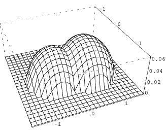
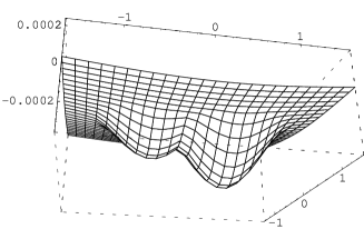
Figure 20: The monopole condensate (left) and the effective potential (right) for $F_{0}=1/10$ and $F_{-}=-{1\over 5}F^{max}_{-}$.

For real bare masses, the cosmological constant factors $B_{0\mp}(u)$ and the couplings $b_{a-}^{(i)}$ and $b_{a+}$ are antisymmetric with respect to the CP action (see fig. 19 (left) and fig. 18). Then, for two generic spurions different from zero, there is a first order phase transition between local minima, as we change the sign of their relative phase. To be concrete, take $F_{0}$ and $F_{-}$ to be real numbers. When they have the same sign, the $\rho_{1}$ condensate is bigger than the $\rho_{2}$ condensate. Also, the effective potential has the absolute minimum near $u_{1}$. When the spurions have opposite signs, we obtain the CP transformed situation, and now the absolute minimum is near $u_{2}$ (see fig. 20). The CP symmetry is explicitly broken in the effective potential.

4.4 Breaking with Mass Spurions: Phase Transitions between Mutually Non-Local Minima

When we decrease $|F_{0}|$ with respect to $|F_{\pm}|$, the dyon region enters the game. For real bare masses, the cosmological constant factor $B_{--}$ looks like the factor $B_{00}$ in the monopole and dyon regions (see fig. 15). In the dyon region, $B_{++}$ is like $B_{--}$ in the monopole region and the supersymmetry breaking couplings $b_{a+}^{(i)}$ are of the same order of magnitude as the $b_{a-}^{(i)}$ couplings in the monopole region. For $|F_{+}|>|F_{-}|$, if we decrease $|F_{0}|$, the effective potential in the monopole region is dominated by the smooth cosmological constant factor $B_{++}$ (see fig. 19, left). There is a critical value of the dilaton spurion for which the absolute minimum jumps to the dyon region, and we have a first order phase transition between mutually non-local minima, which have different patters of chiral symmetry breaking.

For $F_{0}=0$, the ${\bf Z}^{R}_{2}$ symmetry in the bare Lagrangian is only broken by the bare quark masses. If we take complex conjugate masses, $m_{1}={\overline{m}}_{2}$, the M1 and M2 monopole singularities (see fig. 13) rotate counterclockwise and all the singularities of the $u$-plane are on the real axis. It is only in this extreme situation that there is a complete symmetry between the monopole and dyon region, if we also interchange the variables with indices $+$ and $-$. From now on we will consider this symmetric situation.

For $|F_{-}|>|F_{+}|$, the absolute minimum is in the monopole region. When their relative phase changes sign, there is a first order phase transition between the two monopole minima, as the one plotted in fig. 20. Across the lines $|F_{+}|=|F_{-}|$ there is a first order phase transition between the mutually non-local minima. These minima give different realizations of the chiral symmetry breaking pattern, and we have $SU(2)_{-}\times SU(2)_{+}\rightarrow SU(2)_{\pm}$ for the monopole and dyon regions, respectively.

  

Figure 21: The non-local first order phase transition for $m_{1}={\bar{m}_{2}}={7\over 10}(1+i)$ and $F_{-}=F_{+}=0.15F_{\pm}^{Max}$.

If we simultaneously increase $|m_{+}|$ and $|m_{-}|$, the monopole and dyon singularities which are nearest to the origin approach each other, and they meet at the superconformal AD $(1,1)$ point at $u=0$ for $m_{+}=1$ and $m_{-}=i$ [9]. But before that happens, the monopole and dyon condensates begin to overlap. For a critical value of the bare quark masses ($|m_{\pm}|\sim 7/10$), this overlaping gives rise to a new minimum at $u=0$, provided that the supersymmetry breaking parameters are large enough (see fig. 21). Once again, we find a first order phase transition similar to the ones considered in [5] and in the previous section. Both states have opposite physical electric charges at $u=0$, and we also observe in this case the possibility of the formation of an electrically neutral “bound state” at $u=0$. We then see that these kinds of phenomena are generic in the $N=2$ softly broken models. The interesting thing of the $N_{f}=2$ case is that this “bound state” is made of mutually non-local states with different flavor quantum numbers. The monopole is in the flavor representation $({\bf 2,1})$ and the dyon in the $({\bf 1,2})$ of the $SU(2)_{-}\times SU(2)_{+}$ flavor group. The formation of this bound state could be a hint that the new absolute minimum breaks $SU(2)_{+}\times SU(2)_{-}$ to the diagonal $SU(2)_{V}$.

Figure 22: Phase diagram with $F_{0}=0$ and $m_{1}={\bar{m}_{2}}\approx{7\over 10}(1+i)$ to have the M2 + D2 phase. M2 means a vacuum dominated by the condensate of the monopole nearest to $u=0$. D2 means the same thing, but for the dyon. M1 and D1 are the other more distant singularities.

Finally, in fig. 22 we give the phase diagram of $N_{f}=2$ massive softly broken $N=2$ QCD, for dilaton spurion $F_{0}=0$ and complex conjugate bare quark masses with modulus bigger than the critical value needed to see the phase transition at $u=0$. The corners labeled by M2 + D2 correspond to this new phase. To symplify, the mass spurions are taken to be real. There are first order phase transitions between mutually local minima when their relative sign changes, i.e., across the $F_{\mp}$ axis. There are also first order phase transitions across the diagonals $|F_{-}|=|F_{+}|$, where the absolute minima jumps between the monopole and dyon regions. For given values of the bare masses, there are maximum allowed values for the mass spurions. This is why the phase diagram is enclosed into an square box, in such a way that none of the condensates reaches another singularity.

If we compute the squark condensates $<{\tilde{q}}_{f}q_{f}>$ given in (2.13) at the minimum, for the massless case, we can check that $<V_{+}>\not=0$ and $<V_{-}>=0$. This is consistent with the spontaneous symmetry breaking of the $SU(2)_{-}$ flavor subgroup due to the VEV of the monopole doublet. In the following section we give the pion Lagrangian associated to this spontaneous symmetry breaking.

5 The Pion Lagrangian

One of the main features of the Seiberg-Witten solution in [3] is that chiral symmetry breaking is naturally explained in terms of monopole condensation, once $N=2$ supersymmetry is broken down to $N=1$ [3] or to $N=0$ [4]. As we also have a low-energy effective Lagrangian describing the dynamics of the monopoles, one can try to obtain the “pion” Lagrangian up to two derivatives for the Goldstone bosons associated to the chiral symmetry breaking. This provides an interesting information about the dependence of phenomenological parameters like the pion mass and $F_{\pi}$ in terms of the magnetic monopole description. Although the pattern of chiral symmetry breaking in the softly broken models is not completely QCD-like, certain aspects of this analysis could be of interest in more realistic models.

When we soflty break supersymmetry down to $N=0$ with only a dilaton spurion in the $N_{f}=2$ theory with massless hypermultiplets, the flavor symmetry is not explicitly broken, and the minimum is located in the monopole region. Near the monopole singularity, the global symmetry of the model is $G=SU(2)_{-}\times U(1)$. The $U(1)\subset SU(2)_{R}$ corresponds to the unbroken subgroup given by the direction of the $SU(2)_{R}$ vector, ${\bf F}_{0}$. This will be our chiral symmetry group. For real and positive $F_{0}=f_{0}$ and $D_{0}=0$, the unbroken $U(1)$ can be parametrized by a $\theta$ angle as $g_{1}={\rm exp}(-i\sigma_{1}\theta)$. We parametrize $SU(2)_{-}$ in the standard way as $g_{-}={\rm exp}(-i{\bf\theta}\cdot{\bf\sigma})$, where ${\bf\theta}=(\theta_{1},\theta_{2},\theta_{3})$ and ${\bf\sigma}$ are the Pauli matrices. The monopole VEV spontaneously breaks $G=SU(2)_{-}\times U(1)$ down to an $H\simeq U(1)$ subgroup. To obtain the precise form of the symmetry breaking pattern, we choose a minimum with $h_{1}\not=0$, $h_{2}=0$. We then have

$$\Phi_{0}=\left(\begin{array}[]{cc}\rho&\epsilon\rho\\ 0&0\end{array}\right),$$ (5.1)

where $\epsilon=-b_{a0}/|b_{a0}|$ is the phase of ${\tilde{h}}_{1}$. The unbroken group $H$ corresponding to the minimum in (5.1) is then generated by $\theta_{1}=\theta_{2}=0$ and $\theta=\epsilon\theta_{3}$. The vacua associated to the coset space $G/H$ can be parametrized as

$$\Phi({\bf\theta})={\rm e}^{-i{\bf\theta}\cdot{\bf\sigma}}\Phi_{0}{\rm e}^{-i\epsilon\theta_{3}\sigma_{1}},$$ (5.2)

The three parameters in $\theta$ correspond to the three Goldstone bosons of the spontaneously broken $G$-symmetry. We will now derive the effective Lagrangian up to two derivatives describing them, once the bare mass terms and the mass spurions terms are introduced. These terms explicitly break the $SU(2)_{-}\times U(1)$ symmetry, and if they are small we can also compute exactly the induced masses for the Goldstone bosons [18]. The effective potential with the explicit breaking terms will have now a dependence on the $\theta$ angles, and we must find the minimum of $V_{\rm eff}$ in the $G/H$ space. We can write

$$V_{{\rm eff}}=V_{0}+{\rm Tr}\{{\bf M}^{2}\Phi\Phi^{\dagger}\}-\sum_{i=1}^{2}S_{i}^{f}\Phi^{ia}{\bf F}_{f}^{ab}(\Phi^{\dagger})^{bi},$$ (5.3)

where we have denoted by $V_{0}$ the $SU(2)_{-}\times U(1)$ symmetry-preserving terms, and the ${\Phi}$ matrix is the $\theta$-dependent one in (5.2). After some straightforward algebra we obtain:

$$V_{\rm eff}(\theta) = V_{0}+2\rho^{2}\{2|a_{1}|^{2}-{\sqrt{2}}\epsilon S_{1}^{f}{\rm Re}\,[F^{f}]\}$$ (5.4)

$$+ 2\rho^{2}(1-{\hat{\theta}_{3}}^{2}){\rm sin}^{2}|\theta|\{2(|a_{2}|^{2}-|a_{1}|^{2})-{\sqrt{2}}\epsilon{\rm Re}\,[F_{-}]\},$$

where $|\theta|=(\theta_{1}^{2}+\theta_{2}^{2}+\theta_{3}^{2})^{1/2}$, and ${\hat{\theta}_{i}}=\theta_{i}/|\theta|$, $i=1,2,3$. There are two different minima, depending on the sign of the term multiplying $(1-{\hat{\theta}_{3}}^{2}){\rm sin}^{2}|\theta|$.

1) If $2(|a_{2}|^{2}-|a_{1}|^{2})-{\sqrt{2}}\epsilon{\rm Re}\,[F_{-}]>0$, the minimum is located at $\theta_{1}=\theta_{2}=0$ and $\theta_{3}$ arbitrary. We then see that one of the directions in $G/H$ remains flat, therefore one of the pions will remain massless. This is a consequence of the fact that the terms explicitly breaking $SU(2)_{-}$ in (5.3) still leave an unbroken $U(1)_{-}\subset SU(2)_{-}$. If we consider small fluctuations around this minimum, it is natural to expand also around $\theta_{3}=0$, and we have then at first order

$$\Phi(\theta)=(1-i{\bf\sigma}\cdot{\bf\xi})\Phi(\theta_{*}),$$ (5.5)

where $\theta_{*}=(0,0,0)$. The ${\xi}$-variables are given by

$$\xi_{1}=\theta_{1},\,\,\,\ \xi_{2}=\theta_{2},\,\,\,\ \xi_{3}=2\theta_{3}.$$ (5.6)

The potential (5.4) can also be expanded to obtain

$$V_{\rm eff} = V_{0}+2\rho^{2}\{|a_{1}|^{2}-{\sqrt{2}}\epsilon S_{1}^{f}{\rm Re}\,[F^{f}]\}$$ (5.7)

$$+ 2\rho^{2}\{2(|a_{2}|^{2}-|a_{1}|^{2})-{\sqrt{2}}\epsilon{\rm Re}\,[F_{-}]\}(\xi_{1}^{2}+\xi_{2}^{2}),$$

To identify the pion fields ${\pi}_{i}$, $i=1,2,3$, we require the standard normalization for the kinetic terms,

$${\rm Tr}\{{\partial_{\mu}}\Phi{\partial^{\mu}}{\Phi^{\dagger}}\}={1\over 2}\sum_{i=1}^{3}{\partial_{\mu}}\pi_{i}{\partial^{\mu}}\pi_{i},$$ (5.8)

which leads to

$$\pi_{i}=2\rho\xi_{i},\,\,\,\,\,\ i=1,2,3.$$ (5.9)

From (5.7) and (5.9) we finally obtain the pion mass and $F_{\pi}$ as

$$M^{2}_{\pi_{1}}=M^{2}_{\pi_{2}}=2(|a_{2}|^{2}-|a_{1}|^{2})-{\sqrt{2}}\epsilon{\rm Re}\,[F_{-}],\,\,\,\,\,\ M^{2}_{\pi_{3}}=0,$$

$$F_{\pi}=2\rho,$$ (5.10)

and we see that, indeed, one of the pions will remain massless.

2) If $2(|a_{2}|^{2}-|a_{1}|^{2})-{\sqrt{2}}\epsilon{\rm Re}\,[F_{-}]<0$, the minimum is located at $\theta_{3}=0$, $|\theta|=\pi/2$. We then parametrize

$$\theta_{1}=\Big{(}{\pi\over 2}+r\Big{)}{\rm sin}\phi,\,\,\,\,\,\,\theta_{2}=\Big{(}{\pi\over 2}+r\Big{)}{\rm cos}\phi,$$ (5.11)

so that the minimum occurs at $\theta_{3}=r=0$ and $\phi$ arbitrary. Again there is a flat direction and a massless pion. We consider small fluctuations around $(r,\phi,\theta_{3})=(0,0,0)$, i.e., $\theta_{*}=(0,\pi/2,0)$, and obtain

$$\xi_{1}={2\over\pi}\theta_{3},\,\,\,\ \xi_{2}=r,\,\,\,\ \xi_{3}=-(\phi+\theta_{3}).$$ (5.12)

Notice that $\Phi(\theta_{*})$ corresponds, for the minimum considered in (1), to a monopole VEV in the $h_{1}$ direction, and for the minimum considered here, to a VEV in the $h_{2}$ direction. These two different cases clearly show the anisotropy in the VEV direction once $SU(2)_{-}$ terms are introduced, as one direction or another is favoured depending on the value of $2(|a_{2}|^{2}-|a_{1}|^{2})-{\sqrt{2}}\epsilon{\rm Re}\,[F_{-}]$. As we are restricting the $\Phi$ values to $G/H$ configurations, the conditions to have one VEV direction or the other will only agree with the ones derived in section 4 in the case $F_{f}=0$ (as in this case the exact solution is in $G/H$).

Once we have found the appropriate $\xi_{i}$ parameters, we can follow the procedure in (1) and we arrive to the same $F_{\pi}$ and to the same mass spectrum: one of the pions remains massless and for the other two we have the same result as in (5.10) but with the opposite sign (in such a way that the squared mass is always positive).

In both minima we have then the same physical situation, which we can summarize as:

$$M^{2}_{\pi_{1}}=M^{2}_{\pi_{2}}=|2(|a_{2}|^{2}-|a_{1}|^{2})-{\sqrt{2}}\epsilon{\rm Re}\,[F_{-}]|,\,\,\,\,\,\ M^{2}_{\pi_{3}}=0,$$

$$F_{\pi}=2\rho.$$ (5.13)

The physical meaning of these equations is very appealing. They are telling us that, if chiral symmetry is broken by magnetic monopole condensation, then $F_{\pi}$ is given by the VEV of the monopole. Also notice that, for $F_{-}=0$, the pion mass is simply given by the difference between the BPS masses of the monopoles. If we turn on $F_{-}$, we can take into account that $\epsilon=-1$ and the structure of the minima discussed in section 4, to obtain the following expression for the mass of the pion $\pi=(\pi_{1}+i\pi_{2})/{\sqrt{2}}$:

$$M^{2}_{\pi}=2||a_{2}|^{2}-|a_{1}|^{2}|+{\sqrt{2}}|{\rm Re}\,[F_{-}]|.$$ (5.14)

Notice that the additional $SU(2)_{-}$ breaking terms associated to $F_{-}$ give a positive contribution to the pion mass. One can find an expansion for this expression in terms of $m_{\pm}$, $F_{-}$ and $f_{0}$ (as it has to be evaluated at the minima on the $u$-plane, whose position depends on these parameters). The first term of this expansion reads, for $F_{-}=0$,

$$M_{\pi}^{2}=cf_{0}|m_{-}||{\rm sin}\alpha|+O(m_{f}^{2}),$$ (5.15)

where $\alpha$ is the complex phase of $m_{-}$ and $c$ is an adimensional constant which depends on the variation of the minimum position w.r.t. $f_{0}$. We then see that, for real masses, the first non-zero term is quadratic in the bare quark masses. It reflects the fact that our softly broken model has squarks entering the Lagrangian with squared bare masses and that the chiral symmetry breaking pattern is dominated by the squark condensates $<{\tilde{q}}_{f}q_{f}>\not=0$. In spite of the obvious differences, it is likely that some of these results for the pion Lagrangian will apply to more realisitic models.

Acknowledgements

We acknowledge J.L.F. Barbón for a critical reading of the manuscript. M.M. and F.Z. would like to thank the Theory Division at CERN for its hospitality. The work of M.M. is supported in part by DGICYT under grant PB93-0344 and by CICYT under grant AEN94-0928. The work of F.Z. is supported by a fellowship from Ministerio de Educación.

References

- [1] L. Álvarez-Gaumé, M. Mariño and F. Zamora, “Softly broken QCD with massive quark hypermultiplets, I”, hep-th/9703072, to appear in Int. J. Mod. Phys. A.
- [2] N. Seiberg and E. Witten, “Electric-magnetic duality, monopole condensation, and confinement in supersymmetric Yang-Mills theory”, Nucl. Phys. B426 (1994) 19, hep-th/9407087.
- [3] N. Seiberg and E. Witten, “Monopoles, duality and chiral symmetry breaking in supersymmetric QCD”, Nucl. Phys. B431 (1994) 484, hep-th/9408099.
-
[4]
L. Álvarez-Gaumé, J. Distler, C. Kounnas and M. Mariño, “Softly
broken QCD”, Int. J. Mod.
Phys. A11 (1996) 4745, hep-th/9604004;
L. Álvarez-Gaumé and M. Mariño, “Softly broken QCD”, in J.M. Drouffe and J.B. Zuber, eds., The Mathematical Beauty of Physics, World Scientific, 1997, hep-th/9606168. - [5] L. Álvarez-Gaumé and M. Mariño, “More on softly broken QCD”, Int. J. Mod. Phys. A12 (1997) 975, hep-th/9606191.
- [6] N. Evans, S.D.H. Hsu and M. Schwetz, “Phase transitions in softly broken QCD at nonzero angle”, Nucl. Phys. B484 (1997) 124, hep-th/9608135.
- [7] E. D’Hoker, Y. Mimura and N. Sakai, “Gauge symmetry breaking through soft masses in supersymmetric gauge theories”, Phys. Rev. D54 (1996) 7724, hep-th/96030206.
- [8] P.C. Argyres and M.R. Douglas, “New phenomena in supersymmetric gauge theory”, Nucl. Phys. B448 (1995) 93, hep-th/9505062.
- [9] P.C. Argyres, R. Plesser, N. Seiberg and E. Witten, “New superconformal field theories in four dimensions”, Nucl. Phys. B461 (1996) 71, hep-th/9511154.
- [10] E. Witten, “Dyons of charge ”, Phys. Lett. B86 (1979) 283.
- [11] F. Ferrari, “Charge fractionization in supersymmetric QCD”, Phys. Rev. Lett. 78 (1997) 795, hep-th/9609191.
- [12] A. Brandhuber and S. Stieberger, “Self-dual strings and stability of BPS states in gauge theories”, Nucl. Phys. B488 (1997) 199, hep-th/9610053.
- [13] F. Ferrari, “The dyon spectra of finite gauge theories”, hep-th/9702166.
- [14] A. Bilal and F. Ferrari, “The BPS spectra and superconformal points in massive supersymmetric QCD”, hep-th/9706145.
-
[15]
M. Matone, “Instantons and recursion relations in supersymmetric gauge
theory”, Phys. Lett. B357 (1995) 342, hep-th/9506102;
J. Sonnenschein, S. Theisen and S. Yankielowicz, “On the relation between the holomorphic prepotential and the quantum moduli in supersymmetric gauge theories”, Phys. Lett. B367 (1996) 145, hep-th/9510129;
T. Eguchi and S.-K. Yang, “Prepotentials of supersymmetric gauge theories and soliton equations”, Mod. Phys. Lett. A11 (1996) 131, hep-th/9510183. - [16] E. D’Hoker, I.M. Krichever and D.H. Phong, “The renormalization group equations in supersymmetric gauge theories”, Nucl Phys. B494 (1997) 89, hep-th/9610156.
- [17] G. ‘t Hooft, “Topology of the gauge condition and new confinement phases in non-abelian gauge theories”, Nucl. Phys. B190 (1981) 455; “The confinement phenomenon in Quantum Field Theory”, in Under the spell of the gauge principle, World Scientific.
-
[18]
S. Coleman, J. Wess and B. Zumino, “Structure of Phenomenological
Lagrangians, I”, Phys. Rev. 177 (1969) 2239;
C.G. Callan, S. Coleman, J. Wess and B. Zumino, “Structure of Phenomenological Lagrangians, II”, Phys. Rev. 177 (1969) 2247;
for a complete survey of these topics, see: S. Weinberg, The Quantum Theory of Fields II, Cambridge University Press, 1996.