CP, Charge Fractionalizations and Low Energy Effective Actions
in the $SU(2)$ Seiberg-Witten Theories with Quarks

Kenichi Konishi⁽¹⁾ and Haruhiko Terao^(2)†

Dipartimento di Fisica – Università di Genova⁽¹⁾
Istituto Nazionale di Fisica Nucleare – Sezione di Genova^(1,2)
Consiglio Nazionale delle Ricerche – Area di Ricerca di Genova⁽²⁾
Via Dodecaneso, 33 – 16146 Genova (Italy)
E-mail: konishi@infn.ge.infn.it; terao@dipfis.ge.infn.it

ABSTRACT: Several dynamical aspects of the $SU(2)$ Seiberg-Witten models with $N_{f}$ quark hypermultiplets are explored. We first clarify the meaning of the number of the singularities of the space of vacua. CP properties of the theories are then studied and periodicity of theories in $\theta$ with and without bare quark masses is obtained ($(4-N_{f})\pi$ and $\pi$, respectively). CP noninvariance at a generic point of QMS manifests itself as the electric and quark-number charge fractionalizations for the dyons; we show that the exact Seiberg-Witten solution contains such effects correctly, in agreement with the semiclassical analysis recently made by F.Ferrari. Upon $N=1$ perturbation the low energy effective theories at the singularities display confinement, and in most cases chiral symmetry breaking as a consequence. In one of the vacua for $N_{f}=3$ confinement is not accompanied by chiral symmetry breaking: we interpret it as an example of oblique confinement of ’t Hooft. We discuss further the consistency of the physical picture found here by studying the effects of soft supersymmetry breaking as well as the behavior of the theory in the $N=1$ limit.

GEF-Th-6/1997; KANAZAWA 97-11

July 1997

^† On leave from and the address from 1/8/1997: Department of Physics,

Kanazawa University, Kanazawa, Japan.

1. Introduction and Summary of Seiberg-Witten’s Solution for $N_{f}=1,2,3$; Symmetry of the Models

The celebrated works of Seiberg and Witten on $SU(2)$ gauge theories with $N=2$ supersymmetry[1, 2] have opened the way for exploring the low energy dynamics of nontrivial four dimensional non Abelian gauge theories in a detailed and exact fashion (for generalizations see [3]; for a review, see [4]).

The solutions presented by these authors indeed amount to the complete determination of the vacuum degeneracy, to the exact calculation of the quantum (perturbative and nonperturbative) corrections to the low energy effective couplings and $\theta$ parameter in each vacuum, and (with certain additional analysis [5]) to finding the exact specta of stable particles. These solutions exhibit interesting phenomena, such as the dynamical relation between confinement and chiral symmetry breaking, which could shed important light in the study of QCD.

In spite of the impressive breakthroughs accomplished in the original works of Seiberg and Witten and many works which followed, however, there seem to be still quite a few questions left unclear and which deserve further study. It is the purpose of this article to attempt to clarify (at least some of) those features, concerning in particular the structure of the low energy effective Lagrangian, CP properties of the theories and charge and quark number fractionalization associated to dyons, confinement and supersymmetry breaking.

The theories we are interested in are described by the Lagrangian,

$$L={1\over 8\pi}\hbox{\rm Im}\,\tau_{cl}\left[\int d^{4}\theta\,\Phi^{\dagger}e^{V}\Phi+\int d^{2}\theta\,{1\over 2}WW\right]+L^{(quarks)}+\Delta L+\Delta^{{}^{\prime}}L,$$ (1.1)

$$L^{(quarks)}=\sum_{i}[\int d^{4}\theta\,\{Q_{i}^{\dagger}e^{V}Q_{i}+{\tilde{Q}_{i}}e^{-V}{\tilde{Q}}_{i}^{\dagger}\}+\int d^{2}\theta\{\sqrt{2}{\tilde{Q}}_{i}\Phi Q^{i}+m_{i}{\tilde{Q}}_{i}Q^{i}\}+h.c.],$$ (1.2)

where

$$\tau_{cl}={\theta_{0}\over\pi}+{8\pi i\over g_{0}^{2}}.$$ (1.3)

$\Phi=\phi+\sqrt{2}\theta\psi+\ldots,$ and $W_{\alpha}=-i\lambda+{i\over 2}(\sigma^{\mu}{\bar{\sigma}}^{\nu})_{\alpha}^{\beta}F_{\mu\nu}\theta_{\beta}+\ldots$ are both in the adjoint representation of the gauge group (here taken to be $SU(2)$) while ($N=2$ quark hypermultiplets) $Q_{i},{\tilde{Q}}_{i}$ are in the fundamental representation. In some part of the analysis below we consider also the addition of the mass term,

$$\Delta L=\int\,d^{2}\theta\,m_{A}\,\hbox{\rm Tr}\,\Phi^{2},$$ (1.4)

which reduces the supersymmetry to $N=1$, as well as supersymmetry breaking terms such as

$$\Delta^{{}^{\prime}}L=m^{{}^{\prime}2}\,\hbox{\rm Tr}\,\phi^{2}+h.c..$$ (1.5)

The main results of [1, 2] for the $N=2$ theories ($\Delta L=\Delta^{{}^{\prime}}L=0$) may be summarized by the mass formula,

$${\cal M}_{n_{m},n_{e},S_{i}}=\sqrt{2}\left|n_{m}a_{D}+n_{e}a+\sum_{i}{m_{i}\over\sqrt{2}}\,S_{i}\right|,$$ (1.6)

together with the curves (tori),

$$y^{2} = x^{2}(x-u)+{\Lambda_{0}^{4}x\over 4};\qquad(N_{f}=0),$$

$$y^{2} = x^{2}(x-u)+{m_{1}\Lambda_{1}^{3}x\over 4}-{\Lambda_{1}^{6}\over 64};\qquad(N_{f}=1),$$

$$y^{2} = (x^{2}-{\Lambda_{2}^{4}\over 64})(x-u)+{m_{1}m_{2}\Lambda_{2}^{2}x\over 4}-{(m_{1}^{2}+m_{2}^{2})\Lambda_{2}^{4}\over 64};\qquad(N_{f}=2),$$

$$y^{2} = x^{2}(x-u-{\Lambda_{3}^{2}\over 432})-{\Lambda_{3}^{2}\over 64}(x-u-{\Lambda_{3}^{2}\over 432})^{2}-{\Lambda_{3}^{2}\over 64}(m_{1}^{2}+m_{2}^{2}+m_{3}^{2})\,\,(x-u-{\Lambda_{3}^{2}\over 432})+$$ (1.7)

$$+{\Lambda_{3}\over 4}m_{1}m_{2}m_{3}x-{\Lambda_{3}^{2}\over 64}(m_{1}^{2}m_{2}^{2}+m_{2}^{2}m_{3}^{2}+m_{3}^{2}m_{1}^{2});\qquad(N_{f}=3),$$

from which one finds

$${da_{D}\over du}={\sqrt{2}\over 8\pi}\int_{\alpha}{dx\over y},\qquad{da\over du}={\sqrt{2}\over 8\pi}\int_{\beta}{dx\over y},$$ (1.8)

as the two associated periods. Finally, the vev $a$ or its dual $a_{D}$ themselves, can be obtained by integrating the above formula in $u$. $S_{i}$ represents the $i$-th quark number of the dyon under consideration.

The exact global symmetry of the models with quark hypermultiplets has been studied carefully in Ref.[2]. For zero bare quark masses it consists of $SO(2N_{f})\times SU_{R}(2)\times Z_{4(4-N_{f})}$, where $Z_{4(4-N_{f})}$ (which commutes with $N=1$ supersymmetry) transforms the fields as

$$\Phi\to e^{2i\alpha}\Phi;\quad(Q^{1},{\tilde{Q}}^{1})\to e^{-i\alpha}({\tilde{Q}}^{1},Q^{1});$$

$$Q^{i}\to e^{-i\alpha}Q^{i};\quad{\tilde{Q}}^{i}\to e^{-i\alpha}{\tilde{Q}}^{i},\quad(i\geq 2),$$ (1.9)

where $\alpha=2\pi k/4(4-N_{f})$ ($k=1,\ldots,4(4-N_{f})$). The charges of various fields under the global $U(1)$ symmetries are given in Table 1. Note also the relations

$$Q_{A}=Q_{R}-2Q_{J}$$ (1.10)

and

$$U_{J}(1)\subset SU_{R}(2),\quad U_{\ell}(1)\subset SO(2N_{f}).$$ (1.11)

Table 1: Global $U(1)$ symmetries of the models

Group	Charge	$Q_{i}$	$\psi_{i}$	${\tilde{Q}}_{i}$	${\tilde{\psi}}_{i}$	$\phi$	$\psi$	$\lambda$	Comments
$U_{R}(1)$	$Q_{R}$	0	-1	0	-1	2	1	1	Anom. (A)
$U_{A}(1)$	$Q_{A}$	-1	-1	-1	-1	2	2	0	A.
$U_{J}(1)$	$Q_{J}$	1/2	0	1/2	0	0	-1/2	1/2	Non. Anom. (N A)
$U_{V}(1)$	$Q_{V}$	1	1	-1	-1	0	0	0	N A
$U_{\ell}(1)$	$S_{\ell}$	$\delta_{\ell i}$	$\delta_{\ell i}$	-$\delta_{\ell i}$	-$\delta_{\ell i}$	0	0	0	N A $\ell$-th quark num.

2. Number of the Vacua of $N=1$ Theories

Before going into the analysis of the CP properties of the models, let us discuss one aspect of the Seiberg-Witten solutions of $SU(2)$ gauge theories with $N_{f}=0,1,2,3$, which is quite curious at first sight. Namely, the number of the singularities of the curves Eq.(1.7) (singularities of the quantum moduli space), for unequal bare quark masses $m_{i}^{\prime}s$, turns out to be

$${\cal N}=N_{f}+2.$$ (2.1)

For instance, for $N_{f}=2$ and for small quark masses ($|m_{i}|\ll\Lambda_{2}$), they are at

$$u_{1,2} = -{{\Lambda_{2}}^{2}\over 8}\pm{{\Lambda_{2}}\over 2}(m_{1}+m_{2})-{10m_{1}m_{2}+3m_{1}^{2}+3m_{2}^{2}\over 4}+O(m^{3}),$$

$$u_{3,4} = {{\Lambda_{2}}^{2}\over 8}\pm{{\Lambda_{2}}\over 2}(m_{1}-m_{2})i+{10m_{1}m_{2}-3m_{1}^{2}-3m_{2}^{2}\over 4}+O(m^{3}).$$ (2.2)

What is the meaning of Eq.(2.1)?

A possible answer emerges from the observation that the number of singularities of quantum moduli space, i.e., the number of values of $u=\hbox{\rm Tr}\,\Phi^{2}$, at which some dyon becomes massless, is equal to the number of the vacua in the theory with $N=1$ perturbation,

$$\Delta S=\int d^{4}x\,d^{2}\theta\,m_{A}\,\hbox{\rm Tr}\Phi^{2}$$ (2.3)

(see the discussion Sec.5. below). The latter, on the other hand, can be deduced directly from the scalar potential of the original theory. In fact, for nonvanishing $m_{A}$ and nonvanishing and unequal quark masses $m_{i}$, the Lagrangian Eq.(1.1) leads to an $SU(2)$ invariant vacuum,

$$\Phi=Q={\tilde{Q}}=0,$$ (2.4)

as well as $N_{f}$ isolated (classical) vacua. For instance, for $N_{f}=2$ these ”special points” are at

$$\Phi=\pmatrix{a&0\cr 0&-a},\qquad Q^{i}_{k}=\pmatrix{a_{1}&0\cr 0&a_{2}},\qquad{\tilde{Q}}^{*i}_{k}=\pmatrix{{\tilde{a}}_{1}&0\cr 0&{\tilde{a}}_{2}},$$ (2.5)

with

$$a=-{m_{1}\over\sqrt{2}},\qquad a_{1}={\tilde{a}}_{1}=\sqrt{2m_{A}m_{1}},\qquad a_{2}={\tilde{a}}_{2}=0,$$ (2.6)

or

$$a={m_{2}\over\sqrt{2}},\qquad a_{2}={\tilde{a}}_{2}=\sqrt{2m_{A}m_{2}},\qquad a_{1}={\tilde{a}}_{1}=0.$$ (2.7)

For generic $N_{f}$, the vevs characterizing these isolated vacua can be, modulo color and global symmetry transformations, put in the form ($k=1,\ldots N_{f}$)

$$\Phi^{3}=2a\quad(a=-{m_{k}\over\sqrt{2}});\quad\Phi^{\pm}=0;\quad Q^{i}_{1}=2\sqrt{m_{A}m_{k}}\,\delta_{ik};$$

$${\tilde{Q}}^{i}_{1}=2\sqrt{m_{A}m_{k}}\,\delta_{ik};\quad Q^{i}_{2}={\tilde{Q}}^{i}_{2}=0,\quad(i=1,2,\ldots,N_{f}).$$ (2.8)

Such a result is best seen by first going to the basis of quark fields which transforms as an $SO(2N_{f})$ vector; see Appendix A.

Since the gauge symmetry is broken by the vevs of the squarks, in counting the number of vacua these special points contribute one each. Taking the multiplicity of the $SU(2)$ symmetric vacuum (2.4) as $N_{c}=2$ (by Witten’s index argument [7]), one thus sees that there are $N_{f}+2$ classical vacua.

If some mass is large compared to $\Lambda_{N_{f}}$, the theory correponding to the associated special point is simply a QED like theory, with a light (if $m_{A}\ll\Lambda$) electron (quark).

On the other hand, these $N_{f}+2$ vacua will mix in the infrared if $|m_{i}|\ll\Lambda_{N_{f}}$. As long as supersymmetry remains exact, however, the number of the vacuum states - $N_{f}+2$ linearly independent states satisfying

$$Q_{\alpha}|0_{i}\rangle=0,\quad{\bar{Q}}_{\dot{\alpha}}|0_{i}\rangle=0,\quad(i=1,2,\ldots N_{f}+2),$$ (2.9)

where $Q_{\alpha}$ and ${\bar{Q}}_{\dot{\alpha}}$ are supersymmetry charges - is expected to remain unaltered. We thus arrive at Eq.(2.1).

In this connection a quite nontrivial problem would be to reproduce the vevs of $u=\hbox{\rm Tr}\,\Phi^{2}$ by direct instanton calculations, in the manner of [8], taking into account of the ”accidental” degeneracies Eq.(2.8).

This observation can also be interpreted as the confirmation of the correctness of the counting of the number of vacua by Witten’s index, at least for the $SU(2)$ (hence presumably also for $SU(N)$-) group.

In passing, an interesting recent observation by Kovner and Shifman [9] seems to deserve a comment. Namely, it is suggested that $N=1$ supersymmetric pure Yang-Mills theory with $SU(N_{c})$ gauge group, might possess, beyond the standard $N_{c}$ vacua[11, 8], an extra vacuum with

$$\langle\lambda\lambda\rangle=0.$$ (2.10)

Now, the massless sector of the original ($N_{f}=0$) $N=2$ Seiberg-Witten theory reduces, with a nonzero adjoint mass $m_{A}$, to that of the $N=1$ pure Yang-Mills theory discussed in [9]. The number of the vacua in this case has now rigorously been proven by Seiberg and Witten [1] to be two: they are at

$$u=\langle\hbox{\rm Tr}\phi^{2}\rangle=\pm\Lambda_{0}^{2},$$ (2.11)

namely at the two singularities of the QMS of the $N=2$ theory. On the other hand, the gaugino condensate at these vacua is known from the anomaly of Ref [10]:

$$\langle{g^{2}\over 32\pi^{2}}\hbox{\rm Tr}\lambda\lambda\rangle=2m_{A}u=\pm 2m_{A}\Lambda_{0}^{2}.$$ (2.12)

The latter reduces to $\pm\Lambda_{N=1}^{2}$ in the decoupling limit, $m_{A}\to\infty,\,\,\Lambda_{0}\to 0,$ with $\Lambda_{N=1}^{2}=m_{A}\Lambda_{0}^{2}$ fixed, reproducing the standard Veneziano-Yankielovicz results [11, 8]. These considerations cast serious doubts on the validity of the conjecture of Ref [9].

Note that in our argument an eventual criticism on the difficulty of controlling strong interaction dynamics [9] does not apply: it is precisely what Seiberg and Witten managed to bypass by use of duality and holomorphism. Strictly speaking, our reasoning involves an extrapolation of the adjoint mass $m_{A}$ to values at least of the order of $\Lambda_{0}$; however, both the counting of the $N=1$ vacua [1, 2] (requiring the knowledge of the superpotential only) and the anomaly of Ref [10], are valid independently of the value of $m_{A}$, as long as $N=1$ supersymmetry is unbroken.

3. CP Invariance, Periodicity in $\theta$ and Electric Charge Fractionalization

It is of crucial importance to understand the CP invariance properties of the theory to write down correctly the low energy effective Lagrangians involving light monopoles and understand their properties. We first discuss the electric charge of the dyons, leaving the discussion of their global quark numbers to the next section.

3.1. $m_{i}=0$

First consider the theories with zero bare quark masses. By the anomalous $U_{R}(1)$ transformation any bare $\theta$ parameter can be set to zero. The theories are thus formally invariant under the CP transformation

$$\phi\to\phi^{*},\quad\psi\psi\to{\bar{\psi}}{\bar{\psi}},\quad\psi_{qi}{\tilde{\psi}}_{qi}\to{\bar{\psi}_{qi}}{\bar{\tilde{\psi}}_{qi}}$$ (3.1)

together with the standard transformation of the gauge fields. This invariance however is generally broken by the complex vev $\langle\phi^{(3)}\rangle\neq 0$ à la Lee.[13] In terms of the gauge invariant order parameter $u=\langle\hbox{\rm Tr}\phi^{2}\rangle$ the CP violation is parametrized by $\hbox{\rm Arg}\,u$.

In another convention in which $u$ is taken real and positive by an appropriate $U_{R}(1)$ transformation, the CP violation is seen as due to the bare $\theta$ parameter

$$\theta_{0}=-{4-N_{f}\over 2}\,\hbox{\rm Arg}\,u.$$ (3.2)

In the effective low energy theory at a generic point of QMS, CP violation of the theory is described by the effective theta parameter $\theta_{eff}$. Somewhat surprisingly, the low energy effective theta parameter $\theta_{eff}$ computed from the exact Seiberg-Witten solution is found not to coincide, in the semiclassical limit, with Eq.(3.2), but is related to the latter by (see below)

$$\theta_{eff}\equiv\hbox{\rm Re}{da_{D}\over da}\simeq-{4-N_{f}\over 2}\,\hbox{\rm Arg}u-{\pi\over 2}N_{f}=\theta_{0}-{\pi\over 2}N_{f}.$$ (3.3)

This appears to present us with a paradox. For example, for $N_{f}=1$, at large and real $u\simeq 2a^{2}$ we expect the theory to be invariant under CP, while the exact Seiberg-Witten solution gives asymptotically

$$\theta_{eff}=-{\pi\over 2},$$ (3.4)

as can be easily verified by using the explicit formulae given in [14, 5] . An analogous paradox appears for $N_{f}=3$. What is happening?

The key for solving this apparent paradox is the fact that the global symmetry of these models contains the discrete symmetry $Z_{4(4-N_{f})}$ (Eq.(1.9)), not $Z_{2(4-N_{f})}$ naïvely expected from the instanton argument. Such a transformation however induces the shift

$$\theta\to\theta+2(4-N_{f})\beta=\theta+\pi,$$ (3.5)

implying that physics is periodic in $\theta$ with periodicity $\pi$ unlike in ordinary gauge theories such as QCD or in the case of $N_{f}=0$.

The periodicity of $\pi$ in the $\theta$ angle may sound somewhat surprising at first sight. It is not however the first time we encounter nontrivial effects massless fermions exert on the $\theta$ dependence of a given theory: in the standard QCD, massless fermions eliminate the vacuum parameter dependence altogether, as is well known. The $\pi$ periodicity of the present theory is a combined consequence of the particular interactions characteristic of $N=2$ supersymmetry (which allow only the particular set of $U(1)$ symmetries of Table 1) and of the $SU(2)$ nature of the gauge group.

The doubling of the anomaly-free discrete chiral symmetry itself, is present in any theory such as QCD with $SU(2)$ gauge symmetry with quarks in the fundamental representation. Consider in fact the nonvanishing chiral Green function ($\psi=\psi_{L};\,\,{\tilde{\psi}}=\psi_{R}^{c}$)

$$G=\langle T\{\psi_{i_{1}}{\tilde{\psi}}_{j_{1}}\psi_{i_{2}}{\tilde{\psi}}_{j_{2}}\ldots\psi_{i_{N_{f}}}{\tilde{\psi}}_{j_{N_{f}}}\}\rangle$$ (3.6)

(which corresponds to the nonzero, $SU(N_{f})\times SU(N_{f})$ symmetric effective Lagrangian of ’t Hooft) is invariant under the discrete axial transformation with angle $\alpha=2\pi k/4N_{f}$, $k=1,\ldots 4N_{f}$ (under which $G$ either changes sign or remains invariant), combined with a $Z_{2}$ transformation $\psi_{1}\leftrightarrow{\tilde{\psi}}_{1}$, $\psi_{i}\to{\psi}_{i}$, ${\tilde{\psi}}_{i}\to{\tilde{\psi}}_{i}$, $i\neq 1$. Note that such a compensation of the minus sign in $G$ is not possible if all charged particles are in the adjoint representaton of the gauge group. This explains the standard $2\pi$ periodicity in $\theta$ found in the $N_{f}=0$ Seiberg-Witten theory [1, 15, 16], whether or not $N=2$ supersymmetry is broken to $N=1$ or to $N=0$.

Such a periodicity means that the values of the $\theta$ parameter at which theory is CP invariant, includes half interger times $\pi$ such as $\pm\pi/2$. So the asymptotic behavior, $\theta_{eff}\to-\pi/2$ as $u\to+\infty$ mentioned above in the case of $N_{f}=1$, is perfectly consistent with the CP invariance the theory is expected to have. It remains however to explain the peculiar shift of $\pi/2$.

This fact turns out to be closely related to the phenomenon of charge fractionalization of the magnetic monopoles. This problem has recently been discussed in the present context by F. Ferrari.[17] In fact, the semiclassical formula of Ref [17] (see Eq.(3.12) below) gives indeed the correct shift of Eq.(3.3) in the massless case.

At or near the singularities of QMS, the effective low energy theory involves light dyon fields. See for instance Eq.(5.1) below. These theories are strongly coupled at low energies. To select out such theories among the bare theories, we consider adding the adjoint mass term, $m_{A}\langle\hbox{\rm Tr}\Phi^{2}\rangle$. Let us first note that the phase of the adjoint mass term $m_{A}$ can always be rotated away by the diagonal subgroup of $SU_{R}(2)$ as long as $N=1$ supersymmetry remains exact, hence is not observable.

With zero bare quark masses the bare theory is obviously invariant under CP, since $\langle a\rangle=0$ in the presence of the adjoint mass. On the other hand the corresponding low energy effective theories involving light monopoles are characterized by various complex vev’s; the CP invariance of these effective theories is much less obvious. However, this can be explicitly checked by generalizing the analysis made in [15] in the case of $N_{f}=0$ theory. The case of $N_{f}=1$ is discussed in Appendix B.

Also, the singularities for $N_{f}=1,2$ are related by the $Z_{4-N_{f}}$ symmetry of the theory [2] : the low energy $\theta$ parameter is accordingly shifted precisely by one period ($\pi$) in going from one singularity to another. This is another manifestation of the $\pi$ periodicity of the theory.

The value of $\theta_{eff}$ at the singularities can in fact be easily determined as follows. At a singularity of the quantum moduli space where the $(n_{m},n_{e})$ dyon becomes massless (with $n_{m}\neq 0$), one finds from the exact solution that

$${n_{m}(da_{D}/du)+n_{e}(da/du)\over(da/du)}=0.$$ (3.7)

It follows that

$$\theta_{eff}=\hbox{\rm Re}{da_{D}\over da}\,\pi=-{n_{e}\over n_{m}}\pi$$ (3.8)

there, hence the electric charge of such a soliton is (by using the formula of [18]):

$${2\over g}Q_{e}=n_{e}+{\theta_{eff}\over\pi}n_{m}=0.$$ (3.9)

The particle which becomes massless at a singularity (and which condenses upon $N=1$ supersymmetric perturbation $m_{A}\Phi^{2}$ ) has always exactly zero electric charge. It is a pure magnetic monopole, not a dyon.

Since, modulo monodromy transformations, $(n_{m},n_{e})=(1,0)$, $(1,\pm 1)$ for $N_{f}=1$, $(n_{m},n_{e})=(1,0)$, $(1,1)$ for $N_{f}=2$ and $(n_{m},n_{e})=(1,0)$, $(2,1)$ for $N_{f}=3$, for these singularities, the effective $\theta$ parameters take the values

$$\theta_{eff} = 0,\mp\pi,\quad N_{f}=1;$$

$$\theta_{eff} = 0,-\pi,\quad N_{f}=2;$$

$$\theta_{eff} = 0,-{\pi\over 2},\quad N_{f}=3$$ (3.10)

there. For all $N_{f}$ these values of $\theta_{eff}$ are compatible with CP invariance of the bare theory.

3.2. $m_{i}\neq 0$

In the theories with non zero bare quark masses, the situation is more subtle. First note that (unlike in ordinary theories like QCD or in $N=1$ supersymmetric QCD) $\theta$ is not the only CP violation parameter; the phases of $m_{i}$ are another, independent source of CP violation. Since there is a unique anomalous chiral $U(1)$ symmetry (see Table 1 and Eq.(1.10)), these phases cannot be absorbed into the $\theta$ parameter, once such a $U(1)$ transformation has been used to trade the phase of $u\sim 2a^{2}\,$ with $\,\theta_{0}$.

The central issue is that when the theory is noninvariant under CP the charge operator does not simply transform under CP in the presence of monopoles [19, 20]. This fact lies under the Witten’s formula [18] for the electric charge of the monopoles

$${2\over g}Q_{e}=n_{e}+{\theta\over\pi}n_{m}.$$ (3.11)

In the $N=2$ theories under consideration with more than one sources of CP violation Witten’s formula gets generalized, and in the semiclassical limit, $|u|\sim|m_{i}|^{2}\gg\Lambda_{N_{f}}^{2},$ Ferrari [17] has found, by using the earlier calculation of Niemi, Paranjape and Semenoff [21] that:

$${2\over g}Q_{e}=n_{e}+\left[-{4\over\pi}\hbox{\rm Arg}\,a+{1\over 2\pi}\sum_{f=1}^{N_{f}}\hbox{\rm Arg}\,(m_{f}^{2}-2a^{2})\,\right]\,n_{m}.$$ (3.12)

On the other hand, in the low energy effective action of Seiberg-Witten the electric charge of a given $(n_{m},n_{e})$ particle should be precisely given by the Witten’s formula Eq.(3.11), with $\theta_{eff}=\hbox{\rm Re}(da_{D}/da)\,\pi$ in place of $\theta$, because this is the coupling strength of the monopole with the electric field $A_{\mu}$ as can be deduced by use of the standard argument Ref [18, 22]. It follows for consistency that $\theta_{eff}$ must reduce, in the semiclassical limit, to the expression in the square bracket in the above formula (times $\pi$). This can be explicitly checked by using the contour integration representation for ${da_{D}/du}$ and ${da/du}$.

In fact, one has the exact solution[2]

$${da_{D}\over du} = {\sqrt{2}\over 8\pi}\oint_{\alpha}{dx\over y},\qquad{da\over du}\,\,=\,\,{\sqrt{2}\over 8\pi}\oint_{\beta}{dx\over y},$$ (3.13)

where $\alpha$ and $\beta$ cycles are appropriately chosen so that $a_{D}$ and $a$ satisfy the correct boundary conditions in the semiclassical limit. Using the contours specified in Appendix C one finds for general $N_{f}$ the result

$${da_{D}\over da}={i\over\pi}\left\{4\log\,a-{1\over 2}\sum_{i=1}^{N_{f}}\log\,({m_{i}^{2}\over 2}-a^{2})+\cdots\right\},$$ (3.14)

hence

$${\theta_{eff}\over\pi}=\hbox{\rm Re}{da_{D}\over da}\simeq-{4\over\pi}\hbox{\rm Arg}\,a+{1\over 2\pi}\sum_{i=1}^{N_{f}}\hbox{\rm Arg}\,({m_{i}^{2}\over 2}-a^{2}),$$ (3.15)

in perfect agreement with Eq.(3.12). (Alternatively, one can use the asymptotic expansion found by Ohta [23] by using the Picard-Fuchs equation, leading to the same results.)

A singularity where certain dyon becomes massless, corresponds to a value of $u$ at which one of the cycles (or a combination thereof) collapses to a point. Now what matters for the electric charge is $da_{D}/du$ and $da/du$. And in the contour integrations defining them (Eq.(1.8)) neither the problem of residue nor that of integration constants (which are important in the integrals defining $a_{D}$ and $a$), are present. As a result the argument using Eq.(3.7), Eq.(3.8) and Eq.(3.9) still holds in the cases with nonzero bare quark masses. We conclude that the particle which condenses upon perturbation with $m_{A}\neq 0$ have always strictly zero electric charge: they are pure magnetic monopoles, although it does not imply CP invariance in general.

The periodicity in the $\theta$ parameter is also affected by the presence of bare quark masses. One manifestation of this is that the $Z_{4-N_{f}}$ discrete symmetry acting on QMS is explicitly broken by $m_{i}$. Nevertheless, physics is periodic in $\theta$ with period $(4-N_{f})\pi$.

In the bare theory this can be seen by observing that the mass terms (as well as the rest of the Lagrangian) are invariant (see Table 1) under the discrete $U_{A}(1)$ transformations with angles

$$\alpha={\pi\over 2},$$ (3.16)

accompanied by the transformation

$$Q_{i}\leftrightarrow{\tilde{Q}}_{i},\qquad\forall i.$$ (3.17)

The chiral transformation Eq.(3.16) corresponds to the shift of $3\pi$, $2\pi$, and $\pi$, for $N_{f}=1$, $N_{f}=2$ and $N_{f}=3$, respectively.

In the effective theory such a periodicity can be seen as the invariance of the theory under the monodromy transformation $u\to\exp(2\pi i)\cdot u.$ From the monodromy at infinity, or more directly from Eq.(3.15), one finds that $\theta_{eff}$ is shifted precisely by $-(4-N_{f})\pi$.

Furthermore, the formula Eq.(3.15) can be used to check the consistency between the $\pi$ periodicity of the massless theories and $(4-N_{f})\pi$ periodicity of massive theories, through decoupling. Namely, consider sending one of the masses $m_{f}$ to infinity, keeping $\Lambda_{N_{f}-1}^{2}=(m_{f})^{2/(5-N_{f})}$ $(\Lambda_{N_{f}})^{2(4-N_{f})/(5-N_{f})}$ fixed and keeping the other $N_{f}-1$ quarks massless. Clearly, in reducing the number of flavor by one the monodromy at ”infinity” is modified by the monodromy around $u\simeq m_{f}^{2}$ (see Fig.1). The latter induces the shift of $-\pi$ as seen from Eq.(3.15). Thus in going from $N_{f}=3$ to $N_{f}=2$ one gets the periodicity in $\theta_{eff}$

$$-\pi-\pi=-2\pi,$$ (3.18)

but the massless $N_{f}=2$ theory has an exact $Z_{2}$ invariance, hence the expected $\pi$ periodicity is recovered. Analogously, in going from $N_{f}=2$ to $N_{f}=1$, one gets the apparent periodicity in $\theta_{eff}$

$$-2\pi-\pi=-3\pi,$$ (3.19)

but due to the exact $Z_{3}$ invariance of the massless $N_{f}=1$ theory it means the true periodicity of $\pi$ again. Finally, by going to $N_{f}=0$ one finds the monodromy corresponding to $\theta_{eff}\to\theta_{eff}-4\pi$, but because of the $Z_{2}$ symmetry of that theory [1] the periodicity in $\theta_{eff}$ is $2\pi$ as expected.

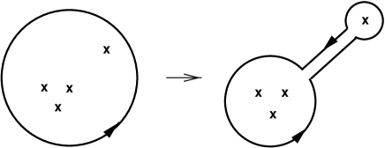
Figure 1: The modification of the contour upon decoupling of one fermion (e.g. from $N_{f}=2$ to $N_{f}=1$). $\times$ represents a singularity in the $u$-plane.

From the above mentioned periodicity of $\theta_{eff}$ in the massive theories it follows that for generic values of $u$ and $m_{i}$, where the only light particles are the photon and its $N=2$ superpartners, the low energy effective theory is CP invariant if $\theta_{eff}$ is an integer multiple of $(4-N_{f})\pi/2$.

4. Global Quark Numbers of Monopoles and Dyons

Another nontrivial manifestation of the lack of CP invariance is the fractionalization of the quark numbers of the solitons. The exact mass formula Eq.(1.6) of Seiberg and Witten for BPS saturated states contains the ${i}$-th quark number $S_{i}$ of the given $(n_{m},n_{e})$ dyon. The knowledge of these quantum numbers is also needed to write down the low energy effective Lagrangian involving light monopoles, near the singularities of QMS. First note however that the low energy effective action (see Eq.(5.1), Eq.(5.5) and Eq.(6.1) below) and the exact mass formula Eq.(1.6) are all invariant under the simultaneous shift

$$a_{D} \to a_{D}+\sum_{i=1}^{N_{f}}c_{i}{m_{i}\over\sqrt{2}};$$

$$S_{i}^{(n_{m},n_{e})} \to S_{i}^{(n_{m},n_{e})}-c_{i}n_{m},$$ (4.1)

where $c_{i}$’s are arbitrary real numbers. At first sight such an invariance might appear to prevent us from determining unambiguously either $S_{i}^{(n_{m},n_{e})}$ or $a_{D}$. For the latter such an ambiguity would appear as an indeterminancy of the integration constant when the exact solution Eq.(1.8) is integrated in $u$. Note that the use of the exact mass formula fixes only the sum of such constants proportional to $m_{i}$’s appearing in Eq.(1.6).

This invariance reflects the fact that, even though the quark number associated to the $i$-th quark (see Table 1) is a good symmetry (conserved and not spontaneously broken), there is no way within the theory to measure it. This is to be contrasted with the case of the electric charge of dyons discussed in the previous section. Of course, one could make the $i$-th quark number observable by gauging weakly the $U_{i}(1)$ symmetry but unless this is done any choice of $S_{i}$’s is as good as another.

Thus within the present theory one can fix $S_{i}$’s by some convention and accordingly determine the integration constants appearing in $a_{D}$. (As was pointed out in [17], the arbitrariness of such a convention should not be confused with the ambiguity of the contour defining $a_{D}$, as to whether or not to pick up certain pole residues. The latter gives rise to the redefinitions of $a_{D}$ by integer multiples of $m_{i}/\sqrt{2}$ only [2], hence could at best be regarded as a particular case of the mentioned arbitrariness of $S_{i}$. Once $a_{D}(u)$ is defined by fixing the contour and the integration constant, those residue contributions are however essential to give the correct monodromy transformations, when $u$ is looped around a singularity [2]. )

For definiteness we take $S_{i}$’s to be the physical $i$-th quark number of a given $(n_{m},n_{e})$ dyon, in the CP invariant theory - the case in which $m_{i}$ and $u$ are all real and in the semiclassical region. This makes sense since the dependences on $m_{i}$’s are explicitly given in the exact solution of Seiberg-Witten (it appears in the form of the curves Eq.(1.7) and in the term proportional to $S_{i}$’s). As is well known, the quark numbers of the magnetic monopoles are half integers in a CP invariant theory[19], see Table 2 and Appendix A.

Our $S_{i}$ can be thought as a possible choice for what was called $s_{i}$ in [17], although the meaning of the latter was somewhat obscure there.

Table 2: Quark numbers of the light dyons in the CP invariant theory; $\pm$ denotes the $SO(2N_{f})$ chirality of the spinor representation. $\theta_{eff}$ gives the value of the effective $\theta$ parameter where the corresponding dyon becomes massless.

$N_{f}=1$

name	S	$n_{m}$	$n_{e}$	$SO(2)$	$\theta_{eff}$
$M$	$-1/2$	1	0	$+$	$0$
$M^{\prime}$	$1/2$	1	1	$-$	$-\pi$
$M^{\prime\prime}$	$-1/2$	1	2	$+$	$-2\pi$

$N_{f}=2$

name	$S_{1}$	$S_{2}$	$n_{m}$	$n_{e}$	$SO(4)$	$SU(2)\times SU(2)$	$\theta_{eff}$
$M_{1}$	$-1/2$	$-1/2$	1	0	$+$	(${\bf 2},\,\,{\bf 1}$)	$0$
$M_{2}$	$1/2$	$1/2$	1	0	$+$	(${\bf 2},\,\,{\bf 1}$)	$0$
$M^{\prime}_{1}$	$1/2$	$-1/2$	1	1	$-$	(${\bf 1},\,\,{\bf 2}$)	$-\pi$
$M^{\prime}_{2}$	$-1/2$	$1/2$	1	1	$-$	(${\bf 1},\,\,{\bf 2}$)	$-\pi$

$N_{f}=3$

name	$S_{1}$	$S_{2}$	$S_{3}$	$n_{m}$	$n_{e}$	$SO(6)$	$SU(4)$	$\theta_{eff}$
$M_{0}$	$-1/2$	$-1/2$	$-1/2$	1	0	$+$	${\bf 4}$	$0$
$M_{1}$	$-1/2$	$1/2$	$1/2$	1	0	$+$	${\bf 4}$	$0$
$M_{2}$	$1/2$	$-1/2$	$1/2$	1	0	$+$	${\bf 4}$	$0$
$M_{3}$	$1/2$	$1/2$	$-1/2$	1	0	$+$	${\bf 4}$	$0$
$M^{\prime}_{0}$	$1/2$	$1/2$	$1/2$	1	1	$-$	${\bf 4^{*}}$	$-\pi$
$M^{\prime}_{1}$	$1/2$	$-1/2$	$-1/2$	1	1	$-$	${\bf 4^{*}}$	$-\pi$
$M^{\prime}_{2}$	$-1/2$	$1/2$	$-1/2$	1	1	$-$	${\bf 4^{*}}$	$-\pi$
$M^{\prime}_{3}$	$-1/2$	$-1/2$	$1/2$	1	1	$-$	${\bf 4^{*}}$	$-\pi$
$N$	$0$	$0$	$0$	2	1		${\bf 1}$	$-\pi/2$

Once the quark numbers $S_{i}$ of dyons are fixed, the integration constant in $a_{D}$ is uniquely determined after specifying the integration contour appropriately. To determine it actually, one can for instance start in a semiclassical region ($u\gg\Lambda^{2}$, $m_{i}\gg\Lambda$), and takes the integration contour (the $\alpha$ cycle) for instance as in Appendix C. The mass of a reference particle (say a $(1,0)$ monopole) should then be computed with the exact mass formula Eq.(1.6) and we determine the integration constant in $a_{D}$ such that it coincides with the standard semiclassical mass formula (see below, Eq.(4.6)) in the appropriate limit. Alternatively, but equivalently, one can work directly in the strong coupling region and require that at the relevant singularity the reference particle becomes massless, according to the mass formula Eq.(1.6). For instance, the $(1,0)$ monopole should be massless at a singularity where the $\alpha$ cycle collapses to a point.

Either way, we arrive at the formula

$$a_{D}(u)=-{\sqrt{2}\over 4\pi}\oint_{\alpha}{dx\,y\over x^{2}}+\sum_{i=1}^{N_{f}}{m_{i}\over 2\sqrt{2}},$$ (4.2)

where the $\alpha$ cycle is such that it reduces to a zero cycle at one of the $(1,0)$ singularities (corresponding to the massless monopole $M$ for $N_{f}=1$, to $M_{1}$ for $N_{f}=2$, and to $M_{0}$ for $N_{f}=3$, in Table 2).

As an example of a possible redefinition of the type, Eq.(4.1), one could choose the classical quark numbers $S_{i}=S_{i}^{(cl)}$ (see Eq.(A.7)) instead of those given in Table 2. In such a convention, $a_{D}$ would be given by the same contour integral as in Eq.(4.2) but without the constant term proportional to $m_{i}$.

Note that, in contrast to the case of $a_{D}$, $a$ does not suffer from the arbitariness, Eq.(4.1); accordingly the integration constant in the case of $a(u)$ can be fixed uniquely by the boundary condition, $a(u)\sim\sqrt{2u}/2$ in the semiclassical region. Alternatively, the integration constant for $a(u)$ may be fixed by the requirement that when a quark mass $m_{i}$ is large there must be a $(0,1)$ singularity at $a=\pm m_{i}/\sqrt{2}$. For $N_{f}=1$, for instance, this gives the expression

$$a(u)=-{\sqrt{2}\over 4\pi}\oint_{\beta}{dx\,y\over x^{2}}+{m\over\sqrt{2}},$$ (4.3)

where the cycle $\beta$ is chosen so as to encircle the two smaller branch points. See Appendix C for further discussions.

Of course, in a CP noninvariant theory the physical $U_{i}(1)$ charges of the dyons differ from those given in the Table 2: they are in general fractional, not even half integers. In the semiclassical limit they can be computed in the standard manner; in the present context, Ferrari has obtained [17]:

$$S_{i}^{(phys)}\simeq S_{i}^{(cl)}+{n_{m}\over 2\pi}\hbox{\rm Arg}{a+m_{i}\,/\sqrt{2}\over m_{i}/\sqrt{2}-a},$$ (4.4)

where $S_{i}^{(cl)}$ denotes the integer classical (or canonical) $i$-th quark number, Eq.(A.7). For the semiclassical dyons the classical charges are simply the excitation numbers of fermion zero modes (see Appendix A). The mass of a dyon is given semiclassically by $\sqrt{2}|Z_{cl}|$ where

$$Z_{cl}\simeq a\left({2\over g}Q_{e}+i{8\pi\over g^{2}}n_{m}\right)+{1\over\sqrt{2}}\sum_{i=1}^{N_{f}}\,m_{i}S_{i}^{(phys)}.$$ (4.5)

By using Eq.(3.12) and Eq.(4.4), this can be rewritten as

$$Z_{cl} \simeq an_{e}+(-{4\over\pi}\hbox{\rm Arg}\,a+i{8\pi\over g^{2}})a\,n_{m}+{n_{m}\over 2\pi}\sum_{i=1}^{N_{f}}\,\left[(a-{1\over\sqrt{2}}m_{i})\,\hbox{\rm Arg}\,({m_{i}\over\sqrt{2}}-a)+\right.$$ (4.6)

$$+\left.(a+{1\over\sqrt{2}}m_{i})\,\hbox{\rm Arg}\,({m_{i}\over\sqrt{2}}+a)\right]+{1\over\sqrt{2}}\sum_{i=1}^{N_{f}}\,m_{i}S_{i}^{(cl)}.$$

Again, such a result must be consistent with the exact Seiberg Witten solution in the appropriate, semiclassical limit. The latter gives, as is seen easily upon integration of Eq.(3.14) with respect to $a$,

$$a_{D}\!\! \simeq \!\!{i\over\pi}\left\{4a\log a-{1\over 2}\sum_{i=1}^{N_{f}}\,[\,(a-{m_{i}\over\sqrt{2}})\log(a-{m_{i}\over\sqrt{2}})+(a+{m_{i}\over\sqrt{2}})\log(a+{m_{i}\over\sqrt{2}})\,]+\right.$$ (4.7)

$$\left.+[\,(8-{N_{f}\over 2})\log 2-(4-N_{f})\,]a-i{N_{f}\pi\over 2}a\right\}+\sum_{i=1}^{N_{f}}{m_{i}\over 2\sqrt{2}}.$$

Inserted in the exact mass formula, Eq.(1.6), this is seen to reproduce precisely the electric and quark number charge fractionalization effects in the semiclassical formula Eq.(4.6), besides the one-loop renormalization corrections (which were not included in the latter). This confirms the claim in Ref. [17] that the quark number fractionalization effects reside in $a_{D}$, but the main point of our result is that it provides a new, far-from-trivial check of the correctness of the Seiberg Witten solution, Eq.(1.7) and Eq.(1.8).

As a by-product of this analysis, the above semiclassical mass formula can be used to study how the spectrum of various dyons depends on the vacuum parameter. For simplicity we consider the case $m_{i}=0,$ $\forall i$. Indeed, in such a case the $\theta$ dependence appears in the semiclassical formula only through the factor, $|2aQ_{e}/g_{eff}|^{2}=|n_{e}+(\theta_{eff}/\pi)n_{m}|^{2}$, with $\theta_{eff}\simeq\theta_{0}-{\pi\over 2}N_{f}$. The value of $\theta_{eff}$ parameter where a given semiclassical dyon takes a local minimum, is shown in the last column of Table 2. We note that the “lightest dyon” is always electrically neutral (monopole), and furthermore the values of $\theta_{eff}$ in Table 2 is in agreement with those at the singularities, Eq.(3.10); it is natural to conjecture that these lightest semiclassical dyons are smoothly connected along a straight path at fixed ${\hbox{\rm Arg }}\,u$, to the massless dyon at the singularity lying on the same ray.

5. $N=1$ Perturbation and Low Energy Monopole Effective Action

We are now in a position to write down and discuss the low energy effective Lagrangian near the singularities of QMS. To select out these vacua we perturb the theory with a small adjoint mass term, Eq.(1.4). Furthermore, we shall limit our discussion to the cases of small bare quark masses $m_{i}$; if one of them is large, the associated singularity describes a weakly coupled QED like theory of the quark (electron) [2], whose properties are quite standard.

Let us consider the cases $N_{f}=1$ and $N_{f}=2$ in this section, postponing the discussion of the $N_{f}=3$ to the next subsection.

5.1. Effective Lagrangian for $N_{f}=1$

When the bare quark mass $m$ is small, the singularities are near one of the points [2] $u_{1,3}=\exp(\pm i\pi/3)$ and $u_{2}=-1$ (we use the unit $3\cdot 2^{-8/3}\Lambda_{1}^{2}=1$). Let us consider the theory near $u_{3}=\exp(-i\pi/3)$ where a $(1,0)$ monopole $M$ is light. The effective Lagrangian has the form,

$${\cal L} = {1\over 8\pi}Im\,[\int d^{4}\theta\,{(\partial F(A_{D})/\partial A_{D})}{\bar{A}_{D}}+\int d^{2}\theta\,{(\partial^{2}F(A_{D})/\partial A_{D}^{2})}W_{D}W_{D}/2\,]$$ (5.1)

$$+\int d^{4}\theta\,[M^{\dagger}e^{V_{D}}M+{\tilde{M}}^{\dagger}e^{-V_{D}}{\tilde{M}}]+\int d^{2}\theta\,{\cal P}+h.c.,$$

where the superpotential is given by ($S=-1/2$)

$${\cal P}=(\sqrt{2}A_{D}+S\,m){\tilde{M}}M+m_{A}U(A_{D})$$ (5.2)

and $A_{D}(u)$ ($U(A_{D})$ is its inverse) is provided by the Seiberg-Witten solution. By minimizing the superpotential one finds

$$(\sqrt{2}A_{D}-{1\over 2}m)M=0,\quad\sqrt{2}{\tilde{M}}M+m_{A}U^{{}^{\prime}}(A_{D})=0,$$ (5.3)

from which one gets the vacuum expectation values of these fields:

$$\langle M\rangle=\langle{\tilde{M}}\rangle=\left(-{m_{A}U^{{}^{\prime}}(A_{D})\over\sqrt{2}}\right)^{1/2},\quad a_{D}={m\over 2\sqrt{2}}.$$ (5.4)

This shows that the continuous vacuum degeneracy of the $N=2$ theory is indeed lifted and (locally) gives the unique vacuum at $u_{3}=\exp(-i\pi/3)$. As in [1] the magnetic monopole condensation means confinement [24], as expected for a theory which become strongly coupled in the low energies.

Anologous situation presents itself if one starts with the effective Lagrangian near $u_{1}$ or $u_{2}$: each singularity of the $N=2$ QMS leads to an $N=1$ vacuum.

5.2. Effective Lagrangian for $N_{f}=2$

The case of ${N_{f}=2}$ is more interesting because of the presence of a nontrivial chiral symmetry $SO(2N_{f})=SO(4)$ (approximate if $m_{i}\ll\Lambda_{2}$.) There are now four singularities of the QMS of the $N=2$ theory which become the vacua of the $N=1$ theory, by a by-now well understood mechanism through the modification of the superpotential produced by the adjoint mass term. Let us consider the theory near two of the singularities $u_{1,2}$, Eq.(2.2), where two $(1,0)$ dyons $M_{1}$, $M_{2}$ (see Table 2) are light. The effective Lagrangian describes those particles interacting with the dual gauge multiplet $(A_{D},W_{D})$:

$${\cal L} = {1\over 8\pi}Im\,[\int d^{4}\theta\,{(\partial F(A_{D})/\partial A_{D})}{\bar{A}_{D}}+\int d^{2}\theta\,{(\partial^{2}F(A_{D})/\partial A_{D}^{2})}W_{D}W_{D}/2\,]$$ (5.5)

$$+\int d^{4}\theta\,\sum_{i=1}^{2}[M_{i}^{\dagger}e^{V_{D}}M_{i}+{\tilde{M}}_{i}^{\dagger}e^{-V_{D}}{\tilde{M}}_{i}]+\int d^{2}\theta\,{\cal P}+h.c.,$$

where the superpotential is given by (for $S_{i}$ see Table 2)

$${\cal P}=\sum_{i=1}^{2}(\sqrt{2}A_{D}+\sum_{\ell=1}^{2}S_{i}^{\ell}\,m_{\ell}){\tilde{M}}_{i}M_{i}+m_{A}U(A_{D}).$$ (5.6)

Supersymmetric vacua occur where the superpotential is stationary:

$$(\sqrt{2}A_{D}-{m_{1}+m_{2}\over 2})M_{1}=0,\quad M_{1}={\tilde{M}}_{1},$$

$$(\sqrt{2}A_{D}+{m_{1}+m_{2}\over 2})M_{2}=0,\quad M_{2}={\tilde{M}}_{2},$$

$$\sqrt{2}\sum_{i=1}^{2}{\tilde{M}}_{i}M_{i}+m_{A}U^{{}^{\prime}}(A_{D})=0.$$ (5.7)

These equations have two solutions,

$$a_{D}=\langle A_{D}\rangle={m_{1}+m_{2}\over 2\sqrt{2}},\quad M_{2}=0,\quad\langle M_{1}\rangle=\left(-{m_{A}U^{{}^{\prime}}(A_{D})\over\sqrt{2}}\right)^{1/2},$$ (5.8)

and

$$a_{D}=-{m_{1}+m_{2}\over 2\sqrt{2}},\quad M_{1}=0,\quad\langle M_{2}\rangle=\left(-{m_{A}U^{{}^{\prime}}(A_{D})\over\sqrt{2}}\right)^{1/2},$$ (5.9)

corresponding respectively to the $u_{1}$ and $u_{2}$ singularities of the $N=2$ theory. Note in particular the change of the value $\langle A_{D}\rangle$ by $(m_{1}+m_{2})/\sqrt{2}$ in going from $u_{1}$ to the nearby singularity $u_{2}$, found here from the minimization of the effective low energy potential, is consistent with the behavior of the exact solution $a_{D}(u)$. In fact, the two branch points $x_{1}$ and $x_{2}$ coincide both at $u=u_{1}$ and at $u=u_{2}$; however, in the continuation the $\alpha$ cycle defining $a_{D}(u)$ picks up twice the contribution of the residue at $x=-\Lambda_{2}^{2}/8$, which is precisely $(m_{1}+m_{2})/\sqrt{2}$ as explained in [2].

Condensation of the monopole $M_{1}$ or $M_{2}$ leads to confinement (à la ’tHooft-Mandelstam) of the original color charges. But now the monopoles $(M_{1},M_{2})$ form a doublet (2, 1) with respect to the chiral $SU(2)\times SU(2)\sim{\widehat{SO(4)}}$. The latter is therefore spontaneously broken to the group $SU(2)\times U(1).$ Moreover, this chiral symmetry breaking is a consequence of the same mechanism (monopole condensation) that is responsible for confinement.

We note also that in the $m_{i}\to 0$ limit (but with $m_{A}\neq 0$), the monopoles $M_{2},\,{\tilde{M}}_{2}$ (four real scalars) remain strictly massless. They describe the three Nambu-Goldstone bosons of the chiral symmetry breaking $SU(2)\times SU(2)\to SU(2)\times U(1)$ and two superpartners. All other scalars contained in $A_{D},\,\,M_{1}$ and ${\tilde{M}}_{1}$ become massive. (Their masses can be analysed as in [15].)

In the strictly massless case ($m_{1}=m_{2}=0$) the symmetry breaking pattern is slightly different. Actually, the problem of finding the minima of the potential in this case reduces to that of finding the classical vacua in the SQED with two flavors, discussed in Sec. 2.5 of [2]. The vacua has the general form (up to symmetry transformations), $M=(C,0);\,\,{\tilde{M}}=-{\mu/\sqrt{2}C},B),$ where $\mu=m_{A}U^{{}^{\prime}}(0)$, and $B$ and $C$ are arbitrary complex numbers satisfying $|C|^{2}=|B|^{2}+|C|^{2}/2|C|^{2}.$ The global symmetry is now broken as $SU(2)\times SU(2)\to SU(2).$

Though the pattern of the chiral symmetry breaking is at first sight similar to what is believed to occur in the two-flavored QCD, the details are different, because of the peculiar interactions special to the $N=2$ supersymmetry. In particular the second $SU(2)$ factor in the $SU(2)\times SU(2)\sim{\widehat{SO(4)}}$ symmetry is not analogous to the axial $SU_{A}(2)$ in QCD (the other $SU(2)$ is the standard vector $SU_{V}(2)$.) The properties of Nambu-Goldstone bosons (singlets of the remaining $SU(2)$) are also quite different from the case of QCD.

The theories near the other two singularities $u_{3,4}$ where the $(1,1)$ ”dyon” $M^{\prime}_{1,2}$ are light, can be analysed in a similar manner. As explained in Sec 3.2., the $(1,1)$ particles are actually pure magnetic monopoles with zero electric charge.

6. Oblique Confinement at $N_{f}=3$

The three ($N_{f}=1$) or the two pairs of singularities ($N_{f}=2$) studied above are physically quite similar when all bare quark masses are small: in fact, in the limit of zero bare masses they are related by exact symmetries, $Z_{3}$ (for $N_{f}=1$) or $Z_{2}$ (for $N_{f}=2$).

In contrast, the singularity near $u^{{}^{\prime}}={\Lambda_{3}^{2}/256}$ at which the $(2,1)$ dyon becomes light, and the quartet of nearby singularities around $u^{{}^{\prime}}=0$ associated with four $(1,0)$ monopoles, which occur in the $N_{f}=3$ case, are physically very distinguished. Indeed, while the quartet of singularities are associated with $(1,0)$ monopoles carrying flavor quantum number 4 of $SU(4)={\widehat{SO(6)}}$ (see also the $S_{i}$ quantum numbers of $M_{i}$’s in Table 2.), the singularity near $u^{{}^{\prime}}={\Lambda_{3}^{2}/256}$ is due to a $(2,1)$ dyon which is flavor neutral.

The analysis of the low energy effective Lagrangians is similar to the cases of $N_{f}=1$ or $N_{f}=2$. Near the quartet singularities, one has

$${\cal L} = {1\over 8\pi}Im\,[\int d^{4}\theta\,{(\partial F(A_{D})/\partial A_{D})}{\bar{A}_{D}}+\int d^{2}\theta\,{(\partial^{2}F(A_{D})/\partial A_{D}^{2})}W_{D}W_{D}/2\,]$$ (6.1)

$$+\int d^{4}\theta\,\sum_{i=0}^{3}[M_{i}^{\dagger}e^{V_{D}}M_{i}+{\tilde{M}}_{i}^{\dagger}e^{-V_{D}}{\tilde{M}}_{i}]+\int d^{2}\theta\,{\cal P}+h.c.,$$

where the superpotential is given by ($S_{i}$ in Table 2)

$${\cal P}=\sum_{i=0}^{3}(\sqrt{2}A_{D}+\sum_{\ell=1}^{3}S_{\ell}^{i}\,m_{\ell}){\tilde{M}}_{i}M_{i}+m_{A}U(A_{D}),$$ (6.2)

Minimization of the scalar potential leads to one of the four vacua:

$$a_{D}=\langle A_{D}\rangle={m_{1}+m_{2}+m_{3}\over 2\sqrt{2}},\quad M_{i}=0,\,(i\neq 0),\quad\langle M_{0}\rangle=(-{m_{A}U^{{}^{\prime}}(A_{D})\over\sqrt{2}})^{1/2},$$

$$a_{D}={-m_{1}-m_{2}+m_{3}\over 2\sqrt{2}},\quad M_{i}=0,\,(i\neq 1),\quad\langle M_{1}\rangle=(-{m_{A}U^{{}^{\prime}}(A_{D})\over\sqrt{2}})^{1/2},$$

$$a_{D}={-m_{1}+m_{2}-m_{3}\over 2\sqrt{2}},\quad M_{i}=0,\,(i\neq 2),\quad\langle M_{2}\rangle=(-{m_{A}U^{{}^{\prime}}(A_{D})\over\sqrt{2}})^{1/2},$$

$$a_{D}={m_{1}-m_{2}-m_{3}\over 2\sqrt{2}},\quad M_{i}=0,\,(i\neq 3),\quad\langle M_{3}\rangle=(-{m_{A}U^{{}^{\prime}}(A_{D})\over\sqrt{2}})^{1/2}.$$ (6.3)

In any one of them monopole condensation leads to color confinement and at the same time, to dymanical chiral symmetry breaking, $SO(6)\to SU(3)\times U(1)$. In the limit of zero bare quark masses three of $(M_{i},{\tilde{M}}_{i})$ pairs remain massless ($12$ massless scalars); $6$ of them are the Nambu-Goldstone bosons.

Again, in the case of strictly zero bare masses (not the limit of massive theory) some nontrivial vacuum degeneracy remains, and in a generic such vacuum, the symmetry is broken as $SO(6)\to SU(2)\times U(1)$.

All this has some similarity to what happens in the three-flavored QCD at low energies, though the details are different (for instance, the massless particles here are in the 3 of the remaining $SU(3)$ symmetry, while the pions in QCD are octets).

On the other hand, near the $(2,1)$ singularity, we have the low energy theory

$${\cal L} = {1\over 8\pi}Im\,[\int d^{4}\theta\,{(\partial F(A_{D})/\partial A_{D})}{\bar{A}_{D}}+\int d^{2}\theta\,{(\partial^{2}F(A_{D})/\partial A_{D}^{2})}W_{D}W_{D}/2\,]$$ (6.4)

$$+\int d^{4}\theta\,[N^{\dagger}e^{V_{D}^{{}^{\prime}}}N+{\tilde{N}}^{\dagger}e^{-V_{D}^{{}^{\prime}}}{\tilde{N}}]+\int d^{2}\theta\,{\cal P}+h.c.,$$

where $A_{D}^{{}^{\prime}}\equiv 2A_{D}+A$, $V_{D}^{{}^{\prime}}\equiv 2V_{D}+V$ and the superpotential is given by

$${\cal P}=\sqrt{2}A_{D}^{{}^{\prime}}{\tilde{N}}N+m_{A}U(A_{D}^{{}^{\prime}}).$$ (6.5)

Minimization of the scalar potential in this case leads to the condensation of the $(2,1)$ magnetic monopole (confinement); however no chiral symmetry breaking occurs in this vacuum, $N$ being flavor neutral.

This can be seen as an explicit realization of the oblique confinement of ’t Hooft. The dyons in this theory appear in a spinor representation of the flavor group, $SO(6)\sim SU(4)$. In fact, the quartet $M_{i}$ in 4 of $SU(4)$ (Table 2) can be naturally identified, if transported smoothly in QMS into the semiclassical domain, with the states

$$|M_{0}\rangle;\quad|M_{1}\rangle=b_{2}^{\dagger}b_{3}^{\dagger}|M_{0}\rangle;\quad|M_{2}\rangle=b_{3}^{\dagger}b_{1}^{\dagger}|M_{0}\rangle;\quad|M_{3}\rangle=b_{1}^{\dagger}b_{2}^{\dagger}|M_{0}\rangle,$$ (6.6)

where $|M_{0}\rangle$ is the ”ground state of the monopole sector”, $b_{i}|M_{0}\rangle=0$. See Appendix A.

On the other hand, $N$ can be naturally interpreted as the bound state of the above $M_{i}$ states (4 of $SU(4)$) and the $(1,1)$ states $M^{{}^{\prime}}$ which belong to 4^∗ of $SU(4)$, constructed as

$$|M^{{}^{\prime}}_{0}\rangle=b_{1}^{\dagger}b_{2}^{\dagger}b_{3}^{\dagger}|M_{0}\rangle;\quad|M_{1}^{{}^{\prime}}\rangle=b_{1}^{\dagger}|M_{0}\rangle;\quad|M_{2}^{{}^{\prime}}\rangle=b_{2}^{\dagger}|M_{0}\rangle;\quad|M_{3}^{{}^{\prime}}\rangle=b_{3}^{\dagger}|M_{0}\rangle.$$ (6.7)

Their quark numbers $(S_{1},S_{2},S_{3})$ are given in Table 2, as is readily verified by using the formula, Eq.(A.6). Note that the electric charges of the $M_{i}$ and $M_{i}^{{}^{\prime}}$ dyons in the vacuum near $u^{{}^{\prime}}=\Lambda_{3}^{2}/256$ (where $\theta_{eff}=-\pi/2$, see Eq.(3.8)) are

$${(2/g_{eff})}Q_{e}(M_{i})=-{1\over 2},\qquad{(2/g_{eff})}Q_{e}(M_{i}^{{}^{\prime}})={1\over 2};$$ (6.8)

we conjecture that their strong electrostatic attractions make their bound state much lighter than each of them. That would be precisely the phenomenon conjectured by t’Hooft [24] for QCD at $\theta=\pi$.

The existence of a classical solution corresponding to the $N$ state, conjectured by Seiberg and Witten[2] and later found in [25], does not contradict such an interpretation, since in the limit of large separations such a state is equivalent to the two-particle state made of $M_{i}$ and $M_{i}^{{}^{\prime}}$.

One might wonder why oblique confinement occurs in the $N_{f}=3$ model, while not for $N_{f}=1$ or $N_{f}=2$. Could not the singularity structure of the QMS in this case such that in one group of vacua (for small $m_{i}$) $M_{i}$’s are light, and in the other $M_{i}^{*}$ are, such that in each vacuum there is ordinary confinement? What is the criterion for ordinary or oblique confinement to be realized?

We have no general answer to these questions, though some remarks can be made. To realize the above mentioned alternative dynamical possibility, the theory with $N_{f}=3$ would need eight vacua at the ultraviolet cutoff, since the number of linearly independent states annihilated by supersymmetry generators is expected to remain invariant when the scale is varied from the ultraviolet to infrared. The bare theory in this case however possesses only $N_{f}+2=5$ vacua as was seen in Sec 2.; such scenario is not allowed dynamically. The scenario realized in the exact Seiberg-Witten solution - oblique confinement at $u^{{}^{\prime}}\simeq{\Lambda_{3}^{2}/256}$ and ordinary confinement near $u^{{}^{\prime}}\simeq 0$ (four vacua) - precisely matches with the five vacua present in the ultraviolet theory. Unfortunately, this explanation hinges crucially on the specific properties of supersymmetric theories, not easily generalizable to ordinary theories.

7. Soft Supersymmetry Breaking and $\theta$ Parameter Dependence of Vacuum Energy Density

As a further check that physics discussed so far is reasonable, we study in this section the response of the system to a small perturbation which breaks supersymmetry. The analysis is a straightforward generalization of that made in [16] (see also [26]) in the case of $N_{f}=0$, hence will be discussed only briefly. We start with the $N=1$ theory with small adjoint mass $m_{A}$, Eq.(1.4), and for simplicity we set all bare quark masses to zero in this section.

As a simple model of soft supersymmetry breaking we consider adding

$$\Delta^{{}^{\prime}}L=m^{{}^{\prime}2}\hbox{\rm Tr}\Phi^{2}|_{0}+h.c.$$ (7.1)

as perturbation. ($|m^{{}^{\prime}}|\ll|m_{A}|\ll|\Lambda|$.) Since this theory has a finite number of well defined, locally isolated vacua, the effect of the supersymmetry breaking term Eq.(7.1) on the energy density can be computed to first order, by using the standard perturbation theory:

$$\Delta E=-\langle\Delta^{{}^{\prime}}L\rangle=-m^{{}^{\prime}2}u+h.c.$$ (7.2)

where $u$ is the unperturbed (i.e. $N=1$) vacuum expectation value which is known for each vacuum. The shift of energy density in general eliminates the residual, $N_{f}+2-$ple vacuum degeneracy. As the bare $\theta$ parameter is varied, however, each of these local minima in turn will play the role of the unique, true vacuum of the theory.

We shall illustrate the situation for $N_{f}=1$. In the three $N=1$ vacua $u$ takes the values

$$u_{1}=e^{\pi i/3}A,\quad u_{2}=-A,\quad u_{3}=e^{-\pi i/3}A,$$ (7.3)

where $A\equiv 3\cdot 2^{-8/3}\Lambda_{1}^{2}$. The phase of $A$ is found by the observation that for general $N_{f}$ ($N_{f}=1,2,3$), $\Lambda_{N_{f}}$ depends on $\theta_{0}$ and on $g$ through the combination,

$$\Lambda_{N_{f}}=\mu\,e^{\pi\tau i/(4-N_{f})},\quad\tau={\theta\over\pi}+{8\pi i\over g^{2}}.$$ (7.4)

For $N_{f}=1$ it means that $A\propto\exp{2i\theta_{0}/3}$. Therefore one finds from Eq.(7.2) the dependence of the energy density in the three local minima on $\theta_{0}$:

$$\Delta E=-2|m^{{}^{\prime}2}A|\,\cos({2\theta_{0}\over 3}+{\pi\over 3}+2\hbox{\rm Arg}m^{{}^{\prime}}),\quad u\simeq u_{1},$$

$$\Delta E=-2|m^{{}^{\prime}2}A|\,\cos({2\theta_{0}\over 3}+{\pi}+2\hbox{\rm Arg}m^{{}^{\prime}}),\quad u\simeq u_{2},$$

$$\Delta E=-2|m^{{}^{\prime}2}A|\,\cos({2\theta_{0}\over 3}-{\pi\over 3}+2\hbox{\rm Arg}m^{{}^{\prime}}),\quad u\simeq u_{3}.$$ (7.5)

These are illustrated in Fig.2 where the vertical scale is arbitrary.

Figure 2: Energy density in the three minima as a function of $\theta_{0}^{{}^{\prime}}$

The true vacuum is thus near $u_{1}$, $u_{3}$ and $u_{2}$, for the value of $\theta_{0}^{{}^{\prime}}\equiv\theta_{0}+3\hbox{\rm Arg}m^{{}^{\prime}}$ which lie in the regions, $-\pi<\theta_{0}^{{}^{\prime}}<0;$ $0<\theta_{0}^{{}^{\prime}}<\pi;$ $\pi<\theta_{0}^{{}^{\prime}}<2\pi,$ respectively. Note that, in spite of the appearance of the cosine of angle ${2\theta_{0}/3}$, the energy density of the true vacuum is a periodic function of $\theta_{0}$ with period $\pi$, in accordance with the general discussion of Sec. 3.1. At $\theta_{0}^{{}^{\prime}}=n\pi,$ $n=$ an integer, the vacuum is doubly degenerate, CP is spontaneously broken à la Dashen [27]. As long as $m^{{}^{\prime}}$ is small, the vev $u$ remains near one of the $N=2$ singularities (at $\theta_{0}^{{}^{\prime}}=n\pi$ it jumps from one local minimum to another), meaning that $\theta_{eff}\ll 1,$ independently of the value of $\theta_{0}:$ CP is only slightly broken. The $M$ particle which condenses is a true dyon with small nonzero electric charge.[16] Confinement persists at nonzero $\theta_{0}$, in contrast to the conjecture of [28] but in accord with [29].

The analysis can be repeated for $N_{f}=2$ or $N_{f}=3$: in all massless cases, the periodicity in $\theta_{0}$ of the energy density of the vacuum is found to be $\pi$ reflecting the $Z_{4-N_{f}}$ symmetry in the $N=2$ theories. The phase diagram in the cases $N_{f}=1$ and $N_{f}=3$ are shown in Fig.3. In the massive cases, the discrete symmetry $Z_{4-N_{f}}$ is explicitly broken: the periodicity in $\theta_{0}$ is reduced to $(4-N_{f})\pi$.

Figure 3: The $\theta^{\prime}_{0}$ dependence of the phase structure in the cases $N_{f}=1$ and $N_{f}=3$.

8. Vacuum Structure of the $N=1$ Effective Theories involving ”Meson” Fields

In previous sections we examined the $\theta$ angle dependence of the low energy effective theories involving magnetic monopoles, in the case the adjoint mass $m_{A}$ was small. (In fact, these effective actions are smoothly connected to the $N=2$ actions in the $m_{A}\to 0$ limit.) For large adjoint masses, however, these effective theories are not the proper low-energy descriptions of the theory. The more adequate low energy theory in those cases should involve ”meson” variables $V^{IJ}=-V^{JI}=\hat{Q}^{I}\hat{Q}^{J}$ instead [2, 30, 31], and contain the superpotential $(1/m_{A})(V_{IJ})^{2}$ obtained after the integration of the heavy adjoint fields. In the limit,

$$m_{A}\rightarrow\infty;\quad\tilde{\Lambda}_{N_{f}}^{6-N_{f}}=m_{A}^{2}\Lambda_{N_{f}}^{4-N_{f}}\quad{\hbox{\rm fixed}},$$ (8.1)

these theories must smoothly be connected to the ordinary N=1 $SU(2)$ SQCD with $N_{f}$ flavors.

For intermediate values of $m_{A}$, we have thus two equivalent descriptions of vacua [2]; one involving the meson fields, and the other in terms of the photon and monopole fields. The number of vacua and the $\theta$ dependence following from the low energy description involving meson fields must be the same as those found in Sec.3. On the other hand, these properties should also match those of the N=1 SQCD vacua in the limit, Eq.(8.1).

For example, for $N_{f}=1$ the only independent composite field is $V^{12}=iQ\tilde{Q}=iT$. The exact superpotential [30] is given by

$$W_{N_{f}=1}=\frac{m_{A}^{2}\Lambda_{1}^{3}}{T}-\frac{1}{m_{A}}T^{2}+mT.$$ (8.2)

First consider the massless case ($m=0$). The vev of T is given by the solution of $T^{3}=-m_{A}^{3}\Lambda_{1}^{3}/2$: there are three distinct vacua, just as in the $N_{f}=1,$ $N=2$ theory. In fact, these three vacua are related by the phase rotation of $T=Q\tilde{Q}$ field by $e^{i\pi/3}$ which is equivalent to the shift of $\theta$ by $\pi$, in agreement with the $\pi$ periodicity of the underlying theory.

For nonzero bare quark mass $m$, there are still three vacua, however, they are no longer related by a $Z_{3}$ symmetry in $U(1)_{R}$ transformation. Therefore the periodicity in $\theta$ is reduced to $3\pi$, again in agreement with the discussion of Sec.3.2.

However when the adjoint fields are truly decoupled in the limit, Eq.(8.1), the $U(1)_{A}$ transformation becomes an independent chiral transformation (see Table 1). As a result the periodicity in $\theta$ gets back to $\pi$, which is the correct periondicity of the massive $SU(2)$ SQCD.

In the $N=1$ limit, Eq.(8.1), we indeed recover all the known results of $N=1$ SQCD with a single flavor: all vacua ”run away” ($T\to\infty$) in the $m\to 0$ limit. On the other hand, if $m\neq 0$ there remain two vacua with finite vev $T_{1},T_{2}$ (in accordance with the Witten’s index for a massive $SU(2)$ gauge theory), though the vacuum with $T_{3}$ runs away:

$$T_{1,2}\sim\pm\left({m_{A}^{2}\Lambda_{1}^{3}\over 2m}\right)^{1/2},\qquad T_{3}\sim 2mm_{A}\,\rightarrow\,\infty.$$ (8.3)

Here the running solution is just the “special point” found through the classical analysis done in Sec 2.

A similar check of the number of vacua as well as the $\theta$ angle dependence in the low energy $N=1$ effective theories with meson degrees of freedom, can be made in the cases $N_{f}=2$ and $N_{f}=3$, using the superpotential [30],

$$W_{N_{f}=2} = X(\mbox{Pf}V-m_{A}^{2}\Lambda_{2}^{2})+W_{\mbox{tree}},$$

$$W_{N_{f}=3} = -\frac{\mbox{Pf}V}{m_{A}^{2}\Lambda_{3}}+W_{\mbox{tree}},$$ (8.4)

where

$$W_{\mbox{tree}}=\frac{1}{8m_{A}}\mbox{Tr}V^{2}+\sum_{i=1}^{N_{f}}m_{i}V^{2i-1,2i}.$$ (8.5)

In all cases we find the correct $\theta$ periodicity, which is $\pi$ (zero bare quark masses), or $(4-N_{f})\pi$ (nonzero bare quark masses). Also, in the massless case one finds the continuous vacuum degeneracy, corresponding to the ”Higgs” branch of vacua of the underlying $N=2$ theory. In the massive cases the Higgs branches disappear, instead there remain the $N_{f}+2$ distinct vacua. Again $N_{f}$ of them correspond to the ”special points”, and run away to infinity in the $N=1$ limit.

9. Conclusion

In this paper we explored several dynamical aspects of the $SU(2)$ Seiberg-Witten models with quark hypermultiplets, with a hope to learn more about the detailed behaviors of a strongly interacting non Abelian gauge theories in four dimensions with fermions. Among others, we have clarified the meaning of the number of $N=1$ vacua (number of singularities of QMS of the $N=2$ theories) as well as the CP properties and $\theta$ angle dependence of the theories with and without bare quark masses. We have shown in particular that the electric charge and quark number fractionalization of dyons is correctly incorporated in the Seiberg-Witten solution, providing a new, strong confirmation of their beautiful results.

The structure of $N=1$ low energy effective Lagrangians and the correlation between the phenomenon of confinement and chiral symmetry breaking are also very interesting. Both dynamical possibilities (i.e., confinement either implies or not chiral symmetry breaking) are realized in various $N=1$ vacua in these models. There seems to be a deep and intriguing relation between the low energy phenomena (confinement or oblique confinement; chiral symmetry breaking) and the structure of classical vacua, though such a stringent UV-IR connection can be seen here only thanks to special properties of supersymmetris theories.

There remains the task of applying what has been learned here to a more realistic field theory model of strong interactions: QCD.

Acknowledgments

The authors acknowledge useful discussions with Andrea Capelli and Camillo Imbimbo. One of us (H.T.) thanks the Dipartimento di Fisica dell’Università di Genova as well as the Genova section of INFN for a warm hospitality. He is also grateful for the financial support by the CNR-JSPS exchange program.

Appendix A: Flavor Quantum Numbers of Magnetic Monopoles

In the presence of $N_{f}$ quark hypermultiplets belonging to the fundamental representation of the $SU(2)$ gauge group, the flavor symmetry is enhanced to $SO(2N_{f})$ (not to $O(2N_{f})$ due to anomaly) due to the equivalence of 2 and 2^∗. The quark chiral fields $Q_{a}^{i}$ and $\tilde{Q}_{i}^{a}$ ($i=1,...,N_{f}$), which are in 2 and 2^∗, may be rearranged to form a set of $2N_{f}$ chiral fields in 2 as $Q_{a}^{2i-1}=Q_{a}^{1}$ and $Q_{a}^{2i}=\epsilon_{ab}\tilde{Q}_{i}^{b}$ ($i=1,...,N_{f}$). To see the $SO(2N_{f})$ symmetry of the present model Eq.(1.1), however, we must consider an $SO(2N_{f})$ vector $\hat{Q}_{a}^{I}$ formed by

$$\hat{Q}_{a}^{2i-1}=\frac{1}{\sqrt{2}}(Q_{a}^{2i-1}+Q_{a}^{2i}),\quad\hat{Q}_{a}^{2i}=\frac{1}{i\sqrt{2}}(Q_{a}^{2i-1}-Q_{a}^{2i}),\qquad(i=1,2,\ldots N_{f}).$$ (A.1)

It is well known[19] that each isospinor Dirac fermion $\psi_{D}^{i}(x)$ ($i=1,...,N_{f}$) posesses one charge self-conjugate zero mode $u_{0}(x)$ in the monopole background. In the semiclassical quantization we expand $\psi_{D}^{i}(x)$ accordingly as

$$\psi_{D}^{i}(x)=b^{i}u_{0}(x)+\mbox{(non-zero modes)},$$

$${{}^{\cal C}\psi_{D}^{i}}(x)=b^{i\dagger}u_{0}(x)+\mbox{(non-zero modes)},$$ (A.2)

where the suffix ${\cal C}$ denotes the charge conjugation. The canonical commutation relation requires $\{b^{i},b^{j\dagger}\}=\delta^{ij}$. The $2^{N_{f}}$ monopole states related by the action of these fermion zero-energy-mode operators are all degenerate. These states form a spinor representation of $SO(2N_{f})$ group: the gamma matrices satisfying the $2N_{f}$ dimensional Clifford algebra are given by

$$\gamma^{2i-1}=b^{i}+b^{i\dagger},\quad\gamma^{2i}=(b^{i}-b^{i\dagger})/i,\qquad i=1,2,\ldots N_{f},$$ (A.3)

and in terms of these the generators of the $SO(2N_{f})$ group are given by:

$$\Sigma_{ij}={1\over 4i}[\gamma_{i},\gamma_{j}],\quad i\neq j,$$ (A.4)

where $i,j=1,\ldots,2N_{f}$. Furthermore, the states with even (odd) number excitations belong to a chiral (anti-chiral) spinor representation, since the $SO(2N_{f})$ chirality operator is defined as

$$\gamma^{2N_{f}+1}=(-i)^{N_{f}}\gamma^{1}\gamma^{2}\cdots\gamma^{2N_{f}}=\prod_{i=1}^{N_{f}}(1-2b^{i\dagger}b^{i}).$$ (A.5)

The $i$-th quark number charges of monopoles $S_{i}$ ($i=1,...,N_{f}$), just correspond to the Cartan subalgebra of $SO(2N_{f})$; $\Sigma_{12},\,\Sigma_{34},\,\ldots,\Sigma_{2N_{f}-1,2N_{f}},\,$ since in a CP invariant theory they are given (in the subspace of the degenerate monopoles) by

$$S_{i}=\int d^{3}x\,{1\over 2}({{}^{\cal C}\psi_{D}^{i}}\psi_{D}^{i}-\psi_{D}^{i}{{}^{\cal C}\psi_{D}^{i}})=b^{i\dagger}b^{i}-1/2=\Sigma_{2i-1,2i}.$$ (A.6)

These charges take values $1/2$ or $-1/2$. We can define also the classical (or canonical) quark number charges of monopoles, given by

$$S_{i}^{(cl)}=b^{i\dagger}b^{i},$$ (A.7)

which are integers.

The generators of the spin group can also be easily constructed from the above; for instance for $N_{f}=2$, the two $SU(2)$ generators can be taken as

$$T_{1}^{\pm}=-{i\over 2}(\Sigma_{23}\pm\Sigma_{41}),\quad T_{2}^{\pm}=-{i\over 2}(\Sigma_{31}\pm\Sigma_{42}),\quad T_{3}^{\pm}=-{i\over 2}(\Sigma_{12}\pm\Sigma_{43}).$$ (A.8)

The important point is that the values of the quark numbers $S_{i}$ and other global quantum numbers taken by each member of a monopole multiplet belonging to a particular spinor representation, are uniquely determined, by using these semiclassical constructions. Once such a connection is established, those values can be used for generic monopole states which are not necessarily semiclassical, and can even become massless. The entries of Table 2 have been determined in this manner.

Appendix B: CP Invariance of the $N_{f}=1$ Theory with $m_{A}\neq 0$, $m=0$

In this Appendix we verify the CP invariance of the effective low energy theory for $N_{f}=1,$ $m_{A}\neq 0$ and $m=0$ described by

$${\cal L} = {1\over 8\pi}Im\,[\int d^{4}\theta\,{(\partial F(A_{D})/\partial A_{D})}{\bar{A}_{D}}+\int d^{2}\theta\,{(\partial^{2}F(A_{D})/\partial A_{D}^{2})}W_{D}W_{D}/2\,]$$ (B.1)

$$+\int d^{4}\theta\,[M^{\dagger}e^{V_{D}}M+{\tilde{M}}^{\dagger}e^{-V_{D}}{\tilde{M}}]+\int d^{2}\theta\,{\cal P}+h.c.,$$

$${\cal P}=\sqrt{2}A_{D}{\tilde{M}}M+m_{A}U(A_{D}).$$ (B.2)

Expanding all scalar fields around their vevs, (we consider for definiteness the vacuum $u=u_{3}$),

$$a_{D}=0,\qquad\langle M\rangle=\langle{\tilde{M}}\rangle=\left(-{m_{A}U^{{}^{\prime}}(0)\over\sqrt{2}}\right)^{1/2},$$ (B.3)

one sees that nontrivial phases appear in the fermion mass terms and in the (generalised) Yukawa interactions,

$$L_{Y} = \sqrt{2}[-\langle M^{\dagger}\rangle\lambda_{D}(\psi_{M}-\psi_{\tilde{M}})+\langle M\rangle\psi_{D}(\psi_{\tilde{M}}+\psi_{M})]+{m\over 2}U^{{}^{\prime\prime}}\!(0)\psi_{D}\psi_{D}]$$ (B.4)

$$+\sqrt{2}[-M^{\prime\dagger}\lambda_{D}\psi_{M}+{\tilde{M}}^{\prime\dagger}\lambda_{D}\psi_{\tilde{M}}-(A_{D}\psi_{M}\psi_{\tilde{M}}+\psi_{D}\psi_{\tilde{M}}M^{{}^{\prime}}+\psi_{D}\psi_{M}{\tilde{M}}^{{}^{\prime}})]$$

$$+{m\over 2}(U^{{}^{\prime\prime}}\!(A_{D})-U^{{}^{\prime\prime}}\!(0))\psi_{D}\psi_{D}\,\,+\,\,h.c.$$

where we introduced $M=\langle M\rangle+M^{{}^{\prime}},{\tilde{M}}=\langle{\tilde{M}}\rangle+{\tilde{M}}^{{}^{\prime}}$. To see the phases appearing in $U^{{}^{\prime}}(0)$ and in $U^{{}^{\prime\prime}}(A_{D}),$ one needs the inverse of the Seiberg-Witten solution [2, 5]

$$a_{D}(u)={1\over 6\sqrt{2}}e^{-2\pi i/3}(u^{3}+1)F\left({5\over 6},{5\over 6};2;1+u^{3}\right).$$ (B.5)

To invert this near $u=u_{3}=\exp(-i\pi/3)$ (in this Appendix we use the unit $3\cdot 2^{-8/3}\Lambda_{1}^{2}=1$ used in [5]), first change the variable from $u$ to $w$ by

$$u=u_{3}(1+w),$$ (B.6)

so that

$$u^{3}+1=u_{3}^{3}(w^{3}+3w^{2}+3w)=-(w^{3}+3w^{2}+3w).$$ (B.7)

Since the hypergeometric function is analytic around the origin with real expansion coefficients, this means that $U(A_{D})$ has an expansion of the form

$$U(A_{D})=u_{3}\{1+w(e^{2\pi i/3}A_{D})\},$$ (B.8)

where $w(x)$ is a power series in $x$ with real coefficients.

The phases appearing in Eq.(B.4) can now be made explicit:

$$\langle M\rangle=(-{m_{A}U^{{}^{\prime}}(0)\over\sqrt{2}})^{1/2}=|\langle M\rangle|e^{{i\over 2}\beta+{\pi i\over 6}};\quad\beta\equiv\hbox{\rm Arg}\,m_{A}$$

$$m_{A}U^{{}^{\prime\prime}}(A_{D})=-m_{A}\,w^{{}^{\prime\prime}}(e^{2\pi i/3}A_{D}).$$ (B.9)

At this point it is a matter of direct check to show that the phase rotations by $U(1)_{R}$ and $U(1)_{J}$ (see Table 1)

$$A_{D}\to e^{-2\pi i/3}A_{D},\quad\psi_{D}\to,e^{-{i\over 2}\beta-{\pi i\over,2}}\psi_{D},$$

$$M^{{}^{\prime}}\to e^{{i\over 2}\beta+{\pi i\over,6}}M^{{}^{\prime}},\quad\psi_{M}\to e^{{\pi i\over 3}}\psi_{M};$$

$$\lambda_{D}\to e^{{i\over 2}\beta-{\pi i\over,6}}\lambda_{D}.$$ (B.10)

(the transformations of ${\tilde{M}}^{{}^{\prime}}$ and $\psi_{\tilde{M}}$ are similar to those of $M$ and $\psi_{M}$), eliminate all the phases from the Lagrangian Eq.(B.4): the theory is indeed invariant under CP.

Appendix C: Contour-integral representations for $a_{D}(u)$ and $a(u)$; semiclassical behavior of $\tau$

First consider the integrals

$${da_{D}\over du}\,=\,{\sqrt{2}\over 8\pi}\oint_{\alpha}{dx\over y},\qquad{da\over du}\,=\,{\sqrt{2}\over 8\pi}\oint_{\beta}{dx\over y},$$ (C.1)

where $y$ is given in the form of $y=[(x-x_{1})(x-x_{2})(x-x_{3})]^{1/2}$ and $\alpha$ and $\beta$ cycles encircling two branch points of $y$ are appropriately chosen as will be specified below. Since these integrals can be expressed in terms of the hypergeometric functions

$${da_{D}\over du}=i{\sqrt{2}\over 4}(x_{2}-x_{1})^{1/2}F\left({1\over 2},{1\over 2};1;{x_{2}-x_{3}\over x_{2}-x_{1}}\right),$$

$${da\over du}=i{\sqrt{2}\over 4}(x_{2}-x_{3})^{1/2}F\left({1\over 2},{1\over 2};1;{x_{2}-x_{1}\over x_{2}-x_{3}}\right),$$ (C.2)

(see [32] for related representations of ${da_{D}/du}$, ${da/du}$, $a_{D}$ and $a$ in terms of the hypergeometric functions), the behavior of the effective theta parameter given in Eq.(3.15) follows from the known asymptotic behavior of the hypergeometric functions.

These asymptotics can however be obtained directly by evaluating the contour integrations in Eq.(C.1) in the semiclassical limit; $|u|,|m_{i}^{2}|\gg\Lambda^{2}$. In the semiclassical region the branch points $x_{1},x_{2},x_{3}$ are approximately given by:

$$x_{1,2}\sim{m\pm(m^{2}-u)^{1/2}\over 4u}\,\Lambda_{1}^{3}\quad(N_{f}=1),$$

$$x_{1,2}\sim{m_{1}m_{2}\pm(m_{1}^{2}-u)^{1/2}(m_{2}^{2}-u)^{1/2}\over 8u}\Lambda_{2}^{2}\quad(N_{f}=2),$$

$$x_{1,2}\sim{m_{1}m_{2}m_{3}\pm(m_{1}^{2}-u)^{1/2}(m_{2}^{2}-u)^{1/2}(m_{3}^{2}-u)^{1/2}\over 8u}\Lambda_{3}\quad(N_{f}=3),$$ (C.3)

and $x_{3}\sim u$ for any $N_{f}$. The integration contours can then be taken so that the $\alpha$ cycle encircles $x_{1}$ and $x_{3}$, and the $\beta$ cycle encircles $x_{1}$ and $x_{2}$, both in the counter-clockwise direction.

Note that once these choices are made, by smoothly varying $m_{i}$ and/or $u$ (possibly avoiding the points where all three branch points meet and at which the low energy theory becomes superconformal invariant [33]), ${da_{D}/du}$ and ${da/du}$ are defined uniquely for any values of $u$ and $m_{i}$. More precisely, they are uniquely defined modulo possible $SL(2,Z)$ redefinitions needed, e.g., when a ”quark singularity” (where a $(0,1)$ particle is massless) at large $m_{i}$ turns into a dyon singularity (where a $(n_{m},n_{e})$ particle is massless) at small $m_{i}$, or when one loops around some singularities (monodromy transformations).

In order to actually evaluate the integrals it is convenient to change the variable from $x$ to $\xi=(x-x_{2})/(x_{1}-x_{2})$, and introduce $\xi_{u}=(x_{3}-x_{2})/(x_{1}-x_{2})\sim u/(x_{1}-x_{2})$. Then the integral for $da/du$ can be immediately evaluated in the semiclassical limit as

$${da\over du}\sim 2{\sqrt{2}\over 8\pi}{1\over\sqrt{u}}\int_{0}^{1}d\xi\,{1\over\sqrt{\xi(1-\xi)}}={1\over 2}{1\over\sqrt{2u}}.$$ (C.4)

One finds then

$$a(u)={1\over 2}\sqrt{2u}\,(1+O({1\over u})),$$ (C.5)

where an appropriate integration constant, as in Eq.(4.2), has to be taken into account.

$da_{D}/du$ is also easily evaluated as

$${da_{D}\over du}\sim 2i{\sqrt{2}\over 8\pi}{1\over(x_{1}-x_{2})^{1/2}}\int_{1}^{\xi_{u}}d\xi\,{1\over\sqrt{\xi(\xi-1)(\xi_{u}-\xi)}}\sim i{\sqrt{2}\over 4\pi}{1\over\sqrt{u}}\{\log\xi_{u}+4\log 2\}.$$ (C.6)

After substituting the explicit values of $x_{i}$ given in Eq.(C.3) for $\xi_{u}$ the asymptotic behavior of $\tau$ for $N_{f}=1,2,3$ is found to be:

$$\tau={da_{D}\over da}\simeq{i\over\pi}\left\{4\log a-{1\over 2}\sum_{i=1}^{N_{f}}\log(a^{2}-{m_{i}^{2}\over 2})-{N_{f}\pi\over 2}i+(8-{N_{f}\over 2})\log 2\right\}+O\left({1\over a}\right).$$ (C.7)

The contour-integral representation for $a_{D}(u)$ and $a(u)$ involve appropriate integration constants. For $N_{f}=1$ integration of Eq.(C.1) yields, apart from an integration constant,

$$I_{\alpha,\beta}={\sqrt{2}\over 8\pi}\oint_{\alpha,\beta}dx\,{-2y\over x^{2}},$$

with the same contours as used for $da_{D}/du$ and $da/du.$ The contours are chosen so as to avoid the pole at $x=0$. Note that this made no difference for Eq.(C.1) but here such a specification is important. If we evaluate $I_{\beta}$ in the asymptotic region as in the case of $da/du$, we find that $I_{\beta}\sim\sqrt{2u}/2-m/\sqrt{2}$, which does not quite satisfy the boundary condition, $a(u)\simeq{(1/2)}\sqrt{2u}$. Adding therefore an appropriate integration constant, one gets, for $N_{f}=1$:

$$a(u)=-{\sqrt{2}\over 4\pi}\oint_{\beta}{dx\,y\over x^{2}}+{m\over\sqrt{2}}.$$ (C.8)

(Alternatively the $\beta$ cycle can be taken so as to encircle the pole at $x=0$; in that case the constant term ${m/\sqrt{2}}$ should be dropped.) Note that the formula Eq.(C.8) has a simple interpretation. At the semiclassical singularty where the two smaller branch points meet the $\beta$ cycle defining $a$ shrinks to a point. The additive constant in Eq.(C.8) is there just to ensure that such a singularity occurs at $a=m/\sqrt{2}.$

Similarly, the integration constant in the cases of $N_{f}=2$ and $N_{f}=3$ can be determined from the requirement that the semiclassical singularity ($u_{i}$) corresponding to the $i$-th massless quark (at which the $\beta$ cycle is defined to shrink to zero) occurs at $a=m_{i}/\sqrt{2}.$ Taking the first quark as the reference system one finds, for all $N_{f}$, that

$$a(u)=\oint_{\beta}\lambda_{SW}+{m_{1}\over\sqrt{2}},$$ (C.9)

where

$$\lambda_{SW}=-{\sqrt{2}\over 4\pi}{dx\,y\over x^{2}-\Lambda_{2}^{4}/64}$$ (C.10)

for $N_{f}=2$; $\lambda_{SW}$ for $N_{f}=3$ has been recently given in a simple form by Álvarez-Gaumé, Marino and Zamora[34]:

$$\lambda_{SW}=-{\sqrt{2}\over 16\pi}{dx\over y}(2x-4u-\sum_{n=1}^{4}{y_{n}x_{n}\over x-x_{n}}),$$ (C.11)

where

$$y_{1}=u-m_{1}m_{2}-m_{1}m_{3}+m_{3}m_{2}-x_{1};\quad x_{1}=c(-m_{1}+m_{2}+m_{3}),$$

$$y_{4}=u+m_{1}m_{2}+m_{1}m_{3}+m_{3}m_{2}-x_{4};\quad x_{4}=c(-m_{1}-m_{2}-m_{3}),$$ (C.12)

and $y_{2}=y_{1}(m_{1}\leftrightarrow m_{2})$, $y_{3}=y_{1}(m_{1}\leftrightarrow m_{3})$, and $c\equiv\Lambda_{3}/8$. (Note some minor misprints in Eq.(2.60) and Eq.(2.62) of [34].)

As one moves from the first singularity $u_{1}$ to the second quark singularity, $u_{2}$, the integration over the $\beta$ cycle picks up the residue at a pole, such that $a(u_{2})={m_{2}/\sqrt{2}},$ and so on.

Finally, the integration constant for $a$ has been discussed in Sec.4. One has

$$a_{D}(u)=-{\sqrt{2}\over 4\pi}\oint_{\alpha}{dx\,y\over x^{2}}+\sum_{i=1}^{N_{f}}{m_{i}\over 2\sqrt{2}},$$ (C.13)

where the $\alpha$ cycle is such that at one of the $(1,0)$ singularities it shrinks to zero.

References

• [1] N. Seiberg and E. Witten, Nucl.Phys. B426 (1994) 19.
• [2] N. Seiberg and E. Witten, Nucl. Phys. B431 (1994) 484.
• [3] A. Klemm, W. Lerche, S. Theisen and S. Yankielowicz, Phys. Lett. B344 (1995) 169; P.C. Argyres and A.F. Faraggi, Phys. Rev. Lett. 74 (1995) 3931; A. Hanany and Y. Oz, Nucl. Phys B452 (1995) 283; P. C. Argyres, M. R. Plesser and A. D. Shapere, Phys. Rev. Lett. 75 (1995) 1699.
• [4] A. Bilal, hep-th/9601007; L. Alvarez-Gaumรฉ and S. F. Hassan, CERN-TH/96-371, hep-th/9701069; M. Peskin, SLAC-PUB-7393, hep-th/9702094.
• [5] F. Ferrari and A. Bilal, Nucl. Phys. B469 (1996) 387; A. Bilal and F. Ferrari, Nucl. Phys. B480 (1996) 589.
• [6] T. Harano and M. Sato, Nucl. Phys. B484 (1997) 167.
• [7] E.Witten, Nucl. Phys. B202 (1982) 253.
• [8] D. Amati, K. Konishi, Y. Meurice, G.C. Rossi and G. Veneziano, Phys. Reports, C 162 (1988) 169.
• [9] A. Kovner and M. Shifman, hep-th/9702174, to appear in Phys Rev D56 (1997).
• [10] K. Konishi, Phys. Lett. B135 (1984) 439.
• [11] G. Veneziano and S. Yankielowicz, Phys. Lett. B113 (1982) 321; T. R. Taylor, G. Veneziano and S. Yankielowicz, Nucl. Phys. B218 (1983) 493.
• [12] D. Finnel and P. Pouliot, Nucl. Phys. B453 (1995) 225; N. Dorey, V. V. Khoze and M. Mattis, Phys. Rev. D54 (1996) 2921; ibid 7832; H. Aoyama, T. Harano, M. Sato and S. Wada, Phys. Lett. B388 (1996) 331; F. Fucito and G. Travaglini, Phys.Rev. D55 (1997) 1099-1104; K. Ito and N. Sasakura, Nucl. Phys. B484 (1997) 141.
• [13] T.D. Lee, Physics Reports C 9 (1974) 143.
• [14] K. Ito and S. K. Yang, Phys. Lett. B366 (1996) 165.
• [15] M. Di Pierro and K. Konishi, Phys. Lett. B 388 (1996) 90.
• [16] K. Konishi, Phys. Lett. B392 (1997) 101.
• [17] F. Ferrari, Phys. Rev. Lett. 78 (1997) 795.
• [18] E. Witten, Phys. Lett. B86 (1979) 283.
• [19] R. Jackiw and C. Rebbi, Phys. Rev. D13 (1976) 3398.
• [20] J. Goldstone and F. Wilczek, Phys. Rev. Lett. 47 (1981) 986.
• [21] A.J. Niemi, M.B. Paranjape and G.W. Semenoff, Phys. Rev. Lett 53 (1984) 515.
• [22] S. Coleman, Erice Lectures (1977), ed. A. Zichichi.
• [23] Y. Ohta, J. Math. Phys. 37 (1996) 6074; ibid 38 (1997) 682.
• [24] G. โ€™t Hooft, Nucl. Phys. B190[FS3] (1981) 455; S. Mandelstam, Phys. Rep. 23 (1976) 245.
• [25] J. P. Gauntlett and J. A. Harvey, Nucl. Phys. B 463 (1996) 287.
• [26] N. Evans, S. D. H. Hsu and M. Schwetz, Nucl. Phys. B484 (1997) 124.
• [27] R. F. Dashen, Phys. Rev 183 (1969) 1245; ibid D3 (1971) 1879.
• [28] G. Schierholz, Nucl. Phys. B(Proc. Suppl.) 37A (1994) 203.
• [29] J. L. Cardy and E. Rabinovici, Nucl. Phys. B205[FS5] (1982) 1; J. L. Cardy, Nucl. Phys. B205[FS5] (1982) 17.
• [30] N. Seiberg, Phys. Rev. D50 (1994) 1092; K. Intriligator and N. Seiberg, Nucl. Phys. B431 (1994) 551.
• [31] S. Elitzur, A. Forge, A. Giveon and E. Rabinovici, Phys. Lett. B353 (1995) 79.
• [32] T. Matsuda and H. Suzuki, hep-th/9609066.
• [33] P. C. Argyres and M. R. Douglas, Nucl. Phys. B448 (1995) 93; P. C. Argyres, M. R. Plesser, N. Seiberg and E. Witten, Nucl. Phys. B461 (1996) 71; T. Eguchi, K. Hori, K. Ito and S. K. Yang, Nucl. Phys. B471 (1996) 430; A.Bilal and F. Ferrari, hep-th/9706145.
• [34] L. รlvarez-Gaumรฉ, M. Marino and F. Zamora, hep-th/9703072.