Classical Inhomogeneities in String Cosmology

Abstract

We generalize previous work on inhomogeneous pre-big bang cosmology by including the effect of non-trivial moduli and antisymmetric-tensor/axion fields. The general quasi-homogeneous asymptotic solution—as one approaches the big bang singularity from perturbative initial data—is given and its range of validity is discussed, allowing us to give a general quantitative estimate of the amount of inflation obtained during the perturbative pre-big bang era. The question of determining early-time “attractors” for generic pre-big bang cosmologies is also addressed, and a motivated conjecture is advanced. We also discuss S-duality-related features of the solutions, and speculate on the way an asymptotic T-duality symmetry may act on moduli space as one approaches the big bang.

I Introduction

After some pioneering work [1], string cosmology took a new turn with the realization that, as a result of its duality symmetries [2, 3], it naturally provides, even in the absence of potential energy, standard (FRW) as well as inflationary cosmologies. The crucial role of a dynamical dilaton in providing inflation then became clear.

This observation led to the idea of the so-called pre-big bang (PBB) scenario [4, 5] according to which the Universe started its evolution from a very perturbative initial state, i.e. from very weak coupling and very small curvatures. It then inflated towards larger (space-time) curvatures and coupling during the pre-big bang phase and, possibly after a stringy epoch, eventually made a transition (exit) to the standard radiation-dominated era.

While early work concentrated mostly on homogeneous, Bianchi I-type cosmologies, and on small perturbations around them, a number of extensions of the original scenario have been considered more recently, including some [6] trying to incorporate the latest theoretical developments in string theory. Within a more traditional string theory framework, a more general setting was recently considered [7]. In that approach, given some initial data deeply inside the perturbative region, but otherwise arbitrary, their evolution is followed towards the big bang singularity in the future. It turns out that the evolution of fairly homogeneous initial patches can be described analytically and that a large fraction of those patches inflates, becoming increasingly flat, homogeneous and isotropic. In the special case of exactly homogeneous and isotropic—but non spatially flat—cosmologies, explicit solutions can be found [8] [9]. Also, some scepticism on the naturalness of the PBB picture arose [9].

If the above results are coupled to the assumption that a “graceful exit” does indeed take place (see [10] for recent progress on this issue), the usually assumed Big Bang conditions (a hot, dense and highly-curved state) will be the outcome—rather than the starting point—of inflation. Several interesting phenomenological consequences of the whole scenario have been worked out, particularly on the possibility of generating an interesting spectrum of gravitational waves [11] and of cosmic magnetic fields [12]. Of particular relevance could be the recent observation [13] that pre-big bang cosmology can lead to a scale-invariant spectrum of axionic perturbations.

The purpose of this work is to improve on the results of [7] in various respects, as explained in the following outline: in Sec. II, we formulate the problem directly in the string frame while adding extra dimensions as well as the antisymmetric-tensor field $B_{\mu\nu}$. We thus recover the results of [7] and are able to extend them to the case of quasi-homogeneous $B_{\mu\nu}$, $g_{\mu\nu}$ and $\phi$ fields. In Sec. III we re-express the four-dimensional case with torsion and a single internal-space modulus in terms of the axion field and construct the general asymptotic solution for a quasi-homogeneous axion background. We also look at the solutions in the Einstein frame in order to expose, as simply as possible, their S-duality properties. In Sec. IV we discuss the limits of validity of our asymptotic solutions, from the point of view of both the breakdown of the tree-level low-energy effective action and of that of the gradient expansion. We are thus able to estimate the duration of the PBB era and the number of e-folds it generates, and to conjecture that the far-past “attractor” of generic (negative-curvature) PBB cosmologies coincides with the Milne Universe appearing in the explicit solution of [8], [9]. Section Acknowledgements contains some concluding remarks, while we discuss in the Appendix the structure of the “momentum” constraints, as well as their solutions, in the particular case of $2+1$ dimensions.

II Pre-big bang cosmologies with quasi-homogeneous torsion

A General lowest-order pre-big bang equations

In this section we write down the classical equations of motion of string gravity at lowest order both in the $\alpha^{\prime}$ and in the string-loop expansion. Such an approximation should be valid at early enough times since, in the pre-big bang scenario, the initial state of the Universe is taken to be deeply inside the perturbative region. Unlike in [7], we work directly in the string frame, where the physical interpretation of the solutions is most immediate, and we consider the effect of internal dimensions as well as that of a non-trivial antisymmetric-tensor field.

The low-energy effective string action in $D=d+1$ space-time dimensions is 

$${\cal S}_{\rm eff}^{S}=\frac{1}{2\lambda_{s}^{D-2}}\,\int d^{D}x\,\sqrt{-g}\,e^{-\phi}\,\left[{\cal R}+g^{\mu\nu}\partial_{\mu}\phi\,\partial_{\nu}\phi-\frac{1}{12}\,H_{\mu\nu\rho}\,H^{\mu\nu\rho}\right]\,,$$ (1)

where

$$H_{\mu\nu\rho}=\partial_{\mu}B_{\nu\rho}+\partial_{\nu}B_{\rho\mu}+\partial_{\rho}B_{\mu\nu}\,.$$ (2)

The equations of motion derived from the action (1) are well known:

$${\cal R}+2g^{\mu\nu}\,{\cal D}_{\mu}\,{\cal D}_{\nu}\phi-g^{\mu\nu}\,\partial_{\mu}\phi\,\partial_{\nu}\phi-\frac{1}{12}\,H_{\mu\nu\rho}\,H^{\mu\nu\rho}=0\,,$$ (3)

$${\cal R}_{\mu\nu}+{\cal D}_{\mu}\,{\cal D}_{\nu}\phi-\frac{1}{4}\,H_{\mu\alpha\beta}\,H_{\nu}^{\,\,\,\,\alpha\beta}=0\,,$$ (4)

$$\partial_{\nu}(\sqrt{-g}\,e^{-\phi}\,H^{\nu\rho\mu})=0\,.$$ (5)

Invariance under general coordinate transformations and $B_{\mu\nu}\rightarrow B_{\mu\nu}+\partial_{\mu}\Lambda_{\nu}-\partial_{\nu}\Lambda_{\mu}$ allows us to bring the components $g_{0\mu}$ and $B_{0\mu}$ to the form

$$g_{00}=-1\,,\quad\quad g_{0i}=0\,,\quad\quad B_{0i}=0\,.$$ (6)

In this (synchronous) gauge we rewrite the above equations, explicitly distinguishing time and space derivatives. To this end we introduce

$$\chi^{i}_{j}=g^{ik}\,\partial_{0}g_{kj},\quad\quad\overline{\phi}=\phi-\log(\sqrt{-g})\,,$$ (7)

and then rewrite Eqs. (3)–(5) in the form

$$\ddot{\overline{\phi}}=\frac{1}{4}\,{\rm Tr}(\chi^{2})+\frac{1}{4}\,g^{ik}\,g^{jl}\,\dot{B}_{ij}\,\dot{B}_{kl}\,,$$ (8)

$$R^{i}_{\,j}+\frac{1}{2}\,\dot{\chi}^{i}_{\,j}+\nabla^{i}\nabla_{j}\phi-\frac{1}{2}\,\chi^{i}_{\,j}\,\dot{\overline{\phi}}-\frac{1}{4}\,H^{ikl}\,H_{jkl}+\frac{1}{2}\,g^{im}g^{kl}\,\dot{B}_{mk}\,\dot{B}_{jl}=0\,,$$ (9)

$$R+\frac{1}{4}\,{\rm Tr}(\chi^{2})+\dot{\overline{\phi}}^{2}-2\ddot{\overline{\phi}}+2\nabla^{i}\,\nabla_{i}\phi-g^{ij}\,\partial_{i}\phi\,\partial_{j}\phi-\frac{1}{12}\,H_{ikl}\,H^{ikl}+\frac{1}{4}\,g^{ik}\,g^{jl}\,\dot{B}_{ij}\,\dot{B}_{kl}=0\,,$$ (10)

$$\partial_{l}\left(e^{-\overline{\phi}}\,g^{lk}\,g^{ij}\,\dot{B}_{jk}\right)=0\,,$$ (11)

$$\partial_{0}\left(e^{-\overline{\phi}}\,g^{ik}\,g^{jl}\,\dot{B}_{kl}\right)\,-\partial_{l}\left(e^{-\overline{\phi}}\,H^{lij}\right)=0\,,$$ (12)

$$\frac{1}{2}\,\partial_{k}\chi_{i}^{\,\,k}-\frac{1}{4}\,(\partial_{i}g_{kl})\,\chi^{kl}+\partial_{i}\dot{\overline{\phi}}-\frac{1}{2}\,\chi_{i}^{\,\,j}\,\partial_{j}\overline{\phi}-\frac{1}{4}\,\dot{B}_{jk}\,H_{i}^{\,\,jk}=0\,.$$ (13)

Equation (13) represents the so-called “momentum” constraints which, as such, do not contain second-order time derivatives. The remaining (so-called “Hamiltonian”) constraint is easily obtained by combining Eqs. (8) and (10) and reads

$$R-\frac{1}{4}\,{\rm Tr}(\chi^{2})+\dot{\overline{\phi}}^{2}+2\,g^{ij}\,\nabla_{i}\,\nabla_{j}\phi-g^{ij}\,\partial_{i}\phi\,\partial_{j}\phi-\frac{1}{12}\,H_{ikl}\,H^{ikl}-\frac{1}{4}\,g^{ik}\,g^{jl}\,\dot{B}_{ij}\,\dot{B}_{kl}=0\,.$$ (14)

Both (13) and (14) need only be imposed at a given time: the evolution equations then ensure their validity at all times.

Equation (8) is independent of spatial gradients and gives the important general result

$$\ddot{\overline{\phi}}\geq 0\,.$$

Following [7], our approach will consist in first solving Eqs. (8)–(12) neglecting spatial derivatives. As a result, the integration “constants” in the time-dependent solutions are actually functions of the spatial coordinates. The “momentum” constraints (13) imply $d$ relations among those arbitrary functions, reducing their actual number to the physically correct value. The “momentum” constraints are notoriously difficult to solve: in this paper, we will just assume that they are somehow implemented. In the Appendix we will discuss their explicit form in the case $B_{\mu\nu}=0$ and $D=3$, where solutions can be formally given in terms of quadratures after a convenient choice of the spatial coordinates has been made.

In the following two sections we proceed to find quasi-homogeneous solutions, by neglecting gradients in the equations. We first discuss the case $B_{\mu\nu}=0$, recovering, in $D=4$, the results of [7], and then consider the general case.

B Quasi-homogeneous solutions with $B_{\mu\nu}=0$

Neglecting spatial gradients and comparing Eq. (8) with Eq. (14) we obtain

$$\overline{\phi}(t,\vec{x})=\overline{\phi}_{0}(\vec{x})-\log\left(1-\frac{t}{t_{0}}\right)\,,$$ (15)

while Eq. (9) gives

$$\dot{\chi}_{i}^{\,\,k}-\chi_{i}^{\,\,k}\,\dot{\overline{\phi}}=0\,.$$ (16)

Hence the solution for $g_{ij}$ reads

$$g_{ij}(t,\vec{x})=\sum_{a}\,e^{a}_{i}(\vec{x})\,e^{a}_{j}(\vec{x})\,\left(1-\frac{t}{t_{0}}\right)^{2\,\alpha_{a}(\vec{x})}\,,\quad\sum_{a}\alpha_{a}^{2}(\vec{x})=1\,,$$ (17)

where $e^{a}_{i}$ are arbitrary “dreibein” matrices and the constraint on $\alpha_{a}$ implements Eq. (14). For the dilaton $\phi$ we get

$$\phi(t,\vec{x})=\phi_{0}(\vec{x})-\gamma(\vec{x})\,\log\left(1-\frac{t}{t_{0}}\right)\,,\quad\quad\gamma(\vec{x})=1-\sum_{a}\alpha_{a}(\vec{x})\,.$$ (18)

The solutions for $g_{ij}$ and $\phi$ are the most general ones; indeed they depend on $d(d-1)$ arbitrary functions of space (after imposing the “momentum” constraints and after gauge-fixing the spatial coordinates). In $d=3$ these solutions reproduce those found in [7] by transforming to the string frame the solutions found in the Einstein frame.

Using $\partial_{i}\dot{\overline{\phi}}=0$ the “momentum ” constraints, Eq. (13), can be written in the form

$$\partial_{k}(\chi^{\,\,k}_{i}\,e^{-\overline{\phi}})-\frac{1}{2}\,e^{-\overline{\phi}}\,{\rm Tr}[(G^{-1}\,\partial_{i}\,G)(G^{-1}\,\dot{G})]=0\,.$$ (19)

Introducing the solutions (15) and (17) in Eq. (19) we find

$$\sum_{a}\partial_{k}(e^{-\overline{\phi}}\,e^{k}_{a}\,e^{a}_{i}\,\alpha_{a})-e^{-\overline{\phi}}\,\sum_{a}\alpha_{a}\,(\partial_{i}e^{a}_{k})\,e^{k}_{a}=0\,,$$ (20)

where we recall that it is sufficient to impose such constraints at any given time.

We are now able to discuss whether the asymptotic solutions show some remnant of T-duality, which, in the case $B_{\mu\nu}=0$, reduces to scale-factor-duality (SFD) and to its $Z_{2}^{d}$ generalization. It is quite obvious from the form of the solution that the transformation

$$\alpha_{a}\rightarrow-\alpha_{a},\quad\quad e^{a}_{i}\rightarrow e^{a}_{i},\quad\quad\overline{\phi}_{0}(\vec{x})\rightarrow\overline{\phi}_{0}(\vec{x})$$ (21)

generates, from any given solution, a dual one. It is less obvious to see how a more general $Z_{2}^{d}$ transformation (i.e. $\alpha_{a}\rightarrow-\alpha_{a}$ for some $a$) can be implemented, since the “momentum” constraint changes in a complicated way. Nevertheless, the case of $d=2$ discussed in the Appendix suggests that even the full $Z_{2}^{d}$ duality group can be represented in the asymptotic solutions. Understanding how that works in detail is beyond the scope of this paper. Such an understanding could shed new light on some still outstanding problems [15] connected with the “non-Abelian” generalization of T-duality [16].

C Quasi-homogeneous solutions in the presence of $B_{\mu\nu}$

In the homogeneous case it is possible [3] to recast the equations of motion in a form that is manifestly covariant under the global $O(d,d)$ group. This certainly suggests that some trace of this symmetry should also be present asymptotically in the inhomogeneous case.

We first write down the equations of motion in the form

$$\ddot{\overline{\phi}}=-\frac{1}{4}\,{\rm Tr}(G^{-1}\,\dot{B}\,G^{-1}\,\dot{B})+\frac{1}{4}\,{\rm Tr}(G^{-1}\,\dot{G}\,G^{-1}\,\dot{G})\,,$$ (22)

$$\dot{\overline{\phi}}^{2}+\frac{1}{4}\,{\rm Tr}(G^{-1}\,\dot{B}\,G^{-1}\,\dot{B})-\frac{1}{4}\,{\rm Tr}(G^{-1}\,\dot{G}\,G^{-1}\,\dot{G})=-2\nabla^{2}\phi+(\nabla\phi)^{2}-R+\frac{1}{12}\,H_{ikl}\,H^{ikl}\,,$$ (23)

$$\left[\dot{B}\,G^{-1}\,\dot{B}+\dot{\overline{\phi}}\,\dot{G}-G\,\partial_{0}(G^{-1}\,\dot{G})\right]_{ij}=2\,R_{ij}+2\,\nabla_{i}\,\nabla_{j}\phi-\frac{1}{2}\,H_{ikl}\,H_{j}^{\,\,kl}\,,$$ (24)

$$\left[G^{-1}\,\dot{\overline{\phi}}\,\dot{B}-G^{-1}\,\ddot{B}+G^{-1}\,\dot{G}\,G^{-1}\,\dot{B}+G^{-1}\,\dot{B}\,G^{-1}\,\dot{G}\right]^{i}_{\,\,j}=-e^{\overline{\phi}}\,\partial_{l}(e^{-\overline{\phi}}\,H^{lik})\,g_{kj}\,,$$ (25)

where $G\equiv g_{ij}$ and $B\equiv B_{ij}$ are matrix representations of the $d\times d$ spatial part of the metric and of the antisymmetric tensor. We then introduce the usual $2d\times 2d$ matrices

$$M=\left(\begin{array}[]{cc}G^{-1},&-G^{-1}\,B\\ B\,G^{-1},&G-B\,G^{-1}B\\ \end{array}\right)\,,\quad\quad\eta=\left(\begin{array}[]{cc}0&\openone\\ \openone&0\\ \end{array}\right)\,,$$ (26)

define

$$U \equiv g_{in}\,g_{jk}\,\partial_{l}(e^{-\overline{\phi}}\,H^{lnk})\,,$$ (27)

$$V \equiv -e^{-\overline{\phi}}\,\left(2\,R_{ij}+2\,\nabla_{i}\,\nabla_{j}\phi-\frac{1}{2}\,H_{ikl}\,H_{j}^{\,\,kl}\right)\,,$$ (28)

and a new $2d\times 2d$ matrix

$$\tilde{M}=\left(\begin{array}[]{cc}-G^{-1}V\,G^{-1},&G^{-1}VG^{-1}B-G^{-1}U\\ UG^{-1}-BG^{-1}VG^{-1},&V-UG^{-1}B+BG^{-1}VG^{-1}B-BG^{-1}U\\ \end{array}\right)\,.$$ (29)

The equations of motion, (22)–(25), then become

$$\partial_{t}\left[e^{-\overline{\phi}}\,(M\,\eta\,\dot{M})\right]=M\,\eta\,\tilde{M}\,,$$ (30)

$$\ddot{\overline{\phi}}+\frac{1}{8}\,{\rm Tr}(\dot{M}\,\eta\,\dot{M}\eta)=0\,,$$ (31)

$$\dot{\overline{\phi}}^{2}+\frac{1}{8}\,{\rm Tr}(\dot{M}\,\eta\,\dot{M}\eta)=-R-2\,\nabla_{i}\,\nabla^{i}\phi+g^{ij}\,\partial_{i}\phi\,\partial_{j}\phi+\frac{1}{12}\,H_{ikl}\,H^{ikl}\,.$$ (32)

If we neglect gradients we obtain

$$e^{-\overline{\phi}}\,(M\,\eta\,\dot{M})=C(\vec{x})\,,$$ (33)

$$C^{T}(\vec{x})=-C(\vec{x}),\,\quad\quad M\,\eta\,C(\vec{x})=-C(\vec{x})\,\eta\,M\,,$$ (34)

$$\ddot{\overline{\phi}}=\dot{\overline{\phi}}^{2}\,.$$ (35)

Defining the “dilaton time” $\tau$

$$\tau=\int^{t}_{0}e^{\overline{\phi}}\,dt^{\prime}=-t_{0}\,e^{\overline{\phi}_{0}}\,\log\left(1-\frac{t}{t_{0}}\right)\,,$$ (36)

the general solution of the equations of motion is

$$M(t,\vec{x}) = \exp\left[-C(\vec{x})\,\eta\,\tau\right]\,M_{0}(\vec{x})\,,$$ (37)

$$\overline{\phi}(t,\vec{x}) = \overline{\phi}_{0}(\vec{x})-\log\left(1-\frac{t}{t_{0}}\right)\,,$$ (38)

with

$${\rm Tr}(C\,\eta)^{2}=8\,e^{-2\overline{\phi}_{0}}/t_{0}^{2}\;.$$ (39)

These solutions represent an obvious generalization of the homogeneous Bianchi I solutions given in [3]. Disregarding gradients, equations of motion and their solutions given above are manifestly covariant under $O(d,d)$ transformations. On the contrary, the “momentum” constraints, which become trivial in the absence of gradients, cannot be expressed just in terms of the matrix $M$ and thus appear to “break” T-duality. More explicitly, they read

$$\partial_{k}(\chi^{\,\,k}_{i}\,e^{-\overline{\phi}})+2e^{-\overline{\phi}}\partial_{i}\dot{\overline{\phi}}-\frac{1}{2}\,e^{-\overline{\phi}}\,{\rm Tr}[(G^{-1}\,\partial_{i}\,G)(G^{-1}\,\dot{G})]-\frac{1}{2}\,\dot{B}_{jk}\,H_{i}^{\,\,\,jk}\,e^{-\overline{\phi}}=0\,,$$ (40)

i.e. in terms of $M$

$$\partial_{k}(\chi^{\,\,k}_{i}\,e^{-\overline{\phi}})+2e^{-\overline{\phi}}\partial_{i}\dot{\overline{\phi}}+\frac{1}{4}\,e^{-\overline{\phi}}\,{\rm Tr}[\eta\,\dot{M}\,\eta\,\partial_{i}M]-e^{-\overline{\phi}}\,g^{jl}\,g^{nk}\,(\partial_{l}B_{in})\,\dot{B}_{kj}=0\,.$$ (41)

Using Eq. (11) we get the final result

$$\partial_{k}\left\{e^{-\overline{\phi}}\left[(G^{-1}\,\dot{G})^{k}_{\,\,i}-(G^{-1}\,\dot{B}\,G^{-1}\,B)^{k}_{\,\,i}\right]\right\}+\frac{1}{4}\,e^{-\overline{\phi}}\,{\rm Tr}[\eta\,\dot{M}\,\eta\,\partial_{i}M]+2e^{-\overline{\phi}}\partial_{i}\dot{\overline{\phi}}=0\,.$$ (42)

In both Eq. (11) and Eq. (42) spatial derivatives of upper entries of the matrix $e^{-\overline{\phi}}\,M\eta\dot{M}$ are present. They point to some remnants of $O(d,d)$ symmetry also in the inhomogeneous case.

Hopefully, it is always possible to choose freely the matrix $C$, provided it satisfies (34),(39), and then solve the momentum constraints with respect to $M_{0}(\vec{x})$. The example of $D=3$ given in the Appendix supports this conjecture. In this case the action of $O(d,d)$ on the (moduli)-space of asymptotic solutions is in principle well defined even though it is difficult, in practice, to give it in an explicit form.

III Solutions with a quasi-homogeneous axion

In this section we limit our attention to the case in which all fields are independent of $n=D-4$ internal compact coordinates. In this case the components of the antisymmetric tensor $H^{\mu\nu\rho}$ with $\mu,\nu,\rho=0,1,2,3$ can be written in terms of the pseudo-scalar axion $A$ as

$$H^{\mu\nu\rho}\equiv E^{\mu\nu\rho\sigma}\,e^{\varphi}\,\partial_{\sigma}A\,,$$ (43)

where $E^{\mu\nu\rho\sigma}$ is the covariant, fully antisymmetric Levi-Civita tensor, satisfying ${\cal D}_{\alpha}E^{\mu\nu\rho\sigma}=0$. We can then discuss, as an alternative to what we considered in the previous section, the case of a quasi-homogeneous axion field. Because of the duality relation between $A$ and $B_{\mu\nu}$, a quasi-homogeneous axion does not correspond to a quasi-homogeneous $B$-field. We shall carry out the analysis first in the string frame and then, in order to expose better S-duality-related features, in the Einstein frame.

A String-frame description

We consider the possibility of a varying size (in ordinary space-time) of the internal space by introducing a single modulus field $\beta$. The reduced action following from Eq. (1) becomes

$${\cal S}_{\rm eff}^{S}=\frac{1}{2\lambda_{s}^{2}}\,\int d^{4}x\,\sqrt{-g}\,e^{-\varphi}\,\left[{\cal R}+g^{\mu\nu}\partial_{\mu}\varphi\,\partial_{\nu}\varphi-\frac{1}{2}\,e^{2\varphi}\,g^{\mu\nu}\,\partial_{\mu}A\,\partial_{\nu}A-n\,g^{\mu\nu}\,\partial_{\mu}\beta\,\partial_{\nu}\beta\right]\,,$$ (44)

where $\varphi$ stands for the effective four-dimensional dilaton field

$$\varphi=\phi-n\,\beta\,.$$

The equations of motion become

$${\cal R}+2g^{\mu\nu}\,{\cal D}_{\mu}\,{\cal D}_{\nu}\varphi-g^{\mu\nu}\,\partial_{\mu}\varphi\,\partial_{\nu}\varphi+\frac{1}{2}\,e^{2\varphi}\,g^{\mu\nu}\,\partial_{\mu}A\,\partial_{\nu}A-n\,g^{\mu\nu}\,\partial_{\mu}\beta\,\partial_{\nu}\beta=0\,,$$ (45)

$${\cal R}_{\mu\nu}+{\cal D}_{\mu}\,{\cal D}_{\nu}\varphi-\frac{1}{2}\,e^{2\varphi}\,\partial_{\mu}A\,\partial_{\nu}A+\frac{1}{2}\,g_{\mu\nu}\,e^{2\varphi}\,g^{\rho\sigma}\,\partial_{\rho}A\,\partial_{\sigma}A-n\,\partial_{\mu}\beta\,\partial_{\nu}\beta=0\,,$$ (46)

$$\partial_{\mu}(\sqrt{-g}\,e^{\varphi}\,g^{\mu\nu}\,\partial_{\nu}A)=0\,,$$ (47)

$$\partial_{\mu}(\sqrt{-g}\,e^{-\varphi}\,g^{\mu\nu}\,\partial_{\nu}\beta)=0\,.$$ (48)

Using $\chi_{ij}=\partial_{0}g_{ij}$, we can rewrite these equations in the synchronous gauge in the form

$$-\ddot{\varphi}+\frac{1}{4}\,{\rm Tr}(\chi^{2})+\frac{1}{2}\,\dot{\chi}+\frac{1}{2}\,g^{ij}\,e^{2\varphi}\,\partial_{i}A\,\partial_{j}A+n\,\dot{\beta}^{2}=0\,,$$ (49)

$$R_{ij}+\frac{1}{2}\,\dot{\chi}_{ij}+\frac{1}{4}\,(\chi\chi_{ij}-2\chi_{i}^{\,\,k}\,\chi_{kj})+\nabla_{i}\nabla_{j}\varphi-\frac{1}{2}\,\chi_{ij}\,\dot{\varphi}-$$ (50)

$$\frac{1}{2}\,e^{2\varphi}\,\partial_{i}A\,\partial_{j}A-\frac{1}{2}\,e^{2\varphi}\,g_{ij}\,\dot{A}^{2}+\frac{1}{2}\,g_{ij}\,g^{kl}\,\partial_{k}A\,\partial_{l}A-n\,\partial_{i}\beta\,\partial_{j}\beta=0\,,$$ (51)

$$R+\frac{1}{4}\,\chi^{2}+\frac{1}{4}\,{\rm Tr}(\chi^{2})+\dot{\varphi}^{2}-2\ddot{\varphi}-\chi\,\dot{\varphi}+\dot{\chi}+2\,g^{ij}\,\nabla_{i}\,\nabla_{j}\varphi-g^{ij}\,\partial_{i}\varphi\,\partial_{j}\varphi-$$ (52)

$$\frac{1}{2}\,e^{2\varphi}\,\dot{A}^{2}+\frac{1}{2}\,e^{2\varphi}\,g^{ij}\,\partial_{i}A\,\partial_{j}A+n\,\dot{\beta}^{2}-n\,g^{ij}\,\partial_{i}\beta\,\partial_{j}\beta=0\,,$$ (53)

$$\frac{1}{2}(\nabla_{j}\chi_{i}^{\,\,j}-\partial_{i}\chi)+\partial_{i}\dot{\varphi}-\frac{1}{2}\,\chi_{i}^{\,\,j}\,\partial_{j}\varphi-\frac{1}{2}\,e^{2\varphi}\,\dot{A}\,\partial_{i}A-n\,\dot{\beta}\,\partial_{i}\beta=0\,,$$ (54)

$$\ddot{A}+\dot{\varphi}\,\dot{A}+\frac{1}{2}\,\chi\,\dot{A}=g^{ij}\,\partial_{i}\varphi\,\partial_{j}A+g^{ij}\,\nabla_{i}\nabla_{j}A\,,$$ (55)

$$\ddot{\beta}-\dot{\varphi}\,\dot{\beta}+\frac{1}{2}\,\chi\,\dot{\beta}=-g^{ij}\,\partial_{i}\varphi\,\partial_{j}\beta+g^{ij}\,\nabla_{i}\nabla_{j}\beta\,.$$ (56)

Neglecting gradients, the general solution of these equations is

$$g_{ij}(\tau,\vec{x})=e^{\varphi}\,\sum_{a}e^{\,\,a}_{i}(\vec{x})\,e^{\,\,a}_{j}(\vec{x})\,\exp({2\gamma_{a}(\vec{x})}\,\tau)\,,$$ (57)

$$e^{\varphi(\tau,\vec{x})}=\frac{C_{1}(\vec{x})}{K(\vec{x})}\,\cosh[K(\vec{x})\,(\tau-\tau_{0})]\,,$$ (58)

$$A(\tau,\vec{x})=A_{0}(\vec{x})\pm\frac{K(\vec{x})}{C_{1}(\vec{x})}\,\tanh[K(\vec{x})\,(\tau-\tau_{0})]\,,$$ (59)

$$\dot{\beta}(\tau,\vec{x})=\frac{C_{2}(\vec{x})\,e^{\varphi}}{\sqrt{-g}}\,,$$ (60)

$$K(\vec{x})=\sqrt{2\left[(\sum_{a}\gamma_{a}(\vec{x}))^{2}-\sum_{a}\gamma_{a}^{2}(\vec{x})-n\,C_{2}^{2}(\vec{x})\right]}\,,$$ (61)

where $\tau$ is the “dilaton” time

$$\frac{d\tau}{dt}=e^{\overline{\varphi}}\,,\quad\quad\overline{\varphi}=\varphi-\log(\sqrt{-g})\,,$$ (62)

and $A_{0}(\vec{x}),C_{1}(\vec{x}),C_{2}(\vec{x}),\gamma_{a}(\vec{x})$ and $e_{a}^{i}(\vec{x})$ are arbitrary constants.

The above solutions, as well as the corresponding ones in the Einstein frame presented in the following subsection, generalize to the quasi-homogeneous case the results of Ref. [8]. For backgrounds with special symmetries similar solutions have been found in [17]. Since the time dependence is implicit in the above solutions (through Eq. (62)), and their behaviour is similar to the one in the Einstein-frame, we defer the discussion of both to Sec. IV. We only note here that the dilaton field has a singularity at both ends of the time evolution, even for a very small axion field. However, before jumping to the conclusion that we must face a strong-coupling regime in the far past, we have to see what the actual range of validity of our approximations is. This discussion too is postponed to Sec. IV.

In order to expose the existence of an S-duality symmetry connecting pairs of different solutions, we first consider the same equations/solutions in the Einstein frame.

B Einstein-frame description

The Einstein-frame metric is obtained by the conformal transformation

$$\tilde{g}_{\mu\nu}=e^{-\varphi}\,g_{\mu\nu}\,.$$ (63)

The low-energy effective action with an axion and a modulus field, Eq. (44), becomes

$${\cal S}_{\rm eff}^{E}=\int d^{4}x\,\sqrt{-\tilde{g}}\,\left[{\tilde{R}}-\frac{1}{2}\,\tilde{g}^{\mu\nu}\,\partial_{\mu}\varphi\,\partial_{\nu}\varphi-\frac{1}{2}\,e^{2\varphi}\,\tilde{g}^{\mu\nu}\,\partial_{\mu}A\,\partial_{\nu}A-n\,g^{\mu\nu}\,\partial_{\mu}\beta\,\partial_{\nu}\beta\right]\,,$$ (64)

with equations of motion

$$\tilde{R}_{\mu\nu}-\frac{1}{2}\tilde{g}_{\mu\nu}\tilde{R}=\frac{1}{2}\partial_{\mu}\varphi\partial_{\nu}\varphi-\frac{1}{4}\,\tilde{g}_{\mu\nu}(\partial\varphi)^{2}+\frac{1}{2}\,e^{2\varphi}\,\partial_{\mu}A\,\partial_{\nu}A-\frac{1}{4}\,\tilde{g}_{\mu\nu}\,e^{2\varphi}\,(\partial A)^{2}+$$ (65)

$$n\,\partial_{\mu}\beta\,\partial_{\nu}\beta-n\,\frac{1}{2}\,\tilde{g}_{\mu\nu}(\partial\beta)^{2}\,,$$ (66)

$$\partial_{\mu}(\sqrt{-\tilde{g}}\,\tilde{g}^{\mu\nu}\,\partial_{\nu}\varphi)=\sqrt{-\tilde{g}}\,e^{2\varphi}\,\tilde{g}^{\mu\nu}\,\partial_{\mu}A\,\partial_{\nu}A\,,$$ (67)

$$\partial_{\mu}(\sqrt{-\tilde{g}}\,e^{2\varphi}\,\tilde{g}^{\mu\nu}\,\partial_{\nu}A)=0\,,$$ (68)

$$\partial_{\mu}(\sqrt{-\tilde{g}}\,\tilde{g}^{\mu\nu}\,\partial_{\nu}\beta)=0\,.$$ (69)

In the synchronous gauge $\tilde{g}_{00}=-1,\tilde{g}_{0i}=0$ we obtain

$$2\dot{\varphi}^{2}+4n\,\dot{\beta}^{2}+2e^{2\varphi}\,\dot{A}^{2}+{\rm Tr}(\tilde{\chi}^{2})-\tilde{\chi}^{2}=4\tilde{R}-$$ (70)

$$2\tilde{g}^{ij}\,\partial_{i}\varphi\,\partial_{j}\varphi-4n\,\tilde{g}^{ij}\,\partial_{i}\beta\,\partial_{j}\beta-2\tilde{g}^{ij}\,e^{2\varphi}\,\partial_{i}A\,\partial_{j}A\,,$$ (71)

$$\ddot{\varphi}+\frac{1}{2}\,\tilde{\chi}\,\dot{\varphi}-e^{2\varphi}\,\dot{A}^{2}=\tilde{g}^{ij}\,\nabla_{i}\nabla_{j}\varphi-e^{2\varphi}\,\tilde{g}^{ij}\,\partial_{i}A\,\partial_{j}A\,,$$ (72)

$$\dot{(\tilde{\chi}^{i}_{\,\,j})}+\frac{1}{2}\tilde{\chi}\,\tilde{\chi}^{i}_{\,\,j}=-2\,{\tilde{R}}^{i}_{\,\,j}+\tilde{g}^{ik}\,\partial_{k}\varphi\,\partial_{j}\varphi+2n\,\tilde{g}^{ik}\,\partial_{k}\beta\,\partial_{j}\beta+e^{2\varphi}\,\tilde{g}^{ik}\,\partial_{k}A\,\partial_{j}A\,,$$ (73)

$$\tilde{\chi}_{,i}-\tilde{\chi}_{i;\,j}^{\,\,j}=-\dot{\varphi}\,\partial_{i}\varphi-2n\,\dot{\beta}\,\partial_{i}\beta-e^{2\varphi}\,\dot{A}\,\partial_{i}A\,,$$ (74)

$$\ddot{A}+2\dot{\varphi}\,\dot{A}+\frac{1}{2}\,\tilde{\chi}\,\dot{A}=2\tilde{g}^{ij}\,\partial_{i}\varphi\,\partial_{j}A+\tilde{g}^{ij}\,\nabla_{i}\nabla_{j}A\,,$$ (75)

$$\ddot{\beta}+\frac{1}{2}\,\tilde{\chi}\,\dot{\beta}=\tilde{g}^{ij}\,\nabla_{i}\nabla_{j}\beta\,.$$ (76)

Disregarding spatial gradients, Eq. (73) can easily be solved, and we get

$$\tilde{\chi}=\frac{2}{\tilde{t}-\tilde{t}_{0}}\,,$$ (77)

while the general solution can be written in the form

$$\tilde{g}_{ij}(\tilde{t},\vec{x})=\sum_{a}\,\tilde{e}^{a}_{i}(\vec{x})\,\tilde{e}^{a}_{j}(\vec{x})\,\left(1-\frac{\tilde{t}}{\tilde{t}_{0}}\right)^{2\,\lambda_{a}(\vec{x})}\,,\quad\sum_{a}\lambda_{a}(\vec{x})=1\,,$$ (78)

$$e^{{\varphi}(\tilde{t},\vec{x})}=\frac{e^{\Phi_{0}(\vec{x})}}{2}\,\left[F(\vec{x})\,\left(1-\frac{\tilde{t}}{\tilde{t}_{0}}\right)^{\tilde{q}(\vec{x})}+\frac{1}{F(\vec{x})}\,\left(1-\frac{\tilde{t}}{\tilde{t}_{0}}\right)^{-\tilde{q}(\vec{x})}\right]\,,$$ (81)

$${A}(\tilde{t},\vec{x})=A_{0}(\vec{x})\pm 2e^{-\Phi_{0}(\vec{x})}\frac{F(\vec{x})\left(1-\frac{\tilde{t}}{\tilde{t}_{0}}\right)^{\tilde{q}(\vec{x})}}{\left[F(\vec{x})\,\left(1-\frac{\tilde{t}}{\tilde{t}_{0}}\right)^{\tilde{q}(\vec{x})}+\frac{1}{F(\vec{x})}\,\left(1-\frac{\tilde{t}}{\tilde{t}_{0}}\right)^{-\tilde{q}(\vec{x})}\right]}\,,$$

$$\beta(\tilde{t},\vec{x})=\beta_{0}(\vec{x})-D(\vec{x})\,\log\left(1-\frac{\tilde{t}}{\tilde{t}_{0}}\right)\,,$$

where $\Phi_{0}(\vec{x}),F(\vec{x}),D(\vec{x}),A_{0}(\vec{x})$ are arbitrary functions of space and

$$\tilde{q}(\vec{x})=\sqrt{2}\,\sqrt{1-\,\sum_{a}\lambda_{a}^{2}(\vec{x})-n\,D^{2}(\vec{x})}\,.$$ (82)

Some remarks on these solutions are in order. First of all, we still have to impose the “momentum constraints” (74) (at any given time) on these solutions. The axion field, in the limit $\tilde{t}\rightarrow\tilde{t}_{0}$, goes to the arbitrary function $A_{0}(\vec{x})$. Since the dilaton field is increasing towards the singularity, terms like $e^{2\varphi}\,\nabla_{i}A\,\nabla^{i}A$ in the equations of motion may become important and can no longer be disregarded. However, as we will see more accurately in Sec. IV, we are not allowed to extrapolate the solutions (78)–(81) into the string phase, when the coupling constant and/or the curvature (in string units) are of order $1$. Imposing these limitations, it is possible to estimate the following behaviour for the terms involving the axion field

$$\frac{e^{2\varphi}\,\nabla_{i}A\,\nabla^{i}A}{\dot{\varphi}^{2}}\raise 1.72218pt\hbox{$<$}\kern-8.00003pt\lower 2.6694pt\hbox{$\sim$}\,{\cal O}\left(\frac{k^{2}_{\rm ph}}{M_{s}^{2}}\right)\,,$$ (83)

where $M_{s}$ is the string mass scale. Therefore, if we limit ourselves to energies much smaller than the string scale, it seems to be well justified to neglect spatial gradients in comparison with time derivatives.

Another important feature of the solution (81) is that it hits a strong coupling singularity in the far past, as in the string frame. As already mentioned, the discussion of this point is postponed to Sec. IV.

C S-duality

Let us introduce the matrices $N\in SL(2,R)$:

$$N=\left(\begin{array}[]{cc}e^{\varphi},&e^{\varphi}\,A\\ e^{\varphi}\,A,&e^{-\varphi}+e^{\varphi}\,A^{2}\\ \end{array}\right)\,,$$ (84)

and $J$:

$$J=\left(\begin{array}[]{cc}0&1\\ -1&0\\ \end{array}\right)\,.$$ (85)

Neglecting the modulus field, the effective action (64) becomes

$${\cal S}_{\rm eff}^{E}=\int d^{4}x\,\sqrt{-\tilde{g}}\,\left[{\tilde{R}}-\frac{1}{4}\,\tilde{g}^{\mu\nu}\,{\rm Tr}(J\,\partial_{\mu}N\,J\,\partial_{\nu}N)\right]\,;$$ (86)

in particular, the “momentum” constraint, Eq. (74), transform to

$$\tilde{\chi}_{,i}-\tilde{\chi}_{i;\,j}^{\,\,j}=-\frac{1}{2}\,{\rm Tr}(J\,\partial_{0}N\,J\,\partial_{i}N)\,.$$ (87)

We note that the “momentum” constraint is manifestly invariant under a generic transformation $\Theta$ of the group $SL(2,R)$

$$\Theta=\left(\begin{array}[]{cc}\delta&\gamma\\ \beta&\alpha\\ \end{array}\right)\,,$$ (88)

($\delta\alpha-\beta\gamma=1$) acting on the backgrounds as follows

$$N\rightarrow\Theta^{T}N\Theta\,,$$ (89)

as is easily checked using the property $\Theta^{T}\,J\,\Theta=J$. The S-duality transformation (89) can be written equivalently as

$$S=(A+ie^{-\varphi})\rightarrow S^{\prime}=\frac{\alpha S+\beta}{\gamma\,S+\delta}\,.$$ (90)

In the same way as in [13] and [14], we can relate, with an S-duality transformation of $e^{\varphi}$ and $A$, the dilaton–vacuum solutions with a constant axion to particular axion–dilaton solutions with a time-dependent axion. Indeed, applying an S-duality transformation to the dilaton–vacuum solutions with zero axion

$$\tilde{g}_{ij}(\tilde{t},\vec{x})=\sum_{a}\,\tilde{e}^{a}_{i}(\vec{x})\,\tilde{e}^{a}_{j}(\vec{x})\,\left(1-\frac{\tilde{t}}{\tilde{t}_{0}}\right)^{2\,\lambda_{a}(\vec{x})}\,,\quad\sum_{a}\lambda_{a}(\vec{x})=1\,,$$ (91)

$$e^{\varphi(\tilde{t},\vec{x})}=e^{\varphi_{0}(\vec{x})}\,\left(1-\frac{\tilde{t}}{\tilde{t}_{0}}\right)^{-\tilde{q}(\vec{x})}\,,\quad\quad A(\tilde{t},\vec{x})=0\,,$$ (92)

we get the particular axion-dilaton solutions, with time dependent axion

$$e^{\varphi^{\prime}(\tilde{t},\vec{x})}=\gamma^{2}\,e^{-\varphi_{0}(\vec{x})}\,\left(1-\frac{\tilde{t}}{\tilde{t}_{0}}\right)^{\tilde{q}(\vec{x})}+\delta^{2}\,e^{\varphi_{0}(\vec{x})}\,\left(1-\frac{\tilde{t}}{\tilde{t}_{0}}\right)^{-\tilde{q}(\vec{x})}\,,$$ (94)

$$A^{\prime}(\tilde{t},\vec{x})=\frac{\beta}{\delta}+\frac{\gamma}{\delta}\,\frac{e^{-\varphi_{0}(\vec{x})}\,\left(1-\frac{\tilde{t}}{\tilde{t}_{0}}\right)^{\tilde{q}(\vec{x})}}{\left[\gamma^{2}\,e^{-\varphi_{0}(\vec{x})}\,\left(1-\frac{\tilde{t}}{\tilde{t}_{0}}\right)^{\tilde{q}(\vec{x})}+\delta^{2}\,e^{\varphi_{0}(\vec{x})}\,\left(1-\frac{\tilde{t}}{\tilde{t}_{0}}\right)^{-\tilde{q}(\vec{x})}\right]}\,.$$

Unlike in the general case, in these particular S-duality generated solutions the axion field approaches a constant value as one goes towards the singularity and we do not face the problem of a possible failure of the small-gradient expansion. Also note that we can obtain Eqs. (94),(94) directly from the general solutions Eqs. (81),(81) with the choice

$$e^{\Phi_{0}(\vec{x})}=2\gamma\,\delta\,,\quad F(\vec{x})=\frac{\gamma}{\delta}\,e^{-\varphi_{0}(\vec{x})}\,,\quad A_{0}(\vec{x})=\frac{\beta}{\delta}\,.$$ (95)

IV Limits of validity of the approach

The classical equations of motion considered in this paper and their solution in the quasi-homogeneous case are valid only in a rather restricted domain for the fields and their derivatives. Generally, there are two restrictions concerning the use of the effective action coming from string theory. The first one is that the coupling constant should not be too large since otherwise the higher loop corrections and non-perturbative effects (such as the dilaton potential) start to be important. The second limitation concerns the energy density (or if we prefer the curvature) which should be smaller than the string scale. At higher energies/curvatures massive modes of the string are excited and the whole picture based on the massless background fields breaks down.

To these two very general restrictions we have to add, in our context, that of neglecting spatial derivatives. We have to check, a posteriori, the range of validity of this third approximation. The situation can be described qualitatively as follows.

As one moves forward in time from fairly homogeneous initial conditions towards the singularity, the approximation of neglecting spatial gradients becomes better and better. We should thus trust our asymptotic solutions near the singularity as long as the other two general limitations (on coupling and curvature) are fulfilled. Unless we want to make assumptions about what happens at strong coupling and/or curvature, these considerations limit the duration of the PBB era through an upper bound on its end. However, in order to make a reliable estimate of the total duration and of the number of e-folds, we also have to estimate the time, in the past, at which the small-gradient approximation breaks down, i.e. we have to find the relevant constraint on the beginning of PBB inflation. These questions will be studied in Sec. IV A.

The other important issue concerns the very early-time behaviour of our solutions, much before PBB inflation started. Here we enter a regime in which spatial and time derivatives are of comparable importance. Singularities or other features appearing in our asymptotic solutions in these regions cannot be trusted a priori. New techniques have to be used in order to find out what the early-time behaviour of our solutions actually is. A first attempt to answer this question was made in Ref. [7]. In Sec. IV B we will present some more results on this topic and even motivate a conjecture on the nature of a generic early-time “attractor” (going backwards in time) in the case of PBB solutions with negative spatial curvature.

A Limits on perturbative PBB inflation

In order to estimate the duration and number of e-folds of the PBB phase, we will compute the next-to-leading-order corrections to our asymptotic formulae in the string frame and thus estimate the time at which the small-gradient approximation breaks down. This instant will be taken as the beginning of the PBB phase. Defining the variable

$$W(t,\vec{x})=e^{-\overline{\varphi}(t,\vec{x})}\,,$$ (96)

Eqs. (49)–(52) with $A=0=\beta$ can be rewritten as

$$\ddot{W}(t,\vec{x})=W(t,\vec{x})\,\Gamma(t,\vec{x})\,,$$ (97)

$${(\chi_{i}^{\,j}\,W(t,\vec{x}))}^{.}=-2W(t,\vec{x})\,\Pi_{i}^{\,j}(t,\vec{x})\,,$$ (98)

$$\left(\frac{\dot{W}(t,\vec{x})}{W(t,\vec{x})}\right)^{2}=\frac{1}{4}\,{\rm Tr}(\chi^{2})+\Gamma(t,\vec{x})\,,$$ (99)

where

$$\Gamma(t,\vec{x})=-R+(\nabla\varphi)^{2}-2g^{ij}\,\nabla_{i}\nabla_{j}\varphi\,,$$ (100)

$${\Pi}_{i}^{\,j}(t,\vec{x})=R_{i}^{\,j}+\nabla_{i}\,\nabla^{j}\varphi\,.$$ (101)

Since in sufficiently isotropic regions the three-curvature $R$ goes like $(1-t/t_{0})^{-2{\rm Max}\,\alpha_{a}}$ towards the singularity, we are allowed to consider, in those regions, an expansion in $(1-t/t_{0})$ for the solutions of the above equations. We obtain

$$W(t,\vec{x})=W_{0}(\vec{x})\,\left[\left(1-\frac{t}{t_{0}}\right)+\int^{t}_{t_{0}}dt^{\prime}\,\int^{t^{\prime}}_{t_{0}}dt^{\prime\prime}\left(1-\frac{t^{\prime\prime}}{t_{0}}\right)\,\Gamma(t^{\prime\prime},\vec{x})\right]\,,$$ (102)

$$\chi_{i}^{j}(t,\vec{x})=\frac{2W_{0}(\vec{x})}{W(t,\vec{x})}\,\left[-\frac{1}{t_{0}}\,\sum_{a}\alpha_{a}\,e^{a}_{i}\,e_{a}^{j}+\int^{t}_{t_{0}}dt^{\prime}\left(1-\frac{t^{\prime}}{t_{0}}\right)\,{\Pi}_{i}^{\,j}(t^{\prime},\vec{x})\right]\,,$$ (103)

where all the terms in the integrals must be evaluated on the leading solutions (17),(18). It is easy to conclude that the small-gradients approximation breaks down at a time $t_{b}$ such that

$$\left|1-\frac{t_{b}}{t_{0}}\right|\sim\left(\frac{L}{t_{0}}\right)^{1/(1-{\rm Max}\,\alpha_{a})}\,,$$ (104)

where $L$ is the typical wavelength associated with the inhomogeneities of the metric. We observe that Eq. (104) can also be written in the form

$$\frac{R(t_{b})}{\chi^{2}(t_{b})}\sim{\cal O}(1)\,,$$ (105)

and then choosing the initial time $t_{i}>t_{b}$ such that

$$\frac{R(t_{i})}{\chi^{2}(t_{i})}\raise 1.72218pt\hbox{$<$}\kern-8.00003pt\lower 2.6694pt\hbox{$\sim$}\,{\cal O}(1)\,,$$ (106)

we obtain a very natural condition to impose at the beginning of the PBB inflationary phase.

We are now able to estimate the number of e-folds available in the PBB cosmological model with axion field, described in Sec. III B. The amount of inflation is commonly expressed in terms of the ratio of the comoving Hubble lengths at the beginning and at the end of the inflationary phase

$$Z=\frac{a(t_{f})\,H(t_{f})}{a(t_{i})\,H(t_{i})}\,.$$ (107)

Since we have explicit solutions only in the Einstein frame, we carry out the analysis using Eqs. (78) and (81), with $\beta=0$, and then apply the transformation (63) in order to get $Z$ in the string frame. We obtain

$$Z=\frac{\dot{\tilde{a}}(\tilde{t}_{f})+\dot{\varphi}(\tilde{t}_{f})/2}{\dot{\tilde{a}}(\tilde{t}_{i})+\dot{\varphi}(\tilde{t}_{i})/2}\,,$$ (108)

where $\tilde{a}=(\sqrt{\tilde{g}})^{1/3}$. We suppose that inflation starts at the time $\tilde{t}_{i}$ at which the small-gradient expansion is still valid, Eq. (106), and the dilaton field is near its minimum, Eq. (81), with $\dot{\varphi}_{i}>0$, in order to have an expansion phase in the string frame. We then get

$$\left(1-\frac{\tilde{t_{i}}}{\tilde{t_{0}}}\right)\raise 1.72218pt\hbox{$<$}\kern-8.00003pt\lower 2.6694pt\hbox{$\sim$}\,F^{-1/\tilde{q}}\,.$$ (109)

Let us address the question of setting a bound on the end of the perturbative PBB phase. Dilaton-driven inflation ends when either the string coupling constant is of order $1$ or the (four-dimensional) curvature reaches the string scale $\lambda_{s}^{-2}$. Imposing that $e^{\varphi_{f}}\raise 1.72218pt\hbox{$<$}\kern-8.00003pt\lower 2.6694pt\hbox{$\sim$}\,1$, we obtain (neglecting numerical factors of $O(1)$)

$$Z\raise 1.72218pt\hbox{$<$}\kern-8.00003pt\lower 2.6694pt\hbox{$\sim$}\,\exp\left(-\frac{2}{3\tilde{q}}\,\Phi_{0}\right)\,.$$ (110)

From ${\cal R}_{f}\raise 1.72218pt\hbox{$<$}\kern-8.00003pt\lower 2.6694pt\hbox{$\sim$}\,\lambda_{s}^{-2}$ we get instead:

$$Z\raise 1.72218pt\hbox{$<$}\kern-8.00003pt\lower 2.6694pt\hbox{$\sim$}\,\left(\lambda_{s}^{2}{\cal R}_{i}\right)^{-2/3(2-\tilde{q})}\,.$$ (111)

Note that in Eqs. (110) and (111) the dependence on the arbitrary constant $F$ drops out.

Combining the various results of this section and expressing $\tilde{q}$ in terms of the $\alpha_{a}$, we finally estimate the upper limit of the number of e-folds during the PBB era as

$$Z\raise 1.72218pt\hbox{$<$}\kern-8.00003pt\lower 2.6694pt\hbox{$\sim$}\,\mbox{\rm Min}\left\{\exp\left[-\Phi_{0}\,\frac{(-1+1/3\,\sum_{a}\alpha_{a})}{(-1+\sum_{a}\alpha_{a})}\right],\left(\lambda_{s}^{2}{\cal R}_{i}\right)^{(\sum_{a}\alpha_{a}-3)/6}\right\}\,.$$ (112)

This result generalizes to the inhomogeneous case that of [9] and shows that, in order to solve the standard-cosmology problems through dilaton-driven PBB inflation, the beginning of the PBB era must indeed lie at very tiny coupling and curvature (in string units), a point already made in [7].

We may ask at this point whether such initial data represent an unreasonable amount of fine-tuning or, in any case, a larger amount than what is needed in usual inflation. Such questions are hard to formulate in precise physical terms. Rather than answering semi-philosophical questions, we wish to underline a crucial difference between our framework and the conventional one.

In conventional inflation the pre-inflationary era is supposed to lie in the high-curvature quantum-gravity regime and one is thus facing the problem of whether and how such a phase can prepare an “initial” state that is fit to inflate (see [18, 19] for a recent discussion). By contrast, our pre-inflationary Universe is very classical and described by the tree-level low-energy string effective action. As a consequence classical solutions must contain (at least) two free parameters (moduli) corresponding to as many transformations, which alter the action just by a multiplicative constant. These are:

• a constant shift of the dilaton,

• a constant rescaling of the space-time coordinates.

The two moduli can be given the meaning of the value of the string coupling and of the curvature (in string units) at the onset of the inflationary epoch (here the transition from quasi-Milne to quasi-pre-big bang behaviour). But these are exactly the two parameters that have to be very small in order to ensure a long PBB era!

Thus the fine-tuning of string cosmology alluded to in [9] just consists in choosing these two moduli in a convenient region. Such a region has finite/infinite extension, depending on the measure one adopts, but its boudaries are certainly only one-sided for both moduli.

Another point to be recalled is that the scenario of [9] is exactly homogeneous and thus the same alleged fine-tuning has to happen everywhere in space. In our inhomogeneous Universe, like in the chaotic scenario [20], it is sufficient that a convenient patch develops initial conditions in the right range of parameters in order that it undergoes sufficient inflation. Other regions may not be as “lucky” and will not experience a long inflationary era. Unfortunately, we may not live long enough to check whether this was the case, since those regions will end up being much beyond our present horizon.

B Early- and late-time “attractors” of PBB cosmologies

As explained at the end of the previous section, if we look at earlier and earlier times, the approximation of neglecting spatial gradients, rather than the effective action itself, appears to become inadequate. While it looks impossible to obtain analytic solutions in this regime, one can go a long way towards understanding qualitatively how PBB-type solutions behave towards very early times. For simplicity we shall restrict most of our analysis to the case of $D=4$ and vanishing antisymmetric-tensor/axion.

1 Early-time fixed points

Generalizing the results of [7] we shall now claim that, at least in $D=4$, the only non-singular early-time fixed point is the trivial Minkowski vacuum with a constant dilaton. The argument takes its simplest form in the E-frame where we refer to the case discussed in Sec. III B. A linear combination of Eqs. (70) to (73) gives

$$\dot{\tilde{\chi}}=-\frac{1}{2}\left[{\rm Tr}(\tilde{\chi}^{2})+2\dot{\varphi}^{2}+4n\dot{\beta}^{2}+2e^{2\varphi}\,\dot{A}^{2}\right]\,.$$ (113)

At a regular fixed point the l.h.s. of (113) vanishes and thus, since there cannot be cancellations, each term on the r.h.s. has to vanish as well.

At this point we use Eq. (75) to argue that, modulo surface terms, $\partial_{i}A=0$, and Eq. (76) to conclude that also $\partial_{i}\beta=0$. Equation (73) will finally give ${\tilde{R}}_{i}^{\,\,j}=0$, which, in three dimensions, implies flat space-time.

We conclude that initial data that do not come from a singularity in the past must originate from the trivial vacuum of string theory. The next question is whether the set of such initial data has finite measure.

2 Heuristic criteria for a trivial early-time attractor

Consider generic initial data subject to the constraint (satisfied, in particular, for ${\tilde{R}}<0$)

$$\Delta_{E}\equiv-2{\tilde{R}}+\nabla_{i}\varphi\,\nabla^{i}\varphi+2n\,\nabla_{i}\beta\,\nabla^{i}\beta+e^{2\varphi}\,\nabla_{i}A\,\nabla^{i}A>0\,,$$ (114)

The obvious inequality (recall ${\rm Tr}(\tilde{\chi}^{2})/\tilde{\chi}^{2}\geq 1/3$):

$$\dot{(\tilde{\chi}^{-1})}={1\over 2\tilde{\chi}^{2}}\,\left[{\rm Tr}(\tilde{\chi}^{2})+2\dot{\varphi}^{2}+4n\dot{\beta}^{2}+2e^{2\varphi}\,\dot{A}^{2}\right]\geq{1\over 6}\,,$$ (115)

holds at all times, while the inequality

$$\dot{(\tilde{\chi}^{-1})}={1\over 2}-{\Delta_{E}\over\tilde{\chi}^{2}}\leq{1\over 2}\,$$ (116)

holds at least initially. The ratio ${\Delta_{E}/\tilde{\chi}^{2}}$ tends to decrease as we move forward in time and to increase as we move backwards. It thus looks reasonable to assume that, at least for a sufficiently isotropic situation, ${\Delta_{E}/\tilde{\chi}^{2}}$ does not change sign as we go towards the far past. At the same time, the general constraint ${\Delta_{E}/\tilde{\chi}^{2}}\leq{1/3}$ is always valid (see Eq. (70)).

Under these assumptions we get:

$$\tilde{\chi}_{i}^{\,j}\sim\frac{c_{i}^{\,j}(\tilde{t},\vec{x})}{\tilde{t}}\,,\quad\quad 2\leq c_{i}^{\,i}\leq 6\,,\quad\quad 4\leq{\rm Tr}(c^{2})\leq 36\,,\quad\quad\tilde{t}\rightarrow-\infty\,.$$ (117)

We are now able to estimate the asymptotic behaviour of the metric by first writing the formal solution

$$\tilde{g}_{ij}(\tilde{t},\vec{x})=\left[T\exp\left(\int_{0}^{\tilde{t}}d\tilde{t}^{\prime}\,\tilde{\chi}(\tilde{t}^{\prime},\vec{x})\right)\right]_{i}^{\,k}\tilde{g}_{kj}(0,\vec{x})$$ (118)

and by estimating the time-ordered integrals in (118) under the restrictions given in (117). This gives:

$$\tilde{g}_{ij}\sim\tilde{e}_{i}^{a}(\vec{x})\,\tilde{e}_{j}^{a}(\vec{x})\,(-\tilde{t})^{\bar{c}^{a}(\vec{x})}\,,$$ (119)

where $\bar{c}^{a}(\vec{x})$ is defined by:

$$\bar{c}_{i}^{\,j}(\vec{x})=\tilde{e}_{i}^{a}(\vec{x})\,\tilde{e}^{j}_{a}(\vec{x})\,\bar{c}^{a}(\vec{x})\,,\quad\quad\bar{c}_{i}^{\,j}(\vec{x})=\lim_{\tilde{t}\rightarrow-\infty}\,\frac{1}{\tilde{t}}\,\int_{0}^{\tilde{t}}d\tilde{t}^{\prime}\,\tilde{t}^{\prime}\,\tilde{\chi}_{i}^{\,j}(\tilde{t}^{\prime},\vec{x})\;\;.$$ (120)

Computing the asymptotic behaviour of ${\tilde{R}}$ from (119) we find a contradiction, unless $\bar{c}^{a}=2$ for all $a$. In all other generic cases, i.e. barring special cancellations, it is impossible to keep ${-{\tilde{R}}/\tilde{\chi}^{2}}$ (and a fortiori the ratio ${\Delta_{E}/\tilde{\chi}^{2}}$) bounded from above as $\tilde{t}\rightarrow-\infty$. The only consistent solution is thus

$$\tilde{\chi}^{j}_{\,i}=\frac{2\delta^{j}_{i}}{\tilde{t}},\quad\quad\dot{\varphi}=\dot{\beta}=\dot{A}=0\,,$$ (121)

which is the Milne Universe [21]. Using previously given arguments, this leads straight into the trivial vacuum as $\tilde{t}\to-\infty$.

For the homogeneous, constant-curvature cosmologies considered in [8],[9], the fixed point just discussed is actually reached in the case of negative curvature (i.e. of positive $\Delta_{E}$), while, for positive curvature, the early-time “attractor” is singular. We have checked that, instead, the Kantowski-Sachs cosmologies discussed in Ref. [17], being very particular and highly anisotropic, are able to evade our general result. The argument given above leads us to conjecture that the Milne Universe is the Universal regular “attractor” for sufficiently isotropic generic initial data having $\Delta_{E}>0$ everywhere. This conjecture will be further supported by performing a perturbative expansion of the general solution around Milne space-time to show that it is a stable early-time fixed point. We will also use the expansion near the singularity given in Sec. IV A in order to understand the flow of the solutions near the singularity.

3 Perturbative expansion around the early-time fixed point

In this subsection we prove that the Milne metric with a constant dilaton is indeed an early-time “attractor”, i.e. that it is stable against small perturbations as we go backwards in time.

We recall that Milne’s Universe [21] is actually isomorphic to a wedge of flat Minkowski space-time where constant-Milne-time hypersurfaces are constant-3-curvature hyperboloids. In formulae the background

$$ds^{2}=-d\tilde{t}^{2}+\tilde{t}^{2}\,\left(\frac{dr^{2}}{1+r^{2}}+r^{2}d\Omega^{2}\right)\,,$$ (122)

$$\varphi={\rm const.}\,,\quad\quad\tilde{\chi}^{i}_{\,j}=\frac{2\delta^{i}_{j}}{\tilde{t}}\,,\quad\quad{\tilde{R}}^{i}_{\,j}=-\frac{2\delta^{i}_{j}}{\tilde{t}^{2}}\,,$$ (123)

can be brought to Minkowski’s form by the transformation:

$$-\tilde{t}=\sqrt{\tau^{2}-\rho^{2}}\,,\quad\quad r={\rho\over\sqrt{\tau^{2}-\rho^{2}}}\,,\quad\quad\tau\leq 0\,,\,\quad\quad\rho^{2}\leq\tau^{2}\,,$$ (124)

where $\rho$ and $\tau$ are the Minkowskian coordinates. Given the basic triviality of Milne’s Universe it is not surprising that the exact field equation for $\varphi$ in Einstein’s frame, Eq. (72), can be completely solved in such a background. The result (see for instance [22]) reads:

$$\varphi=\varphi_{0}+{T_{0}\over\tilde{t}}\sum_{l,m}Y_{lm}(\Omega)\,C_{lm}(r,\tilde{t})\,,$$ (125)

$$C_{lm}(r,\tilde{t})=\int_{-\infty}^{\infty}dp~{}b_{plm}~{}{\exp}(-ip\log(-\tilde{t}/{T_{0}}))~{}{\cal{P}}_{pl}(r)\,,$$ (126)

$${\cal{P}}_{pl}={P_{ip-1/2}^{-1/2-l}(\sqrt{1+r^{2}})\over\sqrt{r}}\,,$$ (127)

where $Y_{lm}(\Omega)$ and ${P}_{\mu}^{\nu}$ are the usual spherical harmonics and associated Legendre functions respectively. The two classical moduli discussed earlier show up in the general solutions as $\varphi_{0}$, an arbitrary constant, and $T_{0}$, an arbitrary overall normalization parameter with the dimensions of time (recall that $\varphi$ and $r$ are dimensionless). In particular the “s-wave” ($l=0$) contribution takes the form (with a slightly redefined coefficient $\bar{b}_{p00}$):

$$\varphi=\varphi_{0}+{T_{0}\over r(-\tilde{t})}\int_{-\infty}^{\infty}dp~{}\frac{\bar{b}_{p00}}{ip}~{}\left\{e^{-ip[\log(-\tilde{t}\,(\sqrt{1+r^{2}}+r)/T_{0})]}-e^{-ip[\log(-\tilde{t}\,(\sqrt{1+r^{2}}-r)/T_{0})]}\right\}\,.$$ (128)

The qualitative study of the general solution is greatly helped by recalling the large and small $r$ limit of the function ${\cal{P}}_{pl}$ appearing in (125), i.e.

$${\cal{P}}_{pl}(r)\sim r^{l}\quad\quad r\rightarrow 0\,,\quad\quad{\cal{P}}_{pl}(r)\sim\frac{1}{r}\,\Re{\it e}\left(\frac{e^{ip\log 2r}\,\Gamma(ip)}{\Gamma(1+l+ip)}\right)\quad\quad r\rightarrow\infty\,.$$ (129)

Clearly, $\varphi\rightarrow\varphi_{0}$ as $\tilde{t}=-\infty$, and the background goes, as expected, to the trivial vacuum. Given a properly normalized distribution of the Fourier coefficients $\bar{b}_{p00}$, $(\dot{\varphi}/\chi)^{2}\,\raise 1.72218pt\hbox{$<$}\kern-8.00003pt\lower 2.6694pt\hbox{$\sim$}\,(T_{0}/\tilde{t})^{2}$ remains very small for $\tilde{t}\ll-T_{0}$. The same is true for the spatial derivatives of $\varphi$ and it is also expected to be the case for the fluctuations of the metric itself, since they are similarly behaved [22]. This confirms that Milne’s Universe is an increasingly accurate solution to Eq. (70) as $\tilde{t}\rightarrow-\infty$.

However, the back-reaction from the fluctuations of the dilaton and the metric becomes $O(1)$ at $\tilde{t}\sim-T_{0}$ and $r\,\raise 1.72218pt\hbox{$<$}\kern-8.00003pt\lower 2.6694pt\hbox{$\sim$}\,1$. As a result, we expect the Milne background to turn quickly into a pre-big bang behaviour at least in regions where the spatial curvature is still negative. For $\tilde{t}\,\raise 1.72218pt\hbox{$>$}\kern-6.99997pt\lower 2.6694pt\hbox{$\sim$}-T_{0}$ the approximate solutions will be those given in Sec. III up to a redefinition of the time at which the singularity occurs. Typically, a whole region of proper size $O(T_{0})$ (the Hubble horizon at $\tilde{t}=-T_{0}$) is expected to undergo inflationary behaviour. We plan to investigate this phenomenon numerically in a future publication.

Let us now study the perturbative expansion around Milne’s Universe. The perturbed Eqs. (70)–(73) read

$$(\dot{\delta\varphi})^{2}+\frac{2}{\tilde{t}}\,\delta\tilde{\chi}+\dot{(\delta\tilde{\chi})}+\frac{1}{2}\,\delta\tilde{\chi}_{\,i}^{j}\,\delta\tilde{\chi}_{\,j}^{i} = 0\,,$$ (130)

$$\dot{(\delta\tilde{\chi}^{i}_{\,j})}+\frac{3}{\tilde{t}}\,\delta\tilde{\chi}^{i}_{\,j}+\frac{1}{\tilde{t}}\,\delta^{i}_{j}\delta\tilde{\chi}+2\delta{\tilde{R}}^{i}_{\,j}+\tilde{g}^{ik}\,\partial_{k}\delta\varphi\,\partial_{j}\delta\varphi = 0\,,$$ (131)

$$\ddot{(\delta\varphi)}+\frac{1}{2}\,\delta\tilde{\chi}\,\dot{(\delta\varphi)}+\frac{3}{\tilde{t}}\,\dot{(\delta\varphi)}-\frac{1}{\tilde{t}^{2}}\,\delta(\Delta\varphi) = 0\,,$$ (132)

where $\Delta$ denotes the three-dimensional Laplacian built up from the three-dimensional metric appearing in (122). We will see below that it is consistent to disregard the second term in Eq. (132) and the term that comes out from the variation of the Laplacian. Therefore Eq. (132) is decoupled from the rest and can be easily solved.

For simplicity, we will restrict ourselves to the “s-wave” case and we set $T_{0}=1$. Using Eq. (128) we get

$$\delta\varphi=\frac{1}{r(-\tilde{t})}\,\left[{\cal G}\left(-\tilde{t}(r+\sqrt{1+r^{2}})\right)-{\cal G}\left(-\tilde{t}(-r+\sqrt{1+r^{2}})\right)\right]\,,$$ (133)

where ${\cal G}$ is a priori an arbitrary function. However, for a sufficiently well behaved distributions of Fourier coefficients $\bar{b}_{p00}$, the function ${\cal G}$ is bounded by a constant at large $t$ (and fixed $r$) and we can write, up to oscillatory factors,

$$\delta\varphi=\frac{{\cal F}(r)}{(-\tilde{t})^{\sigma}}\,,\quad\quad\sigma>1\,,\quad\quad\tilde{t}\rightarrow-\infty\,.$$ (134)

Eqs. (130) and (131) are solved by the ansatz

$$\delta\tilde{\chi}^{i}_{j}=\frac{{\cal A}^{i}_{\,j}}{\tilde{t}^{2}}+\frac{{\cal B}^{i}_{\,j}}{(-\tilde{t})^{1+2\sigma}}+\frac{{\cal C}^{i}_{\,j}}{\tilde{t}^{3}}+\ldots\,,$$ (135)

and using Eq. (132) we get

$${\rm Tr}\,{\cal B}=\frac{\sigma^{2}{\cal F}^{2}}{2\sigma-1},\ \ \ \ \ {\rm Tr}\,{\cal C}=\frac{1}{2}\,{\rm Tr}({\cal A}^{2})\,.$$ (136)

We now come to a qualitative analysis of the phase space of the trajectories in the range of validity of our solutions, either near the early-time “attractor” or towards the singularity.

a Behaviour near the early-time “attractor”.

In the Einstein frame the “Hamiltonian” constraint reads

$$\Sigma_{1}+\Sigma_{2}+\Sigma_{3}=1\,,$$ (137)

where

$$\Sigma_{1}\equiv\frac{3\,\dot{\varphi}^{2}}{\tilde{\chi}^{2}}\,,\quad\quad\Sigma_{2}\equiv\frac{3\,{\rm Tr}(\tilde{\chi}_{T}^{2})}{2\,\tilde{\chi}^{2}}\,,\quad\quad\Sigma_{3}\equiv 3\left[\frac{1}{2}-\dot{(\tilde{\chi}^{-1})}\right]=\frac{3\Delta_{E}}{\chi^{2}}\,,$$ (138)

and for any matrix we have defined

$$({S}_{T})^{i}_{\,j}=S^{i}_{j}-\frac{1}{3}\delta^{i}_{j}\,{\rm Tr}S\,.$$ (139)

This allows us to draw a “flow diagram” in the plane shown in Fig. 1, where to simplify the presentation we constrain $\sigma$ to be in the region $1<\sigma<3/2$. The result for larger values of $\sigma$ is similar. The individual contributions from the perturbed solutions, Eqs. (134) and (135), are (we neglect terms with power $1/\tilde{t}$ higher than $2$):

$$\Sigma_{1} \simeq \frac{\sigma^{2}{\cal F}^{2}}{12\,\tilde{t}^{2\sigma}}\,,$$ (140)

$$\Sigma_{2} \simeq \frac{{\rm Tr}({\cal A}_{T}^{2})}{24\,\tilde{t}^{2}}\,,$$ (141)

$$\Sigma_{3} \simeq 1-\frac{\sigma^{2}{\cal F}^{2}}{12\,\tilde{t}^{2\sigma}}-\frac{{\rm Tr}({\cal A}_{T}^{2})}{24\,\tilde{t}^{2}}\,.$$ (142)

As can be seen from this result, there are two different behaviours of these contributions when $\tilde{t}\to-\infty$: for $\sigma=1$, $\Sigma_{1},\Sigma_{2}$ and $(1-\Sigma_{3})$ are of the same order, while for $1<\sigma<3/2$, $\Sigma_{2}$ and $(1-\Sigma_{3})$ are dominant. In Fig. 1 the first case, $\sigma=1$, is represented by trajectories that can have any angle (less than $\pi/2$) with respect to the $\Sigma_{3}$ axis, in the second case the trajectories are tangent to the straight line $\dot{\varphi}=0$.

For $\sigma>3/2$ the behaviour of the contributions is the same as in the $1<\sigma<3/2$ region, but there are higher-order terms to all of them.

b Approaching the singularity.

In Sec. IV A we have derived in the string frame the next-to-leading solutions in the small-gradient expansion. These solutions must satisfy the “Hamiltonian” constraint (14), which can be put in the form

$$\Upsilon_{1}+\Upsilon_{2}+\Upsilon_{3}=1\,,$$ (143)

where

$$\Upsilon_{1}\equiv\frac{\chi^{2}}{12\dot{\overline{\varphi}}^{2}}\,,\quad\quad\Upsilon_{2}\equiv\frac{{\rm Tr}({\chi}_{T}^{2})}{4\dot{\overline{\varphi}}^{2}}\,,\quad\quad\Upsilon_{3}\equiv\frac{\Gamma}{\dot{\overline{\varphi}}^{2}}\,.$$ (144)

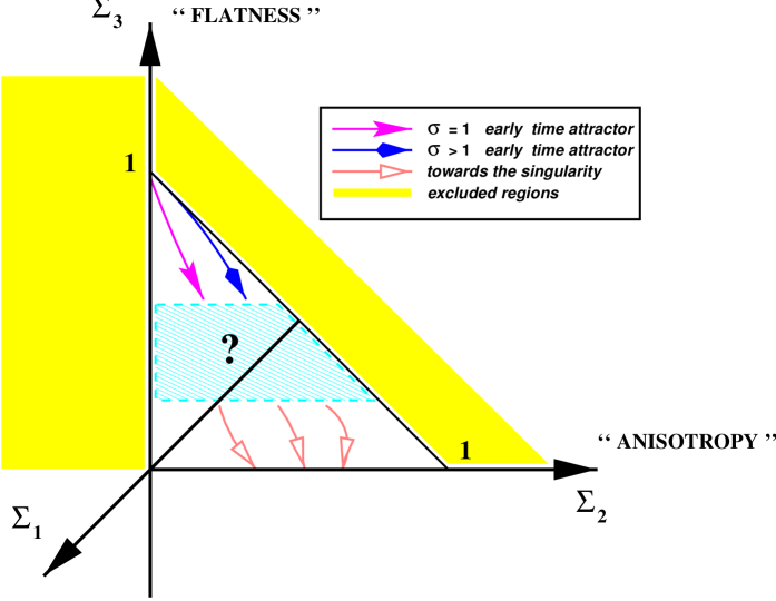
FIG. 1.: Approximate flow diagram from the early-time attractor to the singularity.

To evaluate the slope of the trajectories in the “flow diagram”, we will use Eqs. (102) and (103). Hence we get

$$\Upsilon_{1} \simeq \frac{1}{3}\,(\sum_{a}\alpha_{a})^{2}+\frac{2}{3}\,{\cal I}\,,$$ (145)

$$\Upsilon_{2} \simeq 1-\frac{1}{3}\,(\sum_{a}\alpha_{a})^{2}-\frac{2}{3}\,{\cal I}-\Gamma\,(t_{0}-t)^{2}\,,$$ (146)

$$\Upsilon_{3} \simeq \Gamma\,(t_{0}-t)^{2}\,,$$ (147)

where

$${\cal I}(t,\vec{x}) = \int^{t}_{t_{0}}dt^{\prime}\,(t_{0}-t^{\prime})\,\left\{\left[(\sum_{a}\alpha_{a})^{2}-\sum_{a}\alpha_{a}\right]\,(-R)+\right.$$ (149)

$$\left.\left[(\sum_{a}\alpha_{a})^{2}+\sum_{a}\alpha_{a}\right]\,(\nabla\varphi)^{2}-2(\sum_{a}\alpha_{a})^{2}g^{ij}\,\nabla_{i}\,\nabla_{j}\varphi\right\}\,.$$

Using the relations

$$\tilde{\chi}_{\,j}^{i}=e^{\varphi/2}\,(\chi_{\,j}^{i}-\delta^{i}_{\,j}\,\dot{\varphi})\,,$$ (150)

$$\tilde{R}=e^{\varphi}\,\left[R+2g^{ij}\,\nabla_{i}\,\nabla_{j}\varphi-\frac{1}{2}\,g^{ij}\,\partial_{i}\varphi\,\partial_{j}\varphi\right]\,,$$ (151)

we can express the Einstein-frame quantities $\Sigma_{1}$, $\Sigma_{2}$ and $\Sigma_{3}$ in terms of the string frame’s $\Upsilon_{1}$, $\Upsilon_{2}$ and $\Upsilon_{3}$. We get, in the super-inflationary PBB case,

$$\Sigma_{1} = \frac{3(1+\sqrt{3\Upsilon_{1}})^{2}}{(3+\sqrt{3\Upsilon_{1}})^{2}}\simeq\frac{3(1-\sum_{a}\alpha_{a})^{2}}{(3-\sum_{a}\alpha_{a})^{2}}-\frac{12(1-\sum_{a}\alpha_{a})}{(\sum_{a}\alpha_{a})(3-\sum_{a}\alpha_{a})^{3}}\,{\cal I}\,,$$ (152)

$$\Sigma_{2} = \frac{6\Upsilon_{2}}{(3+\sqrt{3\Upsilon_{1}})^{2}}\simeq\frac{2(3-(\sum_{a}\alpha_{a})^{2})}{(3-\sum_{a}\alpha_{a})^{2}}+\frac{12(1-\sum_{a}\alpha_{a})}{(\sum_{a}\alpha_{a})(3-\sum_{a}\alpha_{a})^{3}}\,{\cal I}-\frac{6\Gamma\,(t_{0}-t)^{2}}{(3-\sum_{a}\alpha_{a})^{2}}\,,$$ (153)

$$\Sigma_{3} = \frac{6\Upsilon_{3}}{(3+\sqrt{3\Upsilon_{1}})^{2}}\simeq\frac{6\Gamma\,(t_{0}-t)^{2}}{(3-\sum_{a}\alpha_{a})^{2}}\,.$$ (154)

Note that in a super-inflationary cosmological model ($\sum_{a}\alpha_{a}<0$) with negative three-curvature, if we are in a sufficiently isotropic region where $\sum_{a}\alpha_{a}<-1$ we have globally ${\cal I}<0$ and then the behaviour in time is

$$\Sigma_{1} \simeq \frac{3(1-\sum_{a}\alpha_{a})^{2}}{(3-\sum_{a}\alpha_{a})^{2}}-\Xi^{2}\,\log^{2}\left(1-\frac{t}{t_{0}}\right)\,\left(1-\frac{t}{t_{0}}\right)^{2-2{\rm Max}\,\alpha_{a}}\,,$$ (155)

$$\Sigma_{2} \simeq \frac{2(3-(\sum_{a}\alpha_{a})^{2})}{(3-\sum_{a}\alpha_{a})^{2}}+(\Xi^{2}-\Theta^{2})\,\log^{2}\left(1-\frac{t}{t_{0}}\right)\,\left(1-\frac{t}{t_{0}}\right)^{2-2{\rm Max}\,\alpha_{a}}\,,$$ (156)

$$\Sigma_{3} \simeq \Theta^{2}\,\log^{2}\left(1-\frac{t}{t_{0}}\right)\,\left(1-\frac{t}{t_{0}}\right)^{2-2{\rm Max}\,\alpha_{a}}\,.$$ (157)

Hence, we can conclude that $\delta\Sigma_{1},\delta\Sigma_{2}$ and $\Sigma_{3}$ are all of the same order in the limit $t\rightarrow t_{0}$, and the trajectories of the solutions in the flow diagram (see Fig. 1) can have any slope relative to the $\Sigma_{2}$ axis, depending on the values of $\Xi$ and $\Theta$.

V Summary and Discussion

We have been able to extend previous work by showing that, even in the presence of an antisymmetric-tensor/axion background, or of internal-dimension moduli, pre-big bang type inflation emerges naturally in string theory from generic initial perturbative data. Reasonably smooth initial patches inflate and keep becoming increasingly homogeneous and (spatially) flat, at least as long as the low-energy tree-level effective action description is valid.

We were able to estimate the duration of the perturbative pre-big bang phase and to show that it depends on two (arbitrary) classical moduli. A sufficient amount of inflation requires these moduli to be both bounded from above, something we do not believe has much to do with the concept of fine-tuning. The question remains open of whether higher-order ($\alpha^{\prime}$ or loop) corrections might deform the classical moduli space and allow a prediction for the duration of perturbative pre-big bang inflation.

We have also analysed the behaviour of our solutions towards the far past and argued in favour of the existence of a rather large basin of attraction towards a Milne-type Universe with trivial dilaton, axion and moduli. Since Milne’s Universe is equivalent to (a wedge of) Minkowski space-time, such a state is nothing but a disguised form of the exact perturbative vacuum of string theory. This result (which should be established on more rigorous grounds) leads to a striking confirmation of the viability of the basic pre-big bang postulate, stating that the Universe started its evolution from the trivial vacuum of string theory.

As we have shown in Section 4, such a state, being an early-time attractor, actually becomes a repulsor as we move forward in time, i.e. is classically unstable with respect to small fluctuations of the metric and of the dilaton–axion system. The generic cosmologies that spring out of the trivial vacuum consist of a quasi-Milne era, followed by an inflationary quasi-homogeneous pre-big bang era. The value of the string coupling and of the spatial curvature at the transition between the two phases are the two above-mentioned classical moduli.

Quite possibly, the most generic kind of string cosmology will be quite inhomogeneous in a global sense, since, a priori, the two moduli may take different values in different regions of space. As in chaotic inflation [20], homogeneity is a local property valid up to some scale determined by the size of the original patch, which gave rise to our observable Universe, and by the amount of inflation it suffered.

We finally recall that, once pre-big bang behaviour sets in, primordial vacuum fluctuations are parametrically amplified. Equivalently, in a particle-physics language, massless quanta are copiously produced by the time-dependent backgrounds. By the time the string coupling has grown to about its present value, these quanta are able to dominate the energy and to lead the Universe straight into the hot big bang era [23],[24].

Many points are still unclear throughout the picture, and much work is still needed, both on the topics discussed in this paper and on the issue of the transition from the pre-big bang to the FRW phase (the exit problem). However, the possibility that the hot big bang conditions—which we know to have prevailed some 15 billion years ago—simply emerged from the basic instability of the trivial (i.e. cold, empty, flat, free) vacuum of string theory appears to be gaining further credibility from the results reported here.

A

We will restrict ourselves to the case without axion and modulus fields.

Momentum constraints for $d=2$: Einstein frame

In the $2+1$ dimensional case we can choose the spatial coordinates in such a way as to make the “zweibeins” diagonal. Equations  (78) and (81) then become

$$\tilde{g}(\tilde{t},x,y)=e^{\tilde{\beta}_{i}(x,y)}\,\delta_{ij}\,\left(1-\frac{\tilde{t}}{\tilde{t}_{0}}\right)^{2\,\lambda_{i}(x,y)}\,,\quad\lambda_{1}(x,y)+\lambda_{2}(x,y)=1\,,$$ (A1)

$$\varphi(\tilde{t},x,y)=\varphi_{0}(x,y)-\sqrt{2}\,\sqrt{1-\lambda_{1}^{2}-\lambda_{2}^{2}}\,\log\left(1-\frac{\tilde{t}}{\tilde{t}_{0}}\right)\,,$$ (A2)

and for the “momentum” constraint, Eq. (73), we get (redefining $\lambda\equiv\lambda_{1}$ for simplicity)

$$\partial_{x}\lambda-(1-2\,\lambda)\,\partial_{x}\tilde{\beta}_{2} = (\partial_{x}\varphi_{0})\,\sqrt{\lambda-\lambda^{2}}\,,$$ (A3)

$$-\partial_{y}\lambda+(1-2\,\lambda)\,\partial_{y}\tilde{\beta}_{1} = (\partial_{y}\varphi_{0})\,\sqrt{\lambda-\lambda^{2}}\,.$$ (A4)

Note that the two equations are decoupled and that they can be solved for $\beta_{1}$ and $\beta_{2}$ by quadratures once $\lambda$ and $\varphi_{0}$ are given.

Momentum constraints for $d=2$: string frame

We now re-express the results of the previous section in the string frame in order to be able to discuss T-duality. The solutions (17) and (18) for the two-metric and the shifted dilaton are

$$g_{ij}(t,x,y)=e^{2\beta_{i}(x,y)}\,\delta_{ij}\,\left(1-\frac{t}{t_{0}}\right)^{2\,\alpha_{i}(x,y)}\,,\quad\alpha_{1}^{2}(x,y)+\alpha_{2}^{2}(x,y)=1\,,$$ (A5)

$$\overline{\varphi}(t,x,y)=\overline{\varphi}_{0}(x,y)-\log\left(1-\frac{t}{t_{0}}\right)\,.$$ (A6)

In the “momentum” constraints, Eq. (20), the leading terms as $t\rightarrow t_{0}$ automatically cancel and we get:

$$\partial_{x}(\alpha_{1}\,e^{-\overline{\varphi}_{0}})-e^{-\overline{\varphi}_{0}}\,(\alpha_{1}\,\partial_{x}\beta_{1}+\alpha_{2}\,\partial_{x}\beta_{2})=0\,,$$ (A7)

$$\partial_{y}(\alpha_{2}\,e^{-\overline{\varphi}_{0}})-e^{-\overline{\varphi}_{0}}\,(\alpha_{1}\,\partial_{y}\beta_{1}+\alpha_{2}\,\partial_{y}\beta_{2})=0\,.$$ (A8)

Introducing the function

$$\varphi_{0}(x,y)=\overline{\varphi}_{0}(x,y)+\beta_{1}(x,y)+\beta_{2}(x,y)$$ (A9)

Eqs. (A7) and (A8) become

$$\partial_{x}\beta_{2}=\frac{\partial_{x}\alpha_{1}-\alpha_{1}\partial_{x}\varphi_{0}}{\alpha_{2}-\alpha_{1}}\,,$$ (A10)

$$\partial_{y}\beta_{1}=\frac{\partial_{y}\alpha_{2}-\alpha_{2}\partial_{y}\varphi_{0}}{\alpha_{1}-\alpha_{2}}\,.$$ (A11)

Hence, also in the string frame, the “momentum” constraints are solved by quadratures provided $\varphi_{0}(x,y)$ and, say, $\alpha_{1}$ are used as inputs. Barring pathologies, we can always change the input $\alpha_{1}$ by a duality transformation (e.g. $\alpha_{1}\rightarrow-\alpha_{1}$) while keeping $\varphi_{0}(x,y)$ unchanged, and solve again in $\beta_{1}$, $\beta_{2}$, thus reconstructing the new $\overline{\varphi}_{0}(x,y)$. In this way we will arrive at a rather odd generalization of T-duality transformations in the asymptotic limit of the quasi-homogeneous case. It would be more natural to keep $\overline{\varphi}_{0}(x,y)$ rather than $\varphi_{0}(x,y)$ unchanged under duality, since this is what happens for the time-dependent parts, but then it is not clear how a solution can be explicitly constructed.

REFERENCES

• [1] R. Brandenberger and C. Vafa, Nucl. Phys. B316 (1989) 391.
• [2] G. Veneziano, Phys. Lett. B265 (1991) 287;
A.A. Tseytlin, Mod. Phys. Lett. A6 (1991) 1721;
A.A. Tseytlin and C. Vafa, Nucl. Phys. B372 (1992) 443;
A. Sen, Phys. Lett. B271 (1991) 295;
S.F. Hassan and A. Sen, Nucl. Phys. B375 (1992) 103;
M. Gasperini and G. Veneziano, Phys. Lett. B277 (1992) 256;
K.A. Meissner, Phys. Lett. B392 (1997) 298;
N. Kaloper and K.A. Meissner, Duality beyond the First Loop, CERN-TH/97-113, WATPHYS-THY-96/18 (hep-th/9705193).
• [3] K.A. Meissner and G. Veneziano, Phys. Lett. B267 (1991) 33; Mod. Phys. Lett. A6 (1991) 3397.
• [4] G. Veneziano, Ref. [2];
M. Gasperini and G. Veneziano, Astropart. Phys. 1 (1993) 317; Mod. Phys. Lett. A8 (1993) 3701; Phys. Rev. D50 (1994) 2519;
R. Brustein and G. Veneziano, Phys. Lett. B329 (1994) 429;
N. Kaloper, R. Madden and K.A. Olive, Nucl. Phys. B452 (1995) 677; Phys. Lett. B371 (1996) 34;
R. Easther, K. Maeda and D. Wands, Phys. Rev. D53 (1996) 4247;
E.J. Copeland, A. Lahiri and D. Wands, Phys. Rev. D51 (1995) 1569;
J.D. Barrow and K.E. Kunze, Phys. Rev. D55 (1997) 623; Inhomogeneous string cosmologies, SUSSEX-AST-97-1-2 (hep-th/9701085), to appear in Phys. Rev. D.
• [5] A continuously updated collection of papers on the PBB scenario is available at http://www.to.infn.it/teorici/gasperini/.
• [6] See, e.g. R. Poppe and S. Schwager, Phys. Lett. B393 (1997) 51;
A. Lukas, B.A. Ovrut and D. Waldram, Phys. Lett. B393 (1997) 65; String and M-theory cosmological solutions with Ramond forms UPR-723T (hep-th/9610238);
N. Kaloper, Phys. Rev. D55 (1997) 3394;
H. Lu, S. Mukherji and C.N. Pope, Phys. Rev. D55 (1997) 7926.
• [7] G. Veneziano, Inhomogeneous pre-big bang string cosmology, CERN-TH/97-42 (hep-th/9703150), to appear in Phys. Lett. B.
• [8] E.J. Copeland, A. Lahiri and D. Wands, Phys. Rev. D50 (1994) 4868.
• [9] M.S. Turner and E.J. Weinberg, Pre-big bang inflation requires fine tuning, FERMILAB-PUB-97-010-A (hep-th/9705035).
• [10] M. Gasperini, M. Maggiore and G. Veneziano, Nucl. Phys. B494 (1997) 315;
R. Brustein and R. Madden, Graceful exit and energy conditions in string cosmology, BGU-PH-97/06 (hep-th/9702043).
• [11] R. Brustein, M. Gasperini, M. Giovannini and G. Veneziano, Phys. Lett. B361 (1995) 45;
R. Brustein, M. Gasperini and G. Veneziano, Phys. Rev. D55 (1997) 3882;
A. Buonanno, M. Maggiore and C. Ungarelli, Phys. Rev. D55 (1997) 3330;
B. Allen and R. Brustein, Phys. Rev. D55 (1997) 3260;
M. Gasperini, Tensor perturbations in high-curvature string backgrounds, DFTT-23/97 (hep-th/9704045).
• [12] M. Gasperini, M. Giovannini and G. Veneziano, Phys. Rev. Lett. 75 (1995) 3796;
D. Lemoine and M. Lemoine, Phys. Rev. D52 (1995) 1955.
• [13] E.J. Copeland, R. Easther and D. Wands, Vacuum fluctuations in axion-dilaton cosmologies, SUSSEX-TH-97001 (hep-th/9701082) to appear in Phys. Rev. D;
E.J. Copeland, J.E. Lidsey and D. Wands, S-duality invariant perturbations in string cosmology, SUSSEX-TH-97-007 (hep-th/9705050).
• [14] A. Feinstein, R. Lazkoz and M.A. Vàzquez-Mozo, Closed inhomogeneous string cosmology, EHU-FT/9703 (hep-th/9704173).
• [15] M. Gasperini, R. Ricci and G. Veneziano, Phys. Lett. B319 (1993) 438;
E. Alvarez, L. Alvarez-Gaumé and Y. Lozano, Nucl. Phys. B424 (1994) 155;
S. Elitzur, A. Giveon, E. Rabinovici, A. Schwimmer and G. Veneziano, Nucl. Phys. B435 (1995) 147.
• [16] X.C. de la Ossa and F. Quevedo, Nucl. Phys. B403 (1993) 377.
• [17] J.D. Barrow and M.P. Dabrowski, Phys. Rev. D55 (1997) 630.
• [18] D.S. Goldwirth and T. Piran, Phys. Rep. 214 (1992) 223 and references therein;
A.D. Linde, D.A. Linde and A. Mezhlumian, Phys. Rev. D49 (1994) 1783;
G.L. Comer, N. Deruelle, D. Langlois and J. Parry, Phys. Rev D49 (1994) 2759;
N. Deruelle and D.S. Goldwirth, Phys. Rev. D51 (1995) 1563.
• [19] V.S. Mukhanov, private communication.
• [20] A. Linde, Phys. Lett. B129 (1983) 177.
• [21] E.A. Milne, Relativity, gravitation and world structure, Oxford University Press, London and New York (1935).
• [22] T. Tanaka and M. Sasaki, Phys. Rev. D55 (1997) 6061.
• [23] See, for instance, G. Veneziano, Helv. Phys. Acta 69 (1996) 553.
• [24] A. Buonanno, K.A. Meissner, C. Ungarelli and G. Veneziano, in preparation.