The Mixed Non-Abelian Coulomb Gas in Two Dimensions

Abstract

The statistical mechanics of a mixed gas of adjoint and fundamental representation charges interacting via 1+1-dimensional $U(N)$ gauge fields is investigated. In the limit of large $N$ we show that there is a first order deconfining phase transition for low densities of fundamental charges. As the density of fundamental charges becomes comparable to the adjoint charge density the phase transition becomes a third order one.

1 Introduction

The classical Coulomb gas is an important model in statistical mechanics. It is exactly solvable in one dimension. In two dimensions it exhibits the Berezinsky-Kosterlitz-Thouless phase transition which is the prototype of all phase transitions in two-dimensional systems which have $U(1)$ symmetry. In this paper, we shall discuss a generalization of the classical Coulomb gas to a system of quarks which interact with each other through non-Abelian electric fields. This model is known to be exactly solvable in some special cases, for $SU(2)$ gauge group and fundamental representation quarks in one dimension [1] and for $SU(N)$ gauge group in the large-$N$ limit with adjoint representation quarks in one dimension [2, 3]. It can also be formulated on the lattice and solved with adjoint quarks in the large $N$ limit in higher dimensions [3, 4] where it has a substantially more complicated structure, although, even there, a solution of some special cases of the model are relevant to the deconfinement transition of three and four-dimensional Yang-Mills theory [6].

In the present paper, we shall concentrate on solving a more general version of the one-dimensional model than has previously been considered and elaborating on the properties of the solution. The one-dimensional case has the advantage of being directly related to a continuum field theory, the heavy quark limit of 1+1-dimensional quantum chromodynamics (QCD). Part of the motivation for this work is to study the possibility of a confinement-deconfinement phase transition at high temperature or density in a field theory which has some of the features of QCD, i.e. with similar gauge symmetries and where interactions are mediated by non-Abelian gauge fields. QCD exhibits confinement at low temperature and density with elementary excitations being color neutral particles - mesons and baryons. On the other hand, at high temperature or high density it is very plausible that the dynamical degrees of freedom would be quarks and gluons - which would form a quark-gluon plasma, rather than the mesons and baryons of low temperature nuclear physics. At some intermediate temperature or density there should be a crossover between these two regimes. There are few explicitly solvable models where this behavior can be studied directly. Previous to the model of [2, 3], known explicit examples of phase transitions in Yang-Mills theory were not associated with confinement, but were either lattice artifacts [7] unrelated to the continuum gauge theory or were associated with topological degrees of freedom in Yang-Mills theory on the sphere [8] and cylinder [6, 9] and demark a finite range of coupling constants within which the gauge theory resembles a string theory.

In finite temperature Yang-Mills theory (or QCD with only adjoint quarks), confinement is thought to be governed by the realization of a global symmetry which is related to the center of the gauge group and implemented by certain topologically non-trivial gauge transformations that appear only at finite temperature [10, 11, 12, 13]. The Polyakov loop operator is an order parameter for spontaneous breaking of this center symmetry and yields a mathematical way of distinguishing the confining and deconfined phases. When fundamental representation quarks are present, the center symmetry is broken explicitly and the Polyakov loop operator is no longer a good order parameter for confinement. Whether, in this case, a mathematical distinction of confined and deconfined phases exists, and indeed whether there is a distinct phase transition at all, is an open question.

Here, we will consider a toy model which resembles two-dimensional QCD with heavy adjoint and fundamental representation quarks. It could also be thought of as the heavy quark limit of dimensionally reduced higher dimensional QCD where the adjoint particles are the gluons of the compactified dimension which get a mass (similar to a Debye mass) from the dimensional reduction, and the fundamental representation particles are the quarks. We will solve this model explicitly in the large-$N$ limit. The model with only adjoint quarks was solved in refs. [2, 3] and it was found that the explicit solution has a first order phase transition between confining and deconfining phases. These phases could be distinguished by the expectation value of the Polyakov loop operator, which provided an order parameter for confinement in that case. In this paper, we shall add fundamental representation quarks. Then, as in QCD, the center symmetry is explicitly broken and the Polyakov loop is always non-vanishing. We nevertheless find that the first order phase transition persists when the density of fundamental quarks is sufficiently small. When the density of fundamental quarks is increased until it is comparable to the density of adjoint quarks, the phase transition becomes a second order one. When the fundamental quark density is increased further, the phase transition is third order.

Another motivation of the present paper, as well as Ref. [2, 3] is to study a suggestion by Dalley and Klebanov [23] and Kutasov [14] that 1+1-dimensional adjoint QCD would be the simplest gauge theory model which exhibits some of the stringy features of a confining gauge theory. It is a long-standing conjecture that the confining phase of a gauge theory can be described by a string theory [15]. There are only two cases where this relationship is well understood, two-dimensional Yang-Mills theory [16, 17, 18, 19, 20] and compact quantum electrodynamics [21, 22]. At low temperatures 1+1-dimensional adjoint QCD is confining in the conventional sense that quarks only appear in the spectrum in color neutral bound states. This is a result of the fact that, in one dimension, the gluon field has no propagating degrees of freedom and therefore it cannot form a color singlet bound state with an adjoint quark. As a result, the quantum states are color singlet bound states of two or more adjoint quarks. The spectrum contains an infinite number of families of multi-quark bound states which resemble asymptotically linear Regge trajectories [14, 23, 24, 25] and, for large energies, the density of states increases exponentially with energy [26]. This implies a Hagedorn transition [27, 28, 29] at high temperature. Kutasov [14] supported this view by using an argument originally due to Polchinski [30] that a deconfinement transition occurs when certain winding modes become tachyonic at high temperature. This behaviour was a feature of the explicit first order deconfinement transition found in the model considered in [2, 3]. That model, which coincides with the heavy quark limit of adjoint QCD, is effectively a statistical mechanical model for strings of electric flux, with quarks attached to their ends.

The large-$N$ expansion of two-dimensional adjoint QCD has the same complexity as the large-$N$ expansion of a higher dimensional Yang-Mills theory and the leading order, infinite-$N$ limit cannot be found analytically [31]. In fact, the dimensional reduction of three or four-dimensional Yang Mills theory produces two-dimensional QCD with massless adjoint scalar quarks, so the combinatorics of planar diagrams is very similar.

1.1 Overview

This paper is organized as follows: In Section 2.1 we identify the gauged principal chiral model which corresponds to the gas with sources in various representations. In Section 2.2 the quantum mechanical formulation of this unitary matrix model is analyzed. This is followed by a section (2.3) where we rewrite the model in terms of collective variables (eigenvalue density), which are convenient for analyzing the large-$N$ limit.

Parametrized solutions to the collective field equations are given in Section 3.1, and the parametrized free energy and its derivatives are obtained in 3.2. We also show that they give rise to a first order differential equation the free energy has to obey. In Section 3.3 we establish the existence of a third order line in the phase diagram, and compute the point where it terminates. Using numerical techniques we show in 3.4 that the critical line continues from that point as a first order line. In Section 3.5 we discuss the phase diagram we obtained. The paper ends with a summary (Section 4).

2 Formalism

2.1 Effective action

The partition function of 1+1-dimensional Yang-Mills theory at temperature $T$ and coupled to a number $K$ of non-dynamical quarks at positions $x_{1}\ldots,x_{K}$ in representations $R_{1},\ldots,R_{K}$ of the gauge group is obtained by taking the thermal average of an ensemble of Polyakov loop operators

$$Z[T;x_{1},\ldots,x_{K};R_{1},\ldots,R_{K}]~{}=~{}\int dA_{\mu}~{}e^{-S[A]}~{}\prod_{i=1}^{K}{\rm Tr}{\cal P}e^{i\int_{0}^{1/T}d\tau A^{R_{i}}_{0}(\tau,x_{i})}\;,$$ (2.1)

where the Euclidean action is

$$S[A]~{}=~{}\int_{0}^{1/T}d\tau\int dx\frac{1}{2e^{2}}{\rm Tr}\left(F_{\mu\nu}(\tau,x)\right)^{2}\;,$$ (2.2)

the gauge fields are Hermitean $N\times N$ matrix valued vector fields which have periodic boundary conditions in imaginary time

$$A_{\mu}(\tau,x)=A_{\mu}(\tau+1/T,x)\;,$$

and the field strength is

$$F_{\mu\nu}\;\equiv\;\partial_{\mu}A_{\nu}-\partial_{\nu}A_{\mu}-i\left[A_{\mu},A_{\nu}\right]\;.$$

The gauge field can be expanded in basis elements of the Lie algebra $A^{R_{i}}_{\mu}\equiv A^{a}_{\mu}T^{a}_{R_{i}}$ with $T^{a}_{R_{i}}$ the generators in the representation $R_{i}$. For concreteness, we consider $U(N)$ gauge theory and denote the generators in the fundamental representation as $T^{a}$ with $a=1,\ldots,N^{2}$. They obey

$$\left[T^{a},T^{b}\right]\;=\;if^{abc}T^{c}\;,$$ (2.3)

normalized so that

$${\rm Tr}\;T^{a}T^{b}~{}=~{}\frac{1}{2}\delta^{ab}\;,$$ (2.4)

and with the sum rule

$$\sum_{a=1}^{N^{2}}T^{a}_{ij}T^{a}_{kl}~{}=~{}\frac{1}{2}\delta_{jk}\delta_{il}\;.$$ (2.5)

We remark that group elements $g^{Ad}$ in the adjoint representation are related to the fundamental representation matrices $g$ by

$$(g^{Ad})^{ab}\;=\;2\;\mbox{Tr}(g^{\dagger}T^{a}gT^{b})\;.$$ (2.6)

The expression (2.1) can be obtained by canonical quantization of 1+1-dimensional Yang-Mills theory with Minkowski space action coupled to some non-dynamical sources

$$S=-\int dtdx~{}\frac{1}{2e^{2}}{\rm Tr}F_{\mu\nu}F^{\mu\nu}~{}+~{}{\rm source~{}terms}\;.$$ (2.7)

In the following, we will review an argument for representing the partition function of Yang-Mills theory as a gauged principal chiral model which was first given in [36, 37] and which was generalized to the case of Yang-Mills theory with sources in [2, 3]. As is usual in canonical quantization of a gauge theory, the canonical conjugate $E(x)$ of the spatial component of the gauge field (which we denote by $A(x)$), is proportional to the electric field,

$$E\;=\;\frac{1}{e^{2}}F_{01}\;,$$

and obeys the commutation relation

$$\left[A^{a}(x),E^{b}(y)\right]~{}=~{}i\delta^{ab}\delta(x-y)\;.$$ (2.8)

The Hamiltonian is

$$H=\int dx~{}\frac{e^{2}}{2}\sum_{a=1}^{N^{2}}(E^{a}(x))^{2}\;.$$ (2.9)

This Hamiltonian must be supplemented by the Gauss’ law constraint equation which is the equation of motion for $A_{0}$ following from (2.7) and which contains the color charge densities of the sources

$${\cal G}^{a}(x)\equiv\left(\frac{d}{dx}E^{a}(x)-f^{abc}A^{b}(x)E^{c}(x)+\sum_{i=1}^{K}T^{a}_{R_{i}}\delta(x-x_{i})\right)\sim 0\ .$$ (2.10)

Here, the particles with color charges are located at positions $x_{1},\ldots,x_{K}$. $T^{a}_{R_{i}}$ are generators in the representation $R_{i}$ operating on the color degrees of freedom of the i’th particle.

There are two options for imposing this constraint. The first is to impose another gauge fixing condition such as

$$A~{}\sim~{}0\>,$$

and to use the constraints to eliminate both $E$ and $A$. The resulting Hamiltonian is

$$H=\sum_{i<j,a}\frac{e^{2}N}{4}T^{a}_{R_{i}}\otimes T^{a}_{R_{j}}\left|x_{i}-x_{j}\right|\;,$$ (2.11)

which was considered in Ref. [1]. It is the energy of an infinite range spin model where the spins take values in the Lie algebra of $U(N)$.

The other option, which makes the closest contact with string dynamics, is to impose the constraint (2.10) as a physical state condition,

$${\cal G}^{a}(x)~{}\Psi_{\rm phys}~{}=~{}0\;.$$

To do this, it is most illuminating to work in the functional Schrödinger picture, where the states are functionals of the gauge field, $\psi[A]$ and the electric field is the functional derivative operator

$$E^{a}(x)\Psi[A]~{}=~{}\frac{1}{i}\frac{\delta}{\delta A^{a}(x)}~{}\Psi[A]\;,$$

The time-independent functional Schrödinger equation is

$$\int dx\left(-\frac{e^{2}}{2}\sum_{a=1}^{N^{2}}\frac{\delta^{2}}{(\delta A^{a}(x))^{2}}\right)~{}\Psi^{a_{1}\ldots a_{K}}\left[A;x_{1},\ldots,x_{K}\right]~{}=~{}{\cal E}~{}\Psi^{a_{1}\ldots a_{K}}\left[A;x_{1},\ldots,x_{K}\right]\;.$$

Gauss’ law implies that the physical states, i.e. those which obey the gauge constraint (2.10), transform as

$$\Psi^{a_{1}\ldots a_{K}}\left[A^{g};x_{1},\ldots,x_{K}\right]\;\;=\;\;g^{\rm R_{1}}_{a_{1}b_{1}}(x_{1})\ldots g^{\rm R_{K}}_{a_{K}b_{K}}(x_{K})\;\Psi^{b_{1}\ldots b_{K}}\left[A;x_{1},\ldots,x_{K}\right]\;,$$

where

$$A^{g}\;\;\equiv\;\;gAg^{\dagger}-ig\nabla g^{\dagger}\;,$$

is the gauge transform of $A$.

For a fixed number of particles, the quantum mechanical problem is exactly solvable. For example, the wavefunction of a fundamental representation quark-antiquark pair is

$$\Psi^{ij}[A;x_{1},x_{2}]\;=\;\left({\cal P}e^{i\int_{x_{1}}^{x_{2}}dyA(y)}\right)^{ij}\;,$$ (2.12)

where the path ordered phase operator represents a string of electric flux connecting the positions of the quark and anti-quark. The energy is $\frac{e^{2}N}{4}|x_{1}-x_{2}|$. For a pair of adjoint quarks, the wavefunction is

$$\Psi^{ab}[A;x_{1},x_{2}]\;=\;{\rm Tr}\left(T^{a}{\cal P}e^{i\int_{x_{1}}^{x_{2}}A}T^{b}{\cal P}e^{i\int_{x_{2}}^{x_{1}}A}\right)\;.$$ (2.13)

with energy $\frac{e^{2}N}{2}|x_{2}-x_{1}|$. These energy states are identical to what would be obtained by diagonalizing the ‘spin’ operators in the gauge fixed Hamiltonian (2.11).

Note that the wavefunctions (2.12) and (2.13) are not normalizable by functional integration over $A$. This is a result of the fact that the gauge freedom has not been entirely fixed, so that the normalization integral still contains the infinite factor of the volume of the group of static gauge transformations.

In general, for a fixed distribution of quarks, a state-vector is constructed by connecting them with appropriate numbers of strings of electric flux so that the state is gauge invariant. The number of ways of doing this fixes the dimension of the quantum Hilbert space. If the flux strings overlap, the Hamiltonian can mix different configurations, so the energy eigenstates are superpositions of string configurations. However, this mixing is suppressed in the large-$N$ limit (i.e. the strings are non-interacting) and any string distribution is an eigenstate of the Hamiltonian with eigenvalue $(e^{2}N/4)\times$(total length of all strings).

We shall study the thermodynamics of this system by constructing the partition function. We work with the grand canonical ensemble and assume that the quarks obey Maxwell-Boltzman statistics. The partition function of a fixed number of quarks is constructed by taking the trace of the Gibbs density $e^{-H/T}$ over physical states. This can be implemented by considering set of all states in the representation of the commutator (2.8), spanned by, for example, the eigenstates of $A^{a}(x)$ and an appropriate basis for the quarks

$$|A\rangle\otimes e_{a_{1}}\otimes e_{a_{2}}\otimes\ldots\otimes e_{a_{K}}~{}~{}.$$

Projection onto physical, gauge invariant states is done by gauge transforming the state at one side of the trace and then integrating over all gauge transformations (and then dividing by the infinite volume of the gauge group) [35]. The resulting partition function is

$$Z[T/e^{2};x_{1},\ldots,x_{K}]\;=\;\int[dA][dg]~{}\left<A\right|e^{-H/T}\left|A^{g}\right>{\rm Tr}~{}g^{R_{1}}(x_{1})\ldots{\rm Tr}~{}g^{R_{K}}(x_{K})~{}~{},$$ (2.14)

where $[dg]$ is the Haar measure on the space of mappings from the line to the group manifold and $[dA]$ is a measure on the convex Euclidean space of gauge field configurations. The expression (2.14) is identical to (2.1) with the Polyakov loop operator is the trace of the group element $g(x)$ in the appropriate representation.

In going over to the grand canonical ensemble the first step is to integrate over all particle positions. We then multiply by the fugacities for each type of charge: a factor of $\lambda_{R}$ for each quark in representation $R$. To impose Maxwell-Boltzmann statistics, we divide by the factorial of the number of quarks in each representation. We then sum over all numbers of quarks in each representation. This exponentiates the fugacities, resulting in the grand partition function

$$Z[T/e^{2},\lambda_{R}]~{}=~{}\int[dA][dg]~{}e^{-S_{\rm eff}[A,g]}\;,$$ (2.15)

where the effective action is

$$\exp\Big{(}-S_{\rm eff}[A,g]\Big{)}=\left<A\right|e^{-H/T}\left|A^{g}\right>\exp\left(\int dx~{}\sum_{R}\lambda_{R}{\rm Tr}~{}g^{R}(x)\right)\;,$$ (2.16)

and the summation in the exponent is over all the irreducible representations of $U(N)$ we want to consider. The Hamiltonian is the Laplacian on the space of gauge fields. The heat kernel obeys the equation

$$\left(T^{2}\frac{\partial}{\partial T}+\int dx\frac{e^{2}}{2}\sum_{a=1}^{N^{2}}\left(\frac{\delta}{\delta A^{a}(x)}\right)^{2}\right)\left<A\right|e^{-H/T}\left|A^{g}\right>\;=\;0\;,$$

with the boundary condition

$$\lim_{1/T\rightarrow 0}\left<A\right|e^{-H/T}\left|A^{g}\right>\;\;=\;\;\delta(A-A^{g})\;.$$

These equations are easily solved by a Gaussian - divided by a $T$-dependent constant:

$$\left<A\right|e^{-H/T}\left|A^{g}\right>\;\;\sim\;\;\exp\left(-\int dx~{}\frac{T}{e^{2}}~{}{\rm Tr}~{}(A-A^{g})^{2}\right)\ .$$

We see that the effective theory is the gauged principal chiral model with a potential energy term for the group-valued degrees of freedom,

$$S_{\rm eff}[A,g]~{}=~{}\int dx~{}\left(\frac{N}{2\gamma}~{}{\rm Tr}\Big{|}\nabla g(x)+i[A(x),g(x)]\Big{|}^{2}-\sum_{R}\left(\lambda_{R}{\rm Tr}~{}g^{R}(x)\right)\right)\;.$$ (2.17)

Note that we have introduced the coupling constant

$$\gamma\;\;\equiv\;\;\frac{e^{2}\;N}{2T}\;.$$ (2.18)

When we analyze the limit $N\rightarrow\infty$, we will tune $e^{2}$ such that $\gamma$ is constant. Moreover, we assume that the fugacities $\lambda_{R}$ are scaled such that all terms in the action (2.17) are of order $N^{2}$.

The potential energy term in the effective action,

$$V(g)~{}\equiv~{}-\sum_{R}\lambda_{R}{\rm Tr}\left(g^{R}(x)\right)\;,$$ (2.19)

is the expansion of a local class function of the group element $g(x)$ (one which obeys $V(g)=V(hgh^{-1})$ for $h\in U(N)$) in group characters with coefficients $\lambda_{R}$. The characters

$$\chi_{R}(g)~{}\equiv~{}{\rm Tr}\left(g^{R}(x)\right)\;,$$

form a complete set of orthonormal class functions of the group variable, with inner product

$$\int[dg]\chi_{R}^{*}(g)\chi_{R^{\prime}}(g)~{}=~{}\delta_{R,R^{\prime}}\;.$$

Here [dg] is not a functional integral measure, but is the Haar measure for integration on $U(N)$. From the potential, we can find a fugacity by

$$\lambda_{R}~{}=~{}-\int[dg]\chi_{R}^{*}(g)V(g)\;.$$

By tuning the fugacities appropriately, we could obtain any local invariant potential.

The effective action (2.17) with all $\lambda_{R}=0$ was discussed by Grignani et.al. [36, 37] and was solved explicitly in the limit $N\rightarrow\infty$ by Zarembo [4, 5]. The model with $\lambda_{Ad}\neq 0$ (with adjoint quarks) was solved in Refs. [2] and [3]. The effective action (2.17) is gauge invariant,

$$S_{\rm eff}[A,g]~{}=~{}S_{\rm eff}[A^{h},hgh^{\dagger}]~{}~{}.$$

It is also covariant under the global transformation

$$S_{\rm eff}[A,zg,\lambda_{R}]~{}=~{}S_{\rm eff}[A,g,z^{-C_{1}(R)}\lambda_{R}]\;.$$ (2.20)

where $z$ is a constant element from the center of the gauge group, which for $U(N)$ is $\sim$ $U(1)$ and would be the discrete group $Z_{N}$ for gauge group $SU(N)$. Here, $C_{1}(R)$ is the linear Casimir invariant of the representation $R$, which is the number of boxes in the Young tableau corresponding to $R$. When the gauge group is $SU(N)$ and the only non-zero fugacities are for the zero ‘N-ality’ representations, i.e. those for which $C_{1}(R)=0$ mod $N$, there is a global $Z_{N}$ symmetry. For gauge group $U(N)$, this occurs only when all representations with non-zero fugacities have equal numbers of quarks and anti-quarks. The fugacities of other non-symmetric charges, can be thought of as an external field which breaks the center symmetry of the system explicitly. This situation is akin to the effect of an external magnetic field on a spin system.

2.2 Matrix quantum mechanics

If we re-interpret $x$ as Euclidean time, the partition function that we have derived has the form of a Euclidean space representation of the partition function for matrix quantum mechanics, where the free energy is identical to the ground state energy of the matrix quantum mechanics. We can study the latter model by mapping the problem to real time $\tau$ by setting $x=i\tau$ and $A\rightarrow-iA$. The action in real time is then

$$S_{QM}\;=\;\int d\tau\left(\frac{N}{2\gamma}{\rm Tr}\left|\dot{g}+i\left[A,g\right]\right|^{2}-V(g)\right)\;.$$

We remark that this action must not be confused with the action (2.2). $S_{QM}$ is the action for a 0+1-dimensional problem (quantum mechanics), while (2.2) is the action for Yang Mills theory in 1+1 dimensions. This remark also holds for the Hamiltonian below. In order to avoid confusion, we label the quantum mechanical quantities with the subscript $QM$.

The canonical momentum conjugate to the group valued position variable $g$ is the Lie algebra element

$$\Pi\;=\;\frac{N}{\gamma}\left(ig^{\dagger}\dot{g}+g^{\dagger}Ag-A\right)\;,$$

and the Hamiltonian is

$$H_{QM}\;=\;\frac{\gamma}{2N}{\rm Tr}\Pi^{2}-\frac{\gamma}{N}{\rm Tr}\Pi(g^{\dagger}Ag-A)~{}+~{}V(g)\;.$$ (2.21)

The gauge field $A$ plays the role of a Lagrange multiplier which enforces the constraint

$$g\Pi g^{\dagger}-\Pi\sim 0\;,$$

and the Hamiltonian reduces to

$$H_{QM}\;=\;\frac{\gamma}{2N}{\rm Tr}\Pi^{2}+V(g)\;.$$

We can expand the canonical momentum as

$$\Pi~{}=~{}\sum_{a}\Pi^{a}T^{a}\;,$$

Then, the components satisfy the Lie algebra

$$\left[\Pi^{a},\Pi^{b}\right]\; = \;if^{abc}\Pi^{c}\;,$$ (2.22)

$$\left[\Pi^{a},g\right]\; = \;gT^{a}\;,$$ (2.23)

$$\left[\Pi^{a},g^{\dagger}\right]\; = \;-T^{a}g^{\dagger}\;.$$ (2.24)

It follows that in the Schrödinger picture the components of the canonical momentum are represented as

$$\Pi^{a}~{}=~{}{\rm Tr}gT^{a}\frac{\partial}{\partial g}~{}=~{}g_{ij}T^{a}_{jk}\frac{\partial}{\partial g_{ik}}\;.$$

Denoted in components the constraint reads

$$G^{a}\;\equiv\;\left({\rm Tr}T^{a}gT^{b}g^{\dagger}-\frac{1}{2}\delta^{ab}\right)\Pi^{b}\sim 0\;.$$

The constraint has no operator ordering ambiguity. It generates the adjoint action of the symmetry group

$$\left[G^{a},g\right]\;=\;\frac{1}{2}\left[T^{a},g\right]\;.$$

The constraint can be realized as a physical state condition

$$G^{a}~{}\psi_{\rm phys}~{}=~{}0\;.$$

In the representation where states are functions of $g$, this implies that the physical states are class functions

$$\psi_{\rm phys}(g)~{}=~{}\psi_{\rm phys}(hgh^{-1})\;,$$

where $h\in U(N)$. This means that the physical states are functions of the eigenvalues of $g$. In a basis where $g$ is diagonal,

$$g~{}=~{}\left(\matrix{e^{i\alpha_{1}}&0&0&0&\ldots&0\cr 0&e^{i\alpha_{2}}&0&0&\ldots&0\cr 0&0&e^{i\alpha_{3}}&0&\ldots&0\cr 0&0&\ldots&&&0\cr 0&0&\ldots&&&e^{i\alpha_{N}}\cr}\right)\;,$$ (2.25)

the wavefunctions are functions of $\alpha_{i}$,

$$\psi_{\rm phys}(\alpha_{1},\ldots,\alpha_{N})=\psi_{\rm phys}(\alpha_{1},\ldots,\alpha_{i}+2\pi,\alpha_{N})\;.$$ (2.26)

Denoting the gauge group Laplacian in components

$$\triangle\;\;\equiv\;\;\sum_{a=1}^{N^{2}}(\Pi^{a})^{2}\;,$$ (2.27)

the Hamiltonian reads

$$H_{QM}\;\;=\;\;\frac{\gamma}{4N}\Delta\;+\;V(g)\;.$$

Since the potential $V(g)$ is also a class function and depends only on the eigenvalues, when operating on the physical states, the Hamiltionian can be expressed in terms of eigenvalues and derivatives by eigenvalues

$$H_{QM}\;=\;\frac{\gamma}{4N}\frac{1}{\tilde{J}(\alpha)}\left(\sum_{1}^{N}-\frac{\partial^{2}}{\partial\alpha_{i}^{2}}-N(N^{2}-1)/12\right)\tilde{J}(\alpha)+V(\alpha)\;,$$

where

$$\tilde{J}(\alpha)=\prod_{i<j}2\sin\frac{1}{2}(\alpha_{i}-\alpha_{j})=\frac{1}{(2i)^{N(N-1)/2}}\frac{J(\alpha)}{\prod_{i}z_{i}^{(N-1)/2}}\;,$$

and

$$J(z)=\prod_{i<j}(z_{i}-z_{j})~{}~{}~{},~{}~{}z_{i}\equiv e^{i\alpha_{i}}\;.$$

The physical states must by symmetric functions of $\alpha_{i}$. (There is a residual gauge invariance [38, 39] under the Weyl group which permutes the eigenvalues and the physical state condition requires that the physical states be symmetric under these permutations.) The normalization integral for the wavefunction is

$$\int[dg]\psi^{\dagger}(g)\psi(g)~{}=~{}1\;.$$

Since the integrand depends only on the eigenvalues of $g$, It is convenient to write the Haar measure as an integral over eigenvalues of $g$ with the Jacobian which is the Vandermonde determinant,

$$\int(\prod_{i}d\alpha_{i})|\tilde{J}(\alpha)|^{2}\psi^{\dagger}(\alpha)\psi(\alpha)~{}=~{}1\;.$$

The Hamiltonian and inner product have a particularly simple form when we redefine the wavefunction as

$$\tilde{\psi}(\alpha_{1},\ldots,\alpha_{N})\equiv\tilde{J}(\alpha)\psi(\alpha_{1},\ldots,\alpha_{N})\;.$$

Since $\tilde{J}$ is antisymmetric, $\tilde{\psi}$ is a completely antisymmetric function of the eigenvalues, which we can think of as the coordinates of fermions. The Hamiltonian is that of an interacting Fermi gas

$$\left\{\frac{\gamma}{4N}\left(\sum_{1}^{N}-\frac{\partial^{2}}{\partial\alpha_{i}^{2}}-N(N^{2}-1)/12\right)+V(\alpha)\right\}\tilde{\psi}(\alpha)={\cal E}\tilde{\psi}(\alpha)\;.$$

This correspondence of a c=1 matrix model with a Fermi gas was first pointed out in Ref. [40].

2.3 Large N: Collective variables

In this section we shall examine the collective field formulation of the large-$N$ limit of the theory that we discussed in the last subsection [4, 41, 42, 43]. The Hamiltonian obtained in the last subsection reads

$$H_{QM}\;\;=\;\;\frac{\gamma}{4N}\sum_{a=1}^{N^{2}}(\Pi^{a})^{2}\;+\;V(g)\;,$$ (2.28)

with (compare (2.19))

$$V(g)~{}\equiv~{}-\sum_{R}\lambda_{R}{\rm Tr}\left(g^{R}(\tau)\right)\;.$$

It was shown (compare (2.25),(2.26)) that the wavefunction depends only on the eigenvalues $e^{i\alpha_{j}}$ of $g$ and thus the density of eigenvalues

$$\rho(\theta,\tau)~{}\equiv~{}\frac{1}{N}\sum_{i=1}^{N}\delta(\theta-\alpha_{i}(\tau))\;,$$

completely characterizes the properties of the system. Interpretation of the physics of the system at large $N$ is more convenient when one considers the Fourier transform of the eigenvalue distribution

$$\rho(\theta,\tau)~{}=~{}\frac{1}{2\pi}~{}+~{}\frac{1}{2\pi}\sum_{n\neq 0}c_{n}(\tau)e^{-in\theta}\;,$$ (2.29)

where we have defined

$$c_{n}(\tau)\;\equiv\;\frac{1}{N}{\rm Tr}g^{n}(\tau)~{}~{}~{}~{},~{}~{}~{}c_{-n}(\tau)\;=\;\overline{c_{n}(\tau)}\;.$$

We now turn our attention to developing the collective field theory formulation of the (thermo-) dynamical problem given by the Hamiltonian (2.28). Since the wavefunction depends only on the eigenvalues of $g$, we would like a Hamiltonian equivalent to (2.28) but written in terms of the eigenvalue density $\rho$ and a conjugate momentum $\Pi$. At large $N$ we will find this Hamiltonian and write equations of motion for $\rho$ and $\Pi$. So far we have not imposed any restriction on the potential $V(g)$, but from now on we assume, that it can be expressed as a functional of the eigenvalue density $\rho(\theta)$. In particular the potential we are going to analyze below will have this property.

The canonical momentum operates on the wavefunction as

$$\Pi^{a}\psi[\rho]=\int d\theta\left[\Pi^{a},\rho(\theta)\right]\frac{\delta}{\delta\rho(\theta)}~{}\psi[\rho]$$

$$=\frac{1}{2\pi N}\int d\theta\sum_{K}e^{-iK\theta}K{\rm Tr}(T^{a}g^{K})\frac{\delta}{\delta\rho(\theta)}\psi[\rho]\;,$$

and the Laplacian (2.27) is

$$\Delta\psi[\rho]~{}=~{}\left(\frac{1}{4\pi N}\int d\theta\sum_{K}e^{-iK\theta}\left|K\right|\left(\sum_{L=0}^{K}{\rm Tr}g^{L}{\rm Tr}g^{K-L}-N{\rm Tr}g^{K}\right)\frac{\delta}{\delta\rho(\theta)}\right.$$

$$\left.+\;\frac{1}{8\pi^{2}N^{2}}\int d\theta d\theta^{\prime}\sum_{KL}KLe^{-iK\theta-iL\theta^{\prime}}{\rm Tr}g^{K+L}~{}\frac{\delta^{2}}{\delta\rho(\theta)\delta\rho(\theta^{\prime})}\right)~{}\psi[\rho]\;,$$

which can be written as

$$\Delta\psi[\rho]=-\frac{1}{2N}\int d\theta\rho(\theta)\Bigg{\{}\left(\frac{\partial}{\partial\theta}\frac{\delta}{\delta\rho(\theta)}\right)^{2}$$

$$-N^{2}{\cal P}\int d\theta^{\prime}\rho(\theta^{\prime})\cot\left(\frac{\theta-\theta^{\prime}}{2}\right)\frac{\partial}{\partial\theta}\frac{\delta}{\delta\rho(\theta)}\Bigg{\}}\psi[\rho]=$$

$$-\frac{1}{2N}\int d\theta\rho(\theta)\left(\left(\frac{\partial}{\partial\theta}\frac{\delta}{\delta\rho(\theta)}+{\cal V}(\theta)\right)^{2}-{\cal V}^{2}(\theta)\right)\psi[\rho]\;,$$

where

$${\cal V}(\theta)=\frac{N^{2}}{2}{\cal P}\int d\theta^{\prime}\rho(\theta^{\prime})\cot\left(\frac{\theta-\theta^{\prime}}{2}\right)\;.$$

${\cal P}$ indicates principal value integral.

The transformation of the wavefunction

$$\psi[\rho]\;=\;\tilde{\psi}[\rho]\exp\left(-\frac{N^{2}}{2}\int d\theta d\theta^{\prime}\ln\sin\frac{\left|\theta-\theta^{\prime}\right|}{2}\rho(\theta)\rho(\theta^{\prime})\right)\;,$$

transforms the derivative in the Schrödinger equation so that it has the form

$$\left\{-\frac{\gamma}{8N^{2}}\int d\theta\rho(\theta)\left\{\left(\frac{\partial}{\partial\theta}\frac{\delta}{\delta\rho(\theta)}\right)^{2}-{\cal V}^{2}(\theta)\right\}+V[\rho]\right\}~{}\tilde{\psi}[\rho]~{}=~{}E~{}\tilde{\psi}[\rho]\;.$$ (2.30)

The second term on the left-hand-side of this equation has a simple form. In [44] it is shown that it gives rise to a term which is cubic in the density. Thus, the Schrödinger equation has the form

$$\left\{-\frac{\gamma}{8N^{2}}\int d\theta\left(\rho(\theta)\left(\frac{\partial}{\partial\theta}\frac{\delta}{\delta\rho(\theta)}\right)^{2}-N^{4}\frac{\pi^{2}}{3}\rho^{3}(\theta)\right)+V[\rho]\right\}~{}\tilde{\psi}[\rho]~{}=~{}E~{}\tilde{\psi}[\rho]\;,$$ (2.31)

up to an overall constant.

The large-$N$ limit is dominated by the eikonal approximation. In this approximation, we make the ansatz for the wavefunction

$$\tilde{\psi}[\rho]~{}=~{}\exp\left(iN^{2}S[\rho]\right)\;.$$

The eikonal, $S$ then obeys the equation

$$\frac{H_{QM}[\rho,\Pi]}{N^{2}}~{}=~{}\frac{\gamma}{8}\int d\theta\left\{\rho(\theta)\left(\frac{\partial}{\partial\theta}\frac{\delta~{}S}{\delta\rho(\theta)}\right)^{2}+\frac{\pi^{2}}{3}\rho^{3}(\theta)\right\}+\frac{1}{N^{2}}V[\rho]~{}=~{}\frac{E}{N^{2}}\;.$$ (2.32)

Here, we have ignored a term which is of subleading order in $N^{2}$. We have also assumed that $V[\rho]$ will be of order $N^{2}$ (compare Section 2.1) and that the natural magnitude of the energy eigenvalue is of order $N^{2}$.

To solve this equation for the ground state, we must find its minimum by varying $\rho$ and the canonical momentum

$$\Pi\;=\;\delta S/\delta\rho\;,$$

subject to the condition that $\rho$ is normalized. This leads to the equations of collective field theory

$$\frac{\partial}{\partial\tau}\rho(\tau,\theta)\;\; = \;\;\frac{\;\delta H_{QM}/N^{2}\;}{\delta\Pi(\tau,\theta)}\;,$$

$$\frac{\partial}{\partial\tau}v(\tau,\theta)\;\; = \;\;-\frac{\partial}{\partial\theta}\;\frac{\;\delta H_{QM}/N^{2}\;}{\delta\rho(\tau,\theta)}\;,$$

where

$$v(\tau,\theta)~{}\equiv~{}\frac{\partial}{\partial\theta}\;\Pi(\tau,\theta)\;.$$

Taking the derivative of the second equation with respect to $\theta$ eliminates a Lagrange multiplier which must be introduced on order to enforce the normalization condition for $\rho$. Using (2.32) one finds

$$\frac{\partial}{\partial\tau}\rho\;+\;\frac{\gamma}{4}\frac{\partial}{\partial\theta}\left(\rho v\right)\; = \;0\;,$$

$$\frac{\partial}{\partial\tau}v\;+\;\frac{\gamma}{8}\frac{\partial}{\partial\theta}\left(v^{2}+\pi^{2}\rho^{2}\right)\;+\;\frac{1}{N^{2}}\frac{\partial}{\partial\theta}\frac{\delta}{\delta\rho}V[\rho]\; = \;0\;.$$ (2.33)

It is interesting to note that these are nothing but Euler’s equations for a fluid with equation of state $P=\pi^{2}\rho^{3}/3$ on a cylinder with coordinates $(\theta,\tau)$. The inclusion of a potential $V(\theta,\tau)$ corresponding to non-Abelian charges is equivalent to subjecting the fluid to an external force which is derived from $V(\theta,\tau)$.

We shall use these equations in the next section where we analyze the large-$N$ limit of a mixed gas of adjoint and fundamental charges.

3 Free energy and critical behaviour

3.1 Static solutions to the collective field equations

In this section we will find static solutions to the collective field equations (2.33). The most simple potentials involve only the lowest representations, the fundamental, its conjugate and the adjoint. We shall consider a slight generalization of these and use powers of the lowest representations to include multiple windings of the Polyakov loop operator. Our potential reads

$$V(g)\;\equiv\;-\sum_{n=1}^{\infty}\left(\kappa_{n}N{\rm Tr}(g^{n})+\bar{\kappa}_{n}N{\rm Tr}((g^{\dagger})^{n})+\lambda_{n}|{\rm Tr}g^{n}|^{2}\right)\;,$$ (3.1)

where we made use of (compare (2.5), (2.6))

$${\rm Tr}~{}(g^{Ad}(x))^{n}\;=\;\left|{\rm Tr}~{}g^{n}(x)\right|^{2}\;,$$

to relate the trace in the adjoint representation to the trace in the fundamental representation. The couplings for the fundamental representation charges (and their conjugates) were chosen to scale $\sim N$, to make the potential of order $N^{2}$. It should be remarked that parts of this section can easily be extended to more general potentials.

The potential (3.1) indeed can be expressed as a functional of the eigenvalue density (2.29). The collective field Hamiltonian (2.32) then reads

$$\frac{H_{QM}}{N^{2}}~{}=\frac{\gamma}{8}\int d\theta\left[\rho(\theta)\left(v(\theta)\right)^{2}+\frac{\pi^{2}}{3}\rho^{3}(\theta)\right]$$ (3.2)

$$-\sum_{n=1}^{\infty}\left(\lambda_{n}\left|\int d\theta~{}\rho(\theta)e^{in\theta}\right|^{2}+\kappa_{n}\int~{}d\theta~{}\rho(\theta)~{}{\rm e}^{in\theta}+\bar{\kappa}_{n}\int~{}d\theta~{}\rho(\theta)~{}{\rm e}^{-in\theta}\right)-\frac{\gamma}{96}\;.$$

In order to maintain correspondence with the original version of the Hamiltonian (2.28) we subtract the constant $\gamma/96$. It sets the energy scale such that the free energy vanishes in the confined phase of the model with only adjoint charges (see below).

The corresponding collective field equations (2.33) read

$$\frac{\partial\rho}{\partial x}\;+\;\frac{\gamma}{4}\frac{\partial}{\partial\theta}(\rho v)\;=\;0\;,$$ (3.3)

$$\frac{\partial v}{\partial x}\;+\;\frac{\gamma}{8}\frac{\partial v^{2}}{\partial\theta}\;-\;\frac{\pi^{2}\gamma}{8}\frac{\partial\rho^{2}}{\partial\theta}\;+\;\frac{\partial}{\partial\theta}\sum_{n}\left[(\lambda_{n}c_{-n}+\kappa_{n})~{}{\rm e}^{in\theta}+(\lambda_{n}c_{n}+\bar{\kappa}_{n})~{}{\rm e}^{-in\theta}\right]~{}=~{}0\;.$$ (3.4)

where $c_{n}$ are the $x$-dependent Fourier coefficients of $\rho$ as introduced in (2.29). Note that we also performed the change of variables, $\tau\rightarrow-ix$ and $v\rightarrow iv$ in these equations in order to invert the Wick rotation performed at the beginning of Section 2.2 prior to canonical quantization.

We will only consider real, static solutions of the non-linear equations (3.4), that is, where $\rho(\theta,x)=\rho_{0}(\theta)$ and the velocity $v$ vanishes identically. Consequently

$$\rho_{0}(\theta)=\left\{\matrix{2\sqrt{\frac{2}{\gamma\pi^{2}}}\sqrt{E+\sum(\lambda_{n}c_{-n}+\kappa_{n})e^{in\theta}+\sum(\lambda_{n}c_{n}+\bar{\kappa}_{n})e^{-in\theta}}&\mbox{where }\rho\mbox{ is real}\cr 0&{\rm otherwise}\cr}.\right.$$ (3.5)

The constant of integration $E$ has physical interpretation as the Fermi energy of a collection of $N$ fermions [40] in the potential $V[\rho]$ and is fixed by the normalization condition

$$1\;=\;\int d\theta~{}\rho_{0}(\theta)\;.$$ (3.6)

Here it is more convenient to express the $c_{n}$ in terms of $\rho_{0}$ (compare (2.29))

$$c_{n}\;=\;\int d\theta~{}\rho_{0}(\theta)e^{in\theta}\;.$$ (3.7)

The real support of the function $\rho_{0}(\theta)$ is the positive support of $\Lambda\equiv E+\sum(\lambda_{n}c_{-n}+\kappa_{n})e^{in\theta}+\sum(\lambda_{n}c_{n}+\bar{\kappa}_{n})e^{-in\theta}$. The zeros of $\Lambda$ define the edges of the eigenvalue distribution and when these zeros condense one has critical behaviour in the observables of the model as in general Hermitean and unitary matrix models.

3.2 A differential equation for the free energy

In this subsection we compute all first order derivatives of the free energy and show that they obey a differential equation of the Clairaut type.

Inserting the static solution (3.5) in (3.2) we obtain for the free energy

$$\frac{1}{N^{2}}\langle H_{QM}\rangle\;\;\equiv\;\;f\;\;=\;\;\frac{1}{3}E\;-\;\frac{1}{3}\sum_{n=1}^{\infty}\Big{[}\lambda_{n}|c_{n}|^{2}\;+\;2(\;\kappa_{n}c_{n}\;+\;\bar{\kappa}_{n}c_{-n}\;)\Big{]}-\frac{\gamma}{96}\;.$$ (3.8)

Note that $f$ is the leading coefficient ($O(N^{2})$) of the energy for the matrix quantum mechanics problem, but for the quark gas problem plays the role of the leading coefficient of the energy density.

Deriving the expression (3.8) with respect to $\lambda_{J}$ for some fixed $J$ and using derivatives of Equations (3.6) and (3.7) with respect to the same parameter one obtains

$$\frac{df}{d\lambda_{J}}\;=\;-|c_{J}|^{2}\;.$$ (3.9)

We use the notation $d/d\lambda_{J}$ to indicate that also the $c_{n}$ and $E$ which implicitly depend on $\lambda_{J}$ are derived with respect to this coupling. Similarly one can show

$$\frac{df}{d\kappa_{J}}\;=\;-c_{J}\;,$$ (3.10)

and

$$\frac{df}{d\gamma}\;=\;\frac{1}{3\gamma}E\;+\;\frac{1}{3\gamma}\sum_{n=1}^{\infty}\Big{[}2\lambda_{n}|c_{n}|^{2}\;+\;\kappa_{n}c_{n}\;+\;\bar{\kappa}_{n}c_{-n}\Big{]}\;-\;\frac{1}{96}\;.$$ (3.11)

It is interesting to notice, that combining Equations (3.9) - (3.11) gives rise to a first order differential equation of the Clairaut type

$$\gamma\frac{df}{d\gamma}\;+\;\sum_{n=1}^{\infty}\Big{[}\lambda_{n}\frac{df}{d\lambda_{n}}+\kappa_{n}\frac{df}{d\kappa_{n}}+\bar{\kappa}_{n}\frac{df}{d\bar{\kappa}_{n}}\Big{]}\;\;=\;\;f\;.$$ (3.12)

This differential equation has general solutions of the form

$$f(\gamma,\lambda_{n},\kappa_{n})\;\;=\;\;\gamma\;F(\frac{\lambda_{n}}{\gamma},\frac{\kappa_{n}}{\gamma})\;,$$

where $F$ is some arbitrary smooth function. This result shows that the parameter $\gamma$ is not driving the physical properties of the model, but rather sets the energy scale. The differential equation (3.12) gives no further restrictions on the function $F$ and another analysis will be adopted in the next section. However, when finding the physical interpretation of the phase diagram the differential equation (3.12) is a valuable tool.

3.3 Regime of the third order phase transition

We now restrict ourselves to the case of only one pair of non-vanishing couplings $\lambda_{J},\kappa_{J}\neq 0$. Furthermore it is sufficient to consider $\kappa_{J}$ real, since an eventual phase of $\kappa_{J}$ can always be removed by using the covariance (2.20) of the action and Haar measure $[dg]$ under transformations by a constant element of $U(1)$.

In the form of (3.5) it is evident we need to solve simultaneously for the normalization condition (3.6) and the Fourier moment (3.7) in order to have a self-consistent solution of the saddle-point equations. We begin by introducing an auxiliary complex parameter

$$r_{J}~{}e^{iJ\beta_{J}}\;\equiv\;\lambda_{J}~{}c_{-J}+\kappa_{J}\;,$$ (3.13)

and rescaling the Fermi energy as

$$E\;\;\equiv\;\;2\mu\;r_{J}\;.$$ (3.14)

With this notation the normalization and moment equations are respectively

$$1\;=\;2\sqrt{\frac{r_{J}}{\gamma}}\;I(\mu)\;\;\;\;\;\;,\;\;\;\;\;\;c_{J}e^{iJ\beta}\;=\;2\sqrt{\frac{r_{J}}{\gamma}}\;M(\mu)\;,$$ (3.15)

where we have defined the integrals

$$I(\mu)\; \equiv \;\frac{2}{\pi}\int_{-\pi}^{\pi}\sqrt{\mu+\cos(J\theta)}\;\mbox{H}(\mu+\cos(J\theta))\;d\theta\;,$$

$$M(\mu)\; \equiv \;\frac{2}{\pi}\int_{-\pi}^{\pi}\cos{J\theta}\sqrt{\mu+\cos(J\theta)}\;\mbox{H}(\mu+\cos(J\theta))\;d\theta\;.$$ (3.16)

Here H(..) denotes the step function. A simple transformation of the integration variable shows that $I(\mu)$ and $M(\mu)$ are independent of $J$. Thus $J$ enters only as the subscript of the parameters. For notational convenience we abbreviate

$$\lambda_{J}\;\equiv\;\lambda\;\;\;\;,\;\;\;\;\kappa_{J}e^{-iJ\beta_{J}}\;\equiv\;\kappa\;.$$ (3.17)

We remark that $I(\mu),M(\mu)$, and thus $c_{J}e^{iJ\beta_{J}}$ are real. Eliminating the moment $c_{J}$ from (3.15) by using the definition (3.13) we obtain

$$\frac{{\kappa}}{\gamma}\;\;=\;\;\frac{1}{I(\mu)^{2}}\left[\frac{1}{4}-\frac{\lambda}{\gamma}I(\mu)M(\mu)\right]\;.$$ (3.18)

This family of lines in the $\kappa,\lambda$-plane parametrized by $\mu$ represent a necessary condition which a solution of the normalization and moment equations (3.15) must obey. From the last equation it is obvious that also the product $\kappa\;=\;\kappa_{J}e^{-iJ\beta}$ is real (thus $e^{iJ\beta}$ is just a sign). It occurs as a natural parameter when rewriting the free energy in terms of $I(\mu)$ and $M(\mu)$ (use (3.8))

$$f\;=\;\frac{\gamma}{12I(\mu)^{2}}\left[2\mu-\frac{M(\mu)}{I(\mu)}\right]\;-\;\kappa\frac{M(\mu)}{I(\mu)}\;-\frac{\gamma}{96}\;,$$ (3.19)

where we have eliminated $\lambda$ using the necessary condition (3.18). Also the first derivative of the free energy with respect to $\kappa$ can be expressed conveniently in terms of $I(\mu)$ and $M(\mu)$

$$\frac{df}{d\kappa}\;=\;-2\frac{M(\mu)}{I(\mu)}\;.$$ (3.20)

Remember that we restricted ourselves to $\kappa_{J}$ real, and thus we encounter a factor 2 compared to 3.10), since a real $\kappa_{J}$ is the same for both terms $c_{J}$ and $c_{-J}$ in the potential (3.8).

With the parametric solution (3.8) at hand we turn our attention to establishing the critical behaviour in this model. In [44] it is shown that the first derivatives of $I(\mu)$ and $M(\mu)$ have non-analytic behaviour at $\mu=1$, hence the expression (3.20) suggests that the vicinity of $\mu=1$ is a natural place to look for non-analytic behaviour in the free energy of our model. Using the explicit results for $I(1),M(1)$ (see [44]) and (3.18) we obtain the necessary condition for the critical ($\mu=1$) values of $\lambda$ and $\kappa$

$$\frac{\kappa^{c}}{\gamma}\;\;=\;\;\frac{\pi^{2}}{512}\;-\;\frac{1}{3}\frac{\lambda^{c}}{\gamma}\;.$$ (3.21)

Having identified a line in the phase space where we expect critical behaviour we will now proceed to establish the details of this critical behaviour. Following [45, 46, 47] we begin by expanding about $\mu=1$ and the line (3.21)

$$\mu=1+\varepsilon,\varepsilon>0\;\;\;\;,\;\;\;\;I(1+\varepsilon)=I_{c}+\delta I\;\;\;\;,\;\;\;\;M(1+\varepsilon)=M_{c}+\delta M\;,$$ (3.22)

($I_{c}\equiv I(1),M_{c}\equiv M(1)$) and analyze the variation of $\kappa$ around $\kappa^{c}$ while keeping $\lambda$ fixed

$$\kappa=\kappa^{c}+\delta\kappa\;\;\;\;,\;\;\;\;\lambda=\lambda^{c}\;.$$ (3.23)

Due to the nontrivial support of the integrands in (3.16) in principle one has to distinguish the cases $\mu>1$ and $\mu<1$; (see [44] for details). In order to keep the formulas simple, we explicitly analyze only the case $\mu>1$ as given by (3.22), (3.23). The case $\mu<1$ can be treated along the same lines and we denote the corresponding results in the end.

The expansion now consists of two steps. We first expand the necessary condition (3.18) at $\mu=1$ to obtain the relation between the variation $\delta\kappa$ and $\varepsilon$. In the second step we expand the right hand side of (3.20) at $\mu=1$ and use the result of step one to express the variation of $df/d\kappa$ in terms of $\delta\kappa$. The latter result can then be used to analyze eventual singular behaviour of higher derivatives of the free energy.

Expanding the necessary condition (3.18) and using (3.21) we obtain for the variation of $\kappa$ to lowest order

$$\frac{\delta\kappa}{\gamma}\;\;\;=\;\;\;-\frac{1}{2}\frac{\delta I}{(I_{c})^{3}}\;-\;\frac{\lambda^{c}}{\gamma}\frac{M_{c}}{I_{c}}\left[\;\frac{\delta M}{M_{c}}-\frac{\delta I}{I_{c}}\right]\;\;\;=\;\;\;\left[\frac{-\pi^{2}}{256}+\frac{4}{3}\frac{\lambda^{c}}{\gamma}\right]\frac{\delta I}{I_{c}}\;\;-\;\;\frac{\lambda^{c}}{\gamma}\frac{\varepsilon}{2}\;,$$ (3.24)

where in the last step we made use of the relation between the variations $\delta I$ and $\delta M$ and inserted the explicit results for $I_{c}=I(1)$ and $M_{c}=M(1)$. Using the result for $\delta I/I_{c}$ to lowest order we obtain (see [44] for further details)

$$\delta\kappa\;\;=\;\;-\;\varepsilon\ln(\varepsilon)\;\sigma\;,$$ (3.25)

where we introduced the abbreviation

$$\sigma\;\equiv\;\frac{1}{8}\left[-\frac{\gamma\pi^{2}}{256}+\frac{4\lambda^{c}}{3}\right]\;.$$ (3.26)

Inverting equation (3.24) (again taking into account only the leading order) gives

$$\varepsilon\;=\;-\;\sigma^{-1}\delta\kappa\;\left[\ln\left(\sigma^{-1}\delta\kappa\right)\right]^{-1}\;.$$ (3.27)

This equation is the relation between the variation $\delta\kappa$ and $\varepsilon$ which is implied by the necessary condition (3.18). In the final step we expand the derivative of the free energy (3.20) at $\mu=1$ and use the result (3.27) to obtain the variation of the derivative in terms of $\delta\kappa$. Expanding (3.20) gives

$$\frac{df}{d\kappa}\;\;\;=\;\;\;-2\frac{M_{c}}{I_{c}}\left[1+\frac{\delta M}{Mc}-\frac{\delta I}{I_{c}}\right]\;\;\;=\;\;\;-\frac{2}{3}\;-\;\frac{1}{3}\varepsilon\ln(\varepsilon)\;-\;\varepsilon\;.$$ (3.28)

Using (3.27) we obtain

$$\frac{df}{d\kappa}\;\;\;=\;\;\;-\frac{2}{3}\;\;+\;\;\frac{1}{3}\sigma^{-1}\delta\kappa\;\;+\;\;\sigma^{-1}\delta\kappa\;\left[\ln\left(\sigma^{-1}\delta\kappa\right)\right]^{-1}\;.$$ (3.29)

We remark, that the case $\mu<1$ with expansion $\mu=1-\varepsilon,\;\varepsilon>0$ changes only the sign of the argument of the logarithm. Differentiating the last result with respect to $\delta\kappa$ establishes the singular behaviour of the third derivative of the free energy with respect to $\kappa$. Thus we find a third order phase transition for $\mu=1$. The critical line is a straight line given by (3.21).

It is important to notice, that at (see Equation (3.24))

$$\frac{\lambda^{c}}{\gamma}\;=\;\frac{3\pi^{2}}{1024}\;,$$ (3.30)

the leading term in the expression for $\delta\kappa$ vanishes. Equation (3.24) is reduced to the simpler relation

$$\frac{\delta\kappa}{\gamma}\;=\;-\varepsilon\;\frac{\lambda^{c}}{2\gamma}\;.$$ (3.31)

At this point the expansion of $df/d\kappa$ gives

$$\frac{df}{d\kappa}\;=\;-\frac{2}{3}\;-\;\frac{1}{3}\varepsilon\ln(\varepsilon)\;-\;\varepsilon\;=\;-\frac{2}{3}\;+\;\frac{2}{3\lambda^{c}}\delta\kappa\ln\left(-\frac{2}{\lambda^{c}}\delta\kappa\right)\;+\;\frac{2}{\lambda^{2}}\delta\kappa\;.$$ (3.32)

Again the case $\mu<1$ differs only by the sign of the argument of the logarithm. Differentiation with respect to $\delta\kappa$ shows, that the phase transition has turned to second order at that point. Using (3.21) one can compute also the $\kappa/\gamma$ coordinate of the second order point giving $\kappa/\gamma=\pi^{2}/1024,\lambda/\gamma=3\pi^{2}/1024$. In fact the more global analysis in the next section will show, that the third order line terminates at the second order point $\kappa/\gamma=\pi^{2}/1024,\lambda/\gamma=3\pi^{2}/1024$, and continues as a first order line.

3.4 Regime of the first order phase transition

As pointed out at the end of the last section at the point $\kappa/\gamma=\pi^{2}/1024$, $\lambda/\gamma=3\pi^{2}/1024$, the third order transition along the $\mu=1$ line (3.21) changes to second order. This unusual behaviour requires further investigation which we will carry out in this section. To begin, a graphical analysis of the phase diagram is most useful and in Figure 1 we plot a number of representatives of the family of lines (3.18) for a range of values of $\mu$.

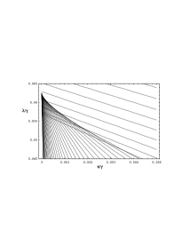
Figure 1: Plot of the lines (3.18) for $\mu$ ranging from $0.4$ (upper right corner) to $75$ (line at the extreme left). The region of overlapping lines corresponds to a region of first order phase transition.

It is clear that in most of the $\kappa,\lambda$-plane points are in a one-to-one correspondence with values of the parameter $\mu$. This correspondence breaks down though in a small region near the $\lambda/\gamma$ axis between $\lambda/\gamma=0.05$ and $\lambda/\gamma=0.0625$. Due to the behaviour of the slope and intercept in the linear equation (3.21) lines begin to overlap for increasing $\mu$ starting at $\mu\sim 1$ and continuing as $\mu\rightarrow\infty$. In this overlap region the phase diagram is folded at the vertex $\kappa/\gamma=\pi^{2}/1024$, $\lambda/\gamma=3\pi^{2}/1024$, and each point falls on three different lines of constant $\mu$. Consequently the system simultaneously admits three configurations with different free energies in this region of the phase space. This circumstance allows for a first order phase transition to develop along a line where the free energies of the different phases are equal.

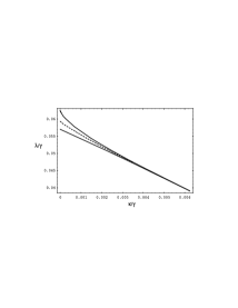
Figure 2: Plot of the boundary of the multiple phase region. The boundary (solid curve) is given by a caustic of lines in the one-parameter family (3.18). The dotted curve shows the numerically determined first order line.

The edges of the triangular first order region in Figure 1 is given by a caustic of lines from the one parameter family (3.18). The boundary is defined by the curve where the family of curves is stationary with respect to $\mu$. This condition can be used with (3.18) to give a definition of the boundary caustic shown in Figure 2. The stationary condition can be solved with the parametric result

$$\frac{\kappa}{\gamma}\;\;=\;\;\frac{1}{4I^{2}(\mu)}\;\frac{I^{\prime}(\mu)M(\mu)+M^{\prime}(\mu)I(\mu)}{M^{\prime}(\mu)I(\mu)-I^{\prime}(\mu)M(\mu)}\;.$$ (3.33)

As can be seen, the curve given by (3.33) intersects the $\lambda/\gamma$ axis at two points: $0.057024~{}(\mu=0.95324)$ and $1/16~{}(\mu=\infty)$ and reaches a singular maximum in the $\kappa/\gamma$ direction for $\mu=1$ at the point $\kappa/\gamma=\pi^{2}/1024$. The end of this region of first order transitions agrees with the position of the second order transition point which was determined by the analysis of critical behaviour in the previous section.

Once one has determined the region where different phases can co-exist the next issue to address is that of the position of the line of first order phase transitions where different phases have the same free energy.

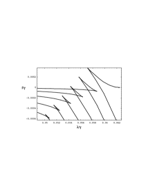
Figure 3: Free energy $f/\gamma$ as a function of $\lambda/\gamma$ in the region of first order phase transitions. Each curve is plotted for fixed $\kappa/\gamma$ which from right to left is $\kappa/\gamma=0,~{}0.0005,~{}0.001,~{}0.0015,~{}0.002,~{}0.0025$

The first order line can be determined for given $\kappa/\gamma$ by the simultaneous solution for the parameters $\mu_{1}$ and $\mu_{2}$ of the pair of equations

$$\frac{I(\mu_{2})M(\mu_{2})-I(\mu_{1})M(\mu_{1})}{4\;I(\mu_{1})I(\mu_{2})}\;=\;\frac{\kappa}{\gamma}\Big{[}M(\mu_{2})I(\mu_{1})-I(\mu_{2})M(\mu_{1})\Big{]}\;,$$ (3.34)

and

$$\frac{1}{6}\left(\frac{\mu_{1}}{I^{2}(\mu_{1})}-\frac{\mu_{2}}{I^{2}(\mu_{2})}\right)-\frac{1}{12}\left(\frac{M(\mu_{1})}{I^{3}(\mu_{1})}-\frac{M(\mu_{2})}{I^{3}(\mu_{2})}\right)\;=\;\frac{\kappa}{\gamma}\frac{I(\mu_{2})M(\mu_{1})-M(\mu_{2})I(\mu_{1})}{I(\mu_{1})I(\mu_{2})}\;.$$ (3.35)

Unfortunately, these equations are analytically intractable. Again we turn to a graphical analysis to gain further insight. In Figure 3 we plot the free energy of the system as a function of $\lambda/\gamma$ for different values of fixed $\kappa/\gamma$. From here it is easy to see a number of features of the region of first order transitions. Increasing $\mu$ traverses these curves in a clock-wise rotation so that the free energy increases for small values of $\mu$, intersecting the nearly horizontal large $\mu$ free energy. This intersection point is a graphical demonstration of the first order transition which occurs here as the model jumps from weak $(\mu<1)$ to strong coupling $(\mu$ large$)$. Each phase continues to exist after the transition point and may be reached by an adiabatic process until ending in cusps which mark the boundaries of the first order region in the $\lambda/\gamma$ axis. It is interesting to note that there is an energetically unfeasible intermediate “medium coupling” phase which connects the weak and strong phases. Hence, for fixed $\kappa/\gamma$ there exist three distinct configurations of the system for given $\lambda/\gamma$ in the region of first order transitions.

3.5 Phase diagram

We end this section with a short discussion of the phase diagram analyzed in the previous sections. Figure 4 shows a schematic picture of the phase diagram.

Figure 4: Schematic picture of the phase diagram. The dashed curve marks the first order part of the critical line. The solid curves above and below it are the boundaries of the area with two possible phases. They join at a point which shows second order behaviour. For larger $\kappa/\gamma$ we find a third order line ($\mu=1$) marked by a solid line. The numbers label four extremal corners of the phase diagram. We also indicate the range of the auxiliary parameter $\mu$.

The dashed line gives the numerically determined first order line. The full curves above and below show the boundaries of the region where different phases can coexist. With increasing $\kappa/\gamma$, this region narrows, and ends in a point which is second order as discussed above. The curve separating the two phases continues as the third order line (3.21).

We also show the range of the auxiliary parameter $\mu$. In the hot and dense (deconfining) phase it assumes values $\mu<1$, while in the cold and dilute (confining) phase it is restricted to $\mu>1$. On the third order part of the critical line we have $\mu=1$.

It is interesting to discuss the extremal regions of the phase diagram: In the case of only adjoint charges (all $k_{n}=0$) the action is invariant under transformations in the center of the gauge group, $g\rightarrow zg$ (compare (2.20)). When this symmetry is faithfully represented we expect

$$c_{n}(x)\;=\;\lim_{N\rightarrow\infty}\frac{1}{N}\langle{\rm Tr}~{}g^{n}(x)\rangle\;=\;0\;\;\;\;\;\;\forall n\neq 0\;,$$ (3.36)

since

$${\rm Tr}~{}g^{n}(x)~{}\rightarrow z^{n}~{}{\rm Tr}~{}g^{n}(x)\;.$$

From (3.3), (3.4) it is obvious that (3.36) which corresponds to constant eigenvalue density $\rho\equiv 1/2\pi$ is a solution. The stability analysis performed in [2] shows that this solution (”confined phase”) is stable for $\lambda/\gamma\in[0,1/16]$. Since the upper boundary of the multiple phase region is at $\lambda/\gamma=1/16$ we confirm this result.

The center symmetry of the action is explicitly broken when there are fundamental charges (some $\kappa_{n}\neq 0$). In particular this is the case when we consider the model with only fundamental charges (and their conjugate). Thus we cannot expect to find a confining solution with vanishing $c_{n}$ which would correspond to vanishing (energy) densities of colour electric string $(\rho_{Flux})$, fundamental representation charges $(\rho_{F,\bar{F}})$ and adjoint representation charges $(\rho_{Ad})$ (please see [44] for details). For this case ($\lambda=0$) we have established the existence of a third order phase transition at $\kappa/\gamma=\pi^{2}/512$ (set $\mu=1,\lambda=0$ in (3.18)).

Finally we discuss extremal corners of the phase diagram, which are labeled 1,..,4 in Figure 4. The four extremal cases can easily be understood by the magnitude of the energy densities $\rho_{Flux}$, $\rho_{Ad}$ and $\rho_{F,\bar{F}}$. Point 1 is in the extremal corner of the low density phase. All three densities are rather small. Points 2 and 3 are both in the high density phase, in areas which are dominated by adjoint charges (Point 2) and fundamental charges (Point 3). It is nice to see, how the energy density of the sources is dominated by the contributions of the adjoint charges and fundamental charges respectively. Finally Point 4 is in a region where both the density of the adjoint charges as well as the fundamental charges is high and of the same magnitude.

4 Summary

In this paper we analyzed the thermodynamic properties of a model of static sources on a line interacting through non-Abelian forces. It was shown that the partition function takes the form of the partition function of a gauged principal chiral model. Using the eigenvalue density as collective field variable the Hamiltonian for the eigenvalue density in the large $N$-limit was computed. We gave a static solution of the corresponding Hamilton equations. For the special case of only two types of charges, the static solution was parametrized using the parameter $\mu$ proportional to the Fermi energy. In particular the case of two types of charges transforming under the adjoint, and charges transforming under the fundamental representation of the gauge group was considered. Expanding the parametrized solutions at $\mu=1$ we established the existence of a straight line in the phase diagram where the free energy exhibits a third order phase transition. We proved that the third order behaviour terminates at a second order point. The critical line then continues as a first order line, which was determined numerically.

The whole phase diagram was interpreted by analyzing the contributions of charges and flux to the energy density. We found that for $\mu>1$ the system is characterized by low energy densities, while for $\mu<1$ the densities are high.

This 2-dimensional model could be generalized in several directions. It would be interesting to analyze non-static solutions of the Hamilton equations and different boundary conditions which might be used to include a $\theta$-term. Loop expansion of the fermion determinant of QCD₂ with large quark masses could be used to relate the fugacities of the non-Abelian gas analyzed in this article to the mass parameters of QCD₂.

Acknowledgment

This work was supported in part by the Natural Sciences and Engineering Research Council of Canada. L. P. is supported in part by a University of British Columbia Graduate Fellowship.

References

References

- [1] Y. Nambu, B. Bambah and M. Gross, Phys. Rev. D26, 2875 (1982).
- [2] G. W. Semenoff, O. Tirkkonen and K. Zarembo, Phys. Rev. Lett. 77, 2174 (1996); (hep-th/9605172).
- [3] G. W. Semenoff and K. Zarembo, Nucl. Phys. B480, 317 (1996); (hep-th/9606117).
- [4] K. Zarembo, Mod. Phys. Lett. A10, 677 (1995); (hep-th/9405080).
- [5] K. Zarembo, Teor. i Mat. Fiz. 104, 25 (1995).
- [6] M. Billo, M. Caselle, A. D’Adda and S. Panzeri; Int. J. Mod. Phys. A12, 1783 (1997); (hep-th/9610144).
- [7] D. Gross and E. Witten, Phys. Rev. D21, 446 (1980).
- [8] M. Douglas and V. Kazakov, Phys. Lett. 319B, 219 (1993); (hep-th/9305047).
- [9] D. Gross and A. Matytsin, Nucl. Phys. B437, 541 (1995); (hep-th/9410054).
- [10] A. M. Polyakov, Phys. Lett. 72B, 477 (1978).
- [11] L. Susskind, Phys. Rev. D20, 2610 (1979).
- [12] B. Svetitsky and L. Yaffe, Nucl. Phys. B210, 423 (1982).
- [13] B. Svetitsky, Phys. Rept. 132, 1 (1986).
- [14] D. Kutasov, Nucl. Phys. B414, 33 (1994); (hep-th/9306013).
- [15] A. M. Polyakov, Gauge Fields and Strings, (Harwood Academic Publishers, Chur, Switzerland, 1987).
- [16] V. Kazakov, Soviet Physics JETP 58, 1096 (1983).
- [17] I. Kostov, Nucl. Phys. B265, 223 (1986).
- [18] D. Gross, Nucl. Phys. B400, 161 (1993); (hep-th/9212149).
- [19] D. Gross and W. Taylor, Nucl. Phys. B400, 181 (1993); (hep-th/9301068).
- [20] D. Gross and W. Taylor, Nucl. Phys. B403, 395 (1993); (hep-th/9303046).
- [21] A. M. Polyakov; Nucl. Phys. B486, 23 (1997); (hep-th/9607049).
- [22] A. M. Polyakov, Lectures at Banff Summer School on Particles and Fields, (July 1994, unpublished).
- [23] S. Dalley and I. Klebanov, Phys. Rev. D47, 2517 (1993); (hep-th/9209049).
- [24] G. Bhanot, K. Demeterfi and I. Klebanov, Phys. Rev. D48, 4980 (1994); (hep-th/9307111).
- [25] D. Demeterfi, G. Bhanot and I. Klebanov, Nucl. Phys. B418, 15 (1994); (hep-th/9311015).
- [26] I. Kogan and A. Zhitnitsky, Nucl. Phys. B465, 99 (1996); (hep-ph/9509322).
- [27] R. Hagedorn, Nuovo Cimento Suppl. 3, 147 (1965).
- [28] S. Fubini and G. Veneziano, Nuovo Cimento 64A, 1640 (1969).
- [29] K. Huang and S. Weinberg, Phys. Rev. Lett. 25, 895 (1970).
- [30] J. Polchinski, Phys. Rev. Lett. 68, 1267 (1992); (hep-th/9109007).
- [31] G. t’Hooft, Nucl. Phys. B72, 461 (1974).
- [32] N. Weiss, Phys. Rev. D35, 2495 (1987).
- [33] A. Roberge and N. Weiss, Nucl. Phys. B275, 734 (986).
- [34] O. Borisenko, M. Faber and G. Zinoviev; Mod. Phys. Lett. A12, 949 (1997); (hep-lat/9604020).
- [35] D. Gross, R. Pisarski and L. Yaffe, Rev. Mod. Phys. 53, 43 (1981).
- [36] G. Grignani, G. W. Semenoff and P. Sodano, Phys. Rev D53, 7159 (1996); (hep-th/9504105).
- [37] Grignani, G. W. Semenoff, P. Sodano and O. Tirkkonen, Int. J. Mod. Phys. A11, 4103 (1996); (hep-th/9511110); Nucl. Phys. B473, 143 (1996); (hep-th/9512048).
- [38] E. Langmann and G. Semenoff, Phys. Lett. B296, 117 (1992); (hep-th/9210011).
- [39] E. Langmann and G. Semenoff, Phys. Lett. B303, 303 (1993); (hep-th/9212038).
- [40] E. Brezin, C. Itzykson, G. Parisi and J.-B. Zuber, Commun. Math. Phys. 59, 35 (1979).
- [41] A. Jevicki and B. Sakita, Phys. Rev. D22, 467 (1980).
- [42] S.R. Wadia, Phys. Lett. 93B, 403 (1980).
- [43] S.R. Das and A. Jevicki, Mod. Phys. Lett. A5, 1639 (1990).
- [44] C.R. Gattringer, L.D. Paniak and G.W. Semenoff, Ann. of Phys. 256, 74 (1997); (hep-th/9612030).
- [45] S. Gubser and I. Klebanov, Phys. Lett. B340, 35 (1994); (hep-th/9407014).
- [46] F. Sugino and O. Tsuchiya, Mod. Phys. Lett. A9, 3149 (1994); (hep-th/9403089).
- [47] I. Klebanov and A. Hashimoto, Nucl. Phys. B434, 264 (1995); (hep-th/9409064).
- [48] S.R. Das, A. Dhar, A.M. Sengupta and S.R. Wadia, Mod. Phys. Lett. A5, 891 (1990).
- [49] J. Bricmont and J. Fröhlich, Phys. Lett. 122B, 73 (1983).
- [50] K. Fredenhagen and M. Marcu, Phys. Rev. Letters 56, 233 (1986).
- [51] J. Spanier and K.B. Oldham, An Atlas of Functions, (Hemisphere Publishing Company, New York, 1987).