Soliton scattering in the $O(3)$ model on a torus

Abstract

Using numerical simulations, the stability and scattering properties of the $O(3)$ model on a two-dimensional torus are studied. Its solitons are found to be unstable but can be stabilized by the addition of a Skyrme-like term to the Lagrangian. Scattering at right angles with respect to the initial direction of motion is observed in all cases studied. The model has no solutions of degree one, so when a field configuration that resembles a soliton is considered, it shrinks to become infinitely thin. A comparison of these results with those of the model defined on the sphere is made.

1 Introduction

The non-linear $O(3)$ model in two dimensions appears as a low dimensional analogue of non-abelian gauge field theories in four dimensions. This analogy relies on common properties like conformal invariance, non-trivial topology, existence of solitons, hidden symmetries and asymptotic freedom. Among various applications, the $O(3)$ model has been used in the study of the quantum Hall effect and in models of high-$T_{c}$ superconductivity. In solid state physics it arises as the continuum limit of an isotropic ferromagnet, and in differential geometry the solutions of the model are known as harmonic maps.

The classical $O(3)$ model defined on the sphere, or on compactified plane, has been amply discussed in the literature [1, 2]. Its finite-energy solutions are static solitons or instantons describing lumps of energy. The model in three dimensional space-time is not integrable, and so to study the time evolution of its solitons one must resort to numerical simulations. The stability of the solitons has been analyzed in reference [3]. Due to the conformal invariance of the theory in two spatial dimensions, these soliton-like lumps are unstable in the sense that they change their size under any small perturbation, either explicit or introduced by the discretization procedure. When the lumps collide head-on, they scatter in general at 90^∘ to the initial direction of motion in the center-of-mass frame [4, 5]. Some time after the collison the instability of the solitons makes them shrink at an ever-increasing rate and they become so spiky that the numerical simulations break down. However, it has been shown [5, 6] that this instability of the model can be cured by the addition of two extra terms to the Lagragian. The first one resembles the term introduced by Skyrme in his nuclear model in four dimensional space-time [7], and the second one is an additional potential term. The solitonic solutions of this modified model are stable lumps (skyrmions) which repel each other and scatter at 90^∘ when sent towards each other with sufficient speed.

In the present paper we study the evolution properties of the $O(3)$ model when periodic boundary conditions are imposed; this amounts to defining the classical model on a two-dimensional torus. This approach looks more physical than the one on the sphere in the sense that the solitons are located in a finite volume from the outset. In any case, a comparison between both the toroidal and the spherical approaches is certainly of interest, if only to check the consistency of the two results.

In the next section we present the $O(3)$ model on the torus, and explain the numerical set up in the following one. Solitons of degree one in both the $O(3)$ scheme and its Skyrme version are discussed in section 4, whereas their scattering is studied in section 5. Section 6 completes our paper with some conclusions.

2 The $O(3)$ model on the torus

The non-linear $O(3)$ model involves three real scalar fields $\vec{\phi}(x^{\mu})\equiv\{\phi_{a}(x^{\mu}),a=1,2,3\}\,$ with the constraint that for all $x^{\mu}\equiv(x^{0},x^{1},x^{2})=(t,x,y)$ the fields lie on the unit sphere $S_{2}$:

$$\vec{\phi}.\vec{\phi}=1.$$ (1)

Subject to the above constraint the Lagrangian density and the corresponding equations of motion read

$${\cal L}=\frac{1}{4}(\partial_{\mu}\vec{\phi}).(\partial^{\mu}\vec{\phi}),$$ (2)

$$\partial^{\mu}\partial_{\mu}\vec{\phi}+(\partial^{\mu}\vec{\phi}.\partial_{\mu}\vec{\phi})\vec{\phi}=\vec{0}.$$ (3)

For any value of $t$, the fields $\vec{\phi}$ are mappings from the torus $T_{2}$ to the sphere $S_{2}$, i.e., they satisfy the periodic boundary conditions

$$\vec{\phi}(x+mL,y+nL)=\vec{\phi}(x,y),$$ (4)

where $m,n=0,1,2,...,$ and the period $L$ denotes the size of the square torus.

It is convenient to describe the model in terms of one independent complex field $W$, related to $\vec{\phi}$ via

$$\vec{\phi}=(\frac{W+\bar{W}}{|W|^{2}+1},i\frac{-W+\bar{W}}{|W|^{2}+1},\frac{|W|^{2}-1}{|W|^{2}+1}).$$ (5)

Introducing complex coordinates $z=x+iy$ and $\bar{z}=x-iy$ on the torus and using the handy notation $\partial_{z}W=W_{z},\,\partial_{z}(\partial_{\bar{z}}W)=W_{z\bar{z}}$, etc., the equation of motion (3) for the static field configurations becomes

$$W_{z\bar{z}}-\frac{2\bar{W}W_{z}W_{\bar{z}}}{|W|^{2}+1}=0,$$ (6)

whereas the boundary conditions (4) take the form

$$W(z+mL+inL)=W(z).$$ (7)

Whence, our static solitons or instantons are elliptic functions that may be expressed as [8]

$$W=\lambda\prod_{j=1}^{\kappa}\frac{\sigma(z-a_{j})}{\sigma(z-b_{j})},$$ (8)

with the zeros $(a_{j})$ and poles $(b_{j})$ subject to the selection rule

$$\sum_{j=1}^{\kappa}a_{j}=\sum_{j=1}^{\kappa}b_{j}.$$ (9)

The complex number $\lambda$ is related to the size of the soliton and $\kappa$ is the order of the elliptic function $W$. The Weierstrass $\sigma$-function is defined on $T_{2}$ and satisfies the pseudo-periodicity property [8]

$$\sigma(z+mL+inL)=(-1)^{(m+n+mn)}\exp(\frac{\pi}{L}(m-in)[z+\frac{1}{2}(m+in)L])\sigma(z).$$ (10)

For a square torus we have the so-called lemniscatic case, where $\sigma$ posseses a Laurent expansion of the form

$$\sigma(z)=\sum_{j=1}^{\infty}{c}_{j}z^{4j+1},$$ (11)

where the real coefficients ${c}_{j}$ depend on $L$.

Note that the periodicity of the torus means that our study can be simplified to the consideration of the system in a fundamental cell delimited by the vertices

$$(0,0),\,(L,0),\,(L,L),\,(0,L).$$ (12)

We are interested in static finite-energy solutions, which in the language of differential geometry are harmonic maps $T_{2}\rightarrow S_{2}$. These maps have been extensively studied in differential geometry [9, 10]. They are partitioned into homotopy sectors parametrized by an invariant integral index $Q$, the degree of the map, defined as usual by taking a two-form from $S_{2}$ to $T_{2}$ via the pull back map $W^{*}$. For a given map $W:T_{2}\rightarrow S_{2}$ we can pull back the Kahler form

$$\omega=4i\frac{d\xi\wedge d\bar{\xi}}{(1+\xi\bar{\xi})^{2}},\qquad\xi\,\epsilon\,S_{2},$$ (13)

and define

$$Q=\frac{1}{C}\int_{T_{2}}W^{*}\omega,$$ (14)

where the constant $C$ normalizes $Q$ to an integer. Expanding (13) in terms of $z$ and setting $C=-8\pi$ we obtain

$$Q=\frac{1}{\pi}\int_{T_{2}}\frac{|W_{z}|^{2}-|W_{\bar{z}}|^{2}}{(|W|^{2}+1)^{2}}\,dxdy.$$ (15)

The potential energy $V$, as derived from the Lagrangian (2), and the topological index satisfy

$$V\geq 2\pi|Q|.$$ (16)

The instanton-solutions correspond to the equality in (16): Solutions carrying $Q>0$ $(Q<0)$ imply $W_{\bar{z}}=0$ $(W_{z}=0)$, which are the Cauchy-Riemann conditions for $W$ being an analytic function of $z$ $(\bar{z})$.

The periodic solitons (8) have been studied in a variety of contexts. In reference [11], for example, they were used to compute the contribution of instantons to the partition function.

3 Numerical procedure for the time evolution

So far we have discussed the static field configurations. Now we concentrate on their dynamics, paying particular attention to their stability, scattering properties, etc.. As our model is not integrable, the study of the evolution of our fields requires numerical techniques. Hence, we treat configurations (8)-(9) as initial conditions for our evolution, studied numerically. The field $\vec{\phi}$ is evolved according to the equation of motion (3). We compute the series (11) up to the fifth term, the coefficients ${c}_{j}$ being in our case negligibly small for $j\geq 6$. The numerical set up is similar to that used in our previous papers (see [12] for example): We employ the fourth-order Runge-Kutta method and approximate the spatial derivatives by finite differences. The Laplacian is evaluated using the standard nine-point formula and, to further check our results, a 13-point recipe is also utilized. We work on a 200x200 periodic lattice ($n_{x}=n_{y}=200$) with spatial and time steps $\delta x$=$\delta y$=0.02 and $\delta t$=0.005, respectively. The size of our torus is then $L=n_{x}\times\delta x=4$.

Unavoidable numerical truncation errors introduced at various stages of the calculations gradually shift the fields away from the unit sphere (1). So we rescale

$$\vec{\phi}\rightarrow\vec{\phi}/\sqrt{\vec{\phi}.\vec{\phi}}$$

every few iterations. The error associated with this procedure is of the order of the accuracy of our calculations. Each time, just before the rescaling operation, we evaluate the quantity $\mu\equiv\vec{\phi}.\vec{\phi}-1$  at each lattice point. Treating the maximum of the absolute value of $\mu$ as a measure of the numerical errors, we find that max$|\mu|$ $\approx$ 10^-8. This magnitude is useful as a guide to determine how reliable a given numerical result is. Usage of an unsound numerical procedure like, say, taking $\delta x$ $<$ $\delta t$ in the Runge-Kutta evolution, shows itself as a rapid growth of max$|\mu|$; such increase also occurs when the solitons become infinitely spiky.

We use the global $U(1)$ symmetry of (8) to choose $\lambda$ real; the value $\lambda$=1 has been used in all our simulations.

4 Solitons of degree one

4.1 O(3) case

From the theory of elliptic functions we know that the simplest non-trivial elliptic functions are of order two. This implies that the $O(3)$ model on the torus possesses no single-soliton solutions. This fact may also be understood in the context of differential geometry : The harmonic maps $M\rightarrow S_{2}$ ($M$ an orientable surface) have holomorphic representatives (instantons) of any degree provided that it is greater than the genus of $M$ [9, 10]. Clearly, for $M=T_{2}$ the index of the maps must be greater than unity. Note that the degree $Q$ in (15) is numerically equal to the order $\kappa$ of (8) only when the latter is greater than one. Thus, an order-one solution (the trivial solution) carries degree zero, not one.

In order to study a single soliton on $T_{2}$, we ignore the selection rule (9) and take the configuration

$$W_{1}=\frac{\sigma(z-a)}{\sigma(z-b)},\qquad a\neq b,$$ (17)

which describes a quasi-periodic lump that instead of (7) satisfies

$$W_{1}(z+mL+inL)=\exp[\frac{\pi}{L}(m-in)(b-a)]W_{1}(z).$$ (18)

But a periodic solution may be constructed by taking a field whose values in the sub-cell of vertices

$$(l,l),\,(L-l,l),\,(L-l,L-l),\,(l,L-l),\qquad l\ll L,$$

are given by $W_{1}$ and in the rest of the fundamental cell (12) are given by a suitably chosen interpolating function.

So let us periodize $W_{1}$ along the $x$-axis with the help of the ansatz

$$W_{h}=A(y)\tanh[\alpha(x-L)]+B(y);\quad x\,\epsilon\,[L-l,L+l],\,y\,\epsilon\,[0,L].$$ (19)

(note that $[L-l,L+l]=[0,l]\cup[L-l,L]$). The complex functions $A(y)$ and $B(y)$ are obtained by demanding periodicity and continuity of (17) and (19). One deduces

$$\left.\begin{array}[]{lll}A(y)&=&[W_{1}(l+iy)-W_{1}(L-l+iy)]/2\tanh(\alpha l),\\ B(y)&=&[W_{1}(l+iy)+W_{1}(L-l+iy)]/2.\end{array}\right.$$ (20)

Therefore, our horizontally-periodic configuration is

$$W_{H}(x,y)=\left\{\begin{array}[]{lll}W_{1};&x\,\epsilon\,[l,L-l],&y\,\epsilon\,[0,L];\\ W_{h};&x\,\epsilon\,[L-l,L+l],&\;y\,\epsilon\,[0,L].\end{array}\right.$$ (21)

A similar periodization is now performed on $W_{H}$ along the vertical axis. It turns out that the field $W_{p}$ thus obtained is periodic in both $x$ and $y$. It has the appearance

$$W_{p}=\left\{\begin{array}[]{lll}W_{H};&x\,\epsilon\ \,[0,L],&y\,\epsilon\,[l,L-l];\\ C(x)\tanh[\alpha(y-L)]+D(x);&x\,\epsilon\ [0,L],&y\,\epsilon\,[L-l,L+l],\end{array}\right.$$ (22)

with

$$\left.\begin{array}[]{lll}C(x)&=&\{W_{H}(x+il)-W_{H}[x+i(L-l)]\}/2\tanh(\alpha l),\\ D(x)&=&\{W_{H}(x+il)+W_{H}[x+i(L-l)]\}/2.\end{array}\right.$$ (23)

For the length $l$ we may take ten lattice points, so that $l=0.2\ll L=4$. We set the value of $\alpha$ equal to 20, and for the zero and pole of (17) we elect

$$a=(2.05,1.75),\quad b=(1.95,2.25).$$ (24)

We have numerically checked that the ansatz (22) has $Q=1$, and so it may be regarded as a map $T_{2}\rightarrow S_{2}$ of degree one.

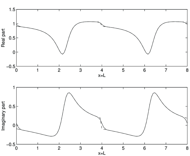
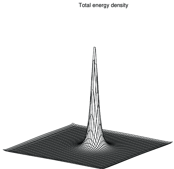
Figure 1: Above: $W_{1}$ (dashed line) and its periodized version $W_{p}$ (solid line) along the line $y=2$ of the fundamental cell. Below: A typical picture for the total energy density associated with $W_{p}$ at $t=0$. The folds at the edges are caused by the periodization procedure.

The upper half of figure (1) illustrates the periodization of $W_{1}$ for a representative line of the fundamental cell. The lower half exhibits the total energy density associated with the periodized field $W_{p}$. It is apparent from this picture that the periodization procedure introduces some perturbation at the borders of the grid in the form of small folds. Under the numerical evolution these perturbations propagate towards the center of the lattice and collapse the lump. In order to minimize such an effect, we improve the initial conditions by ironing out the folds. We do this by implementing a damping function, $\gamma$, that rescales $\partial_{t}\vec{\phi_{p}}\rightarrow\gamma\partial_{t}\vec{\phi_{p}\/},\,\gamma\leq 1.$   The absorbtion is switched off at the time ($t_{0}$) when the folds have disappeared; the resultant configuration serves us as a better, improved set of initial conditions.

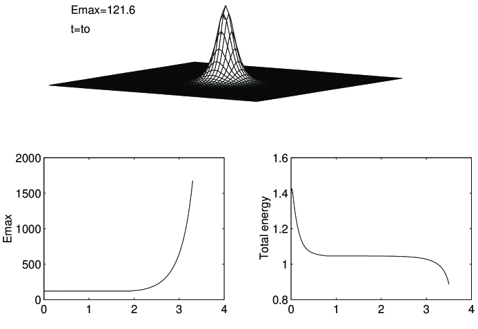
Figure 2: Above: Total energy density at $t_{0}$=0.8, corresponding to our prepared, improved initial one soliton-like configuration. Below: The maximum value of the total energy density ($Emax$) and the total energy vs. $t$. The lump grows infinitely tall soon after $t_{f}\approx$ 3.5, and the numerical procedure collapses.

During the preparatory stage the total energy undergoes a small decrease, in conformity with the absorption that is taking place. Once the latter is turned off, the energy settles near the expected value of one and remains constant until the time ($t_{f}$) when the total energy density becomes so spiky that the numerical procedure breaks down [see figure 2]. Moreover, we have checked that these results do not depend on how the initial conditions were prepared, nor on whether a 9-point or a 13-point laplacian operator was used in the simulations. Having performed many such simulations we are convinced that our results are genuine, i.e., the shrinking is genuine and not a numerical artifact.

4.2 Skyrme case

Next we look at possible ways to stabilizing our solitons. Guided by the experience with the $O(3)$ model in the plane (where the shrinking can be prevented by the addition of two extra terms to the Lagrangian -the Skyrme and the potential term-) we consider the possibility of adding the Skyrme term alone. Adding such a term [13] to the $O(3)$ Lagrangian we have:

$${\cal L}_{skyrme} = \frac{1}{4}(\partial_{\mu}\vec{\phi}).(\partial^{\mu}\vec{\phi})$$ (25)

$$- \frac{\theta_{1}}{4}[(\partial^{\mu}\vec{\phi}.\partial_{\mu}\vec{\phi})^{2}-(\partial^{\mu}\vec{\phi}.\partial^{\nu}\vec{\phi})(\partial_{\mu}\vec{\phi}.\partial_{\nu}\vec{\phi})]$$

or, in the simpler $CP^{1}$ formulation

$${\cal L}_{skyrme}=\frac{|W_{t}|^{2}-2|W_{z}|^{2}}{(1+|W|^{2})^{2}}+8\theta_{1}\frac{|W_{z}|^{2}}{(1+|W|^{2})^{4}}(|W_{t}|^{2}-|W_{z}|^{2}).$$ (26)

The associated static equation of motion reads

$$0=W_{z\bar{z}}-\frac{2\bar{W}W_{z}W_{\bar{z}}}{|W|^{2}+1}$$ (27)

$$+\frac{4\theta_{1}}{(|W|^{2}+1)^{2}}[2\bar{W}_{z\bar{z}}W_{z}W_{\bar{z}}-\bar{W}_{zz}(W_{z})^{2}-\bar{W}_{\bar{z}\bar{z}}(W_{\bar{z}})^{2}+W_{zz}\bar{W}_{z}W_{\bar{z}}$$

$$+W_{\bar{z}\bar{z}}\bar{W}_{\bar{z}}W_{z}-W_{z\bar{z}}(|W_{z}|^{2}+|W_{\bar{z}}|^{2})$$

$$+\frac{2W}{|W|^{2}+1}(|W_{z}|^{2}-|W_{\bar{z}}|^{2})^{2}].$$

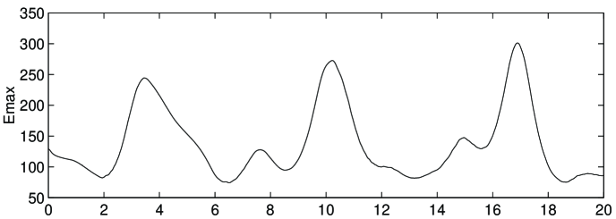
Figure 3: Peak of the total energy density vs. time corresponding to a single-lump in the modified $O(3)$ model with $\theta_{1}=0.001$. The soliton is now stable.

Indeed, we find that thanks to the extra term the energy density of the lump does not increase indefinitely, but instead it oscillates with time in a stable manner. In figure (3) we show the evolution of the amplitude of the total energy density for $\theta_{1}=0.001$. Qualitatively similar pictures are obtained for values of $\theta_{1}$ as small as $\approx$ 0.00015; for smaller values $W_{p}$ is no longer stable.

Note that $W_{p}$ does not exactly satisfy the equation of motion (27), for the term

$$\frac{4\theta_{1}}{(|W|^{2}+1)^{2}}[\bar{W}_{zz}(W_{z})^{2}-2\frac{W|W_{z}|^{4}}{|W|^{2}+1}]$$

does not vanish. Nevertheless, the smallness of $\theta_{1}$ means that our Skyrme model is only a slight perturbation of $O(3)$, and hence $W_{p}$ is a good, if approximate, solution.

Worthy of remark is the fact that (25) does not require a potential-like term to stabilize the lumps. In the $O(3)$ system in the plane with fixed boundary conditions, by contrast, such a term was needed to prevent the solitons from expanding.

5 Solitons of degree 2

5.1 $O(3)$ case

We now move on to the interesting question of collisions, limiting ourselves to two solitons. It is important to bear in mind that the preparatory stage devised for the pathological single-soliton case of section 4 is not required for lumps of degree $\geq 2$. The initial field is given by an order-two fuction of the form (8)-(9):

$$W_{2}=\frac{\sigma(z-a_{1})}{\sigma(z-b_{1})}\frac{\sigma(z-a_{2})}{\sigma(z-b_{2})},\quad a_{1}+a_{2}=b_{1}+b_{2}.$$ (28)

First, consider the situation when the solitons are symmetrically positioned along the horizontal axis and boosted towards each other with relative velocity $v=(0.2,0)$. We select the zeros and poles to be:

$$\left.\begin{array}[]{lll}a_{1}&=&(0.77,1.95),\quad a_{2}=(3.25,1.95);\\ b_{1}&=&(1.32,1.95),\quad b_{2}=(2.70,1.95).\end{array}\right.$$ (29)

The solitons gradually shrink and then undergo a gradual expansion as they approach each other. They collide at the centre of the grid and merge into a complicated ringish structure, where they are no longer distinguishable. After this process the solitons get narrower and narrower as they re-emerge at right angles to the initial direction of motion. Due to their instability, the shrinking process goes on until the solitons get so spiky that the numerical procedure is no longer reliable; this occurs for $t\approx 7$, when max$|\mu|$ as defined in section 3 reaches $\approx$ 10^-4 and higher.

A numerically interesting feature of the periodic $O(3)$ model is that the scattering can also be observed when the solitons are sped ‘away’ from each other, towards the borders of the fundamental cell. This is a good way to test the correctness of our periodic lattice. Applying this to the solitons defined by (29) we also observe the scattering at 90^∘. A representation of this process can be viewed in figure (4).

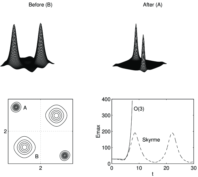
Figure 5: $O(3)$ solitons moving away from the centre along the (0,0)-(4,4) diagonal (B). They collide at the corners and scatter at right angles (A). When the model is supplemented by a Skyrme term the lumps are stable, as shown in the accompanying graph $Emax(t)$.

A typical head-on collision with the solitons initially placed along a diagonal is illustrated in figure (5). The initial position is achieved by the arrangement

$$\left.\begin{array}[]{lll}a_{1}&=&(0.95,0.75),\quad a_{2}=(3.05,3.25);\\ b_{1}&=&(1.22,1.95),\quad b_{2}=(2.78,2.05).\end{array}\right.$$ (30)

After boosting the solitons away from the centre with initial velocity $v=\frac{\sqrt{2}}{10}(1,1)$  -$|v|$=0.2-, the lumps collide at the corner (0,0)=(4,4) and re-appear from (0,4)=(4,0) at right angles to the initial direction of motion. Of course, all four corners are nothing but the same point; there the lumps meet, coalesce and scatter off as already explained. Shortly afterwards, the instability of the system manifests itself in the usual manner, as reflected by the $O(3)$ curve in the graph $Emax(t)$ in figure (5). This diagram also includes the resulting curve of the Skyrme version, as described in subsection (5.2) below. Also, when situated in an arbitrary, non-symmetrical way within the fundamental lattice, the solitons always scatter at ninety degrees when sent head-on against one another (we discuss in more detail this situation in the next section).

We may interpret the instability of (28) under numerical simulations as follows: The solitons start off satisfying the selection rule $a_{1}+a_{2}=b_{1}+b_{2}$, which links them in some manner. Due to inevitable round-off errors during the numerical simulation, the field gets perturbed and so is only approximately described by the original field configuration. As the perturbation is quite small it will excite mainly the degrees of freedom which are zero modes of the original configuration. Thus, in particular, $a_{j}$ and $b_{j}$ will start evolving but in order to remain close to the original configuration they will keep the constraint unbroken. Such evolution may lead to $a_{j}$ and $b{j}$, pairwise, coming close together. This corresponds to the solitons shrinking. To see this note that $|a_{j}-b_{j}|/2$ determines the size of the $j$-th soliton. Note that this shrinking is essentially of the same type as the well known shrinking of any number of solitons on the sphere. We would like to stress that since analytical solutions exist in all topological sectors of index $\geq$ 2, this lack of stability of our two-soliton system is of a different nature than the instability of the single-soliton configuration (and so non-existence of a one-soliton static solution) discussed in the previous section. There the solution does not exist on the lattice or in the continuum; here the solutions do exist in the continuum but are unstable and putting them on the lattice introduces a perturbation which sets off the instability.

5.2 Skyrme case

Let us now consider the Skyrme Lagrangian (26) as applied to two solitons. Head-on collisions along the horizontal axis corresponding to the set up (29) proceed as in the pure $O(3)$ scheme. The Skyrme term, however, prevents the lumps from shrinking indefinitely and renders them stable; their motion can now be followed for as long as desired. For instance, the skyrmions proceed as in figure (4) but, after 90^∘ scattering at the lattice point (0,2)=(4,2), they continue their journey and collide thrice more, reach again their $t$=0 positions and proceed to repeat this cycle anew, as suggested by figure (6). Note the coalescence of the lumps in the corners (subplot $t=11$) which, as mentioned before, are nothing but one and the same point. The plot of the corresponding $Emax(t)$ -not shown- is very much like the one drawn in figure (5) [dashed curve]. All two-skyrmion cases shown in this paper correspond to $\theta_{1}=1/2000$, but the same qualitative behaviour is found for values down to $\approx$ 0.00007. Smaller values cannot prevent the lumps from getting too thin, leading to the breakdown of our code.

An example of solitons located at two arbitrary cell points is given by the parameters

$$\left.\begin{array}[]{lll}a_{1}&=&(0.77,1.30),\quad a_{2}=(3.25,2.70);\\ b_{1}&=&(1.32,1.95),\quad b_{2}=(2.70,2.05).\end{array}\right.$$ (31)

When these solitons are sent to collide head-on, with or without a $\theta_{1}$ term, the scattering, as usual, takes place at $\pi/2$ radians. We shall depict this event within the stable format of the modified model.

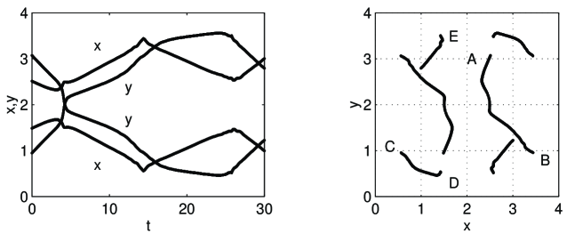
Figure 7: Trajectories of the position of $Emax$ corresponding to the head-on scattering for skyrmions arbitrarily situated in the basic cell. The labels A-E indicate the itinerary of one of the lumps.

Figure (7) refers to two skyrmions directed towards each other with $v=(0.18047,0.0862)$, the speed being 0.2. The coordinates $(x,y)$ correspond to the position of the amplitude $Emax(t)$. The labels A-E are a guide as to the path followed by one of the lumps, the route of the other being given by the corresponding symmetrical points. So a skyrmion-lump starts at $A$ and after $90^{\circ}$ scattering around the centre it continues its itinerary to the position $B$, where it disappears to re-emerge at $C$. Thence the extended structure heads south-east and, having reached point $D$ at $t_{D}\approx$ 14.5, it suddenly changes its path to move south-west (point $E$), unequivocally signalling that a second $90^{\circ}$ scattering has taken place. Regarding the other colliding entity, the one starting at $\approx(1.5,0.9)$, we can see that the said second collision changes the trajectory of this skyrmion from the north-west to the north-east direction. Our numerical simulation terminates at $t_{F}\approx 30$, where $F$ denotes the end of the leg started at $E$.

Note that it is also possible to imagine our solitons as evolving on the surface of a doughnut in ${\cal R}_{3}$, obtained by rotating the circle of radius $r$ and circumference $L$ (the size of the flat manifold $T_{2}$) about a coplanar line ($Z$ axis, say) that does not intersect it. The coordinates $(x\equiv\Upsilon,y\equiv\vartheta)$ serve as the angle of rotation of the plane of the circle and the angle on the circle itself, respectively. The parametric equations of such a torus are the standard

$$X=[R+r\cos(\vartheta)]\cos(\Upsilon),\,Y=[R+r\cos(\vartheta)]\sin(\Upsilon),\,Z=r\sin(\vartheta).$$ (32)

Both the radius $r$ and the distance $R$ from the centre of the circle to the axis of revolution ($Z$) can be calculated from $L$. With the help of (32), the distance $d$ of a lump on the surface of the torus from the origin (0,0,0) may be computed via $d=\sqrt{X^{2}+Y^{2}+Z^{2}}$.

Finally, regarding the situation where the initial velocity of the lumps equals zero, we recall that in the Skyrme model on the sphere the solitons (represented by an approximate field solution) slighty move away from each other, showing the presence of a repulsive force between them [14]. On the other hand, on the torus we have found that our skyrmions, also an approximate solution of the equations of motion, undergo no translation at all as the time elapses. This agrees with our expectations: The net repulsive force on a given lump is now zero due to the presence of similar entities in neighbouring lattices.

6 Concluding remarks

With the help of numerical simulations we have investigated some stability and scattering properties of the non-linear $O(3)$ and Skyrme models with periodic boundary conditions in (2+1) dimensions.

The toroidal $O(3)$ theory has the distinctive feature of possessing analytic soliton solutions only of degree two and higher. This is because the defining fields are elliptic functions. We studied a single-soliton case through a periodic ansatz, which has turned out to be unstable: After some time the lump of energy grows too spiky and the numerical procedure breaks down. Since there are no analytical solutions with topological charge equal to unity, we may regard the above instability as intrinsinc to the model rather than an artifact of our numerical method. However, our ansatz has become stable upon the addition of an extra term (a Skyrme-like term) to the $O(3)$ Lagrangian and, remarkably, under such circumstances our proposed field serves as a good, if approximate, soliton solution of degree one on the torus. Note that unlike the more familiar model on compactified plane, where a second extra term is required to stabilize the solitons, our model necessitates only a Skyrme term to achieve so. In this sense, our model resembles more closely its parent (3+1) dimensional version, where no second extra term is needed, either.

With regards to collisions we have limited ourselves to those involving two solitons (analytic solutions of which do exist on $T_{2}$). Scattering at 90^∘ was observed in all cases considered, both in the pure $O(3)$ and Skyrme schemes. Within the framework of the former the lumps shrink unstably as they evolve, behaviour set off by the perturbation brought about by the discretization procedure. Such instability is of the same type as that exhibited in the familiar $O(3)$ model defined on the compactified plane or topological sphere. As in the one-soliton case, the sole addition of a Skyrme term stabilizes our two-soliton system. Finally, when the skyrmions start off from rest they remain motionless under the numerical simulation, in contrast with the skyrmions on the sphere where they move away from each other due to a repulsive force amongst them.

Acknowledgements

We thank M. Blatter and R. Burkhalter for sending us a subroutine that computes the Weierstrass $\sigma$ function. We are also grateful to B. Piette, J. M. Speight and P. M. Sutcliffe for helpful discussions. RJC is indebted to Universidad del Zulia for their financial support.

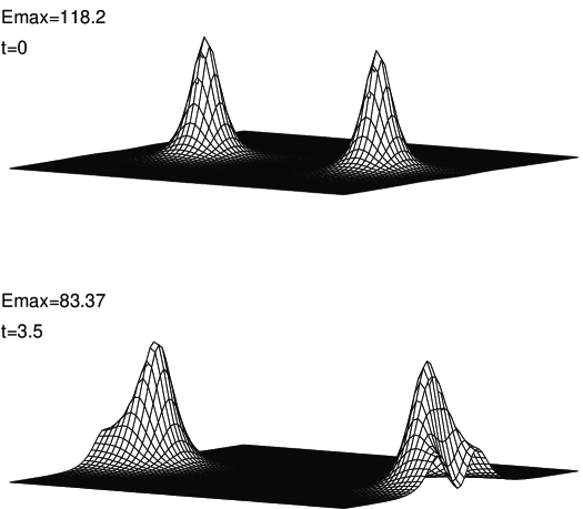
Figure 4: Total energy density corresponding to $O(3)$ solitons moving away from the centre with $v=(0.2,0)$. The amplitude of the lumps gradually decreases as they approach each other, reaching a maximum when they coalesce.

Figure 4 (continued): The solitons scatter at 90^∘. They become very spiky as time progresses but, as shown in figure (6), this is corrected by adding a Skyrme term to the Lagrangian.

Figure 6: Skyrmion scattering ($\theta_{1}$=1/2000) for $v=(0.2,0)$. After scattering like the $O(3)$ solitons of figure 4, the skyrmions do not collapse but go on to collide at $t$=11, 17.5, 25.5 and so forth. At every occasion they scatter at right angles. This cycle repeats itself indefinitely.

References

- [1] Eichenherr H. (1976) Nucl. Phys. B146 215;
- [2] Perelomov A. M. (1981) Physica 4D 1;
- [3] Leese R. A., Peyrard M. and Zakrzewski W. J. (1990) Nonlinearity 3 387;
- [4] Leese R. A., Peyrard M. and Zakrzewski W. J. (1990) Nonlinearity 3 773;
- [5] Zakrzewski W. J. (1991) Nonlinearity 4 429;
- [6] Peyrard M., Piette B. and Zakrzewski W. J. (1992) Nonlinearity 5 563;
- [7] Skyrme T. H. R. (1962) Nucl. Phys. 31 556;
- [8] Erdélyi A. et. al. (1953) Higher transcendental functions vol II Mc Graw Hill pp. 328-337.
- [9] Eells J. and Wood J. C. (1976) Topology 15 263;
- [10] Eells J. and Lemaire L. (1980) Math. Ann. 252 27;
- [11] Richard J. L. and Rouet A. (1987) Nucl. Phys. B211 447;
- [12] Cova R. J. (1995) Helv. Phys. Acta 68 282;
- [13] Azcárraga J. A., Rashid M. S. and Zakrzewski W. J. (1991) Jour. Math. Phys. 32, 1921;
- [14] Cova R. J. and Zakrzewski W. J. (Minsk 1994) Proceedings ‘Quantum Systems’ World Scientific, pp. 84-88.