Graceful exit problem and stress-energy-momentum tensors revisited in the two-dimensional string cosmology

Abstract

We study the graceful exit problem and the role of the stress-energy-momentum tensors in the two-dimensional string cosmology. The one-loop quantum correction of conformal fields is incorporated in the arbitrary large $N$ limit to ensure exact quantum solvability. The only solution which gives the bounded curvature with the asymptotic flatness is restricted to the first branch under some conditions. However, even in this case, the accelerating expansion is forever. We show that the only nonvanishing quantum stress-momentum tensor is the pressure part($T_{xx}$) which is of relevance to the dynamical evolution of the universe in the comoving coordinate. The quantum energy part is zero since the negative contribution of the induced conformal matters always cancels the positive quantity of the induced dilaton part in terms of the constraint equation.

Recently, there has been much interests in the graceful exit problem [1] of the string inflationary cosmology [2] with the scale factor duality [3]. The essential problem is due to the curvature singularity arising from the classical cosmological solutions of low-energy string theory. On the other hand, in the four-dimensional Einstein gravity with the loop effect which is regarded as Einstein frame of string theory [4], some cosmological singularity problems have been studied in terms of the quantum back reaction of space time [5, 6]. Further, the quantum tunneling with the finite probability between the classically distinct phases corresponding to the pre(accelerated) and post(decelerating) big bang can be possible in the low energy string background [7]. This fact may solve the graceful exit problem of the string cosmology.

The exactly soluble Callan-Gidding-Harvey-Strominger(CGHS) model [8, 9], which has been successful to deal with the two-dimensional black holes, has been recently investigated by Rey [10] to show whether or not the branch-changing phase transition appears in the two-dimensional string cosmology. This model was also extended to the generalized two-dimensional dilaton gravity model by Gasperini and Veneziano [11]. The quantum back-reacted solution of the first branch (second branch) with the bounded curvature scalar has been defined within the whole comoving time from the past infinity to the future infinity, so that the second branch (first branch) effectively disappear instead of connecting two distinct branches.

On the other hand, this model has the negative anomaly coefficient which corresponds to the negative Hawking radiation and the number of conformal matter fields are restricted to less than 24. Thus it is natural to study the CGHS model in the manner to take the arbitrary large positive number of matter fields to take good approximation within the one-loop vacuum polarization of the conformal matter fields [13]. Very recently, Bose and Kar [14] suggest the way how to overcome the limit of $N$ by adding a local covariant counter-term and the exact scale factor is obtained.

In this paper, we reconsider the graceful exit problem in the two-dimensional string cosmology with the slightly generalized counter-terms containing the local term of Ref. [14] and mainly study the role of the stress-momentum tensors induced by the quantum corrections. The only solution which gives the bounded curvature with the asymptotic flatness is restricted to the first branch. However, even in this case, the decelerating phase does not appear although the solution has asymptotic flatness. We show that the only nonvanishing quantum stress-energy-momentum tensor is the pressure part($T_{xx}$) which is of relevance to the dynamical evolution of the universe in the comoving coordinate. The total quantum-mechanical energy is zero since the negative contribution of the induced conformal matters always cancels the positive quantity of the induced dilaton part in terms of constraint equation.

Let us now consider the two-dimensional low-energy string theory given by

$$S_{{\rm{DG}}}=\frac{1}{2\pi}\int\/d^{2}x\sqrt{-g}\,e^{-2\phi}\left[R+4(\nabla\phi)^{2}+4\lambda^{2}\right],$$ (1)

where $\phi$ is a dilaton field, and the cosmological constant $\lambda^{2}$ sets to zero in that we are now considering dimensionally reduced low-energy string theory from the critical dimensions. The action for the classical and quantum matter are written in the form of

$$S_{{\rm{Cl}}} = -\frac{1}{2\pi}\int\/d^{2}x\sqrt{-g}\,\frac{1}{2}\sum_{i=1}^{N}(\nabla f_{i})^{2},$$ (2)

$$S_{{\rm{Qt}}} = \frac{\kappa}{2\pi}\int d^{2}x\/\sqrt{-g}\left[-\frac{1}{4}R\frac{1}{\Box}R+q\left(\nabla\phi\right)^{2}-\frac{\gamma}{2}\phi R\right],$$ (3)

where $\kappa=\frac{N-24}{12}$. In Eq. (3), the first term is induced matter part and the second and third represents induced dilaton part. And $q$ and $\gamma$ simply denoted as $(q,\gamma)$ are constants which will be chosen in later for exact solvability. For $(2,6)$, the model was already treated by Bose and Kar in Ref. [14] and for $(0,1)$ it is just the RST model which corresponds to the Rey’s model in the cosmology. For $(1,2)$, it is a black hole model in Ref. [15]. For an arbitrary large $N$ ($N>24$), we assume that the anomaly coefficient $\kappa$ is finite [14]. The nonlocal form of the action (3) is written as by introducing an auxiliary field $\psi$ for later convenience,

$$S_{{\rm{Qt}}}=\frac{\kappa}{2\pi}\int d^{2}x\/\sqrt{-g}\left[\frac{1}{4}R\psi-\frac{1}{16}(\nabla\psi)^{2}+q\left(\nabla\phi\right)^{2}-\frac{\gamma}{2}\phi R\right].$$ (4)

The effective total action is

$$S_{\rm T}=S_{\rm DG}+S_{\rm M},$$ (5)

where the matter part is composed of two pieces of $S_{\rm M}=S_{\rm Cl}+S_{\rm Qt}$. The equations of motion and the constraint equations for this action (5) are

$$G_{\mu\nu}=T_{\mu\nu}^{\rm M}$$ (6)

where

$$G_{\mu\nu}=\frac{2\pi}{\sqrt{-g}}\frac{\delta S_{\rm DG}}{\delta g^{\mu\nu}}$$ (7)

$$\qquad\/=e^{-2\phi}\bigg{[}2\nabla_{\mu}\nabla_{\nu}\phi+2g_{\mu\nu}\left((\nabla\phi)^{2}-\Box\phi\right)\bigg{]},$$ (8)

$$T_{\mu\nu}^{\rm M}\ =-\frac{2\pi}{\sqrt{-g}}\frac{\delta S_{\rm M}}{\delta g^{\mu\nu}}$$ (9)

$$\qquad\,=\frac{1}{2}\sum_{i=1}^{N}\left[\nabla_{\mu}f_{i}\nabla_{\nu}f_{i}-\frac{1}{2}(\nabla f_{i})^{2}\right]+\frac{\kappa}{4}\left[\nabla_{\mu}\nabla_{\nu}\psi+\frac{1}{4}\nabla_{\mu}\psi\nabla_{\nu}\psi-g_{\mu\nu}\left(\Box\psi+\frac{1}{8}(\nabla\psi)^{2}\right)\right]$$ (10)

$$\qquad\ \ \ -\frac{\gamma\kappa}{2}\bigg{[}\nabla_{\mu}\nabla_{\nu}\phi-g_{\mu\nu}\Box\phi\bigg{]}-q\kappa\left[\nabla_{\mu}\phi\nabla_{\nu}\phi-\frac{1}{2}g_{\mu\nu}(\nabla\phi)^{2}\right],$$ (11)

and the other equations of motion for $\phi$, $f_{i}$, and $\psi$ are given by

$$e^{-2\phi}\left[R+4\Box\phi-4(\nabla\phi)^{2}\right]=-\frac{\gamma\kappa}{4}R-q\kappa\Box\phi,$$ (12)

$$\Box f_{i}=0,$$ (13)

$$\Box\psi=-2R.$$ (14)

In the conformal gauge, $g_{\pm\mp}=-\frac{1}{2}e^{2\rho}$, $g_{\pm\pm}=0$, the total action and the constraints are given by

$$S_{\rm T} = \frac{1}{\pi}\int\/d^{2}x\bigg{\{}e^{-2\phi}\left[2\partial_{+}\partial_{-}\rho-4\partial_{+}\phi\partial_{-}\phi\right]-\kappa\Big{[}\partial_{+}\rho\partial_{-}\rho+\gamma\phi\partial_{+}\partial_{-}\rho$$ (16)

$$+q\partial_{+}\phi\partial_{-}\phi\Big{]}+\frac{1}{2}\sum_{i}\partial_{+}f_{i}\partial_{-}f_{i}\bigg{\}}$$

and

$$e^{-2\phi}\left[4\partial_{\pm}\rho\partial_{\pm}\phi-2\partial_{\pm}^{2}\phi\right]+\frac{1}{2}\sum_{i=1}^{N}\left(\partial_{\pm}f\right)^{2}+\kappa\left[\partial_{\pm}^{2}\rho-\left(\partial_{\pm}\rho\right)^{2}\right]$$ (17)

$$\qquad\qquad\qquad\qquad\qquad-\frac{\gamma\kappa}{2}\left(\partial_{\pm}^{2}\phi-2\partial_{\pm}\rho\partial_{\pm}\phi\right)-q\kappa\left(\partial_{\pm}\phi\right)^{2}-\kappa t_{\pm}=0,$$ (18)

where $t_{\pm}$ reflects the nonlocality of the induced gravity of the conformal anomaly [16]and we set $q=\gamma-1$ to make the equations exactly solvable. Without the classical matter, $f_{i}=0$, defining new fields as follows [16, 17, 18],

$$\Omega = -\frac{\kappa}{2}(\gamma-2)\phi+e^{-2\phi},$$ (19)

$$\chi = \kappa\rho-\frac{\gamma\kappa}{2}\phi+e^{-2\phi},$$ (20)

the gauge fixed action is obtained in the simple form of

$$S_{\rm T}=\frac{1}{\pi}\int\/d^{2}x\left[\frac{1}{\kappa}\partial_{+}\Omega\partial_{-}\Omega-\frac{1}{\kappa}\partial_{+}\chi\partial_{-}\chi+\frac{1}{2}\sum_{i=1}^{N}\partial_{+}f_{i}\partial_{-}f_{i}\right]$$ (21)

and the equations of motion and the constraints are given by

$$\partial_{+}\partial_{-}\Omega=\partial_{+}\partial_{-}\chi=0,$$ (22)

$$G_{\pm\pm}-T_{\pm\pm}^{\rm M} = -\frac{1}{\kappa}\left(\partial_{\pm}\Omega\right)^{2}+\frac{1}{\kappa}\left(\partial_{\pm}\chi\right)^{2}-\partial_{\pm}^{2}\chi-\frac{1}{2}\sum_{i=1}^{N}(\nabla f_{i})^{2}+\kappa t_{\pm}$$ (23)

$$= 0.$$ (24)

In the homogeneous condition of fields, we obtain equations of motion in the simple forms of

$$\ddot{\chi}(t)=\ddot{\Omega}(t)=0,$$ (25)

and they yield solutions,

$$\chi = \kappa\rho-\frac{\gamma\kappa}{2}\phi+e^{-2\phi}=\chi_{0}t+A,$$ (26)

$$\Omega = \frac{\kappa}{2}\left(2-\gamma\right)\phi+e^{-2\phi}=\Omega_{0}t+B,$$ (27)

where $\chi_{0},~{}~{}\Omega_{0},~{}~{}A,$ and $B$ are constants. The constraint (24) becomes, by using the solutions (26) and (27),

$$\kappa t_{\pm}-\frac{1}{4\kappa}\left(\Omega_{0}-\chi_{0}\right)\left(\Omega_{0}+\chi_{0}\right)=0.$$ (28)

Choosing the quantum matter state as vacuum, $t_{\pm}=0$, the first branch which corresponds to the case with $\Omega_{0}=\chi_{0}\equiv-M(<0)$ and $A=B=0$ is obtained [10].

At this juncture, let us study the boundedness of the scalar curvature which is given by

$$R = 2e^{-2\rho}\ddot{\rho}(t)$$ (29)

$$= M^{2}e^{-2\rho}e^{-2\phi}\left[e^{-2\phi}+\frac{\kappa}{4}(\gamma-2)\right]^{-3},$$ (30)

in terms of the explicit solutions (26) and (27). It is natural to confine the constant as $\gamma>2$ to avoid the singularity of the curvature. If $\gamma<2$, $\kappa$ should be negative [12]. The solution (26) and (27) belongs to the two branches depending on the parameters. Note that as far as we are concerned with the first branch solution, the accelerating expansion is only possible since without any assumption, the curvature is positive definite $\ddot{a}>0$ in the whole range of the conformal time (or comoving time) in our case. In fact, even for the negative $\kappa$ which corresponds to Rey’s model, there is no decelerating phase [12].

On the other hand, we are concerned with the stress-energy-momentum tensors obtained from (11),

$$T_{\pm\pm}^{\rm M} = \kappa\left[\partial_{\pm}^{2}\rho-(\partial_{\pm}\rho)^{2}-t_{\pm}(x^{\pm})\right]-\frac{\gamma\kappa}{2}\left[\partial_{\pm}^{2}\phi-2\partial_{\pm}\rho\partial_{\pm}\phi\right]-\kappa(\gamma-1)(\partial_{\pm}\phi)^{2},$$ (31)

$$T_{+-}^{\rm M} = -\kappa\partial_{+}\partial_{-}\rho+\frac{\gamma\kappa}{2}\partial_{+}\partial_{-}\phi.$$ (32)

By using the relation, $\rho(t)=\ln a(\tau)$ with $dt=d\tau/a(\tau)$, one can perform the coordinate transformation to the comoving time, and then Eqs. (31) and (32) are

$$T_{\tau\tau}^{\rm M}(\tau) = 0,$$ (33)

$$T_{\tau x}^{\rm M}(\tau) = 0,$$ (34)

$$T_{xx}^{\rm M}(\tau) = -\frac{2M^{2}\left[M\tau+\sqrt{(M\tau)^{2}+4\kappa(\gamma-2)}~{}\right]}{\left[(M\tau)^{2}+4\kappa(\gamma-2)\right]^{\frac{3}{2}}}.$$ (35)

Note that the energy $T_{\tau\tau}^{\rm M}$ and the momentum $T_{\tau x}^{\rm M}$ vanish and $T_{xx}^{\rm M}$ has a negative definite. As a result, the induced energy-momentum tensors are zero at anytime while the stress part which corresponds to the pressure of the prefect fluid has a time-dependent negative value. This fact seems to be unusual and we clarify in detail in the followings.

From now on, we choose comoving coordinates on the purpose of directly computing the stress-energy-momentum tensors instead of transforming from the results in the conformal gauge to the comoving coordinates. The energy-momentum tensors are not true tensor generically in the general coordinate transformation, for example, for the conformal transformation in the black hole geometry [16]. So we now calculate the expectation value of the stress-energy-momentum tensors from the beginning in the comoving coordinates given by

$$ds^{2}=-d\tau^{2}+a^{2}(\tau)dx^{2}.$$ (36)

Then the classical dilaton gravity part $G_{\mu\nu}$ is written as

$$G_{\tau\tau}(\tau)=2e^{-2\phi}\left[\dot{\phi}^{2}-\frac{\dot{a}}{a}\dot{\phi}\right],$$ (37)

$$G_{\tau x}(\tau)=0,$$ (38)

$$G_{xx}(\tau)=2a^{2}e^{-2\phi}\left[\ddot{\phi}-\dot{\phi}^{2}\right],$$ (39)

and the stress-energy-momentum tensors are, respectively,

$$T_{\tau\tau}^{\rm M}(\tau)=\frac{1}{4}\sum_{i=1}^{N}\dot{f}_{i}^{2}-\frac{\kappa}{2}\left(\frac{\dot{a}}{a}\right)^{2}+\frac{\gamma\kappa}{2}\frac{\dot{a}}{a}\dot{\phi}-\frac{1}{2}q\kappa\dot{\phi}^{2}-\kappa t_{\tau\tau},$$ (40)

$$T_{\tau x}^{\rm M}(\tau)=0,$$ (41)

$$T_{xx}^{\rm M}(\tau)=a^{2}\left\{\frac{1}{4}\sum_{i=1}^{N}\dot{f}_{i}^{2}+\kappa\left[\frac{\ddot{a}}{a}-\frac{1}{2}\left(\frac{\dot{a}}{a}\right)^{2}\right]-\frac{\gamma\kappa}{2}\ddot{\phi}-\frac{1}{2}q\kappa\dot{\phi}^{2}\right\}-\kappa t_{xx},$$ (42)

where the overdots denote the differentiation with respect to the comoving time $\tau$. The Eqs. (12), (13), and (14) are written in the form of

$$e^{-2\phi}\left(\frac{2\ddot{a}}{a}+4\dot{\phi}^{2}-4\ddot{\phi}-4\frac{\dot{a}}{a}\dot{\phi}\right)=-\frac{\gamma\kappa}{2}\frac{\ddot{a}}{a}+q\kappa\left(\ddot{\phi}+\frac{\dot{a}}{a}\dot{\phi}\right),$$ (43)

$$\ddot{f}_{i}+\frac{\dot{a}}{a}\dot{f}_{i}=0,$$ (44)

$$\ddot{\psi}+\frac{\dot{a}}{a}\dot{\psi}=4\frac{\ddot{a}}{a}.$$ (45)

By eliminating the auxiliary field $\dot{\psi}$, the integration ambiguities $t_{\tau\tau}(\tau)$ and $t_{xx}(\tau)$ were obtained as $a^{2}\kappa t_{\tau\tau}=\kappa t_{xx}=-\frac{\kappa}{32}C^{2}$, where C is an arbitrary constant. Thus $t_{\tau\tau}$ and $t_{xx}$ reflect the nonlocality of the effective action. To find an exact solution, we set $f_{i}=0$, $q=\gamma-1$, and $C=0$. The constraint equation $G_{\tau\tau}-T_{\tau\tau}^{\rm M}=0$ from Eqs. (37) and (40) is neatly expressed as

$$G_{\tau\tau}-T_{\tau\tau}^{\rm M} = -(\dot{\phi}-\frac{\dot{a}}{a})\left[-2\dot{\phi}e^{-2\phi}+\kappa\left(\frac{1+\gamma}{2}\dot{\phi}+\frac{1}{2}\frac{\dot{a}}{a}\right)\right]$$ (46)

$$= 0,$$ (47)

and we choose $\dot{\phi}=\frac{\dot{a}}{a}$, corresponding to the first branch in Ref. [10, 14]. Then note that $T_{\tau\tau}^{\rm{M}}(\tau)$ is zero as far as we are concerned with the first branch, which is easily shown by Eq. (40). On the other hand, the dynamical equation of motion from Eqs. (39) and (42) is

$$G_{xx}-T_{xx}^{\rm M}=0,$$ (48)

which yields

$$\frac{\kappa}{2}\left(\frac{\gamma}{2}-1\right)a(\tau)-\frac{1}{a(\tau)}=\alpha\tau+\beta,$$ (49)

where $G_{xx}=2\left[\frac{\ddot{a}}{a}-2\left(\frac{\dot{a}}{a}\right)^{2}\right]$ and $T_{xx}^{\rm M}=-\frac{\kappa}{2}(\gamma-2)a\ddot{a}$ in terms of scalar factor. Note that if $\alpha$ is fixed as $\frac{1}{2}M$ and the integration constant $\beta$ is zero, then $T_{\tau\tau}^{\rm M}(\tau)$ and $T_{xx}^{\rm M}(\tau)$ are exactly given by Eqs. (33) and (35). From the above solution (49), the scale factor and the curvature are given by

$$a(\tau) = \frac{2}{\kappa(\gamma-2)}\left\{\alpha\tau+\sqrt{(\alpha\tau)^{2}+\kappa(\gamma-2)}\right\},$$ (50)

$$R(\tau) = \frac{2\kappa(\gamma-2)\alpha^{2}}{\left[\alpha^{2}\tau^{2}+\kappa(\gamma-2)\right]^{\frac{3}{2}}\left[\alpha\tau+\sqrt{(\alpha\tau)^{2}+\kappa(\gamma-2)}\right]},$$ (51)

where these are essentially same with those of Bose and Kar in Ref. [14]. In fact, the energy-momentum tensors $T_{\pm\pm}^{{\rm M}}$ (or $T_{\tau\tau}^{{\rm M}}$) are composed of the induced conformal matter density and the dilaton part, however, they are exactly canceled, which is shown by direct calculation of Eq. (40). So, Eqs. (33), (34), and (35) are exactly reproduced from Eqs. (40), (41),and (42) without considering an anomalous transformation. Therefore, the dynamical evolution of the back-reacted geometry in this cosmology is due to the quantum-mechanically induced shear from Eq. (48). Our energy density is parted as a matter of convenience in two contributions from the nonlocal effective action and some local ambiguity parts. In fact, the split of energy momentum density is arbitrary so that the total energy momentum density is in fact meaningful. And this null value can be changed by the addition of the classical energy of the conformal fields or choosing the different boundary condition $t_{\pm}$.

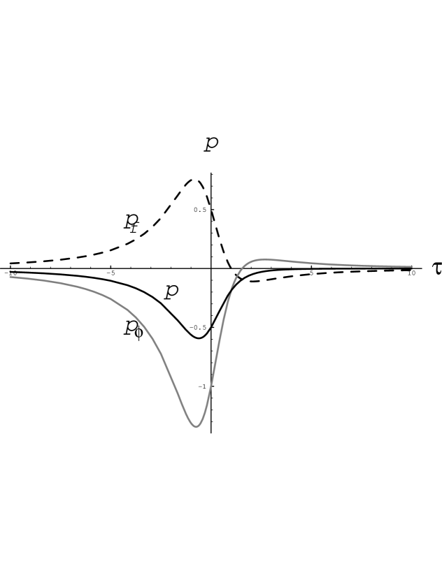
FIG. 1.: $p_{f}$ and $p_{\phi}$ have not definite sign, however the total pressure $p$ is negative definite.

As a comment, it is easily shown that for $\tau\rightarrow-\infty$, $a(\tau)\rightarrow-\frac{1}{\alpha\tau}$ and $R\rightarrow\left(\frac{2}{-\tau}\right)^{2}$ (superinflation phase). In the limit of far future, $\tau\rightarrow+\infty$, $a(\tau)\sim\alpha\tau$ and $R\sim\frac{1}{(\tau)^{2}}$ which corresponds to the Milne universe (flat space-time). In the above analysis, the universe keeps on accelerating expansion since $\dot{a}(\tau)>0$ and $\ddot{a}(\tau)>0$ with the bounded curvature. The expected decelerating phase [7] in the string cosmology does not appear even in the Rey’s model [10].

If we assume the induced quantum matter as a perfect fluid, then the stress-energy-momentum tensors are

$$T_{\mu\nu}^{\rm M}=pg_{\mu\nu}+(p+\rho)u_{\mu}u_{\nu},$$ (52)

where $u_{\mu}=(1,0)$, and $p$ and $\rho$ are pressure and energy density, respectively. Then the only nonvanishing tensor is the shear part and is written in the form of

$$p = \frac{1}{a^{2}}T_{xx}^{\rm M},$$ (53)

$$= -\frac{\alpha^{2}\kappa^{2}(\gamma-2)^{2}}{2\left[(\alpha\tau)^{2}+\kappa(\gamma-2)\right]^{\frac{3}{2}}\left[\alpha\tau+\sqrt{(\alpha\tau)^{2}+\kappa(\gamma-2)}\right]}.$$ (54)

The matter and dilaton contribution to the pressure can be worked out separately, and then they have not definite sign (see Fig.1). The pressure $p_{f}$ from the induced matter and $p_{\phi}$ from the induced dilaton part in Eq. (11) are explicitly given by

$$p_{f} = \kappa\alpha^{2}\left[(\alpha\tau)^{2}+\kappa(\gamma-2)\right]^{-\frac{3}{2}}\left[-\alpha\tau+\frac{1}{2}\sqrt{(\alpha\tau)^{2}+\kappa(\gamma-2)}\right],$$ (55)

$$p_{\phi} = \kappa\alpha^{2}\left[(\alpha\tau)^{2}+\kappa(\gamma-2)\right]^{-\frac{3}{2}}\left[\frac{\gamma}{2}\alpha\tau+\frac{1-\gamma}{2}\sqrt{(\alpha\tau)^{2}+\kappa(\gamma-2)}\right].$$ (56)

However, the total pressure is always negative definite and depends on time. Hence one can state even though there is no total energy density as a source, the pressure of the radiation fields (shear) by the quantum effect appears to make the curvature finite.

Now, it seems to be appropriate to discuss the positivity of $\kappa$. It might be possible formally to take the negative limit $N\rightarrow-\infty$ to obtain the good approximation if one restricts $N<24$ like in Ref. [10]. However, there may be some reasons why we have taken the physical condition $N>24$ or $\kappa>0$. Essentially it arises from the conformal field theory and consistency condition of locally symmetric theory. First, from the conformal field theory point of view, the central charge of matter field $c_{matter}=N$ should be positive definite for the unitary theory. In other words, in a nonunitary theory, the central charge is negative. So the number $N$ should be positive definite. As a second step, the gravitational field turn on, the total central charge in our case is shifted by $c_{total}=c_{matter}+c_{ghost}+c_{gravity}=N-26+1+1-12\kappa=N-24-12\kappa$. Up to this stage, $\kappa$ is still arbitrary. The total central charge should be zero in order to preserve the consistency of the theory, then $\kappa=\frac{N-24}{12}$. So the large $\kappa$ or $N$ limit can be possible when $N>24$ as far as we take $N>0$. On the other hand, the restriction of $N>24$ in our theory from the regularity of curvature scalar also seems to be also awkward. This can be improved by adding the Strominger’s ghost decoupling term [19] to the quantum effective action by using the regularization ambiguity, then $\kappa=\frac{N}{12}$ is obtained. Therefore, neither $N>24$ or $N<24$ may be necessary.

Two final remarks are in order. First, we did not consider the anomalous transformation or Schwartzian derivative between the two coordinates (conformal and comoving coordinates). As easily seen from the results in the above two coordinates, there is no anomalous transformation of stress-energy-momentum tensors in our cosmological model. So the stress-energy-momentum tensors in the conformal gauge was transformed to the comoving coordinate without any anomaly and result in the vanishing energy-momentum tensors. This result is compatible with the direct calculations in the comoving coordinate. So the integration ambiguity $t_{\pm\pm}(t)=0$ was maintained in the form $t_{\tau\tau}(\tau)=t_{xx}(\tau)=0$. In the black hole case, the anomalous transformation of stress-energy-momentum tensors was assumed to be canceled by the anomalous transformation of the integration ambiguity, $t_{\pm\pm}(x^{+},x^{-})$. Secondly, the covariant conservation of $T_{\mu\nu}^{M}$ is spoiled by the local counter term. In fact, since we are in the string-frame, the classical dilaton gravity part is not purely geometrical on the contrary to the Einstein gravity in the four dimensions. So there does not exist the covariant conservation of the matter part although the whole tensor $G_{\mu\nu}-T_{\mu\nu}^{\rm M}=0$ is covariant. To make this explicit, by using the Eqs. (31) and (32), one obtains $\nabla_{\mu}T^{\mu\pm}_{\rm M}=4\kappa(\gamma-2q)e^{-4\phi}\partial_{\mp}\phi\partial_{\pm}\partial_{\mp}\phi$. Therefore, the stress-energy-momentum tensor of induced quantum matter is not covariantly conserved unless $\gamma=2q$. On the other hand, we assumed $q=\gamma-1$ for exact solvability. So the covariant conservation of matter part and exact solubility of the closed form require $(1,2)$ called BPP model [15], however, the curvature scalar is not bounded.

In summary, we have studied the superinflation of pre-big bang phase is smoothly connected to flat universe in the large $N$ limit in the CGHS model. As far as we are concerned with the vacuum theory, there is neither energy nor momentum while the pressure (shear) of the radiation field governs the universe in terms of the quantum back reaction in this model.

Acknowledgments

This work was supported by Ministry of Education, 1997, Project No. BSRI-97-2414, and Korea Science and Engineering Foundation through the Center for Theoretical Physics in Seoul National University(1997).

REFERENCES

[1] R. Brustein and G. Veneziano, Phys. Lett. B329
(1994) 429; N. Kaloper, R. Madden, and K. A. Olive, Nucl. Phys.
B452 (1995) 677; R. Easther, K. Maeda, and D. Wands,
Phys. Rev. D53 (1996) 4247.
[2] M. Gasperini and G. Veneziano, Astropart. Phys. 1
(1993) 317; Mod. Phys. Lett. A8 (1993) 3701;
Phys. Rev. D50 (1994) 2519.
[3] G. Veneziano, Phys. Lett. B265 (1991) 287; A. Sen,
Phys. Lett. B271 (1991) 295; A. Tseytlin, Mod.
Phys. Lett. A6 (1991) 1721.
[4] M. Gasperini and G. Veneziano, Mod. Phys. Lett. A8 (1993)
3701.
[5] I. Antoniadis, J. Rizos, and K. Tamvakis, Nucl. Phys. B415
(1994) 497.
[6] R. Easther and K. Maeda, Phys. Rev. D54 (1996) 7252.
[7] M. Gasperini, J. Maharana, and G. Veneziano, Nucl. Phys.
B472 (1996) 349.
[8] C. G. Callan, S. B. Giddings, J. A. Harvey, and A. Strominger,
Phys. Rev. D45 (1992) R1005.
[9] J. G. Russo, L. Susskind, and L. Thorlacius, Phys. Rev.
D46 (1992) 3444; Phys. Rev. D47 (1993) 533.
[10] S.-J. Rey, Phys. Rev. Lett. 77 (1996) 1929.
[11] M. Gasperini and G. Veneziano, Phys. Lett. B387
(1996) 715.
[12] W.T. Kim and M. Yoon, Quantization of dilaton cosmology in
two dimensions, hep-th/9704115.
[13] S. Bose, Solving the graceful exit problem in superstring
cosmology, hep-th/9704175.
[14] S. Bose and S. Kar, Exact solutions in
two-dimensional string cosmology with back reaction, hep-th/9705061.
[15] S. K. Bose, L. Parker, and Y. Peleg, Phys. Rev. Lett.
76 (1996) 861.
[16] W. T. Kim and J. Lee, Phys. Rev. D 52 (1995) 2232.
[17] A. Bilal and C. Callan, Nucl. Phys. B394 (1993) 73.