Preprint:THU-97/13

hep-th/9706021

June 1997

Explicit solutions for Point Particles and Black Holes
in spaces of constant curvature in 2+1-D Gravity
M.Welling

Instituut voor Theoretische Fysica
Rijksuniversiteit Utrecht
Princetonplein 5
P.O. Box 80006
3508 TA Utrecht
The Netherlands

In this paper we consider space-times containing matter expanding or contracting according to a time-dependent scale factor. Cosmologies with vanishing, positive or negative cosmological constant are considered. In the case of vanishing or negative cosmological constant open and closed spatial surfaces are solutions while in the case of positive cosmological constant only closed surfaces exist. The gravitational field is solved explicitly in the case of 1 or 2 particles, 1 black-hole, and 1 black-hole vacuum state.

PACS numbers: 0460K, 0420J

1 Introduction

Shortly after the discovery of explicit solutions for gravitating point particles in 2+1 dimensions [2], Deser and Jackiw studied point particles in de Sitter (dS) space-time [3]. They found static solutions where two particles are located at the north and south pole of a sphere. Their effect on the vacuum solution is to cut out a wedgelike region between two circles emanating from particle 1 and ending at particle 2. The width of the wedge is proportional to the particle’s mass.

Later Banãdos, Teitelboim and Zanelli discovered the possibility of a black hole in anti de Sitter (AdS) space-time [10]. Subsequent publications were concerned with the possibility of multi-particle or multi-black hole states [11, 12, 13]. The fact that these multi-object states can be fully understood is due to the fact that no local degrees of freedom exist in 2+1-D gravity: all interactions are topological. This fact was used by us [7] and Ciafaloni et. al. [8] to write down explicit solutions for multi-particle states in ’ordinary 2+1 gravity’ ($\Lambda=0$). In this paper we are concerned with a special class of solutions in 2+1 D cosmological gravity, namely the ones in which all matter expands or contracts with the same scale factor. It is typical for gravity in 2+1 dimensions that the expansion rate is not influenced by the amount of matter we add to our space-time. So the scale factor depends on $\Lambda$ and time, but not on the matter distribution. The geometry of the spatial slice is described by the Liouville equation (with a different sign for dS and AdS space-time). The solution to this equation is known in terms of an arbitrary analytic function $f(z)$. If we add matter to space-time this mapping function becomes multivalued. For a black hole (BH) we find hyperbolic monodromy, for a black hole vacuum (BHV) we find parabolic monodromy and for a particle we find elliptic monodromy. In fact the matter is completely described by these monodromy transormations (or multivaluedness) of the function $f(z)$. We were able to find explicit solutions for this function in the case of 1 and 2 particles, of a BH and of a BHV. The problem of finding multi-particle or multi-BH solutions is equivalent to a Riemann-Hilbert problem with all three types of monodromy. For vanishing and negative cosmological constant these solutions were considered on spatially open universes. The question which matter distributions form spatially closed solutions, is answered by the uniformization theorem.

2 Spaces of constant negative Curvature

In this section we will describe two space-times that have constant negative curvature. The simplest example one can think of is to slice ordinary Minkowski space-time into time surfaces with constant negative curvature:

$$X = t\sinh\theta\cos\varphi$$ (1)

$$Y = t\sinh\theta\sin\varphi$$ (2)

$$T = t\cosh\theta$$ (3)

The Minkowski line element in these coordinates is:

$$ds^{2}=-dt^{2}+t^{2}(d\theta^{2}+\sinh^{2}\theta d\varphi^{2})$$ (4)

The intrinsic curvature of the two dimensional $t=$constant surface is now:

$${}^{(2)}R=-\frac{2}{t^{2}}$$ (5)

According to the (contracted) Gauss-Codazzi equations it should be compensated by the extrinsic curvature $K_{ij}$ as follows:

$${}^{(2)}R-K_{ij}K^{ij}+K^{2}=0$$ (6)

where $K$ is defined as the trace of $K_{ij}$. In the above case we have:

$$K_{ij}=\frac{1}{2}Kg_{ij}~{}~{}~{}~{}~{}~{}~{}~{}K=\frac{-1}{\sqrt{g}}\frac{d}{dt}\sqrt{g}=\frac{-2}{t}$$ (7)

It is important to recognize that we insist on using Gaussian comoving coordinates defined by:

$$g_{00}=-1~{}~{}~{}~{}~{}~{}g_{0i}=0$$ (8)

As it turns out it will be convenient to use complex coordinates in the following:

$$z=\tanh(\frac{\theta}{2})e^{i\varphi}~{}~{}~{}~{}~{}~{}\bar{z}=\tanh(\frac{\theta}{2})e^{-i\varphi}$$ (9)

The line element becomes:

$$ds^{2}=-dt^{2}+\frac{4S^{2}(t)}{(1-z\bar{z})^{2}}dz~{}d\bar{z}~{}~{}~{}~{}~{}~{}S(t)=t$$ (10)

The spatial part is of course precisely the metric on a Poincaré disc, with a scale $S(t)$ depending on time. Up to this point we did nothing but trivial coordinate transformations. Notice that this metric is invariant under the following SU(1,1) transformations:

$$z\rightarrow\frac{\alpha z+\beta}{\bar{\beta}z+\bar{\alpha}}~{}~{}~{}~{}~{}~{}~{}~{}~{}~{}\alpha,\beta\in~{}C$$ (11)

Our next example is Anti-de Sitter space (AdS). In this case we have to include a negative cosmological constant into Einsteins equations. It is most convenient to embed this space into a four dimensional space-time with two negative and two positive signs:

$$ds^{2}=-dU^{2}-dV^{2}+dX^{2}+dY^{2}$$ (12)

The constraint determining AdS space-time is given by:

$$-U^{2}-V^{2}+X^{2}+Y^{2}=-\ell^{2}~{}~{}~{}~{}~{}~{}\Lambda=-\frac{1}{\ell^{2}}$$ (13)

Both the line element and the constraint are invariant under SO(2,2) transformations which is the symmetry group of AdS space-time. Because it has the same dimensionality as the Poincaré group, AdS space is also maximally symmetric. The explicit embedding is given by:

$$X = \ell\cos\tau\sinh\theta\cos\varphi$$ (14)

$$Y = \ell\cos\tau\sinh\theta\sin\varphi$$ (15)

$$U = \ell\cos\tau\cosh\theta$$ (16)

$$V = \ell\sin\tau$$ (17)

From this embedding we can see that every instant of time AdS space is a hyperbole with ‘radius’ $\ell\cos\tau$. For $\tau\in(-\frac{1}{2}\pi,0)$ this hyperbole is contracting, at $\tau=0$ it is momentarily static and for $\tau\in(0,\frac{1}{2}\pi)$ it is expanding. Actually, AdS is the universal covering of this space by unwinding the time coordinate. The line element is:

$$ds^{2}=\ell^{2}\{-d\tau^{2}+\cos^{2}\tau(d\theta^{2}+\sinh^{2}\theta d\varphi^{2})\}$$ (18)

One immediately recognizes the similarity with (4). Going to complex coordinates (9) and defining a dimensionful time: $t=\ell\tau$, gives again the line element (10) but with a different scale factor:

$$S(t)=\ell\cos\frac{t}{\ell}$$ (19)

The intrinsic two dimensional curvature is given by:

$${}^{(2)}R=\frac{-2}{S^{2}}=\frac{-2}{\ell^{2}\cos^{2}\frac{t}{\ell}}$$ (20)

The Gauss-Codazzi equation now also involves the cosmological constant:

$${}^{(2)}R-K_{ij}K^{ij}+K^{2}+\frac{2}{\ell^{2}}=0$$ (21)

with

$$K=\frac{2}{\ell}\tan\frac{t}{\ell}$$ (22)

Notice that at $t=\pm\frac{1}{2}\pi\ell$ both intrinsic and extrinsic curvature diverge [12]. Notice also that at $t=0$ we have $K=0$. This implies that at $t=0$ the space-time is momentarily static (or time symmetric)[11].

3 Inclusion of Point Particles

In section 1 we studied two vacuum solutions to Einstein’s equations with and without cosmological constant. In this section we will invert the line of reasoning and assume a metric of the following form:

$$ds^{2}=-dt^{2}+S^{2}(t)e^{\phi(z,\bar{z})}dzd\bar{z}$$ (23)

and solve for $S(t)$ and $e^{\phi}$. Notice that we choose Gauss normal coordinates (i.e. $g_{00}=-1$ and $g_{0i}=0$). Furthermore we assume that the gravitational field looks isotropic everywhere. The vacuum solutions of section 1 are found if we set:

$$e^{\phi}=\frac{4}{(1-z\bar{z})^{2}}$$ (24)

In the following we will explicitly solve the Einstein equations and find out whether there is some freedom left to introduce point masses. The Einstein tensor $G_{\mu}^{\nu}$ in Gaussian normal coordinates was calculated by Sachs in [14]. With the extra condition of isotropy we find:

$$G_{i}^{0} = 0$$ (25)

$$G_{0}^{0} = -\frac{1}{2}(^{(2)}R+\frac{1}{2}K^{2})$$ (26)

$$G_{i}^{j} = \frac{1}{2}\dot{K}\delta_{i}^{j}-\frac{1}{4}K^{2}\delta_{i}^{j}$$ (27)

with:

$${}^{(2)}R = -\frac{e^{-\phi}}{S^{2}}\partial^{i}\partial_{i}\phi$$ (28)

$$K = -2\frac{\dot{S}}{S}$$ (29)

The Einstein equations with cosmological constant are:

$$G_{\mu}^{\nu}+\frac{\delta_{\mu}^{\nu}}{\ell^{2}}=8\pi GT_{\mu}^{\nu}$$ (30)

Combining the above formula’s we can deduce two relevant equations:

$$\partial\bar{\partial}\phi-\frac{1}{2}(\dot{S}^{2}+\frac{S^{2}}{\ell^{2}})e^{\phi}=-4\pi GS^{2}e^{\phi}T^{00}$$ (31)

$$\ddot{S}+\frac{S}{\ell^{2}}=0$$ (32)

where $\partial\equiv\frac{\partial}{\partial z}$, $\bar{\partial}\equiv\frac{\partial}{\partial\bar{z}}$ and $z=x+iy$. As we are interested in point sources at fixed coordinates $z_{n}$, we use the following Ansatz for the energy momentum tensor:

$$T^{ij}=T^{0i} = 0$$ (33)

$$\sqrt{{}^{(2)}g}T^{00} = S^{2}e^{\phi}T^{00}=\sum_{n}\alpha_{n}\delta^{2}(z-z_{n})$$ (34)

where $\alpha_{n}$ are constants to be determined later. The next step is to solve equation (32). In the case where $\Lambda=0$ (or $\ell=\infty$) we find:

$$S(t)=At+B$$ (35)

If the ‘big bang’ takes place at $t=0$ we must set $B=0$. For simplicity we will normalize the ‘scaling-velocity’ $A=1$. In the case of a non vanishing cosmological constant we impose the condition that at $t=0$ the solution is time symmetric: $\dot{S}=0$. The solution is in that case:

$$S(t)=A\ell\cos(\frac{t}{\ell})$$ (36)

In the following we will also set $A=1$ for simplicity. Substituting these solutions into equation (31) we find in both cases:

$$\partial\bar{\partial}\phi-\frac{1}{2}e^{\phi}=-4\pi G\sum_{n}\alpha_{n}\delta^{2}(z-z_{n})$$ (37)

This equation is the Liouville equation and its general solution in terms of an analytic and an anti-analytic function is well known:

$$e^{\phi}=\frac{4\partial f(z)~{}\bar{\partial}\bar{f}(\bar{z})}{(1-f\bar{f})^{2}}$$ (38)

If we take $f=z$ and $\bar{f}=\bar{z}$ then we find the vacuum solutions again. But, as we will see, singularities in the function $f(z)$ (and $\bar{f}(\bar{z})$) can be used to produce the $\delta$-functions on the right hand side of the Liouville equation. Notice that we might have expected the more general solution (38) to the Einstein equations as it is a result of a ‘residual gauge transformation’ that leaves invariant the line element (23). If we assume for instance that in the coordinates $f,\bar{f}$ the line element is:

$$ds^{2}=-dt^{2}+\frac{4}{(1-f\bar{f})^{2}}dfd\bar{f}$$ (39)

then after the transformation

$$f\rightarrow z~{}~{}~{}~{}~{}~{}~{}~{}~{}\bar{f}\rightarrow\bar{z}$$ (40)

the conformal factor $e^{\phi}$ is precisely given by (38). The function $f(z)$ however can be multivalued as we will see. The idea is very much the same as the ideas employed in [7, 8] where the N-particle problem was mapped onto a Riemann-Hilbert problem. In that case we can always use flat coordinates $u^{a}$ for which the metric is simply the Minkowski metric. But when we include point particles these coordinates turn out to be multivalued and it becomes convenient to change to single valued coordinates $z$. The coordinates $u^{a}(z,\bar{z})$, viewed as functions of $z$ contain singularities of the Fuchsian type, causing a branch cut in the $z$-plane. Because of this branch cut the functions $u^{a}$ are multivalued. The singularities also cause the $\delta$-functions in the energy-momentum tensor. We warn the reader that in [7, 8] the coordinate choice was such that $K=0$ everywhere. In the present case this is obviously not true.

To show that in the present case the singularities are also of the Fuchsian type let us try to solve the simplest case: one particle of mass $m$ sitting in the origin. We take a Fuchsian singularity as an Ansatz:

$$f(z)=(z)^{\mu}~{}~{}~{}~{}~{}~{}~{}\bar{f}(\bar{z})=(\bar{z})^{\mu}~{}~{}~{}~{}~{}~{}~{}~{}~{}\mu\in~{}R$$ (41)

Substituting this in the Liouville equation gives:

$$\partial\bar{\partial}(-2\ln(1-(z\bar{z})^{\mu})+(\mu-1)\partial\bar{\partial}\ln(z\bar{z})-\frac{1}{2}\frac{\mu^{2}(z\bar{z})^{\mu-1}}{(1-(z\bar{z})^{\mu})^{2}}=-4\pi Gm\delta^{2}(z)$$ (42)

The first term cancels with the third term and the second term produces the $\delta$-function by the relation:

$$\partial\bar{\partial}\ln(z\bar{z})=\pi\delta^{2}(z)$$ (43)

The parameter $\mu$ is calculated to be

$$\mu=1-4Gm$$ (44)

Notice that the function $f(z)=(z)^{\mu}$ contains a branch cut due to the singularity at $z=0$. This cut makes $f$ multivalued:

$$f(e^{2\pi i}z)=e^{2\pi i\mu}f(z)$$ (45)

So if the angular coordinate of $z$ runs from 0 to $2\pi$, then the angular coordinate of $f$ runs from 0 to $2\pi\mu$: see figure (1).

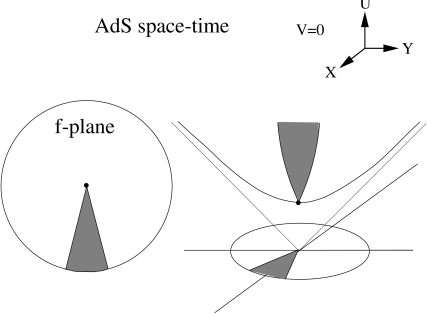
Figure 1: A particle located at the origin in AdS space-time.

If we have fixed the number of singularities there is still a residual symmetry left that can be used to move the singularity around on the Poincaré disk:

$$f\rightarrow g=\frac{\alpha f+\beta}{\bar{\beta}f+\bar{\alpha}}~{}~{}~{}~{}~{}\in SU(1,1)$$ (46)

SU(1,1) consists of three basic operations: one rotation and three boosts:

$$R(\vartheta) :\mbox{Rotation}:\alpha=e^{i\vartheta}~{}~{}~{}\beta=0$$ (47)

$$T_{x}(\xi) :\mbox{x-Boost}:\alpha=\cosh\frac{\xi}{2}~{}~{}~{}\beta=\sinh\frac{\xi}{2}$$ (48)

$$T_{y}(\xi) :\mbox{y-Boost}:\alpha=\cosh\frac{\xi}{2}~{}~{}~{}\beta=i\sinh\frac{\xi}{2}$$ (49)

On the Poincaré disc a boost is really a translation over a distance $d=\tanh\frac{\xi}{2}$. As we saw, for a particle in the origin the function $f(z)$ is multivalued (45). If we place a particle at the positive x-axis at a distance $\tanh\frac{\xi}{2}$ its monodromy is given by:

$$g\rightarrow T_{x}(\xi)R(\vartheta)T^{-1}_{x}(\xi)g~{}~{}~{}~{}\vartheta=2\pi(1-4Gm)$$ (50)

In terms of $\alpha$ and $\beta$:

$$T_{x}RT^{-1}_{x}:\alpha=\cos\vartheta+i\sin\vartheta\cosh\xi~{}~{}~{}\beta=-i\sin\vartheta\sinh\xi$$ (51)

The next simplest case we can try to solve is the two particle problem. We can use the SU(1,1) freedom to put one particle in the origin and the other at the positive x-axis at a distance $\tanh\frac{\xi}{2}$ from the origin. But we know the monodromy of the function $f(z)$:

$$f \rightarrow R(2\pi\mu_{1})f~{}~{}~{}~{}~{}~{}\mbox{at}~{}f=0$$ (52)

$$f \rightarrow T_{x}(\xi)R(2\pi\mu_{2})T^{-1}_{x}(\xi)f~{}~{}~{}~{}~{}~{}\mbox{at}~{}f=\tanh\frac{\xi}{2}$$ (53)

with $\mu_{n}=1-4Gm_{n}$. The fact that we try to solve the function $f(z)$ from the information contained in its monodromies is called the Riemann-Hilbert problem. It is deeply related to the theory of Fuchsian differential equations. One can show that $f(z)$ can be written as $\frac{y_{1}}{y_{2}}$ where $y_{i}(z)$ are the two independent solutions to the following differential equation ([22, 21, 8]):

$$y^{\prime\prime}+\frac{1}{4}(\frac{1-\mu_{1}^{2}}{z^{2}}+\frac{1-\mu_{2}^{2}}{(z-1)^{2}}+\frac{1-\mu_{1}^{2}-\mu_{2}^{2}+\mu_{\infty}^{2}}{z(z-1)})y=0$$ (54)

At the points $z=0,1,\infty$ this differential equation is singular, but the singularities are of a special type called Fuchsian singularities. In a local basis where the monodromy is diagonal at $z=z_{n}$ the singular behaviour of the two independent solutions is:

$$y_{1} \stackrel{{\scriptstyle z\rightarrow z_{1,2}}}{{\sim}} (z-z_{1,2})^{\frac{1}{2}(1+\mu_{1,2})}~{}~{}~{}~{}~{}y_{1}\stackrel{{\scriptstyle z\rightarrow\infty}}{{\sim}}(\frac{1}{z})^{-\frac{1}{2}(1+\mu_{\infty})}$$ (55)

$$y_{2} \stackrel{{\scriptstyle z\rightarrow z_{1,2}}}{{\sim}} (z-z_{1,2})^{\frac{1}{2}(1-\mu_{1,2})}~{}~{}~{}~{}~{}y_{2}\stackrel{{\scriptstyle z\rightarrow\infty}}{{\sim}}(\frac{1}{z})^{-\frac{1}{2}(1-\mu_{\infty})}$$ (56)

with $z_{1}=0$ and $z_{2}=1$ In order to produce the correct $\delta$-functions we want this singular behaviour locally to be the same as the behaviour we found in the case of one particle, so we may write:

$$\mu_{1,2}=1-4Gm_{1,2}~{}~{}~{}~{}~{}~{}\mu_{\infty}=1-4GH_{\bf tot}$$ (57)

where $H_{\bf tot}$ is the total energy of the system in the center of mass frame defined by:

$$\cos(4\pi GH_{\bf tot})=\cos(4\pi Gm_{1})\cos(4\pi Gm_{2})-\cosh{\xi}\sin(4\pi Gm_{1})\sin(4\pi Gm_{2})$$ (58)

If we use a coordinate system for which the monodromy for particle 1 is diagonal, the solution around particle 2 and around infinity is, by analytic continuation of the solution around particle 1, a linear combination of the $y_{i}$ defined in (55,56). As we saw, the solution to the Liouville equation is $f=\frac{y_{1}}{y_{2}}$. As the Liouville equation is nonlinear, the relative constant between $y_{1}$ and $y_{2}$ is important. This constant is determined by matching the monodromy (53) to the monodromy of $f=\frac{y_{1}}{y_{2}}$. Once this is done we find as a solution:

$$f(z)=z^{\mu_{1}}\coth\frac{\xi}{2}\frac{\tilde{F}[\frac{1}{2}(1+\mu_{\infty}+\mu_{1}-\mu_{2}),\frac{1}{2}(1-\mu_{\infty}+\mu_{1}-\mu_{2}),1+\mu_{1};z]}{\tilde{F}[\frac{1}{2}(1+\mu_{\infty}-\mu_{1}-\mu_{2}),\frac{1}{2}(1-\mu_{\infty}-\mu_{1}-\mu_{2}),1-\mu_{1};z]}$$ (59)

where:

$$\tilde{F}[a,b,c;z]=\frac{\Gamma(a)\Gamma(b)}{\Gamma(c)}F[a,b,c;z]$$ (60)

and $F$ denotes the hypergeometric function. Because the hypergeometric function has its singularities at $z=0,1,\infty$ the particles are located in these coordinates at $z=0,1$. They can however easily be moved to arbitrary locations by using the following transformation:

$$w=a_{1}+z(a_{2}-a_{1})$$ (61)

In the $f$-coordinate system the first particle is located at $|f|=0$. This fact can be checked by calculating $f(0)=0$ from (59) . We also deduced that the second particle was located at the fixed point of the SU(1,1) monodromy, i.e. at $x=\tanh\frac{\xi}{2},y=0$. If we use the analytic continuation of $F(a,b,c;z)$ in the neighbourhood of $z=1$ and evaluate $f(1)$ we indeed find:

$$f(1)=\tanh\frac{\xi}{2}$$ (62)

It is of course interesting to see where $f(\infty)$ is located in the $f$-plane. For this one uses the analytic continuation of $F(a,b,c;z)$ around infinity (or $w=\frac{1}{z}\rightarrow 0$) and one finds (see for instance [20], page 663):

$$f(\infty)=e^{4\pi iGm_{1}}\sqrt{\frac{\sin\{2\pi G(H+m_{1}+m_{2})\}\sin\{2\pi G(H+m_{1}-m_{2})\}}{\sin\{2\pi G(H-m_{1}-m_{2})\}\sin\{2\pi G(H-m_{1}+m_{2})\}}}$$ (63)

Notice that in the range $m_{1},m_{2},H\in[0,\frac{1}{4G}]$ we have $|f(\infty)|\geq 1$. But physical infinity is already at $|f|=1$, implying that our universe is open! If we take the limit $m_{1}\rightarrow H,~{}m_{2}\rightarrow 0,~{}\xi\rightarrow 0$ we find that $|f(\infty)|\rightarrow\infty$ which is the correct result for the one particle case.

Equation (58) is precisely equation (4.5) in [11] for the case of two particles in an open universe without a horizon. Steif finds that for different ranges of the masses $m_{i}$ and $\xi$ there are also solutions representing an open universe where the two particles are enclosed by a horizon and a closed universe with an additional image mass. It would be interesting to see whether our gauge supports these solutions too.

If we want to insert N particles on the Poincaré disc we need to solve the Riemann-Hilbert problem with N Fuchsian singularities. One line of attack is to write down a more general second order differential equation of the form: [8, 21, 22]:

$$y^{\prime\prime}+\frac{1}{4}\sum_{i}(\frac{1-\mu_{i}^{2}}{(z-z_{i})^{2}}+\frac{2\beta_{i}}{(z-z_{i})})y=0$$ (64)

The $\mu_{i}$ are again used to match the masses and the $\beta_{i}$, called accessory parameters, are to be determined by matching with the monodromy. The problem of finding the explicit solution is however frustrated by the appearance of apparent singularities. These are singularities of the differential equation but zero’s of the solution to that equation.

Another way to think about the general Riemann-Hilbert problem is to try to write down a first order matrix differential equation [18, 7]:

$$\partial Y=\sum_{i=1}^{N}\frac{A_{i}}{z-z_{i}}Y$$ (65)

where $A_{i}$ are constant matrices (possibly depending on the $a_{i}$) and $Y$ is a fundamental matrix of solutions. The Riemann-Hilbert problem is now equivalent to finding the matrices $A_{i}$, given the monodromy matrices and the local exponents at the particle singularities. Lappo-Danilevski was the first to solve this problem in terms of an infinite series of hyperlogarithms [19]. Although this proves that under certain reasonable assumptions there exist solutions, these solutions are of little practical value because of their enormous complexity.

4 Black Hole solution

Up till now we only considered point particles, but it is well known that in AdS space-time also black hole (BH) solutions exist [10, 11, 12]. In the case of particles we were concerned with a multivalued mapping function $f(z)$ having elliptic monodromy. But SU(1,1) also contains hyperbolic and parabolic transformations. It happens that the black hole of mass $M$ is characterized by the following hyperbolic monodromy:

$$f(z)\rightarrow\frac{\cosh\pi(\sqrt{8GM})~{}f(z)+\sinh\pi(\sqrt{8GM})}{\sinh\pi(\sqrt{8GM})~{}f(z)+\cosh\pi(\sqrt{8GM})}$$ (66)

We could of course also have chosen a rotated transformation to change the orientation of the BH. We could also easily move the BH to a different location by conjugating (66) by a boost. Our task is thus to find the multivalued function $f(z)$ with monodromy (66). For that we first diagonalize the SU(1,1) transformation.

$$f^{\prime}\rightarrow\frac{\cosh\pi(\sqrt{8GM})-\sinh\pi(\sqrt{8GM})}{\cosh\pi(\sqrt{8GM})+\sinh\pi(\sqrt{8GM})}f^{\prime}$$ (67)

where $f^{\prime}$ is $f$ in a diagonal basis. Next consider the function:

$$f^{\prime}=z^{i\alpha}~{}~{}~{}~{}~{}~{}~{}~{}\alpha\in R$$ (68)

After a full rotation we find:

$$f^{\prime}(e^{2\pi i})z=e^{-2\pi\alpha}f^{\prime}(z)$$ (69)

So if we take:

$$\alpha=\frac{-1}{2\pi}\ln(\frac{\cosh\pi(\sqrt{8GM})-\sinh\pi(\sqrt{8GM})}{\cosh\pi(\sqrt{8GM})+\sinh\pi(\sqrt{8GM})})=\sqrt{8MG}$$ (70)

then $f^{\prime}(z)$ has the correct monodromy. Transforming back to the old basis finally gives:

$$f(z)=\frac{1+z^{i\sqrt{8GM}}}{1-z^{i\sqrt{8GM}}}=i\cot(\sqrt{2GM}\ln z)$$ (71)

Next we shall study this function a bit more. First we invert relation (71) to:

$$z^{i\alpha}=\frac{f-1}{f+1}~{}~{}~{}~{}~{}~{}~{}\alpha=\sqrt{8GM}$$ (72)

Putting $z=re^{i\varphi}$ and $f=Re^{i\vartheta}$ we write:

$$e^{-\alpha\varphi}(\cos(\alpha\ln r)+i\sin(\alpha\ln r)=\frac{R^{2}-1}{R^{2}+1+2R\cos\vartheta}+i\frac{2R\sin\vartheta}{R^{2}+1+2R\cos\vartheta}$$ (73)

Taking $\vartheta=0,\pi$ (the real line on the f-disc) we get:

$$\vartheta=0,\pi:~{}~{}~{}r=e^{\frac{\pi}{\alpha}(2n+1)}~{}~{}~{}\varphi=\pm\frac{1}{\alpha}\ln(\frac{1+R}{1-R})$$ (74)

The conformal factor diverges at the edge of the disc: $R=1$. There we find:

$$R=1:~{}~{}~{}r=e^{\frac{\pi}{2\alpha}(2n+1)}~{}~{}~{}\varphi=\frac{-1}{\alpha}\ln(\tan\frac{|\vartheta|}{2})$$ (75)

where $\vartheta>0$ implies even values of $n$ and $\vartheta<0$ implies odd values of $n$. Putting this information together we find figure (2).

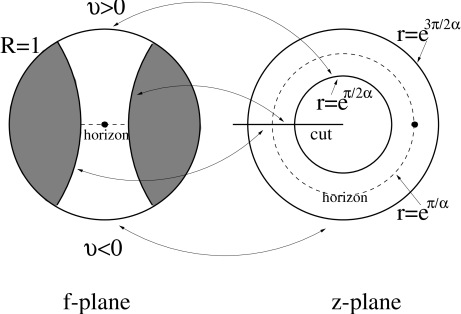
Figure 2: The mapping function $f(z)$ for a black hole.

On the $f$-plane one recognizes the BH geometry. The dotted line is the horizon (at $t=0$) Note that the location of infinity ($R=1$) in the interior region and exterior region of the BH are mapped to different circles on the z-plane. For a more detailed description of this BH solution represented on the Poincaré disc we refer to [12].

So we find that elliptic monodromy for the mapping function $f(z)$ gives a particle and hyperbolic monodromy a black hole. But what about the parabolic monodromy? In for instance [11] we find that this represents the black hole vacuum solution. One can either view this as the limit of a BH with zero mass or a particle with mass $1/4G$. It represents an infinitely long, and infinitely thin throat. The monodromy is given by:

$$f(z)\rightarrow\frac{(1+i\pi)f+\pi}{\pi f+(1-i\pi)}$$ (76)

The mapping function that exhibits this monodromy can be found by transforming this monodromy to Jordan form:

$$f^{\prime}(z)\rightarrow f^{\prime}(z)+2\pi i$$ (77)

and recognize the logarithm. Transforming back gives:

$$f(z)=i\frac{\ln z+1}{\ln z-1}$$ (78)

This mapping is depicted in figure (3).

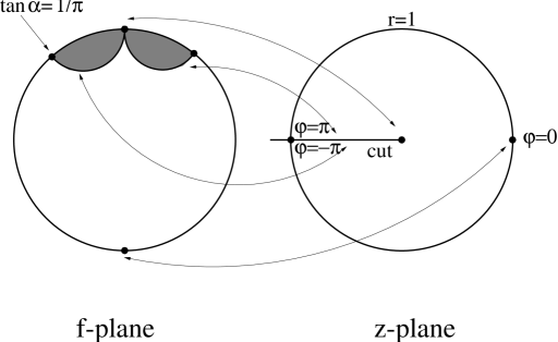
Figure 3: The mapping function $f(z)$ for a black hole vacuum solution.

The next step would be to search for mapping functions that describe multi BH states or combinations of BHs and particles. One should try to find mapping functions that exhibit prescribed monodromy properties. Only in this case we may have combinations of elliptic, hyperbolic and parabolic transformations! One could view this as a kind of generalized Riemann-Hilbert problem. Needless to say that the more BHs and particles one wants to describe the more complicated $f(z)$ gets. For the case of two ‘objects’ the equation that relates the masses is analogous to (58). For instance, in the case of two BHs we have [13]:

$$\cosh\pi(\sqrt{8GM_{\bf tot}})= -\cosh\pi(\sqrt{8GM_{1}})\cosh\pi(\sqrt{8GM_{2}})$$ (80)

$$+\cosh(\frac{d}{\ell})\sinh\pi(\sqrt{8GM_{1}})\sinh\pi(\sqrt{8GM_{2}})$$

where d is the distance between the horizons of the BHs. One recognizes that this is just an analytic continuation of (58) in the masses:

$$i\sqrt{8GM_{BH}}=1-4Gm_{P}$$ (81)

This suggests that the mapping function for two BHs will be some analytic continuation of (59) in the mass parameters $\mu_{i},\mu_{\infty}$. We did however not pursue this issue any further.

5 Closed surfaces and the Gauss-Bonnet theorem

In the previous sections we have seen how to accommodate particles and BHs in open spaces. But we could also decide to solve the Liouville equation on a closed surface $\Sigma$. Because in the general solution to the Liouville equation we still have an arbitrary analytic mapping function at our disposal, we expect that a large class of Riemann surfaces are solutions to the Liouville equation for $\Lambda<0$. There is however an important constraint on the possible configurations of particles and BHs living on a closed Riemann surface with constant negative curvature. Let’s call $g$ the number of BHs, N the number of BHVs and P the number of particles with mass $m_{P}$. The BH solutions have hyperbolic monodromy and are therefore represented as handles on the surface. The BHV solutions correspond to parabolic singularities (at infinity) and the particles correspond to elliptic (or conical or Fuchsian) singularities on $\Sigma$. The Gauss-Bonnet theorem tells us that the Euler characteristic can be related to the intrinsic curvature of the Riemann surface:

$$\chi(\Sigma)=\frac{1}{\pi}\int_{\Sigma}\sqrt{{}^{(2)}g}~{}^{(2)}R$$ (82)

Inserting the equation for the curvature (28) in the above equation and using the fact that $\chi(\Sigma)=2-2g$ gives:

$$2-2g = \frac{-1}{\pi}\int_{\Sigma}\nabla^{2}\phi$$ (83)

$$= \int_{\Sigma}(\frac{-1}{2\pi}e^{\phi}+\sum_{N}\delta^{2}(z-z_{N})+4G\sum_{P}m_{P}\delta^{2}(z-z_{P}))$$ (84)

Because $\int e^{\phi}=\int\sqrt{{}^{(2)}g}={\bf Area}(\Sigma)$ we find finally:

$${\bf Area}(\Sigma)=2\pi(2g-2+N+4G\sum_{P}m_{P})>0$$ (85)

So if there are no particles present, we would at least need 2 handles, or 1 handle and 1 parabolic singularity, or 3 parabolic singularities on a closed surface of constant negative curvature. This is precisely the content of the uniformization theorem on Riemann surfaces [16].

6 de Sitter Space-Time: $\Lambda>0$

In this section we want to consider briefly de Sitter space-time, i.e. $\Lambda=\frac{1}{\ell^{2}}>0$. We assume again that the metric is of the general form (23). The embedding in 3+1 dimensions is given by:

$$X = \ell\cosh\tau\sin\theta\cos\varphi$$ (86)

$$Y = \ell\cosh\tau\sin\theta\sin\varphi$$ (87)

$$Z = \ell\cosh\tau\cos\theta$$ (88)

$$T = \ell\sinh\tau$$ (89)

with:

$$X^{2}+Y^{2}+Z^{2}-T^{2}=\ell^{2}$$ (90)

So at negative time this represents a contracting sphere of radius $\ell\cosh\tau$, at $\tau=0$ the sphere has reached its minimal radius $\ell$ after which it will start to expand. The metric on de Sitter space is:

$$ds^{2} = -dT^{2}+dX^{2}+dY^{2}+dZ^{2}$$ (91)

$$= \ell^{2}(-d\tau^{2}+\cosh^{2}\tau(d\theta^{2}+\sin^{2}\theta d\varphi^{2}))$$ (92)

After defining again $t=\tau\ell$, $S(t)=\ell\cosh(\frac{t}{\ell})$ and $z=\tan\frac{\theta}{2}e^{i\varphi}$ this metric can be written as:

$$ds^{2}=-dt^{2}+\frac{4S^{2}(t)}{(1+z\bar{z})^{2}}dzd\bar{z}$$ (93)

The intrinsic and extrinsic curvature of the two surface is now given by:

$${}^{(2)}R = \frac{2}{S^{2}}=\frac{2}{\ell^{2}\cosh^{2}(\frac{t}{\ell})}$$ (94)

$$K = \frac{2}{\ell}\tanh(\frac{t}{\ell})$$ (95)

This solves the contracted Gauss-Codazzi equation (or equivalently the $00$-component of the Einstein equation):

$${}^{(2)}R+\frac{1}{2}K^{2}-\frac{2}{\ell^{2}}=0$$ (96)

If we allow for a more general conformal factor $e^{\phi(z,\bar{z})}$, then the Einstein equation for this factor is:

$$\partial\bar{\partial}\phi+\frac{1}{2}e^{\phi}=-4\pi G\sqrt{{}^{(2)}g}T^{00}$$ (97)

The Einstein equation for the scale factor $S(t)$ is precisely solved by $S=\ell\cosh(\frac{t}{\ell})$ if we assume time symmetry at $t=0$. The general solution for the slightly altered Liouville equation (97) is:

$$e^{\phi}=\frac{4\partial g~{}\bar{\partial}\bar{g}}{(1+g\bar{g})^{2}}$$ (98)

If we add one particle at $R^{2}\equiv g\bar{g}=0$ we can simply use the Ansatz $g(z)=(z)^{\mu}$ again and find: $\mu=1-4Gm$. After a coordinate transformation to static coordinates this turns out to be the solution found by Deser and Jackiw in [3]. In contrast with AdS space the metric does not blow up at $g\bar{g}=1$. If we calculate the distance from $R=0$ to $R=\infty$ at a constant time we find:

$$\Delta x=S(t)\int_{0}^{\infty}dR~{}\frac{2}{(1+R^{2})}=\pi S(t)$$ (99)

This implies that the singularity at $R=\infty$ is actually located at the opposite site of the sphere with radius $S(t)$, i.e. it is antipodal: see figure (4).

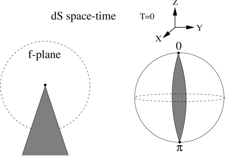
Figure 4: A particle located at the origin in dS space-time.

Adding more particles is only possible in even numbers therefore. In the case of $2N$ particles we are faced with a Riemann-Hilbert problem with $2N$ SU(2)-monodromies that cancel pairwise. It is obvious that the mapping function $g(z)$ will be very complicated in this case (although solvable in principle).

7 Discussion

In this paper we studied cosmologies of expanding or contracting matter in de Sitter, anti-de Sitter and Minkowski space-time. The AdS cosmologies correspond to the ones described by Steif and Brill [11, 12, 13], i.e. they are time symmetric at $t=0$. We found that the metric can be completely described in terms of a single factor composed of the product of a time-dependent scale $S(t)$ and space-dependent conformal factor $e^{\phi(x,y)}$. $S(t)$ describes the scale of the spatial surface at a time $t$. Amazing, and typical for gravity in 2+1 dimensions is that this scalefactor is not influenced by the matter content of the universe, i.e. it is the same for the vacuum solution and for a universe filled with mass. This is due to the topological nature of the interactions in 2+1 dimensions: there is no ‘real force’ acting on the masses. In other words, there are no gravitons to carry the interaction from one object to the other. The effect of the mass distribution is described the conformal factor $e^{\phi}$. The Einstein equations for this conformal factor translate into the Liouville equation for all three possibilities of the cosmological constant (dS space has however an extra minus sign in the equation). The solution of this Liouville equation is completely determined in terms of a single analytic function $f(z)$. So once we determine this mapping function for a matter distribution we know the complete metric and its time evolution. In 2+1 D AdS space-time there exist three kinds of massive object: point particles, black holes and black hole vacuum solutions. Note however that the black hole vacuum solution is not vacuum AdS space but an intermediate state between a particle and a black hole (a particle with mass $1/4G$ or a BH with zero mass). It happens that when we add these objects to AdS space the mapping function becomes multivalued. It has elliptic monodromy for particles, hyperbolic monodromy for BHs and parabolic monodromy for BHVs. So to find $f(z)$ for a combination of these three would result in Riemann-Hilbert problem with three types of monodromy [7, 8]. We found explicit solutions in the following cases:

$$\Lambda=0,\frac{-1}{\ell^{2}}$$ 1 particle, 2 particles, 1 BH, 1 BHV (100)

$$\Lambda=\frac{+1}{\ell^{2}}$$ 2 particles (101)

Notice that a 1 particle solution does not exist in dS space as a particle always has an antipode. The explicit solutions for AdS and Minkowski space-time represent open spatial surfaces (an open surface is defined as a surface with infinite area). In the case of dS space-time the spatial slice is always closed. In the last section we studied the possibility of closed surfaces in AdS and Minkowski space. Using the Gauss-Bonnet theorem we derive a simple inequality that determines which combinations of particles, BHs and BHVs can live in a closed space. This inequality is consistent with the uniformization theorem for Riemann surfaces. Finally we would like to comment on a possible application of the linearly expanding or contracting solution in the case of vanishing cosmological constant. It is well known that a serious complication in the calculation of a scattering amplitude using perturbation theory is that the particles are never free of ‘gravitational interaction’ in 2+1 D gravity. The interaction persists all the way to infinity because asymptotically the metric of a N particle solution is a cone and not Minkowski space. Actually the particles will be described for $t\rightarrow\infty$ by the metric (23) (with $S(t)\sim t$). The mapping function will be very complicated in the general case of N particles. Say however that we can define a wavefunction $\Psi_{\bf in}(z_{1},...z_{N})$ that describes this asymptotic state. On the Poicaré disc we have the angle at which the particle moves radially outward and the distance to the origin as a measure for its momentum. Then a possible definition for the scattering matrix is:

$$<\Psi_{\bf out}(z_{1},...,z_{N})|\Psi_{\bf in}(z_{1},...,z_{N})>$$ (102)

8 Acknowledgements

I would like to thank G. ’t Hooft and E. Verlinde for valuable suggestions and discussions.

References

- [1] Misner C W, Thorne K S and Wheeler J A 1973 Gravitation (San Francisco: W H Freeman and Company)
- [2] Deser S, Jackiw R and ’t Hooft G 1984 Ann Phys 152 220
- [3] Deser S and Jackiw R 1984 Ann Phys 153 405
- [4] ’t Hooft G 1992 Class Quant Grav 9 1335
- [5] Achucarro A and Townsend P 1986 Phys Lett B180 85
- [6] Witten E 1988 Nucl Phys B331 46
- [7] Welling M 1996 Class Quant Grav 13 653
- [8] Bellini A, Ciafaloni M and Valtancoli P 1995 Phys Lett B357 532, 1996 Nucl Phys B462 453
- [9] Ciafaloni M and Valtancoli P 1997 Class Quant Grav 14 955
- [10] Banãdos M, Teitelboim C and Zanelli J 1992 Phys Rev Lett 69 1849
- [11] Steif A R 1996 Phys Rev D53 5521
- [12] Brill D R 1996 Phys Rev D53 4133
- [13] Brill D R 1996 Geometry of Black Holes and Multi-Black-Holes in 2+1 dimensions gr-qc/9607026
- [14] Sachs R K 1964 Gravitational radiation in Relativity, Groups and Topology (Les Houches 1963) eds DeWitt C and DeWitt B (New York: Gordon and Breach)
- [15] Clément G 1994 Phys Rev D 50 7119
- [16] Matone M (1995) Int J Mod Phys A10 289
- [17] Plemelj J 1964 Problems in the sense of Riemann and Klein (London: John Wiley)
- [18] Sato M, Miwa T and Jimbo M 1979 in Complex Analysis, Microcalculus, and Relativistic Quantum Theory (Lecture Notes in Physics, vol 120) ed Lagolnitzer D (Berlin: Springer)
- [19] Chudnovsky D V 1979 Nonlinear Evolution Equations and Dynamical Systems (Lecture Notes in Physics, vol 120) ed Boiti M Pempinelli F and Soliani G (Berlin: Springer)
- [20] Sansone G and Gerretsen 1969 Lectures on the theory of functions of a complex variable II (Groningen: Wolters- Noordhoff)
- [21] Hille E 1976 Ordinary differential equations in the complex domain (New York: John Wiley & Sons)
- [22] Bieberbach L 1953 Theory der gewönlichen differentialgleichungen (Berlin: Springer)