NBI-HE-97-17

TIT/HEP-353

We construct a reparametrization invariant two-point function for $c=-2$ conformal matter coupled to two-dimensional quantum gravity. From the two-point function we extract the critical indices $\nu$ and $\eta$. The results support the quantum gravity version of Fisher’s scaling relation. Our approach is based on the transfer matrix formalism and exploits the formulation of the $c=-2$ string as an $O(n)$ model on a random lattice.

1 Introduction

Two-dimensional gravity has been a very useful laboratory for the study of interaction between matter and geometry. In particular, the so-called transfer matrix formalism [1, 2] has provided us with a new tool to analyse quantum geometry. It allows us to study the fractal structure of space time and using this formalism it has been possible to calculate a reparametrization invariant two-point function of pure gravity [3]. This two-point function has a number of nice properties [3]:

1. Both the short distance and the long distance behaviour of the two-point point function reflect directly the fractal structure of quantum space-time.

2. The two-point function makes possible a definition of a mass gap in two-dimensional quantum gravity.

3. In a regularised theory (e.g. two-dimensional quantum gravity defined by means of dynamical triangulations) this mass gap plays the same role as in the theory of critical phenomena: it monitors the approach to the critical point.

4. From the two-point function it is possible to define the same critical exponents as in the theory of critical phenomena, i.e.  the mass gap exponent $\nu$, the anomalous scaling exponent $\eta$ and the susceptibility exponent $\gamma_{\rm str}$.

5. Although the exponents take unusual values from the point of view of conventional field theory ($\eta=4$, $\gamma_{\rm str}=-1/2$), they nevertheless satisfy Fisher’s scaling relation $\gamma_{\rm str}=\nu(2-\eta)$.

More specifically, the renormalised two-point function of pure two-dimensional quantum gravity reads

$$G_{\Lambda}(D)=\Lambda^{3/4}\,\frac{\cosh(\sqrt[4]{\Lambda}\,D)}{\sinh^{3}(\sqrt[4]{\Lambda}\,D)},$$ (1.1)

where $D$ is the geodesic distance between two marked points. It is readily seen that the two-point function (1.1) (and its discretised version) satisfy the points 1.–5. [3]. We expect 1.–5. to be valid even if matter is coupled to quantum gravity, although with different critical exponents, and 1.–5. constitute the foundation of the successful application of finite size scaling in two-dimensional quantum gravity [4, 5, 6].

A major puzzle remains in two-dimensional quantum gravity. Formal constructions of a string field Hamiltonian for a $(m,m+1)$ conformal field theory coupled quantum gravity suggest that [7, 8]

$$d_{H}\equiv\frac{1}{\nu}=2m.$$ (1.2)

This relation can also be written as

$$d_{H}\equiv\frac{1}{\nu}=-\,\frac{2}{\gamma_{\rm str}}.$$ (1.3)

However, this relation has not been observed in the numerical simulations [4, 5]. A number of problems have so far blocked decisive comparison between the theoretical prediction (1.3) and the numerical simulations. The (internal) Hausdorff dimension (1.2) is so large that the systems used in the numerical simulations might not have detected it. Secondly, additional assumptions about the field content go into the formal derivation of (1.2) and in particular, the identification of the proper time $T$ of the string field Hamiltonian as the geodesic distance becomes questionable. We shall return to this point later, see also reference [9].

In this paper we determine the two-point function in the case where $c=-2$ matter is coupled to quantum gravity. As shown by David [10], the discrete version of the $c=-2$ string [11] can be mapped onto a zero-dimensional field theory via Parisi-Sourlas dimensional reduction [12]. This zero-dimensional field theory can be viewed as a special version of the $O(n)$ model on a random lattice [13]; namely one for which $n=-2$. Our construction of the two-point function for the system of $c=-2$ matter coupled to quantum gravity will be based on this equivalence with the $O(n)$ model. We start from the discretised version of the model and construct the transfer matrix in the spirit of [7, 8], but without any additional assumptions on the matter fields. The simplicity of the model allows us to determine the two-point function exactly. We extract the critical indices $\nu$ and $\eta$, verify that Fisher’s scaling relation is fulfilled and find that our results support the relation (1.3). At the same time the $c=-2$ string is a perfect model for numerical simulations and computer simulations allow a determination of $\nu$ with high precision.

The rest of this paper is organised as follows: in section 2 we construct a string field theory for a general loop gas model which contains the $O(n)$ model on a random lattice as a special case. Section 3 is devoted to the study of the $O(n)$ model itself and in section 4 we specialise to the case $n=-2$. Section 5 contains a detailed analysis of the $c=-2$ string and finally in section 6 we discuss the exact results obtained and compare with numerical results. We also comment on the implications of our results for the series of minimal unitary models coupled to quantum gravity.

2 Dynamical triangulations with coloured loops

The $O(n)$ model on a random lattice is an example of a so-called loop gas model. Loop gas models can be defined in very general settings (see for instance [14] and references therein) and play an important role in field theory as well as in statistical mechanics. Hence, although our final aim is to study the $O(n)$ model on a random lattice, we shall start out with a more general loop gas model.

2.1 The model

We consider the set of two-dimensional closed connected complexes obtained by gluing together $i$-gons ($i\geq 3$) along pairs of links. On these complexes we introduce coloured loops. The loops live on the dual complex and their links connect centres of neighbouring triangles belonging to the original complex. We restrict the loops to be closed, self-avoiding and non-intersecting and we assume that they come in $N_{c}$ different colours. We denote those triangles (links) in the complex which are traversed by loops as decorated triangles (links) and those not traversed by loops as non-decorated triangles (links). All $i$-gons with $i\geq 4$ are per definition non-decorated. We define the partition function of our model by

$$Z=\sum_{T\in{\cal T}}g_{s}^{h-1}\sum_{\{{\cal L}\}}\frac{1}{C_{T}(\{{\cal L}\})}\prod_{i\geq 3}g_{i}^{N_{i}}\prod_{a=1}^{N_{c}}\kappa_{a}^{l_{a}}\,\lambda_{a}^{n_{a}}$$ (2.1)

where ${\cal T}$ denotes the class of complexes described above, $T$ is a complex in ${\cal T}$ and $\{{\cal L}\}$ is a given loop configuration on $T$ obeying the above given rules. The quantity $C_{T}(\{{\cal L}\})$ is the order of the automorphism group of $T$ with the loop configuration $\{{\cal L}\}$. The quantity $h$ is the genus of the complex, $N_{i}$ the number of non-decorated $i$-gons and $n_{a}$ the number of loops of colour $a$. Finally $l_{a}$ is the total length of loops with colour $a$ which is equal to the number of decorated triangles carrying the colour $a$.

2.2 The string field theory

We shall now, corresponding to the model (2.1), write down a string field theory for strings consisting of only non-decorated links. To do so it is necessary to define a distance or a time variable on the complexes introduced above. There exist two different approaches to this problem, known as the slicing decomposition [1] and the peeling decomposition [2]. As it will become clear shortly the presence of the loops on the surfaces makes it an advantage to use the peeling decomposition. Let us consider a disk with a boundary consisting of $l$ non-decorated links, one of which is marked. Our minimal step decomposition will take place at the marked link. To describe the deformation we introduce string fields, $\psi^{\dagger}(l)$ and $\psi(l)$ which respectively creates and annihilates a closed string of non-decorated links having length $l$ and one marked link. The string fields obey the following commutation relations,

$$\left[\psi(l),\psi^{\dagger}(l^{\prime})\right] = \delta_{l,l^{\prime}}\,,$$ (2.2)

$$\left[\psi^{\dagger}(l),\psi^{\dagger}(l^{\prime})\right] = \left[\psi(l),\psi(l^{\prime})\right]=0\,.$$ (2.3)

Expressed in terms of the string fields we define our minimal step decomposition by 

$$\delta\psi^{\dagger}(l) = -\psi^{\dagger}(l)+\sum_{i=3}^{\infty}g_{i}\psi^{\dagger}(l+i-2)+\sum_{l^{\prime}=0}^{l-2}\psi^{\dagger}(l^{\prime})\psi^{\dagger}(l-l^{\prime}-2)$$ (2.7)

$$+\sum_{a=1}^{N_{c}}\lambda_{a}\sum_{m=0}^{\infty}\kappa_{a}^{m+1}\sum_{l^{\prime}=0}^{m}\left(\!\!\begin{array}[]{c}m\\ l^{\prime}\end{array}\!\!\right)\psi^{\dagger}(l^{\prime})\psi^{\dagger}(l+m-l^{\prime}-1)$$

$$+2g_{s}\sum_{l^{\prime}=1}^{\infty}\psi^{\dagger}(l+l^{\prime}-2)l^{\prime}\psi(l^{\prime}).$$

In case the marked link does not belong to a decorated triangle the minimal step decomposition of the surface is defined exactly as in the pure gravity case, i.e. the decomposition consists in removing either an $i$-gon or a double link [2]. The removal of an $i$-gon always increases the length of the string by $i-2$. (As explained in [2] double links are supplied when necessary.) The removal of a double link either results in the splitting of one string into two or the merging of two strings into one. In the latter case a handle is created. The creation of a handle is associated with a factor of $2g_{s}$. This accounts for the terms in the first and the third lines of (2.7). The term in the second line describes the minimal step decomposition in the case where the marked link belongs to a decorated triangle. This situation is illustrated in figure 1.

Figure 1: The minimal step decomposition in the case where the marked link belongs to a decorated triangle. The dotted line illustrates the loop.

Let us assume that the loop which passes through the triangle with the marked link has length $m+1$ ($m\geq 0$). It hence passes through $m+1$ triangles. Of these $m+1$ decorated triangles a certain number, say, $l^{\prime}$ will have their base on the inner side of the loop and the remaining $m+1-l^{\prime}$ triangles will have their base on the outer side of the loop. Our minimal step decomposition consists in removing all $m+1$ triangles along the loop so that the initial string of length $l$ is replaced by two new strings of length $l^{\prime}$ and $l+m-1-l^{\prime}$ respectively, see figure 1. A removed loop of colour $a$ is accompanied by a factor $\lambda_{a}$ and each removed triangle along the loop is accompanied by a factor $\kappa_{a}$. The factor $\left(\!\!\begin{array}[]{c}m\\ l^{\prime}\end{array}\!\!\right)$ counts the number of possible orientations of the triangles along the loop.

We now perform a discrete Laplace transformation of our creation and annihilation operators. The Laplace transformed versions of $\psi^{\dagger}(l)$ and $\psi(l)$ are defined by 

$$\psi^{\dagger}(p)=\sum_{l=0}^{\infty}\frac{1}{p^{l+1}}\,\psi^{\dagger}(l)\hskip 14.22636pt(|p|>p_{c}),\hskip 28.45274pt\psi(q)=\sum_{l=1}^{\infty}\frac{1}{q^{l+1}}\psi(l)\hskip 14.22636pt(|q|>q_{c}),$$ (2.8)

and we assume that these expressions make sense for $|p|$ and $|q|$ larger than some critical values $p_{c}$ and $q_{c}$ respectively. The inverse transformations to (2.8) can be written as

$$\psi^{\dagger}(l)=\oint_{|s|=p_{c}}\frac{ds}{2\pi i}s^{l}\,\psi^{\dagger}(s),\hskip 28.45274pt\psi(l)=\oint_{|s|=q_{c}}\frac{ds}{2\pi i}s^{l}\,\psi(s),$$ (2.9)

where the integrals can be evaluated by taking the residues at infinity. Here and in the following we use the convention that unless otherwise indicated contours are oriented counterclockwise. The Laplace transformed versions of the commutation relations (2.2) and (2.3) are

$$\left[\psi(q),\psi^{\dagger}(p)\right] = \frac{1}{pq(pq-1)},$$ (2.10)

$$\left[\psi^{\dagger}(p),\psi^{\dagger}(p^{\prime})\right] = \left[\psi(q),\psi(q^{\prime})\right]=0.$$ (2.11)

We here need to require $p_{c}q_{c}=1$. We next rewrite the string deformation equation (2.7) in the Laplace transformed language. This is most easily done by applying the operator $\sum_{l=1}^{\infty}\frac{1}{p^{l}}$ to both sides of (2.7). The treatment of the terms in the first and third lines is standard while the treatment of the term in the second line is less trivial. We have for $|p|>p_{c}$

$$I(p,\kappa) \equiv \sum_{l=1}^{\infty}\frac{1}{p^{l}}\sum_{m=0}^{\infty}\kappa^{m+1}\sum_{l^{\prime}=0}^{m}\left(\!\!\begin{array}[]{c}m\\ l^{\prime}\end{array}\!\!\right)\psi^{\dagger}(l^{\prime})\psi^{\dagger}(l+m-l^{\prime}-1)$$ (2.14)

$$= \oint_{|s|=p_{c}}\frac{ds}{2\pi i}\oint_{|s^{\prime}|=p_{c}}\frac{ds^{\prime}}{2\pi i}\,\frac{1}{p}\sum_{l=0}^{\infty}\left(\frac{s}{p}\right)^{l}\sum_{m=0}^{\infty}\kappa^{m+1}\sum_{l^{\prime}=0}^{m}\left(\!\!\begin{array}[]{c}m\\ l^{\prime}\end{array}\!\!\right)s^{\prime l^{\prime}}s^{m-l^{\prime}}\psi^{\dagger}(s)\psi^{\dagger}(s^{\prime})$$

$$= \oint_{|s|=p_{c}}\frac{ds}{2\pi i}\oint_{|s^{\prime}|=p_{c}}\frac{ds^{\prime}}{2\pi i}\frac{1}{p-s}\sum_{m=0}^{\infty}\kappa^{m+1}\left(s^{\prime}+s\right)^{m}\psi^{\dagger}(s)\psi^{\dagger}(s^{\prime})$$

$$= \oint_{|s|=p_{c}}\frac{ds}{2\pi i}\oint_{|s^{\prime}|=p_{c}}\frac{ds^{\prime}}{2\pi i}\frac{1}{p-s}\,\frac{1}{\frac{1}{\kappa}-\left(s^{\prime}+s\right)}\psi^{\dagger}(s)\psi^{\dagger}(s^{\prime}).$$ (2.18)

Here the last equality sign is only valid if $|\kappa(s+s^{\prime})|<1$. From this we learn that we must require

$$p_{c}<\min_{a}\left|\frac{1}{2\kappa_{a}}\right|$$ (2.19)

in order for the subsequent considerations to make sense. Stated otherwise the model becomes singular as $p_{c}\rightarrow\min_{a}\left|\frac{1}{2\kappa_{a}}\right|$. In equation (2.18) we can carry out the integration over $s^{\prime}$. This gives

$$I(p,\kappa)=\oint_{|s|=p_{c}}\frac{ds}{2\pi i}\frac{1}{p-s}\psi^{\dagger}(s)\psi^{\dagger}(\frac{1}{\kappa}-s).$$ (2.20)

We note that the product $\psi^{\dagger}(s)\psi^{\dagger}(\frac{1}{\kappa}-s)$ is ill defined in both of the regions $|s|<p_{c}$ and $|\frac{1}{\kappa}-s|<p_{c}$. Due to this fact we can not immediately perform the second integration. We shall show later how to deal with this problem. For the moment we note that we have

$$p\delta\psi^{\dagger}(p) = -\oint_{|s|=p_{c}}\frac{ds}{2\pi i}\frac{1}{p-s}V^{\prime}(s)\psi^{\dagger}(s)+\left(\psi^{\dagger}(p)\right)^{2}+\sum_{a=1}^{N_{c}}\lambda_{a}\,I(p,\kappa_{a})$$ (2.21)

$$+2g_{s}\!\!\oint\limits_{|s|=p_{c}}\!\!\!\frac{ds}{2\pi i}\frac{1}{p-s}\psi^{\dagger}(s)\frac{\partial}{\partial s}\left(\frac{1}{s}\psi(\frac{1}{s})\right)\,,$$

where we have made use of the following rewriting

$$-p\psi^{\dagger}(p)+1+\sum_{i=3}^{\infty}g_{i}p^{i-1}\left\{\psi^{\dagger}(p)-\sum_{l=0}^{i-2}\frac{1}{p^{l+1}}\psi^{\dagger}(l)\right\}=-\oint_{|s|=p_{c}}\frac{ds}{2\pi i}\frac{1}{p-s}V^{\prime}(s)\psi^{\dagger}(s)$$ (2.22)

with

$$V(s)=\frac{1}{2}s^{2}-\sum_{i=3}^{\infty}\frac{g_{i}}{i}s^{i}$$ (2.23)

and $V^{\prime}(s)=dV(s)/ds$. We now introduce an operator ${\cal H}$, a Hamiltonian, which describes the minimal step deformation of our surface or the time evolution of the wave function. More precisely we define ${\cal H}$ by

$$l\delta\psi^{\dagger}(l)=-\left[{\cal H},\psi^{\dagger}(l)\right],$$ (2.24)

with the vacuum condition

$${\cal H}|\mbox{vac}\rangle=0.$$ (2.25)

It is easy to see that ${\cal H}$ can be expressed in the following way

$${\cal H} = \sum_{l=1}^{\infty}l\delta\psi^{\dagger}(l)\psi(l)=\oint_{|s|=p_{c}}\frac{ds}{2\pi i}\delta\psi^{\dagger}(s)s\frac{\partial}{\partial s}\left(\frac{1}{s}\psi\left(\frac{1}{s}\right)\right)$$ (2.26)

$$= -\oint\limits_{|s|=p_{c}}\!\!\!\frac{ds}{2\pi i}\Biggl{[}\left\{-V^{\prime}(s)\psi^{\dagger}(s)+\left(\psi^{\dagger}(s)\right)^{2}+\sum_{a=1}^{N_{c}}\lambda_{a}\psi^{\dagger}(s)\psi^{\dagger}\left(\frac{1}{\kappa_{a}}-s\right)\right\}\frac{\partial}{\partial s}\left(\frac{1}{s}\psi\left(\frac{1}{s}\right)\right)$$

$$\hskip 71.13188pt+g_{s}\psi^{\dagger}(s)\left(\frac{\partial}{\partial s}\left(\frac{1}{s}\psi\left(\frac{1}{s}\right)\right)\right)^{2}\,\Biggr{]}\,.$$

Here we have arrived at a simple form of the contribution coming from the terms $I(p,\kappa_{a})$ in $p\delta\psi^{\dagger}(p)$ (cf. equation (2.21)) by changing the order of the two integrations. We note, however, that the simplification is only apparent. If we wanted to evaluate the contour integral in (2.26) explicitly we would again have to deal with the problem of the product $\psi^{\dagger}(s)\psi^{\dagger}\left(\frac{1}{\kappa}-s\right)$ being ill defined in both of the regions $|s|<p_{c}$ and $\left|\frac{1}{\kappa}-s\right|<p_{c}$.

2.3 The transfer matrix

We shall now introduce a transfer matrix which describes the propagation of a single string. For that purpose we need first to introduce the disk amplitude. The disk amplitude, $W(l)$, simply counts the number of possible triangulations of the disk, constructed in accordance with the rules of section 2.1, with one boundary component consisting of $l$ non-decorated links one of which is marked. In the string field theory language it is given by

$$W(l)=\lim_{t\rightarrow\infty}\langle\mbox{vac}|e^{-t{\cal H}_{\rm disk}}\psi^{\dagger}(l)|\mbox{vac}\rangle,$$ (2.27)

where ${\cal H}_{\rm disk}\equiv\left.{\cal H}\right|_{g_{s}=0}$ and $t$ can be thought of as measuring the time evolving as the string field propagates or the distance being covered as the surface is decomposed (peeled). Its Laplace transform,

$$W(p)=\sum_{l=0}^{\infty}\frac{1}{p^{l+1}}\,W(l)=\lim_{t\rightarrow\infty}\langle\mbox{vac}|e^{-t{\cal H}_{\rm disk}}\psi^{\dagger}(p)|\mbox{vac}\rangle,$$ (2.28)

is the so-called one-loop correlator. Next, we define a modified Hamiltonian, $\overline{{\cal H}}$, which generates the time evolution of a single string

$$\overline{{\cal H}}=\sum_{l=1}^{\infty}\psi^{\dagger}(l)\left\{\left.\frac{\delta{\cal H}_{\rm disk}}{\delta\psi^{\dagger}(l)}\right|_{\psi^{\dagger}(l)\rightarrow W(l)}\right\}.$$ (2.29)

In the Laplace transformed picture we have

$$\overline{{\cal H}}=\left.-\oint_{|s|=p_{c}}\frac{ds}{2\pi i}\right\{-V^{\prime}(s)\phi^{\dagger}(s)+2W(s)\phi^{\dagger}(s)$$ (2.30)

$$\hskip 17.07182pt\left.+\sum_{a=1}^{N_{c}}\lambda_{a}\left[W\left(\frac{1}{\kappa_{a}}-s\right)\phi^{\dagger}(s)+W(s)\phi^{\dagger}\left(\frac{1}{\kappa_{a}}-s\right)\right]\right\}\frac{\partial}{\partial s}\left(\frac{1}{s}\psi\left(\frac{1}{s}\right)\right)$$

where

$$\phi^{\dagger}(p)=\psi^{\dagger}(p)-\frac{1}{p}$$ (2.31)

i.e. we have excluded the trivial mode corresponding to a string of zero length. We now define the transfer matrix for one-string propagation by

$$G(p,q,t)=\langle\mbox{vac}\left|\psi(q)e^{-t\overline{{\cal H}}}\phi^{\dagger}(p)\right|\mbox{vac}\rangle.$$ (2.32)

Differentiation with respect to $t$ gives

$$\frac{\partial}{\partial t}G(p,q,t)=-\langle\mbox{vac}\left|\psi(q)e^{-t\overline{{\cal H}}}\left[\overline{{\cal H}},\phi^{\dagger}(p)\right]\right|\mbox{vac}\rangle.$$ (2.33)

Using the commutation relations (2.10) and (2.11) we find

$$\left[\overline{{\cal H}},\phi^{\dagger}(p)\right]=\left[\overline{{\cal H}},\psi^{\dagger}(p)\right]$$ (2.34)

$$= \frac{\partial}{\partial p}\left(-\oint_{|s|=p_{c}}\frac{ds}{2\pi i}\frac{1}{p-s}V^{\prime}(s)\phi^{\dagger}(s)+2W(p)\phi^{\dagger}(p)+\sum_{a=1}^{N_{c}}\lambda_{a}J(p,\kappa_{a})\right)$$

where

$$J(p,\kappa)=\oint_{|s|=p_{c}}\frac{ds}{2\pi i}\,\frac{1}{p-s}\left\{W\left(\frac{1}{\kappa}-s\right)\phi^{\dagger}(s)+W(s)\phi^{\dagger}\left(\frac{1}{\kappa}-s\right)\right\}\,.$$ (2.35)

Inserting (2.34) into (2.33) we get

$$\frac{\partial}{\partial t}G(p,q,t) = -\frac{\partial}{\partial p}\left(-\oint_{|s|=p_{c}}\frac{ds}{2\pi i}\frac{1}{p-s}V^{\prime}(s)G(s,q,t)+2W(p)G(p,q,t)\right.$$ (2.36)

$$+\left.\sum_{a=1}^{N_{c}}\lambda_{a}\langle\mbox{vac}\left|\psi(q)e^{-t\overline{{\cal H}}}J(p,\kappa_{a})\right|\mbox{vac}\rangle\right).$$

We see that the problem encountered in equation (2.20) and (2.26) still persists. The integrand in (2.35) is ill defined in the region $\left|\frac{1}{\kappa}-s\right|<p_{c}$ as well as in the region $|s|<p_{c}$. Let us now finally discuss how to deal with this problem. First we note that the structure of the integrand in (2.20) and (2.35) is similar. The integrand consists of a pole term and a factor which is invariant under the change $s\rightarrow\frac{1}{\kappa}-s$. Such integrals have an important symmetry. To expose this symmetry, let us deform the contour of integration into two new ones; one which encircles the point $s=\frac{1}{\kappa}$ at the appropriate distance, given by $|s-1/\kappa|=p_{c}$ and one which encircles the pole $s=p$, see figure 2.

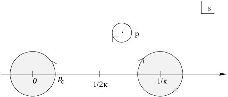
Figure 2: Deformation of the contour of integration in integrals of the type (2.18) and (2.35). The shaded regions are forbidden regions for $p$.

Then we get for, say $J(p,\kappa)$

$$J(p,\kappa)=\phi^{\dagger}(p)W\left(\frac{1}{\kappa}-p\right)+\phi^{\dagger}\left(\frac{1}{\kappa}-p\right)W(p)+\hat{J}(p,\kappa)$$ (2.37)

where we have simply picked up the residue at the pole $s=p$ and where $\hat{J}(p,\kappa)$ is given by

$$\hat{J}(p,\kappa)=-\oint_{|\frac{1}{\kappa}-s|=p_{c}}\frac{ds}{2\pi i}\,\frac{1}{p-s}\left\{W\left(\frac{1}{\kappa}-s\right)\phi^{\dagger}(s)+W(s)\phi^{\dagger}\left(\frac{1}{\kappa}-s\right)\right\}.$$ (2.38)

Now performing the change of variable $s\rightarrow\frac{1}{\kappa}-s$ in (2.38) one finds

$$\hat{J}(p,\kappa)=-J\left(\frac{1}{\kappa}-p,\kappa\right).$$ (2.39)

It is easy to see that a similar symmetry is encoded in any integral with the structure characterised above. In this connection, let us add a comment on the analyticity structure of equation (2.37). The first two terms on the right hand side are well defined only if both the conditions $|p|>p_{c}$ and $\left|\frac{1}{\kappa}-p\right|>p_{c}$ are fulfilled while the third term is well defined if $\left|\frac{1}{\kappa}-p\right|>p_{c}$. The sum of the three terms, however, is well defined if $|p|>p_{c}$. Exploiting the symmetry (2.39) one can, in certain special cases, by taking a linear combination of different versions of equation (2.36), with suitably chosen values for the parameter $p$, eliminate the terms depending on $J(p,\kappa)$. In the following section we shall see how this works for the $O(n)$ model on a random lattice and leads to an exactly solvable differential equation for the transfer matrix in the case $n=-2$.

3 The $O(n)$ model on a random lattice

The $O(n)$ model on a random lattice corresponds to the following special case of the general loop gas model (2.1)

$$N_{c}=n,\hskip 19.91684pt\kappa_{1}=\ldots=\kappa_{n}=\kappa,\hskip 19.91684pt\lambda_{1}=\ldots=\lambda_{n}=1$$ (3.1)

or equivalently

$$N_{c}=1,\hskip 19.91684pt\kappa_{1}=\kappa,\hskip 19.91684pt\lambda_{1}=n.$$ (3.2)

In this case the surface decomposition that we have presented in section 2.2 is equivalent to the one used in [15] to give a combinatorial derivation of the Dyson-Schwinger equations for the $O(n)$ model on a random lattice. Obviously these Dyson-Schwinger equations are contained in the string field theory formulation. They can be extracted as explained in [2]. Furthermore, our string field deformation is similar in nature to the one presented in [7] although in this reference several string fields are introduced. For the $O(n)$ model on a random lattice the existence of a singularity as $p_{c}\rightarrow\frac{1}{2\kappa}$ (cf. page 2.19) is well-known and the analyticity structure depicted in figure 2 is completely equivalent to the double cut nature of the saddle point equation encountered in the matrix model formulation of the model [13, 16, 17, 18, 19].

In the following we shall make the restriction

$$g_{4}=g_{5}=\ldots=0.$$ (3.3)

It is well known that when $n\in[-2,2]$ the $O(n)$ model on a random lattice has a plethora of critical points at which the scaling behaviour can be identified as that characteristic of conformal matter fields coupled to two-dimensional quantum gravity [13, 15, 16, 17, 18]. With a general potential any minimal conformal model can be reached. With the restriction (3.3) still all minimal unitary models are within reach. We make this restriction in order to obtain a simple contribution from the contour integral term in the differential equation (2.36). For the $O(n)$ model on a random lattice given by the above choice of parameters, (2.36) reduces to

$$\frac{\partial}{\partial t}G(p,q,t)=-\frac{\partial}{\partial p}\left(\left[-V^{\prime}(p)+2W(p)\right]G(p,q,t)+n\langle\mbox{vac}|\psi(q)e^{-t\overline{\cal H}}J(p,\kappa)|\mbox{vac}\rangle\right).$$ (3.4)

Now, inserting (2.37) and (2.39) into (2.36) we arrive at

$$\frac{\partial}{\partial t}G(p,q,t)=-\frac{\partial}{\partial p}\left(\left[-V^{\prime}(p)+2W(p)+nW\left(\frac{1}{\kappa}-p\right)\right]G(p,q,t)\right.$$ (3.5)

$$\left.+nW(p)G\left(\frac{1}{\kappa}-p,q,t\right)-n\langle\mbox{vac}\Big{|}\psi(q)e^{-t\overline{{\cal H}}}J\left(\frac{1}{\kappa}-p,\kappa\right)\Big{|}\mbox{vac}\rangle\right).$$

Hence we see that by subtracting from equation (3.5) the equation (2.36) with $p$ replaced by $\frac{1}{\kappa}-p$ we can eliminate the term involving $J\left(\frac{1}{\kappa}-p,\kappa\right)$. The resulting equation reads

$$\frac{\partial}{\partial t}\left\{G(p,q,t)-G\left(\frac{1}{\kappa}-p,q,t\right)\right\}=$$ (3.6)

$$-\frac{\partial}{\partial p}\left\{\left[-V^{\prime}(p)+2W(p)+nW\left(\frac{1}{\kappa}-p\right)\right]G(p,q,t)\right.$$

$$+\left.\left[-V^{\prime}(\frac{1}{\kappa}-p)+2W\left(\frac{1}{\kappa}-p\right)+nW(p)\right]G\left(\frac{1}{\kappa}-p,q,t\right)\right\}.$$

As we shall see in the following section for $n=-2$ and for a certain class of potentials this equation contains enough information that the complete transfer matrix can be extracted. We note that for $n\neq\pm 2$ we can write

$$\frac{\partial}{\partial t}\left\{G(p,q,t)-G\left(\frac{1}{\kappa}-p,q,t\right)\right\}=$$ (3.7)

$$-\frac{\partial}{\partial p}\left\{\left[2W_{s}(p)+nW_{s}\left(\frac{1}{\kappa}-p\right)\right]G(p,q,t)\right.$$

$$+\left.\left[2W_{s}\left(\frac{1}{\kappa}-p\right)+nW_{s}(p)\right]G\left(\frac{1}{\kappa}-p,q,t\right)\right\}$$

where $W_{s}(p)$ is the singular part of the disk amplitude, defined by

$$W(p)=W_{r}(p)+W_{s}(p)$$ (3.8)

with

$$W_{r}(p)=\frac{2V^{\prime}(p)-nV^{\prime}(\frac{1}{\kappa}-p)}{4-n^{2}}.$$ (3.9)

4 The $O(-2)$ model

Let us split the transfer matrix into two components in the following way

$$G(p,q,t)=\frac{1}{2}\left\{G_{+}(p,q,t)+G_{-}(p,q,t)\right\}$$ (4.10)

where

$$G_{\pm}(p,q,t)=G(p,q,t)\pm G\left(\frac{1}{\kappa}-p,q,t\right).$$ (4.11)

The functions $G_{+}(p,q,t)$ and $G_{-}(p,q,t)$ are respectively symmetric and antisymmetric under the transformation $p\rightarrow\frac{1}{\kappa}-p$, i.e.

$$G_{\pm}(p,q,t)=\pm G_{\pm}(\frac{1}{\kappa}-p,q,t).$$ (4.12)

Now, let us restrict ourselves to considering an antisymmetric potential, i.e. let us assume that

$$V^{\prime}(p)=-V^{\prime}\left(\frac{1}{\kappa}-p\right).$$ (4.13)

As for generic $n$, in order to obtain a simple contribution from the the contour integration term in the differential equation (2.36) we furthermore restrict the degree of the potential. In this case it is sufficient to require

$$g_{5}=g_{6}=\ldots=0.$$ (4.14)

(We note that the relations (4.13) and (4.14) leave only one free parameter for the potential.) Then it appears that for $n=-2$ the differential equation (2.36) turns into a closed equation for $G_{-}(p,q,t)$, namely

$$\frac{\partial}{\partial t}G_{-}(p,q,t)=-\frac{\partial}{\partial p}\left\{\left(-V^{\prime}(p)+2W_{-}(p)\right)G_{-}(p,q,t)\right\}$$ (4.15)

where in analogy with (4.11) we have introduced

$$W_{\pm}(p)=W(p)\pm W\left(\frac{1}{\kappa}-p\right).$$ (4.16)

As initial condition we have

$$G_{-}(p,q,t=0)=\frac{1}{pq(pq-1)}-\frac{1}{\left(\frac{1}{k}-p\right)q\left(\left(\frac{1}{\kappa}-p\right)q-1\right)}.$$ (4.17)

The differential equation (4.15) allows us to determine the odd part of the transfer matrix and as we shall show shortly the analyticity structure of the problem allows us to extract from $G_{-}(p,q,t)$ the function $G_{+}(p,q,t)$ and therefore the full transfer matrix. (We note that the argument is not specific to the case $n=-2$ but $n=-2$ is the only case where we have a closed equation for $G_{-}(p,q,t)$.) The full transfer matrix $G(p,q,t)$ is well defined for any $|p|>p_{c}$ while its two components $G_{+}(p,q,t)$ and $G_{-}(p,q,t)$ are well defined only if we have both $|p|>p_{c}$ and $|1/{\kappa}-p|>p_{c}$. It follows from the matrix model calculations and equation (4.15) that the singularities of $G(p)$ (where for simplicity we have suppressed the dependence on $q$ and $t$) manifest themselves in the form of cuts. Let us assume that $G(p)$ has only one cut $[x,y]$. Then the functions $G_{+}(p)$ and $G_{-}(p)$ both have two cuts, namely $[x,y]$ and $[\frac{1}{\kappa}-y,\frac{1}{\kappa}-x]$. To express $G_{+}(p,q,t)$ in terms of $G_{-}(p,q,t)$ we follow the line of reasoning of reference [19]. First, we express the fact that $G(p)$ is analytic along the interval $[1/\kappa-y,1/\kappa-x]$

$$G_{+}(p+i0)+G_{-}(p+i0)=G_{+}(p-i0)+G_{-}(p-i0)\,,\hskip 14.22636ptp\in[1/\kappa-y,1/\kappa-x].$$ (4.18)

Using the parity condition (4.12) this can also be written as

$$G_{+}(p-i0)-G_{+}(p+i0)=G_{-}(p-i0)-G_{-}(p+i0)\,,\hskip 19.91684ptp\in[x,y].$$ (4.19)

Now, for any complex $p$ not belonging to the intervals $[x,y]$ and $[\frac{1}{\kappa}-y,\frac{1}{\kappa}-x]$ we can write $G_{+}(p)$ as (cf. figure 3)

Figure 3: Analyticity structure of $G_{+}(p)$ and $G_{-}(p)$ and the recipe for going from one to the other (cf. eqn. (4.20)).

$$G_{+}(p) = \oint_{C_{0}}\frac{d\omega}{2\pi i}\frac{1}{p-\omega}G_{+}(\omega)=\frac{1}{2}\oint_{C_{0}\cup C_{1}}\frac{d\omega}{2\pi i}\,\frac{1/\kappa-2\omega}{\left(1/\kappa-p-\omega\right)(p-\omega)}G_{+}(\omega)$$ (4.20)

$$= \frac{1}{2}\int_{C_{+}\cup C_{-}}\frac{d\omega}{2\pi i}\,\frac{1/\kappa-2\omega}{\left(1/\kappa-p-\omega\right)(p-\omega)}G_{+}(\omega)$$

$$= \oint_{C_{-}}\frac{d\omega}{2\pi i}\,\frac{1/\kappa-2\omega}{\left(1/\kappa-p-\omega\right)(p-\omega)}G_{+}(\omega)$$

$$= \oint_{C_{-}}\frac{d\omega}{2\pi i}\,\frac{1/\kappa-2\omega}{\left(1/\kappa-p-\omega\right)(p-\omega)}G_{-}(\omega)$$

where the last equality sign follows from (4.19) and the one before that from the parity condition (4.12). Hence, once we know $G_{-}(p)$ we can determine $G_{+}(p)$. Adding the two eliminates the cut $[\frac{1}{\kappa}-y,\frac{1}{\kappa}-x]$ and produces the full transfer matrix $G(p)$. Let us mention that by arguments analogous to those above one can also express $G_{-}(p)$ via a contour integral involving $G_{+}(p)$, namely

$$G_{-}(p)=\oint_{C_{-}}\frac{d\omega}{2\pi i}\,\frac{1/\kappa-2p}{\left(1/\kappa-p-\omega\right)(p-\omega)}G_{+}(\omega).$$ (4.21)

In order to determine the inverse Laplace transform of $G(p)$ i.e. in order to determine the generating function for the loop-loop amplitudes it is sufficient to know $G_{-}(p)$; namely

$$G(l)=\oint_{C_{-}}\frac{dp}{2\pi i}\,p^{l}G_{-}(p)$$ (4.22)

which follows immediately from the definition (4.10). We note that the relations (4.20), (4.21) and (4.22) are true for any function with an analyticity structure similar to that of $G(p)$.

5 The $c=-2$ string

As already mentioned the discrete version of the $c=-2$ string can by means of Parisi-Sourlas dimensional reduction be mapped onto a zero-dimensional field theory which can be viewed as a special version of the $O(n)$ model on a random lattice [10]. More precisely one has to take $n=-2$ and the potential to be of the form

$$V(p)=\frac{1}{2}(p-\kappa p^{2})^{2}\,,$$ (5.1)

which means that $g_{3}=3\kappa$, $g_{4}=-2\kappa^{2}$, and otherwise $g_{i}=0$. A continuum limit can be defined when $\kappa$ approaches one of its critical values $\kappa_{c}=\pm\frac{1}{8}$. We note that the potential has exactly the properties assumed in equation (4.13) and (4.14).

5.1 The disk amplitude

The disk amplitude $W_{-}(p)$ which enters the differential equation (4.15) can be found in several references, see for instance [10, 17, 19]. It can also be derived entirely within the string field theory framework generalising the ideas of reference [2]. One has

$$W_{-}(p)-\frac{1}{2}V^{\prime}(p)=-\kappa^{2}(p-\frac{1}{2\kappa})\sqrt{(p-x)(p-y)(p-1/\kappa+x)(p-1/\kappa+y)}$$ (5.2)

where

$$x=\frac{1}{2\kappa}-\left(\frac{1}{4\kappa^{2}}+\frac{2}{\kappa}\right)^{1/2},\hskip 28.45274pty=\frac{1}{2\kappa}-\left(\frac{1}{4\kappa^{2}}-\frac{2}{\kappa}\right)^{1/2}.$$ (5.3)

We shall be interested in studying the model in the vicinity of the critical point $\kappa_{c}=\frac{1}{8}$. (We choose to consider $\kappa_{c}>0$ since this gives us positive values for the amplitudes.) In this region of the parameter space we have $x<y\leq\frac{1}{2\kappa}\leq\frac{1}{\kappa}-y<\frac{1}{\kappa}-x$. The square root in (5.2) is defined so that its cuts are $[x,y]$ and $[1/\kappa-y,1/\kappa-x]$ and so that it is positive as $p\rightarrow\infty$. In particular this implies that the square root is negative for $p\in\,]y,1/{\kappa}-y[$. We note that the cut structure of (5.2) is exactly as depicted in figure 3 and that the critical point corresponds to the situation where the two cuts merge.

Let us now proceed to taking the continuum limit. To do so we must scale the coupling constant, $\kappa$, which is the discrete analogue of the cosmological constant, towards its critical value. We choose the following prescription

$$\kappa=\kappa_{c}e^{-\epsilon^{2}\Lambda}$$ (5.4)

where $\Lambda$ is the continuum cosmological constant and $\epsilon^{2}$ is a scaling parameter with the dimension of volume. Given the scaling of $\kappa$ the boundary equations (5.3) tell us how $x$ and $y$ will behave in the scaling limit. We have

$$y=\frac{1}{2\kappa_{c}}(1-\epsilon\,\sqrt{\Lambda}+{\cal O}(\epsilon^{3})),\hskip 28.45274ptx=\frac{1}{2\kappa_{c}}(1-\sqrt{2}+{\cal O}(\epsilon^{2})).$$ (5.5)

In order to get a non-trivial scaling of the one-loop correlator we must likewise scale $p$ to $\frac{1}{2\kappa_{c}}$ and this must be done in such a way that $p$ always remains inside the region of convergence of $W_{-}(p)$. We set

$$p=p_{c}e^{\epsilon\,\sigma},~{}~{}~{}~{}p_{c}=\frac{1}{2\kappa_{c}},$$ (5.6)

where we note that in case $\sigma$ is real it must belong to the interval $[-\sqrt{\Lambda},\sqrt{\Lambda}]$. Then we find for the one-loop correlator,

$$W_{-}(p)-\frac{1}{2}V^{\prime}(p)=\epsilon^{2}\sqrt{2}\,\sigma\sqrt{\Lambda-\sigma^{2}}+{\cal O}(\epsilon^{3})$$ (5.7)

and we define its continuum version, $W_{-}(\sigma)$, by

$$W_{-}(\sigma)=\lim_{\epsilon\rightarrow 0}\frac{1}{\sqrt{2}\epsilon^{2}}\left(W_{-}(p)-\frac{1}{2}V^{\prime}(p)\right)=\sigma\sqrt{\Lambda-\sigma^{2}}.$$ (5.8)

Here the square root is defined so that it has two cuts, $[-\infty,-\sqrt{\Lambda}]$ and $[\sqrt{\Lambda},\infty]$ and so that it is positive for $\sigma\in\,]\!-\sqrt{\Lambda},\sqrt{\Lambda}[$. This structure is dictated by the original definition of the square root in (5.2). Let us note that while $W_{-}(p)$ and $W_{+}(p)$, whether in their discrete or continuum version, both have two cuts, the full one-loop correlator of course has only one cut. Exactly as for the transfer matrix there exist contour integral formulas which connect $W_{+}(p)$ and $W_{-}(p)$ (cf. equation (4.20) and (4.21)). i.e. $\gamma_{\rm str}=-1$.

5.2 The transfer matrix

We shall now explicitly determine the transfer matrix for the $c=-2$ string by solving the differential equation (4.15). For simplicity we will work in the continuum language. In the previous section we have shown how to take the continuum limit of the one-loop correlator. Let us now discuss how to take the continuum limit of the remaining terms in equation (4.15). As regards the arguments of $G_{-}(p,q,t)$, obviously the scaling of $p$ is dictated by the relation (5.6). The scaling of $q$, on the other hand, is determined by the fact that the transfer matrix must obey a simple composition law [1] and reads

$$q=q_{c}e^{\epsilon\,\tau}\,,~{}~{}~{}~{}q_{c}=\frac{1}{p_{c}}=2\kappa_{c}\,.$$ (5.9)

The necessary scaling of $t$, the distance or time evolution parameter, then follows from the structure of the differential equation. We see that $t$ must behave as $t\sim\epsilon^{-1}\,T$ in order for equation (4.15) to be consistent and we set

$$t=\frac{p_{c}}{2\sqrt{2}\epsilon}\,T.$$ (5.10)

In particular we see that $T$ has the dimension of (volume)^1/2. Inserting the scaling relations (5.6) and (5.9) into the initial condition (4.17) we see that it is natural to introduce a continuum version of the transfer matrix by

$$G(p,q,t)\rightarrow\frac{1}{\epsilon}G(\sigma,\tau,T)$$ (5.11)

and from (5.6) it follows that the parity condition (4.12) turns into

$$G_{\pm}(\sigma,\tau,T)=\pm G_{\pm}(-\sigma,\tau,T).$$ (5.12)

Collecting everything we can write our differential equation as

$$\frac{\partial}{\partial T}G_{-}(\sigma,\tau,T) = -\frac{\partial}{\partial\sigma}\left(W_{-}(\sigma)\,G_{-}(\sigma,\tau,T)\right),$$ (5.13)

$$G_{-}(\sigma,\tau,T=0) = \frac{2\sigma}{\sigma^{2}-\tau^{2}}$$ (5.14)

where $\sigma$ has to belong to the region of analyticity of the square root, i.e. $\sigma$ must lie outside the intervals $[-\infty,-\sqrt{\Lambda}]$ and $[\sqrt{\Lambda},\infty]$. The procedure for solving an equation like (5.13) is standard. The solution is given by

$$G_{-}(\sigma,\tau,T)=\frac{W_{-}(\hat{\sigma})}{W_{-}(\sigma)}\,G_{-}(\hat{\sigma},\tau,T=0)=\frac{\hat{\sigma}\,\sqrt{\Lambda-\hat{\sigma}^{2}}}{\sigma\,\sqrt{\Lambda-\sigma^{2}}}\,\frac{2\hat{\sigma}}{\hat{\sigma}^{2}-\tau^{2}}$$ (5.15)

where $\hat{\sigma}=\hat{\sigma}(\sigma,T)$ is a solution of the characteristic equation

$$\frac{\partial}{\partial T}\,\hat{\sigma}(\sigma,T)=-\hat{\sigma}\sqrt{\Lambda-\hat{\sigma}^{2}}$$ (5.16)

with boundary condition

$$\hat{\sigma}(\sigma,T=0)=\sigma.$$ (5.17)

The equations (5.16) and (5.17) imply

$$T=-\int_{\sigma}^{\hat{\sigma}(\sigma,T)}\frac{d\sigma^{\prime}}{\sigma^{\prime}\sqrt{\Lambda-\sigma^{\prime 2}}}=\left[\frac{1}{\sqrt{\Lambda}}\log\left(\frac{\sqrt{\Lambda}+\sqrt{\Lambda-\sigma^{\prime 2}}}{\sigma^{\prime}}\right)\right]^{\hat{\sigma}(\sigma,T)}_{\sigma}\,.$$ (5.18)

From the integral in (5.18) we conclude that in case $\sigma$ is real (and hence belongs to the interval $[-\sqrt{\Lambda},\sqrt{\Lambda}]$) we have $\hat{\sigma}(T)<\hat{\sigma}(0)=\sigma$. From (5.18) we get

$$\hat{\sigma}(\sigma,T)=\frac{\sigma}{\cosh(\sqrt{\Lambda}T)+\sqrt{1-\frac{\sigma^{2}}{\Lambda}}\sinh(\sqrt{\Lambda}T)}\,.$$ (5.19)

From this equation we see that $\hat{\sigma}(\sigma,T)$ is an odd function of $\sigma$ and that $\hat{\sigma}(\sigma,T)\rightarrow 0$ as $T\rightarrow\infty$. We can also write (5.19) as

$$\sqrt{\Lambda-\hat{\sigma}^{2}}=\sqrt{\Lambda}\left\{\frac{\sqrt{\Lambda}\sinh(\sqrt{\Lambda}T)+\sqrt{\Lambda-\sigma^{2}}\cosh(\sqrt{\Lambda}T)}{\sqrt{\Lambda}\cosh(\sqrt{\Lambda}T)+\sqrt{\Lambda-\sigma^{2}}\sinh(\sqrt{\Lambda}T)}\right\}.$$ (5.20)

This relation will prove very convenient for our later considerations. From equations (5.15), (5.19) and (5.20) we see that $G_{-}(\sigma,\tau,T)$ has the properties that we expect. First, it is an odd function of $\sigma$. Furthermore, we see that it is analytical in $\sigma$ except for two cuts, $[-\infty,-\sqrt{\Lambda}]$ and $[\sqrt{\Lambda},\infty]$. In particular, we note that it has no poles in $\sigma$. This means that we can indeed use the formulas derived in section 4 to pass from $G_{-}(\sigma)$ to $G_{+}(\sigma)$ and vice versa. The continuum version of the relations (4.20) and (4.21) read

$$G_{+}(\sigma) = \int_{-\infty}^{-\sqrt{\Lambda}}\frac{d\omega}{2\pi i}\,\frac{2\omega}{\sigma^{2}-\omega^{2}}\left\{G_{-}(\omega-i0)-G_{-}(\omega+i0)\right\},$$ (5.21)

$$G_{-}(\sigma) = \int_{-\infty}^{-\sqrt{\Lambda}}\frac{d\omega}{2\pi i}\,\frac{2\sigma}{\sigma^{2}-\omega^{2}}\left\{G_{+}(\omega-i0)-G_{+}(\omega+i0)\right\}$$ (5.22)

which can be seen simply by inserting the scaling relation (5.6) for $p$ into (4.20) and (4.21). Inserting the expression (5.15) for $G_{-}(\sigma,\tau,T)$ into (5.21) we get the even part of the transfer matrix which, as the odd part, is analytic in $\sigma$ except for the two cuts $[-\infty,-\sqrt{\Lambda}]$ and $[\sqrt{\Lambda},\infty]$. Adding $G_{-}(\sigma,\tau,T)$ and $G_{+}(\sigma,\tau,T)$ eliminates the unphysical cut $[\sqrt{\Lambda},\infty]$ and produces the full transfer matrix. In analogy with the discrete case, in order to determine the inverse Laplace transform of $G(\sigma)$ it is sufficient to know $G_{-}(\sigma)$. The continuum version of (4.22) reads

$$G(L)=\int_{-\infty}^{-\sqrt{\Lambda}}\frac{d\sigma}{2\pi i}e^{\sigma L}\left\{G_{-}(\sigma-i0)-G_{-}(\sigma+i0)\right\}\equiv\oint_{C}\frac{d\sigma}{2\pi i}e^{\sigma L}G_{-}(\sigma)$$ (5.23)

where $L$ is related to $l$ by $L=l\epsilon$. The relations (5.21), (5.22) and (5.23) are valid for any function with an analyticity structure similar to that of $G(\sigma)$. In particular they hold also for $W(\sigma)$.

5.3 The two-point function

In order to calculate the two-point function we shall use the strategy of reference [3, 20] of expressing it in terms of the loop-loop correlator and the disk amplitude. We remind the reader that the transfer matrix is nothing but the generating functional for loop-loop correlators. In the present case we shall work directly in the scaling limit. Using continuum notation we write the two-point function as (cf. figure 4)

$$G_{\Lambda}(T)=\frac{-1}{\log\epsilon}\lim_{L_{1}\rightarrow\epsilon}\lim_{L_{2}\rightarrow\epsilon}{\cal G}_{\Lambda}(L_{1},L_{2},T)$$ (5.24)

where

$${\cal G}_{\Lambda}(L_{1},L_{2},T)=\frac{1}{L_{1}}\int_{0}^{\infty}\!dL^{\prime}\,G(L_{1},L^{\prime},T)\,L^{\prime}\,W(L^{\prime}+L_{2})\,.$$ (5.25)

Here $W(L)$ is the continuum disk amplitude related to the continuum one-loop correlator $W(\sigma)$ by inverse Laplace transformation. Similarly $G(L_{1},L_{2},T)$ is related to $G(\sigma,\tau,T)$ by inverse Laplace transformation in $L_{1}$ and $L_{2}$. The factor $L^{\prime}$ introduces a marked point on the exit loop of the cylinder amplitude while the factor $1/L_{1}$ removes that on the entrance loop. The object $G_{\Lambda}(L_{1},L_{2},T)$ does not have marked points on either its entrance or its exit loops and is invariant under the exchange of $L_{1}$ and $L_{2}$, i.e. ${\cal G}_{\Lambda}(L_{1},L_{2},T)={\cal G}_{\Lambda}(L_{2},L_{1},T)$, (cf. figure 4).

Figure 4: The construction of the two-point function from the loop-loop correlator and the disk amplitude. (The loop lengths $L_{1}$ and $L_{2}$ are sent to zero).

A cut-off, $\epsilon$, has been introduced in order to regularise the divergence for small $L_{1}$ and $L_{2}$. The division by the factor $\log\epsilon$ is likewise introduced for regularisation purposes. We expect this divergence because the disk amplitude $W(L)/L$ behaves as $\log L$ for small $L$. Introducing explicitly the inverse Laplace transform of the transfer matrix we get

$${\cal G}_{\Lambda}(L_{1},L_{2},T)=\frac{1}{L_{1}}\int_{0}^{\infty}\!dL^{\prime}\int_{-i\infty}^{i\infty}\frac{d\sigma}{2\pi i}\,e^{\sigma L_{1}}\!\int_{-i\infty}^{i\infty}\frac{d\tau}{2\pi i}\,e^{\tau L^{\prime}}\,G_{-}(\sigma,\tau,T)L^{\prime}\,W(L^{\prime}+L_{2})$$

$$\hskip 20.0pt=\frac{1}{L_{1}}\int_{-i\infty}^{i\infty}\frac{d\sigma}{2\pi i}\,e^{\sigma L_{1}}\!\int_{-i\infty}^{i\infty}\frac{d\tau}{2\pi i}\,\frac{\hat{\sigma}\sqrt{\Lambda-\hat{\sigma}^{2}}}{\sigma\sqrt{\Lambda-\sigma^{2}}}\frac{2\hat{\sigma}}{\hat{\sigma}^{2}-\tau^{2}}\int_{0}^{\infty}\!dL^{\prime}e^{\tau L^{\prime}}L^{\prime}\,W(L^{\prime}+L_{2})\,.$$

Picking up the residue at $\tau=-\hat{\sigma}$ we get

$${\cal G}_{\Lambda}(L_{1},L_{2},T) = \frac{1}{L_{1}}\int_{-i\infty}^{i\infty}\frac{d\sigma}{2\pi i}\,e^{\sigma L_{1}}\!\frac{\hat{\sigma}\sqrt{\Lambda-\hat{\sigma}^{2}}}{\sigma\sqrt{\Lambda-\sigma^{2}}}\int_{0}^{\infty}\!dL^{\prime}\,e^{-\hat{\sigma}L^{\prime}}L^{\prime}\,W(L^{\prime}+L_{2})$$ (5.27)

$$= -\frac{1}{L_{1}}\int_{-i\infty}^{i\infty}\frac{d\sigma}{2\pi i}\,e^{\sigma L_{1}}\!\frac{\hat{\sigma}\sqrt{\Lambda-\hat{\sigma}^{2}}}{\sigma\sqrt{\Lambda-\sigma^{2}}}\frac{\partial}{\partial\hat{\sigma}}W_{L_{2}}(\hat{\sigma})\,,$$

where $W_{L}(\sigma)$ is a kind of cylinder amplitude defined by

$$W_{L}(\sigma)=\int_{0}^{\infty}\!dL^{\prime}\,e^{-\sigma L^{\prime}}\,W(L^{\prime}+L)\,.$$ (5.28)

Using the relation $\partial\hat{\sigma}/\partial\sigma=\hat{\sigma}\sqrt{\Lambda-\hat{\sigma}^{2}}/\sigma\sqrt{\Lambda-\sigma^{2}}$, we find

$${\cal G}_{\Lambda}(L_{1},L_{2},T)=-\frac{1}{L_{1}}\int_{-i\infty}^{i\infty}\frac{d\sigma}{2\pi i}\,e^{\sigma L_{1}}\,\frac{\partial}{\partial\sigma}W_{L_{2}}(\hat{\sigma}).$$ (5.29)

The formula (5.29) has some flavour of universality and it does indeed take the same form in the pure gravity case (except for $\hat{\sigma}(\sigma,T)$ being differently defined). We next determine $W(L)$ and $W_{L}(\sigma)$. Applying the recipe (5.23) we get

$$W(L)=-\int_{-\infty}^{-\sqrt{\Lambda}}\frac{d\sigma}{\pi}\,e^{\sigma L}\sigma\sqrt{\sigma^{2}-\Lambda}=\frac{\Lambda}{\pi L}K_{2}(\sqrt{\Lambda}L)$$ (5.30)

which agrees with the result of references [21, 22]. Then, we find

$$W_{L}(\sigma)=\frac{1}{\pi}\,\biggl{\{}\,\frac{1}{L^{2}}-\frac{\sigma}{L}-\Bigl{(}\sigma^{2}-\frac{\Lambda}{2}\Bigr{)}\Bigl{(}\log\frac{\sqrt{\Lambda}L}{2}+\gamma\Bigr{)}-\frac{\Lambda}{4}$$ (5.31)

$$\hskip 70.0pt+\,2\sigma\sqrt{\Lambda-\sigma^{2}}\,\arctan\sqrt{\frac{\sqrt{\Lambda}-\sigma}{\sqrt{\Lambda}+\sigma}}\,+\,O(L)\,\biggr{\}}\,,$$

where $\gamma$ is the Euler constant. Substituting (5.31) into (5.27) we find

$${\cal G}_{\Lambda}(L_{1},L_{2},T) = \frac{1}{\pi L_{1}}\int_{-i\infty}^{i\infty}\frac{d\sigma}{2\pi i}\,e^{\sigma L_{1}}\frac{\hat{\sigma}\sqrt{\Lambda-\hat{\sigma}^{2}}}{\sigma\sqrt{\Lambda-\sigma^{2}}}\Biggl{\{}\,\frac{1}{L_{2}}+2\hat{\sigma}\biggl{(}\log\frac{\sqrt{\Lambda}L_{2}}{2}+\gamma+\frac{1}{2}\biggr{)}$$ (5.32)

$$\hskip 42.0pt+\,\frac{2(2\hat{\sigma}^{2}-\Lambda)}{\sqrt{\Lambda-\hat{\sigma}^{2}}}\,\arctan\sqrt{\frac{\sqrt{\Lambda}-\hat{\sigma}}{\sqrt{\Lambda}+\hat{\sigma}}}\,+\,O(L_{2})\,\Biggr{\}}.$$

By making use of the relations (5.19) and (5.20) it is now possible to carry out explicitly the $\sigma$-integration to the leading order in $L_{1}$ and $L_{2}$. We get (up to a factor of $4/\pi^{2}$)

$${\cal G}_{\Lambda}(L_{1},L_{2},T)=\frac{\Lambda^{3/2}}{2}\,\Biggl{\{}\frac{\cosh(\sqrt{\Lambda}T)}{\sinh^{3}(\sqrt{\Lambda}T)}\biggl{(}\log\frac{\sqrt{\Lambda}L_{1}}{2}\biggr{)}\biggl{(}\log\frac{\sqrt{\Lambda}L_{2}}{2}\biggr{)}$$ (5.33)

$$\hskip 48.0pt-\,\frac{1+\cosh^{2}(\sqrt{\Lambda}T)}{4\sinh^{3}(\sqrt{\Lambda}T)}\log\biggl{(}\frac{\cosh(\sqrt{\Lambda}T)-1}{\cosh(\sqrt{\Lambda}T)+1}\biggr{)}\biggl{(}\log\frac{\Lambda L_{1}L_{2}}{4}\biggr{)}+\ldots\ldots\Biggr{\}}\,.$$

Applying the recipe (5.24) to get $G_{\Lambda}(T)$ we find

$$G_{\Lambda}(T) = \frac{\Lambda^{3/2}}{\sinh^{3}(\sqrt{\Lambda}T)}\left\{-\cosh(\sqrt{\Lambda}T)\Bigl{(}\log\frac{\sqrt{\Lambda}\epsilon}{2}\Bigr{)}\right.$$ (5.34)

$$\hskip 28.45274pt\left.+\,\frac{1}{4}\Bigl{(}1+\cosh^{2}(\sqrt{\Lambda}T)\Bigr{)}\log\biggl{(}\frac{\cosh(\sqrt{\Lambda}T)-1}{\cosh(\sqrt{\Lambda}T)+1}\biggr{)}\right\}$$

where we have left out sub-leading terms and terms expandable in integer powers of $\Lambda$. At first sight it might seem that the second term in (5.34) (originating from the third line of (5.33)) is also sub-dominant. However, this is only true for finite $T$. When $T$ is of the same order as $\epsilon$, the two terms in (5.34) are of the same order of magnitude. As we shall see in the following section it is of utmost importance that both terms are taken into account.

5.4 Critical properties and fractal structure

The critical indices $\nu$ and $\eta$ are defined by (see ref. [3])

$$G_{\Lambda}(T)\ \sim\ \left\{\begin{array}[]{ll}e^{-({\rm const.})\Lambda^{\nu}T}&\qquad\mbox{ for~{}~{}~{}~{} $T\rightarrow\infty$}\\ T^{1-\eta}&\qquad\mbox{ for~{}~{}~{}~{} $T\rightarrow 0$}\end{array}\right.\,$$ (5.35)

From the expression (5.34) for the two-point function we can immediately read off the critical index $\nu$. Letting $T\rightarrow\infty$ we find

$$G_{\Lambda}(T)\sim-4\,\Lambda^{3/2}e^{-2\sqrt{\Lambda}T}\log\frac{\sqrt{\Lambda}\epsilon}{2}$$ (5.36)

from which we conclude that

$$\nu=\frac{1}{2}.$$ (5.37)

For small $T$, we can rewrite the two-point function as

$$G_{\Lambda}(T) \approx \frac{\Lambda^{3/2}}{2\sinh^{3}(\sqrt{\Lambda}T)}\Biggl{\{}\Bigl{(}\cosh(\sqrt{\Lambda}T)-1\Bigr{)}^{2}\log\frac{\sqrt{\Lambda}T}{2}+2\cosh(\sqrt{\Lambda}T)\Bigl{(}\log\frac{T}{\epsilon}\Bigr{)}$$ (5.38)

$$\hskip 81.0pt-\,\frac{1}{12}\,\Lambda T^{2}\,\Bigl{(}1+\cosh^{2}(\sqrt{\Lambda}T)\Bigr{)}\Biggr{\}}.$$

From the expression (5.38) we see that for $\epsilon\ll T\ll\Lambda^{-1/2}$ we have

$$G_{\Lambda}(T)\sim\log\left(\frac{T}{\epsilon}\right)\frac{1}{T^{3}}$$ (5.39)

which means that

$$\eta=4.$$ (5.40)

It is well known that $\gamma_{\rm str}=-1$ for the $c=-2$ string [10, 11] and it also appears immediately from either the expression (5.34) or (5.38) since the string susceptibility can be calculated as

$$\chi(\Lambda)=\int_{{\rm(const.)}\epsilon}^{\infty}\!dT\,G_{\Lambda}(T)=\frac{\Lambda}{4}\log\frac{\sqrt{\Lambda}\epsilon}{2}$$ (5.41)

where we have left out sub-leading singularities and terms analytic in $\Lambda$. Consequently we have that the quantum gravity version of Fisher’s scaling relation is fulfilled:

$$\gamma_{\rm str}=\nu(2-\eta).$$ (5.42)

We note that had we not taken into account the second term in equation (5.34) we would not have got the correct string susceptibility. If we treat $T$ as a measure of geodesic distance we get for the grand canonical Hausdorff dimension of our manifolds

$$d_{H}\equiv\frac{1}{\nu}=2=-\,\frac{2}{\gamma_{\rm str}}.$$ (5.43)

6 Discussion

The (internal) Hausdorff dimension of the universe with $c=-2$ matter present agrees with what one would expect from the dimensional analysis carried out in section (5.2) showing that the dimension of $T$ is the same as that of $V^{1/2}$. By the same type of dimensional analysis we can predict the (internal) Hausdorff dimension of the space time manifold in the case where a minimal unitary model is coupled to gravity. A minimal model of the type $(m,m+1)$ can be reached starting from the $O(n)$ model with $n=2\cos(\pi/m)$ by a suitable fine tuning of the coupling constants. Only a potential of cubic order is needed and hence all the equations of section 3 remain true. For the $(m,m+1)$ minimal unitary model it is well known [17, 18, 19] that when we let the coupling constants $g_{3}$ and $\kappa$ approach their critical values $g_{3}^{c}$ and $\kappa_{c}$ as

$$g_{3}-g_{3}^{c}\sim-\epsilon^{2}\Lambda,\hskip 28.45274pt\kappa-\kappa_{c}\sim|g_{3}-g_{3}^{c}|^{1/2}$$ (6.1)

the variable $p$, conjugate to the loop length $l$, will behave as

$$p-p_{c}=p-\frac{1}{2\kappa_{c}}\sim\epsilon\sigma$$ (6.2)

and the singular part of the disk amplitude exhibits the following scaling

$$W_{s}(p)\sim\epsilon^{1+\frac{1}{m}}W_{s}(\sigma),\hskip 28.45274ptW_{s}\left(\frac{1}{\kappa}-p\right)\sim\epsilon^{1+\frac{1}{m}}W_{s}(-\sigma).$$ (6.3)

In order for the differential equation (3.7) to be consistent we must hence require that

$$t\sim\epsilon^{-\frac{1}{m}}T.$$ (6.4)

Combining (6.4) and (6.1) we now see that $T$ has the dimension of $V^{1/2m}$ and we reach the following prediction for the grand canonical (internal) Hausdorff dimension

$$d_{H}\equiv\frac{1}{\nu}=2m$$ (6.5)

which agrees with the prediction of references [7, 8, 23]. The dimensional analysis can also determine how to take the continuum limit of the string coupling $g_{s}$. From (2.26) one finds $g_{s}\sim\epsilon^{4+\frac{2}{m}}G_{s}$. Recently it has been shown that for $n>2$ the $O(n)$ model on a random lattice possesses new types of critical points at which $\gamma_{\rm str}$ takes the values $\gamma_{\rm str}=\frac{1}{k}$, $k=2,3,\ldots$ [24, 25]. For these models the scaling argument does not immediately lead to a meaningful prediction for $d_{H}$.

The above considerations are based on the assumption that we can treat $T$ as a measure of the geodesic distance. However, from figure 2 it is obvious the minimal step decomposition is not directly related to the geodesic distance. Nevertheless, we cannot rule out a priori that $T$ is effectively proportional to the geodesic distance when the functional average is performed. This is what happens if we compare various reasonable “definitions” of geodesic distance on triangulated surfaces. Such distances can differ quite a lot for individual triangulations, but when the summation over all triangulations is performed and the scaling limit is taken they will be proportional. This has also been a basic assumption behind the identification performed in string field theory between $T$ and the geodesic distance. We are now in a position where we for the first time can test this assumption. For $c=-2$ one predicts $d_{H}=2$ by assuming that $T$ is proportional to the geodesic distance. Since this is not a large (internal) Hausdorff dimension and since there exists a very efficient computer algorithm for simulation of the $c=-2$ theory [26], one can test this prediction quite precisely. Simulations show quite convincingly that $d_{H}\neq 2$ [26, 27]. The most recent high precision measurement of $d_{H}$ gives the following value [27]

$$d_{H}=3.58\pm 0.04,$$ (6.6)

with a conservative error estimate. We notice that this value is in accordance with the formula

$$d_{H}=2\times\frac{\sqrt{25-c}+\sqrt{49-c}}{\sqrt{25-c}+\sqrt{1-c}}=3.561\ldots,$$ (6.7)

derived from the study of diffusion in quantum Liouville theory [28].

Our conclusion is that the variable $T$, introduced so far in non-critical string field theory, is very natural from the point of view of scaling, but is not necessarily related to the geodesic distance. For $c=0$ it is the geodesic distance. For $c=-2$ it is not the geodesic distance and the same conclusion is presumably true also for $c>0$, although the numerical evidence is not as decisive as for $c=-2$. The relation between geodesic distance and the string field time $T$ is one of few major unsolved questions in two-dimensional quantum gravity.

Acknowledgements    C. Kristjansen acknowledges the support of the JSPS and the hospitality of Tokyo Institute of Technology and Y. Watabiki acknowledges the support and the hospitality of the Niels Bohr Institute.

References

- [1] H. Kawai, N. Kawamoto, T. Mogami and Y. Watabiki, Phys. Lett. B306 (1993) 19
- [2] Y. Watabiki, Nucl. Phys. B441 (1995) 119
- [3] J. Ambjørn and Y. Watabiki, Nucl. Phys. B445 (1995) 129
- [4] S. Catterall, G. Thorleifsson, M. Bowick and V. John, Phys. Lett. B354 (1995) 58
- [5] J. Ambjørn, J. Jurkiewicz and Y. Watabiki, Nucl. Phys. B454 (1995) 313
- [6] J. Ambjørn, K.N. Anagnostopoulos, U. Magnea and G. Thorleifsson, Phys. Lett. B388 (1996) 713
- [7] N. Ishibashi and H. Kawai, Phys. Lett. B322 (1994) 67, Phys. Lett. B352 (1995) 75
- [8] M. Ikehara, N. Ishibashi, H. Kawai, T. Mogami, R. Nakayama and N. Sasakura, Phys. Rev. D50 (1994) 7467
- [9] J. Ambjørn and Y. Watabiki, Non-critical String Theory for 2d Quantum Gravity coupled to -conformal Matter Fields, hep-th/9604067, to appear in Int. J. Mod. Phys. A
- [10] F. David, Phys. Lett. B159 (1985) 303
- [11] V.A. Kazakov, I.K. Kostov and A.A. Migdal, Phys. Lett. B157 (1985) 295
- [12] G. Parisi and N. Sourlas, Phys. Rev. Lett. 43 (1976) 744
- [13] I. Kostov, Mod. Phys. Lett. A4 (1989) 217
- [14] J. Kondev, Loop models, marginally rough interfaces and the coulomb gas, cond-mat/9607181, to appear in the proceedings of the symposium “Exactly solvable models in statistical mechanics”, March 1996, Northeastern University, Boston
- [15] I.K. Kostov, Nucl. Phys. B326 (1989)
- [16] B. Duplantier and I. Kostov, Phys. Rev. Lett. 61 (1988) 1433
- [17] I. Kostov and M. Staudacher, Nucl. Phys. B384 (1992) 459
- [18] B. Eynard and J. Zinn-Justin, Nucl. Phys. B386 (1992) 55
- [19] B. Eynard and C. Kristjansen, Nucl. Phys. B455 (1995) 577
- [20] H. Aoki, H. Kawai, J. Nishimura and A. Tsuchiya, Nucl.Phys. B474 (1996) 512.
- [21] G. Moore, N. Seiberg and M. Staudacher, Nucl. Phys. B362 (1991) 365
- [22] J.D. Edwards and I.R. Klebanov, Mod. Phys. Lett. A6 (1991) 2901
- [23] I.K. Kostov, Phys. Lett. B344 (1995) 135
- [24] B. Eynard and C. Kristjansen, Nucl. Phys. B466 [FS] (1996) 463
- [25] B. Durhuus and C. Kristjansen, Nucl. Phys. B483 [FS] (1997) 535
- [26] N. Kawamoto, V.A. Kazakov, Y. Saeki and Y. Watabiki, Phys. Rev. Lett. 68 (1992) 2113
- [27] J. Ambjørn, K.N. Anagnostopoulos, T. Ichihara, L. Jensen, N. Kawamoto, Y. Watabiki and K. Yotsuji, Quantum Geometry of topological gravity, NBI-HE-96-64, TIT/HEP-352
- [28] N. Kawamoto, Y. Saeki and Y. Watabiki, unpublished; Y. Watabiki, Prog. Theor. Phys. Suppl. 114 (1993) 1; N. Kawamoto, Fractal Structure of Quantum Gravity in Two Dimensions, in Proceedings of The 7’th Nishinomiya-Yukawa Memorial Symposium Nov. 1992, Quantum Gravity, eds. K. Kikkawa and M. Ninomiya (World Scientific)