UT-776
Non-perturbative evaluation of the effective potential of $\lambda\phi^{4}$ theory at finite temperature under the super-daisy approximation

We calculate the effective potential of $\lambda\phi^{4}$ theory at finite temperature under the super-daisy approximation, after expressing its derivative with respect to mass square in terms of the full propagator.This expression becomes the self-consistent equation for the derivative of the effective potential.We find the phase transition is first order with this approximation.We compare our result with others.

1 introduction

The symmetry restoration, or the phase transition, at high temperature is regarded today to play an important role in particle physics and cosmology[1]. The investigation of the phase transition, however, is found difficult quite often because of the unreliability of the perturbation theory at high temperature. In case of the electroweak phase transition, which may be important for the baryogenesis[2], for example, such a breakdown of the ordinary perturbative expansion occurs for the Higgs boson mass $m_{H}$ to be equal to or larger than the weak boson mass $M_{W}$[3]. The experimental evidences[4], in fact, suggest that $m_{H}$ is not smaller than $M_{W}$, indicating that we cannot examine the electroweak phase transition by the perturbation theory.

The difficulty is caused by the Bose condensation in the thermal bath, and is a well-known feature inherent to the finite temperature field theory[5, 6]. The traditional method to improve the perturbation theory is to resum the daisy diagrams[3, 7, 8, 9, 10, 11, 12, 13] and use the mass $m_{T}^{2}$, the sum of the thermal mass and the zero temperature mass, instead of the latter only. But this improvement is not sufficient. When one uses the loop expansion, one can estimate how small a contribution the next order loop has in comparison with the previous order loop[3, 9]. The ratio of these is called a loop expansion parameter. After resumming the daisy diagrams, we find the loop expansion parameter is $\frac{\lambda T}{m_{T}}$ in the $\lambda\phi^{4}$ theory for the temperature $T$. It is $O(1)$ near the critical temperature and the analysis with the daisy diagram indicates the phase transition to be of first order though it is well known to be of second order[3, 14]. This shows the perturbation theory breaks down near the critical temperature and is not reliable. Many non-purturbative approaches, such as lattice Monte Carlo [15], epsilon expansion[16], CJT method[17, 18, 19], effective three dimensional theory[20], gap equation method[21] etc., have been made to investigate the phase transition at high temperature. However, they have not reached a consensus on what parameter region of $m_{H}$ and $M_{W}$the phase transition is of first order.

Recently, two of the present authors(K.O. and J.S.) proposed the new non-perturbative method to calculate the effective potential $V$[22]. We express its derivative with respect to the mass square, $\partial V/\partial m^{2}$, in term of the full propagator. We calculate the effective potential by integrating the derivative of the effective potential with an initial condition at $m^{2}=m_{0}^{2}$ given in the region where the perturbation theory is reliable:

$$V(m^{2}=-\mu^{2})=V(m^{2}=m_{0}^{2})+\int_{m_{0}^{2}}^{-\mu^{2}}\frac{\partial V}{\partial m^{2}}dm^{2},$$ (1)

where $-\mu^{2}$ is the mass parameter of the theory and $m_{0}$ is the mass scale at which we give the initial condition $V(m^{2}=m_{0}^{2})$. In principle we can get the effective potential non-perturbatively by this procedure. The main problem of this method is how to approximate the full propagator in it. In the previous paper we ignored the momentum dependence of the self energy graphs and replaced it by the second derivative of the effective potential with respect to the expectation value of the field. In this paper we try another approximation of the full propagator. We can sum up all the super-daisy diagram contributions correctly in this method. We evaluate the effective potential numerically with this approximation.

The paper is organised as follows. In Sec.2 we discuss the structure of the evolution equation that we have to solve. In Sec.3 we introduce the new approximation. In Sec.4 we show the numerical result. In Sec.5 we summarise and discuss our result, comparing our method with the others.

2 The structure of the evolution equation

In this section we discuss the evolution of the effective potential with respect to the mass. We consider the $\lambda\phi^{4}$ theory which is defined by the Lagrangian density

$${\cal L}_{E}=-\frac{1}{2}\left(\frac{\partial\phi}{\partial\tau}\right)^{2}-\frac{1}{2}(\mbox{\boldmath$\nabla$}\phi)^{2}+\frac{1}{2}\mu^{2}\phi^{2}-\frac{\lambda}{4!}\phi^{4}+J\phi+c.t.$$ (2)

In the previous paper[22] we derived the evolution equation of the effective potential,

$$\frac{\partial V}{\partial m^{2}} = \frac{1}{2}\bar{\phi}^{2}+\frac{1}{4\pi i}\int^{+i\infty+\epsilon}_{-i\infty+\epsilon}dp_{0}\int\frac{d^{3}\mbox{\boldmath$p$}}{(2\pi)^{3}}\frac{1}{-p_{0}^{2}+\mbox{\boldmath$p$}^{2}+m^{2}+\frac{\lambda}{2}\bar{\phi}^{2}+\Pi}\frac{1}{e^{\beta p_{0}}-1}$$ (3)

$$+\frac{1}{4\pi i}\int^{+i\infty}_{-i\infty}dp_{0}\int\frac{d^{3}\mbox{\boldmath$p$}}{(2\pi)^{3}}\frac{1}{-p_{0}^{2}+\mbox{\boldmath$p$}^{2}+m^{2}+\frac{\lambda}{2}\bar{\phi}^{2}+\Pi}$$

$$+(Z_{m}Z_{\phi}-1)\biggl{[}\frac{1}{2}\bar{\phi}^{2}+\frac{1}{4\pi i}\int^{+i\infty+\epsilon}_{-i\infty+\epsilon}dp_{0}\int\frac{d^{3}\mbox{\boldmath$p$}}{(2\pi)^{3}}\frac{1}{-p_{0}^{2}+\mbox{\boldmath$p$}^{2}+m^{2}+\frac{\lambda}{2}\bar{\phi}^{2}+\Pi}\frac{1}{e^{\beta p_{0}}-1}$$

$$+\frac{1}{4\pi i}\int^{+i\infty}_{-i\infty}dp_{0}\int\frac{d^{3}\mbox{\boldmath$p$}}{(2\pi)^{3}}\frac{1}{-p_{0}^{2}+\mbox{\boldmath$p$}^{2}+m^{2}+\frac{\lambda}{2}\bar{\phi}^{2}+\Pi}\biggr{]}.$$

where $\Pi=\Pi(\mbox{\boldmath$p$}^{2},-p_{0}^{2},\bar{\phi},m^{2},\tau)$ is the sum of all the one particle irreducible(1PI) self energy graphs.

The first term of Eq. (3) is the simple background field contribution. The second term gives the finite temperature contribution. The third term expresses the effect which remains finite at zero temperature. The last term is the counter term contribution.

Figure 1: 1 PI self energy graphs of $\Pi$. The line with striped blob represents the full propagator. The circle with a net expresses the full 4-point vertex(the third term in RHS). The circle with bricks represents the full 3-point vertex(the forth term in RHS). The last with a black blob term of RHS represents the counter term.

\begin{picture}(16.0,6.0)\centerline{\hbox{ \epsfbox{figure1.eps} }} \end{picture}

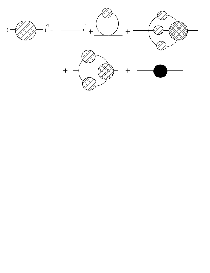
Figure 2: Schwinger - Dyson equation for the full propagator in $\lambda\phi^{4}$ theory. Symbols are the same as in Fig.1.

3 Super-Daisy approximation

The main problem of our method is how to approximate $\Pi$ in the Eq.(3). The function $\Pi$ is expressed by the full propagator, the full three and the full four point functions (Fig.1) according to the Schwinger - Dyson equation. The Schwinger - Dyson equation expresses the inverse of the full propagator by the relation expressed by Fig.2. In the right hand side of Fig.1, the first and the forth terms are independent of the external momentum and the second and the third terms depend on them. In this paper we assume the simplest case that the momentum independent term (the first term in Fig.1) is dominant. This corresponds to the well-known super-daisy approximation[7] which sums up all the graphs like Fig.3. We stress that the effective potential consists of all the super-daisy diagrams without over counting by this approximation.

\begin{picture}(16.0,6.5)\centerline{\hbox{ \epsfbox{figure3.eps} }} \end{picture}

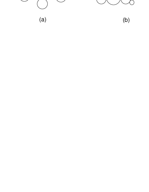
Figure 3: Examples of super-daisy diagrams. The graph (a) is often called merely a daisy diagram.

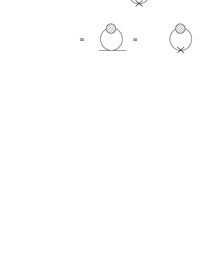
Figure 4: The relation between the self energy $\Pi$ and the derivative of the effective potential $V$ with respect to the mass square. See the first two term of Eq.(3).

In this approximation we see the following relation(Fig.4),

$$\Pi=\lambda(\frac{\partial V}{\partial m^{2}}-\frac{1}{2}{\bar{\phi}^{2}}).$$ (4)

In the following we ignore the third and forth terms in Eq.$(\ref{evo})$, considering that only the first two terms are important to discuss the phase transition[22]. Due to this approximation, we neglect the loop contribution remaining finite at $T=0$. Using relation (4) and integrating Eq.(3) over $p_{0}$ [10, 11, 24], we obtain the approximate evolution equation,

$$\frac{\partial V}{\partial m^{2}}=\frac{1}{2}\bar{\phi}^{2}+\frac{1}{2\pi^{2}}\int^{\infty}_{0}dp\frac{p^{2}}{\displaystyle 2\sqrt{p^{2}+m^{2}+\lambda\frac{\partial V}{\partial m^{2}}}}\frac{1}{\displaystyle\exp\left(\frac{1}{T}\sqrt{p^{2}+m^{2}+\lambda\frac{\partial V}{\partial m^{2}}}\right)-1}.$$ (5)

4 Numerical result

In the previous section we have obtained the evolution equation for $\frac{\partial V}{\partial m^{2}}$ under the super-daisy approximation. In this section we explain details of the numerical calculation and show its result.

4.1 Details of the numerical calculation

We can calculate the effective potential, by solving the Eq. (5) and integrating it according to the Eq. (1) numerically.

In the Eq. (1) we set the initial scale $m_{0}$ as large as $T$ so that we can evaluate the effective potential very well by the loop expansion. We use the same initial condition as was used in the previous paper[22],

$$V(m^{2}=m_{0}^{2}) = \frac{1}{2}m_{0}^{2}\bar{\phi}^{2}+\frac{\lambda}{4!}\bar{\phi}^{4}+\frac{T^{2}}{2\pi^{2}}\int^{\infty}_{0}dpp^{2}\log\left[1-\exp\left(-\frac{1}{T}\sqrt{p^{2}+m_{0}^{2}+\frac{\lambda}{2}\bar{\phi}^{2}}\right)\right].$$

The integral in the evolution Eq. (5) is well defined when the effective mass square, $m^{2}+\lambda\frac{\partial V}{\partial m^{2}}$, is real and positive. Below the critical temperature, however, the effective mass square can be negative or complex. We needs analytic continuation of the integral of the Eq.(5). This can be done by rewriting the Eq.(5) as in the previous paper[22],

$$\frac{\partial V}{\partial m^{2}}=\frac{1}{2}\bar{\phi}^{2}+\frac{T^{2}}{4\pi^{2}}\int^{\infty}_{0}dz\frac{\sqrt{z(z+2M)}}{e^{z+M}-1},$$ (7)

where $M={1\over T}\sqrt{m^{2}+\lambda\frac{\partial V}{\partial m^{2}}}$. To find $\partial V/\partial m^{2}$ we solve Eq.(7).

As is well-known, the effective potential becomes complex at small ${\bar{\phi}}$ below the critical temperature. It indicates instability of the state and the imaginary part of the effective potential is interpreted to be related with a decay rate of the state[23]. The imaginary part arises from the integral of the evolution equation in our method (see Eq.(7)). It is natural to suppose that the imaginary part of the effective potential is negative to interpret it with decay rate. In order that the imaginary part of the effective potential be negative, the imaginary part of $\frac{\partial V}{\partial m^{2}}$ must be positive(see Eq.(1)). We find that there are two solutions for the Eq. (7) and that their imaginary part has the opposite sign. We choose the solution of $\frac{\partial V}{\partial m^{2}}$ with positive imaginary part.

4.2 Result

Figure 5: Real part of the effective potential at $T=\mu t$. We see a small barrier to indicate a first order phase transition.

Figure 6: The field expectation value near the critical temperature at the stable point. We see a finite jump of $\bar{\phi}/\mu$ at $t=4.93\mu$ to indicate a first order phase transition.

Figure 7: Imaginary part of the effective potential at $T=\mu t$. We see the smaller $\bar{\phi}/\mu$ is, the larger the imaginary part is.

Let us explain the numerical result. For the graphs Fig.$(\ref{fig5})\sim(\ref{fig7})$ we set the four-point coupling $\lambda=1$.

We show the real part of the effective potential near the critical temperature in Fig.5. We see a small barrier between the symmetric vacuum ($\bar{\phi}=0$) and the symmetry-broken vacuum ($\bar{\phi}\neq 0$),which clearly shows a first order phase transition to occur.

A first order phase transition is also indicated by the behaviour of the field expectation value at the stable point, since Fig.6 shows there is a finite jump of it.

We get the negative imaginary part of the effective potential below the critical temperature and show it in Fig.7. We can see that the magnitude of the imaginary part increases as the field expectation value decreases. It expresses that the closer the field expectation value to the origin is, the less stable the state below the critical temperature is.

In the above we used the initial condition at $m=m_{0}=T$. It is required $m_{0}$ be the same order as the temperature in order that the initial condition can be evaluated by the perturbation. We have calculated the effective potential with other initial conditions $m_{0}=2T$ and $\frac{T}{2}$ and do not have found any appreciable change of the effective potential. It ensures the consistency of our calculation.

5 Summary and discussion

In this paper we have given a new method to calculate the effective potential of $\lambda\phi^{4}$ theory under the super-daisy approximation without over counting. We have numerically evaluated a real part and a imaginary part of the effective potential without using high temperature expansion. The real part indicates a first order phase transition though the true order should be second. The imaginary part indicates the instability is larger for the smaller expectation value of the field below the critical temperature.

\begin{picture}(16.0,4.0)\centerline{\hbox{ \epsfbox{figure8.eps} }} \end{picture}

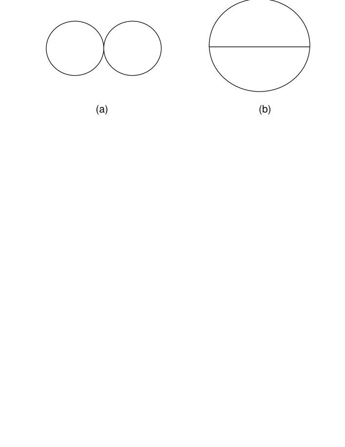
Figure 8: Two loop diagrams that contribute to the effective potential. (a) is daisy-like and (b) is not daisy-like.

Now we compare our method with other approaches. First we compare it with CJT method[17] which can also gather up the super-daisy graphs without over counting. It carried out by truncating the CJT expansion at $O(\lambda)$. A first order phase transition is indicated by the calculation of this model with this method as well as the high temperature expansion[19].

Second we compare with daisy-improved perturbation theory. In this method the effective potential indicates a first order phase transition at one loop level[13]. There are two graphs at two loop level(see Fig.8). If one includes the contribution of Fig.8(a) alone[13], the phase transition is still of first order. A second order phase transition is indicated when the contributions of both Fig.8(a) and Fig.8(b) are included. This indicates that the contribution of Fig.8(b), which is not daisy-like, seems to play the important role to the effective potential.

Finally we compare our result with the approximation of the previous paper. In the previous paper we get the effective potential that indicates a second order phase transition. The contributions of the second and the third terms of Fig.1 with zero external momentum are taken into account by the previous approximation. The difference of the two approximations is whether we include the contributions of the daisy-like diagrams only or not. This also indicates that non-daisy-like diagrams are important for the second order phase transition to be derived correctly.

According to the above comparisons, the diagrams which are not daisy like seem to give important contributions. We have to take into account the contribution of the second and the third terms in Fig.1. Their momentum dependence, especially the dependence on the small momentum, will be important in Eq.(3) since the infrared behaviour of the self energy plays a very important role for a second order phase transition[25]. This method with $\frac{\partial V}{\partial m^{2}}$ seems attractive because it may bring a chance to step in the region where the perturbation theory breaks down.

We finally express our thanks to A. Niegawa and T. Inagaki for valuable discussions and communications.

References

- [1] D.A.Kirzhnits and A.D.Linde, Phys. Lett. B42 (1972) 471.
- [2] V.Kuzmin, V.Rubakov and M.E.Shaposhnikov, Phys. Lett. B155 (1985) 36.
- [3] P.Arnold and O.Espinosa, Phys. Rev. D47 (1993) 3546.
- [4] Particle Deta Group, Phys. Rev. D54 (1996) 1.
- [5] M.E.Shaposhnikov, hep-ph/9610247.
- [6] P.Arnold, Proceedings of Quarks ’94 (1994) 71 (hep-ph/9410294).
-
[7]
L.Dolan and R.Jackiw,
Phys. Rev. D9 (1974) 3320;
- [8] S.Weinberg, Phys. Rev. D9 (1974) 3357.
- [9] P.Fendley, Phys. Lett. B196 (1987) 175.
- [10] J.I.Kapusta, “Finite Temperature Field Theory” Cambridge
- [11] M.Le.Bellac, “Thermal Field Theory”Cambridge.
- [12] M.E.Carrington, Phys. Rev. D45 (1992) 2933.
- [13] K.Takahashi Z.Phys.C26 (1985) 601.
- [14] J.M.Peskin and D.V.Schroeder, ”An Introduction to Quantum Field Theory” Addison Wesley.
- [15] K.Kajantie, M.Laine, K.Rummukainen and M.E.Shaposhnikov, Phys. Rev. Lett. 77 (1996) 2887, hep-lat/9612006.
- [16] P.Arnold and L.G.Yaffe, Phys. Rev. D49 (1994) 3003.
- [17] J.Cornwall, R.Jackiw, and E.Tomboulis, Phys. Rev. D10 (1974) 2428.
- [18] G.Amelino-Camelia, Phys. Rev. D49 (1994) 2740.
- [19] G.Amelino-Camelia and S.Y.Pi, Phys. Rev. D47 (1993) 2356.
- [20] K. Farakos, K. Kajantie, K. Rummukainen, M.Shaposhnikov Nucl.Phys. B425 (1994) 67.
- [21] W.Buchmüller and O.Phlipsen Nucl.Phys. B443 (1995) 47.
- [22] T.Inagaki, K.Ogure and J.Sato, hep-th/9705133.
- [23] E.Weinberg and A.Wu , Phys. Rev. D36 (1987) 2474.
- [24] P.D.Morley and M.B.Kislinger, Phys.Rep.51 (1979) 63.
- [25] K. G. Wilson and J. Kogut, Phys.Rep. 12C (1974) 75.