Novel field theory phenomena from F theory and D-branes

Abstract

Talk presented in the 97 Karpatcz winter school. We describe Sen’s work on F theory on K3 and its reflection on the world-volume field theory on a D3-brane probe. Field theories on a multiple of probes are analyzed. We construct a 4d N=1 superconformal probe theory which is invariant under electric-magnetic duality via a compactification to six dimensions on ${\bf T}^{6}/{\bf Z}_{2}\times{\bf Z}_{2}$.

1 Introduction

Recent developments in string theories, and in particular brane physcis, have provided new magnifying glasses for observations on quantum field theories in various dimensions. In this series of talks presented in the Karpatcz 97 winter school we have focused on exploring field theories on the world-volume of D-brane probes in F theory[2]. We have followed the analysis of A. Sen[3] on F theory on K3 and its reinterpretation in terms of a probe theory[5].

General background on D-branes, type $II_{B}$ theory, orientifolds and F theory is presented in the introduction section. Section 2 is devoted to the analysis of F theory compactified on K3[3] and its relation to the field theory on a D3-brane probe[BDS]. A generalization of the latter to the theory on a multiple probe system that is put in various configurations with respect to the orientifold plane[6] is presented in section 3. Section 4 is devoted to the extraction of the properties of a probe theory in the neighbourhood of an intersecting orietifold planes of an F compactified on ${\bf T}^{6}/{\bf Z}_{2}\times{\bf Z}_{2}$. The field content is found using a Gimon-Polchinski[4] type of analysis and a superpotential of this $N=1$ theory, which admits a fixed line passing through the origin of the space of couplings, is written down. The last 2 sections are based on a work that was done in collaboration with O. Aharony, S. Theisen and S. Yankielowicz[6],

1.1 A brief review of D-branes

A Dp-brane is a p dimensional extended object prescribed by the property that ends of open strings can lie on it, although open strings cannot exist in the bulk.[7] These open strings have Neuman boundary conditions (b.c) $\partial_{n}X^{\mu}=0$ for $\mu=0,1,...,p$ and Dirichlet b.c $X^{\mu}=constant$ for $\mu=p+1,...9$.

We summarize several properties of D-branes that we will make use of [8]: (i) The D-brane is a dynamical object. It can fluctuate in transverse directions. Its world-volume theory includes gauge fields and scalar fields. The latter correspond to the fluctuations. (ii) A Dp-brane couples to a $A_{p+1}$ form. Thus type $II_{A}$ includes even branes and $II_{B}$ odd ones. (iii) A T-duality on $S^{1}$ interchanges the Dirichlet and Neuman b.c on the $S^{1}$, so that a wrapped Dp-brane $\rightarrow$ D(p-1)-brane and unwrapped Dp-brane $\rightarrow$ D(p+1)-brane. (iv) a D-brane is a BPS state. It breaks half of the supersymmetries. (v) There is no force between infinite parallel D-branes at rest. (vi) N parallel D-branes can form a bound state at threshold.

1.2 A. brief review of type $II_{B}$ string theory

We briefly summarize the bosonic fields and the symmetries of type $II_{B}$ string theory.

1. Massless bosonic fields:

   Neveu-Schwarz (NS-NS) sector- $\phi$,  $g_{\mu\nu}$, $B^{(NS)}_{\mu\nu}$.

   Ramond-Ramond (RR) sector- $a$,  $B^{(RR)}_{\mu\nu}$, $D^{+}_{\mu\nu\rho\sigma}$

2. Symmetries

   I. Symmetries of the perturbative theory-

   (i) $(-1)^{F_{L}}$

   $a\rightarrow-a$; $B^{(RR)}_{\mu\nu}\rightarrow-B^{(RR)}_{\mu\nu}$; $D^{+}_{\mu\nu\rho\sigma}\rightarrow-D^{+}_{\mu\nu\rho\sigma}$

   (ii) $\Omega$ world sheet parity transformation-

   $a\rightarrow-a$; $B^{(NS)}_{\mu\nu}\rightarrow-B^{(NS)}_{\mu\nu}$; $D^{+}_{\mu\nu\rho\sigma}\rightarrow-D^{+}_{\mu\nu\rho\sigma}$

   II. conjectured non-perturbative symmetry

   $SL(2,{\cal Z})$S-duality-

   $$\framebox{$\displaystyle{\lambda}\rightarrow{p{\lambda}+q\over r{\lambda}+s}\ \ \left(\matrix{{B^{(NS)}_{\mu\nu}\ }\cr{B^{(RR)}_{\mu\nu}\ }\cr}\right)\rightarrow\left(\matrix{{p\ }{q\ }\cr{r\ }{s\ }\cr}\right)\left(\matrix{{B^{(NS)}_{\mu\nu}}\cr{B^{(RR)}_{\mu\nu}\ }\cr}\right)$}$$

   where

   $${\lambda}=a+ie^{-\phi}$$

   $p,q,r,s\in{\cal Z}$ with $ps-qr=1.$

1.3 A brief review of type $II_{B}$ orientifolds

Type $II_{B}$ defined on ${{\cal M}\over G}$ where ${\cal M}$-manifold and $G$- a group containing at least one element of the form

$$g_{s-t}\cdot g_{int}\cdot\Omega$$

where $g_{s-t}$ is a space-time transformation, $g_{int}$- is an internal transformation and $\Omega$ is a world-sheet parity transformation.

Here are some examples of type $II_{B}$ orientiflods

1. type $II_{B}$ on ${M^{9,1}\over\{1,\Omega\}}$ This is type I string theory on $M^{9,1}$.

2. type $II_{B}$ on $M^{7,1}\times{T^{2}\over{\cal I}_{89}(-1)^{F_{L}}\Omega}$ ${\cal I}_{89}$ transforms $x^{8}\rightarrow-x^{8}\ \ \ x^{9}\rightarrow-x^{9}$

   Upon performing T-duality on $T^{2}$ this is type I on $M^{7,1}\times T^{2}$.

3. type $II_{B}$ on $M^{5,1}\times{T^{4}\over({\cal I}_{67}(-1)^{F_{L}}\Omega)\times{\cal I}_{89}(-1)^{F_{L}}\Omega)}$

1.4 A brief review of F theory 

In conventional compactifications of type $II_{B}$ ${\lambda}=constant$.

F theory is defined in the following way. Let ${\cal M}$ be a manifold of dimension $d+2$ admitting an elliptic fibration. Let ${\cal B}$ be a (base) manifold of dimension d. ${\cal M}$ is obtained by erecting at every point of ${\cal B}$ a copy of a torus $T^{2}$ with its complex structure varying over ${\cal B}$.

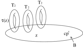
Figure 1:

F theory on $${\cal M} \equiv II_{B} {\cal B}$$  type  on

with

$${\lambda}=\tau(z)\neq\ constant$$

Note that when one moves along a closed cycle ${\lambda}=\tau(z)$ must come to its orignal value up to an $SL(2,{\cal Z})$transformation. An example of elliptic fibration- elliptically fibered $K3$. In this case ${\cal M}$- $K3$ and ${\cal B}$-$CP^{1}$. For $z$ the coordinate of $CP^{1}$ the torus is parametrized by the complex coordinates $x$ and $y$

$$y^{2}=x^{3}+f_{8}(z)x+g_{12}(z)$$ (1)

$f_{8}(z)$ and $g_{12}(z)$ are polynomials of degree 8 and 12 respectively.

The $J$ invariant of $T^{2}$ is given by

$$j(\tau(z))={4(24f)^{3}\over 27g^{2}+4f^{3}}$$ (2)

F theory on $K3$ is equivalent to type $II_{B}$ on $CP^{1}$ with ${\lambda}={\tau}(z)$. We enlist here several Dualities of F theory  that will be useful in the discussions below.

1. F theory on ${T^{2}\over Z_{2}}$  $\Leftrightarrow$  type I (heterotic) $SO(32)$

2. F theory on ${\cal M}\times S_{1}$$\Leftrightarrow$type $II_{B}$ on ${\cal B}\times S_{1}$ with ${\lambda}(z)={\tau}(z)$ of the fibers. Recall that type $II_{B}$ on $S_{1}$ with radius $R$ is dual to type $II_{A}$ on on $S_{1}$ with radius ${1\over R}$. Furthermore, type $II_{A}$ on $S_{1}$ is equivalent to M-theory on $T^{2}$, so that ${\lambda}$ of the type $II_{B}$ theory is identified with ${\tau}$ of the latter $T^{2}$. We thus conclude that

   F theory on $${\cal M}\times S_{1} \Leftrightarrow {\cal M}$$M-theory on

3. From (1) F theory on $K3\times S_{1}$$\Leftrightarrow$M-theory on $K3$$\Leftrightarrow$Heterotic on $T^{3}$.

   In a similar manner, F theory on $K3$$\Leftrightarrow$Heterotic on $T^{2}$.

   Since the heterotic theory on $T^{2}$$\Leftrightarrow$type $I$ on $T^{2}$$\Leftrightarrow$type $II_{B}$ on ${T^{2}\over{\cal I}_{89}}$ one finds

   F theory on $$K3 \Leftrightarrow II_{B} {T^{2}\over{\cal I}_{89}}$$type  on

4. F theory on K3 fibered CY $\Leftrightarrow$heterotic on K3.

2 Sen’s model- F-theory on K3- space-time and worldvolume theories

Eliptic fibration of K3 is described by eqn. (1). The idea of Sen was to look for a point in the F-theory moduli space where

$\tau(z)$ is independent of $z$ and $Im(\tau)$ is large

This should imply a conventional perturbative string compactification, and as will be shown below a conformal invariant field theory on a “probe” worldvolume.

A constant $\tau(z)$ means also

$$j(\tau(z))=constant\rightarrow{f^{3}\over g^{2}}=constant$$ (3)

This condition is obeyed if one takes

$$f=\alpha\phi(z)^{2},\ \ \ g=\phi(z)^{3}$$ (4)

In that case $j(\tau(z))={4(24\alpha)^{3}\over 27+4\alpha^{3}}=constant$ where $\alpha$ can be adjusted so that $Im(\tau)$ is large.

Singularities of $j(\tau)$ at

$$\Delta=(27g^{2}+4f^{3})=0$$ (5)

For the ansatz (4) and with $\phi\sim\prod_{i=1}^{4}(z-z_{i})$

$$\Delta\sim\prod_{i=1}^{4}(z-z_{i})^{6}$$ (6)

Metric on the base $CP^{1}$

In general the metric is given by[11]

$$ds^{2}=F(\tau,\bar{\tau}))\prod_{i=1}^{24}(z-z_{i})^{-{1\over 12}}\prod_{i=1}^{24}(\bar{z}-\bar{z}_{i})^{-{1\over 12}}$$

So for the point in moduli space we consider it takes the form

$$\framebox{$\displaystyle ds^{2}=F(\tau,\bar{\tau}))\prod_{i=1}^{4}(z-z_{i})^{-{1\over 2}}\prod_{i=1}^{4}(\bar{z}-\bar{z}_{i})^{-{1\over 2}}$}$$

This can be brought to the form of a Flat metric. Define

$$dw=\prod_{i=1}^{4}(z-z_{i})^{-{1\over 2}}dz$$

then

$$ds^{2}=dwd\bar{w}.$$

Near $z=z_{i}$,   $w\sim(z-z_{i})^{-{1\over 2}}$, namely, there is aConical deficit angle of $\pi$ at each of the four $z_{i}$.

Naively, we may conclude that

$${\cal B}={T^{2}\over{\cal I}_{89}}$$ (7)

But there is a subtlety, lets check again

$$\framebox{$\displaystyle y^{2}=x^{3}+\alpha x\prod_{i=1}^{4}(z-z_{i})^{2}+\prod_{i=1}^{4}(z-z_{i})^{3}$}$$ (8)

going around an orbifold point like $z=z_{i}$

$$(z-z_{i})\rightarrow e^{2\pi i}(z-z_{i})$$

$$x\rightarrow e^{2\pi i}x=x$$

$$y\rightarrow e^{3\pi i}y=-y$$

which is

$$An\ \ trans.\pmatrix{-1&\cr&-1\cr}\ on\ the\ T^{2}fiber$$SL(2,Z)

The transformation $\pmatrix{-1&\cr&-1\cr}$ corresponds to

$$(-1)^{F_{L}}\Omega$$

Thus, the the base is infact an Orientifold

$${\cal B}={T^{2}\over(-1)^{F_{L}}{\cal I}_{89}\Omega}.$$

Under this projection $z\rightarrow-z$, so define $u=z^{2}$ which is single valued on the orientifold.

The orientifold

(1) preserves half of the space-time supersymmetries of type $II_{B}$ .

(2) It carries a RR topological charge $-4$[7]

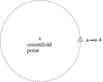
Figure 2:

$$\oint_{C}da=-4$$ (9)

where $C$ is a contour around $u=0$

D7-brane

(1) preserves half of the space-time supersymmetries of type $II_{B}$ .

(2) It carries a RR topological charge $+1$

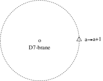
Figure 3:

To cancell the RR charges of the 4 orientifolds the theory must have 16 D7-branes see fig. 4.

Since we have a configuration with

$\lambda=constant\rightarrow a=constant$ the RR charge must be cancelled locally on the orientifold (fig. 5)

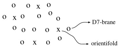
Figure 4:

There is an Enhanced symmetry at singularies that can be viewed in F-theory picture and in the orientifold picture.

Start with F-theory picture

$$y^{2}=x^{3}+\alpha x\prod_{i=1}^{4}(z-z_{i})^{2}+\prod_{i=1}^{4}(z-z_{i})^{3}$$ (10)

Near $z=z_{1}$

$$\tilde{y}^{2}=\tilde{x}^{3}+\alpha\tilde{x}(z-z_{1})^{2}+(z-z_{1})^{3}$$ (11)

which means that there is a

$$D_{4} \rightarrow\ SO(8)^{4}$$ type singularity  gauge symmetry

Now the orientifold description Let us construct the string configuration in several steps: (i) From strings starting and ending on the 7Dbrane fig. 6. one finds

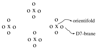
Figure 5:

$N=1$ 8D wv theory with $U(1)$ gauge field and a complex scalar that corresponds to the location of the D-brane in the $z$ plane.

(ii) When two D-branes collapse one gets (fig. 7)

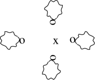
Figure 6:

$N=1$ 8D wv theory with $U(2)$ gauge fields and a complex scalar in the adjoint.

(iii) When all the four $z_{i}$ are equal (fig. 8) then the

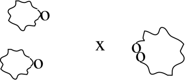
Figure 7:

symmetry is enhanced to $U(4)$

(iv) when all the four $z_{i}=0$ (fig. 9)

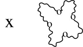
Figure 8:

there are additional strings (and hence massless vectors) between the 7branes at $z_{i}$ and their mirrors at $-z_{i}$. Now the symmetry is enhanced to $U(8)$

(v) But the generator of $Z_{2}=(-1)^{F_{L}}{\cal I}_{89}\Omega$ acts on the generators $T^{a}$ of the $U(8)$.

Only those that commute with it survive. Under $Z_{2}$

$$\framebox{$\displaystyle T^{a}\rightarrow_{Z_{2}}-\pmatrix{0\ I_{4}\ \cr I_{4}\ 0\ \cr}\ (T^{a})^{T}\ \pmatrix{0\ I_{4}\ \cr I_{4}\ 0\ \cr}$}$$

the various factors of this transformations are (i)-sign: change the sign of the oscillator $A^{\mu}_{-1}$ that creates open strings from the vaccum.

(ii)Tranaspose: effect of orientation reversal

(iii)$\pmatrix{0I_{4}\cr I_{4}0\cr}$ : effect of exchange of Dbranes and their images. This breaks

$$U(8)\rightarrow SO(8)$$

Let us now move away from the special point in the moduli space by switching background fields in both the orientifold and F-theory descriptions.

Deforming away from the special point-

Orientifold description- At each of the orientifolds the 7D-branes can be moved away from the orientfold. Near one particular orientifold the theory is type $II_{B}$ on ${{\cal R}^{2}\over(-1)^{F_{L}}{\cal I}_{89}\Omega}$ and the picture is like that of the neighborhood of a D7-brane in fig. 5.

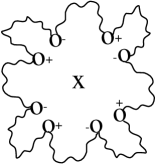
Figure 9:

The background field $\lambda$

$$\framebox{$\displaystyle{\lambda}(z)={\lambda}_{0}+{1\over 2\pi i}(\sum_{i=1}^{4}\ln(z-z_{i})-4\ln z)$}$$

It is clear that close to $z=0$ solution not consistent since $Im({\lambda})<0$.

F-theory description

Around the orbifold point

$$y^{2}=x^{3}+f(z)x+g(z)$$

where $f(z)$ and $g(z)$ are polynomial of degree 2 and degree 3 respectively.

The zeros of $\Delta$ are now at 6 singular points

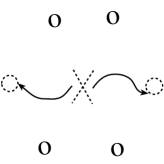
Figure 10:

The total number of parameters is

$$3\ from\ (f)+4\ from\ (g)$$

$$-1from\ rescaling\ of\ x,y\ -1shift\ of\ z=5$$

Recall the Seiberg-Witten solution for $N=2$ $SU(2)$ gauge symemtry with $N_{f}=4$ is parametrized by

$$\tau(z,\ \ m_{1},\ \ m_{2},\ \ m_{3},\ \ m_{4},\ \ \tau_{0})$$

where $z=<\phi^{2}>$, $m_{i}$ are quark masses and $\tau_{0}$ is the classical coupling. It is now natural to use the SW parameters $z,\tau_{0},m_{i}$ to label the F-theory background.

In this description the singularities are associated with massless quarks, massless monopole and massless dyon.

	orientifold	F-theory
para-	${\lambda}_{0},$	${\tau}_{0},$
meters	$z_{1},z_{2},z_{3},z_{4}$	$m_{1},m_{2},m_{3},m_{4}$
back-	${\lambda}(z)=$	${\lambda}(z)=$
	${\lambda}_{0}+{1\over 2\pi i}(\sum_{i=1}^{4}$	${\tau}({\tau}_{0},m_{i})$
ground ${\lambda}$	$\ln(z-z_{i})-4\ln z)$
asymp-	${\lambda}_{0}$	${\tau}_{0}$
totic ${\lambda}$
BPS	$z_{i}$	$m_{i}^{2}$
spectrum

The orientifold solution for ${\lambda}(z)$ is the same as the SW solution for large $z$ ($u$)

$${\tau}(z)={\tau}_{0}+{1\over 2\pi i}(\sum_{i=1}^{4}\ln(z-m_{i}^{2})-4\ln z)$$

The singularities $\ln(z-m_{i}^{2})$ are due to the masselss quarks and the $4\ln z$ term is associated with massless $SU(2)$ gauge bosons which splits into two singularities in the full solution. The comparison between the orientifold and the F theory picture is summarized in the table above.

We can now conclude that    F-theory provides the quantum corrected version of the orientifold background in the form of Seiberg-Witten solution   

Question:

Is it a conincidence that the SW theory emmerged?

2.1 SW solution as the wv theory on a 3B probe

Let us study the effective Lagrangian on a probe that moves in the background of the F-theory on K3.

Question: What probe should one use? 3Brane is the most natural probe since: (1) 3Brane is invariant under $SL(2,{\cal Z})$, so the wv theory should also be invariant under $SL(2,{\cal Z})$duality, (2) 7Brane parallel to a 3Brane probe breaks $1/2$ of the supersymmetries so that $\rightarrow$ $N=2$ in 4D.

Another interpretation of the 3Brane probe is as a wrapped 5Brane. Recall F-theory on K3 is dual to type I on $T^{2}$. Take a 5Brane of type I. Perform a T-duality on the $T^{2}$ which interchanges $N$$\Leftrightarrow$$D$ boundary conditions, and you find a 3D-Brane of type I’. The Chan-Paton $SU(2)$ gauge group of the 5Brane of type I is inherited by the 3Brane of the type I’. The comparison between the two dual pictures is summarized in the following table[5].

type I 5Brane	type I’ 3Brane
Wilson lines	3Brane position
around cycles	on ${T^{2}\over Z_{2}}$ away
of $T^{2}$	from orientifold
$SU(2)\rightarrow U(1)$	$SU(2)\rightarrow U(1)$
position of 7Brane	position of 7Brane
$R^{\prime}_{8}\alpha_{i,8}+iR^{\prime}_{9}\alpha_{i,9}$	$m_{i}$
position of 3Brane	position of 3Brane
$R^{\prime}_{8}A_{8}+iR^{\prime}_{9}A_{9}=\pmatrix{w&0\cr 0&-w}$	$z=w^{2}$

where the notation in this table is that of ref. [5]. The strings streched from the 3Brane to the 7Brane induce fundamental matter hypers with mass $m_{i}\pm w$.

Let us summarize the correspondence between the F theory and the probe theory:

(i) The set-up on the 3Brane wv is that of $SU(2)$ SW theory with four hyper-multiplets in the fundamental rep.

(ii) The F-theory ${\lambda}$ $\rightarrow$  probe gauge coupling ${\tau}$.

(iii) The fact that ${\lambda}=constant$   $\rightarrow$   into confomal invarinace of the probe theory.

(iv) type $II_{B}$ $SL(2,{\cal Z})$invarinace  $\rightarrow$ $SL(2,{\cal Z})$invariace of $SU(2)$ with $N_{f}=4$

3 The world-volume field theory on a multiple of 3-branes probes in 8 dimensions

Consider again F theory on K3. Recall that F theory on K3 is dual to type $I$ on $T^{2}$. Now wrap $N_{c}$ 5B around the $T^{2}$. Let us analyze the properties of a world-volume theory on the muptiple probes [15].

(i)Supersymmetry- 8 susy charges $N=1$ in 5+1 dim$\rightarrow$ $N=2$ in 3B 3+1 wv.

(ii)Gauge symmetry- $USP(2N_{c})$[9]

Hypermultiplets- (a) $A$- antisymmetric rep. $N_{c}(2N_{c}-1)$ which is irreducible $N_{c}(2N_{c}-1)$-1 $\oplus$ singlet.

(b) $N_{f}=4$ $Q^{i}$, “quarks” in the fundamental rep. $2N_{c}$ which emerge in F theory from strings between 3B and the four 7B at the orientifold point.

(iii)Global symmetry- $SO(8)$ global symmetry (local symmetry in space-time)

(iv)Superpotential- $W=Q^{i}XQ^{i}+AXA+m_{ij}Q^{i}Q^{j}$

(v)Mass terms- $m_{ij}$ corresponds to the complex scalar $28$ atisymmetric rep. of the space-time $SO(8)$ laocal sym. No other scalars in space-time$\rightarrow$ No mass term to $A$.

(vi)$\beta$ function $(2N_{c}+2)\ -(2N_{c}-2)\ -\ 4=0$

(vii)Expectation values- (a) scalars of the antisymmetric rep which correspond to the motion in $x_{4},x_{5},x_{6},x_{7}$. (b) scalars of vector multiplet associated with Wilson loops of the gauge fields around $T^{2}$.

(viii)Moduli space of Coulomb branch-

$${(SU(2)^{k})\over S_{k}}$$

parmutation symmetry $S_{k}$ part of the $USP(2N_{c})$ Weyl group.

3.1 Flows of the $USP(2N_{c})$ theory

(1) $USP(2N_{c})\ \rightarrow\ U(1)^{N_{c}}$

$$<X>=diag(a_{1},a_{2},\cdots,a_{k},-a_{1},-a_{2},\cdots,-a_{k})$$

where $a_{i}^{2}$ corresponds in the type $II_{B}$ picture to the localtion of the $i^{th}$ 3B on ${T^{2}\over Z_{2}}$ from the orientifold.

Figure 11:

(2) $USP(2N_{c})\ \rightarrow\ SU(2)^{N_{c}}$

$$<A>=\pmatrix{0&0&\cdots&0&b_{1}&0&\cdots&0\cr 0&0&\cdots&0&0&b_{2}&\cdots&0\cr\vdots&\vdots&\ddots&\vdots&\vdots&\vdots&\vdots&\vdots\cr 0&0&\cdots&0&0&0&\cdots&b_{k}\cr-b_{1}&0&\cdots&0&0&0&\cdots&0\cr 0&-b_{2}&\cdots&0&0&0&\cdots&0\cr\vdots&\vdots&\vdots&\vdots&\vdots&\vdots&\ddots&\vdots\cr 0&0&\cdots&-b_{k}&0&0&\cdots&0\cr}.$$

$b_{i}^{2}$ corresponds in the type $II_{B}$ picture to the localtion of the $i^{th}$ 3B in $x_{4},x_{5},x_{6}$ and $x_{7}$.

In the limit of all $b_{i}$ being very large only singlet remanants from $A$ survives so it flows to $N_{c}$ copies of Seiberg-Witten theory of $SU(2)$ with $N_{f}=4$.

(3) $USP(2N_{c})\ \rightarrow\ U({N_{c}});N=4$

The $N_{c}$ 3B are together but very far from the orientifold point [10].

Figure 12:

One can deduce from the probe theory interesting properties of the SW theories [6] To summarize:

The Coulomb phase of wv field theory of multiple $p$-branes is just $N_{c}$ copies (up to global identifications) of the Coulomb phase for a single $p$-brane.

4 Construction of $N=1$ superconformal 4D probe theory with electric-magnetic duality symmetry

Consider as in Sen’s model[3] compactifications of F- theory on CY manifolds which have a constant (weak coupling) value of $\tau$.

The simplest case is the elliptic fiber over a base ${\bf CP}^{1}\times{\bf CP}^{1}$[12] .

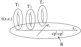
Figure 13:

In analogy to (1) the toric fibers are described by

$$y^{2}=x^{3}+f(z_{1},z_{2})x+g(z_{1},z_{2}),$$

where $z_{1}$ and $z_{2}$ label the two ${\bf CP}^{1}$s of the base.

$$\Delta=4f^{3}+27g^{2}=0$$

At a degeneration of the fibers, which is a location of type IIB 7-brane in the compact dimensions, $\tau$ has a non-trivial monodromy when going around it.

(i) in F-theory

$$\tau(z_{1},z_{2})=constant\rightarrow{f^{3}\over g^{2}}=constant$$

A solution (though not the most general solution) which generalizes (4) is

$$\framebox{$\displaystyle f(z_{1},z_{2})=\alpha\phi_{1}(z_{1})^{2}\phi_{2}(z_{2})^{2};\ g(z_{1},z_{2})=\phi_{1}(z_{1})^{3}\phi_{2}(z_{2})^{3},$}$$

where $\phi_{1}$ and $\phi_{2}$ are general polynomials of degree four

$$\framebox{$\displaystyle\phi_{1}(z_{1})=\prod_{i=1}^{4}(z_{1}-z^{(i)}_{1});\ \phi_{2}(z_{2})=\prod_{i=1}^{4}(z_{2}-z^{(i)}_{2}).$}$$

At this point in moduli space $\tau=constant(\alpha)$ and there are $D_{4}$ singularities at $z_{1}=z_{1}^{(i)}$ and at $z_{2}=z_{2}^{(i)}$.

4.1 Space-time theory at the intersection of the two $D_{4}$ singularities

In general the spacetime field theory at an intersection of two $D_{4}$ singularities is not well understood[13, 16]. Let us try to interpret this point in moduli space as an orientifold of the type IIB theory. Around each of the points $z_{1}=z^{(i)}_{1}$ (for constant $z_{2}$) there is an $SL(2,{\bf Z})$ monodromy of the form

$$\pmatrix{-1&0\cr 0&-1\cr}.$$

Locally, this monodromy can be interpreted as an orientifold of the type IIB theory by $(-1)^{F_{L}}\cdot\Omega$, accompanied by four 7-branes to cancel the RR charge.

Each point $z_{1}=z^{(i)}_{1}$ on the first ${\bf CP}^{1}$ factor carries a deficit angle of $\pi$, all four of them together deforming the two ${\bf CP}^{1}$ to ${\bf T}^{2}/{\bf Z}_{2}$. Thus, the theory looks like

$$\framebox{$\displaystyle type\ II_{B}\ on\ {{\bf T}^{4}\over{\bf Z}_{2}\times{\bf Z}_{2}^{\prime}}$}$$

where

$$z_{2}={\cal I}_{67}\Omega(-1)^{F_{L}};\ \ z_{2}^{\prime}={\cal I}_{89}\Omega(-1)^{F_{L}}.$$

Naively, this corresponds to the orientifold of F-theory on ${{\bf T}^{6}\over{\bf Z}_{2}\times{\bf Z}_{2}^{\prime}}$.

However, this orientifold compactification cannot be identified directly with the F-theory compactification[curve]

Generally, in F-theory compactification

$$B^{NS}_{\mu\nu}=B^{RR}_{\mu\nu}=0$$

In our case there is discrete non-vanishing $B_{\mu\nu}$fields (related to discrete torsion ) How do we know? At the intersection of two $D_{4}$ singularities the intersection point can be blown up to get an additional 2-cycle. In the naive F-theory compactification 3-brane can be wrapped over the vanishing 2-cycle, which should mean that there are $\Rightarrow$ tensionless strings living on the intersection of the $D_{4}$ singularities. Our orientifold construction, on the other hand, involves a well-defined weakly coupled conformal field theory, whose low-energy spectrum is well-defined and can not include such tensionless strings. Discrete ${\bf Z}_{2}$ symmetries force the value of both 2-form tensor fields (integrated over the vanishing 2-cycle) to be either $0$ or $1/2$ (modulo $1$).

A non-zero value for either (or both) of these fields breaks the $SL(2,{\bf Z})$ symmetry to a discrete $\Gamma(2)$ subgroup.

$$\Gamma(2);\{s=\pmatrix{\ 0&1\cr-1&0\cr},t^{2}=\pmatrix{\ 1&2\cr-0&1\cr}\}$$

There are two possible models:

(i) Integrated $B^{NS}={1\over 2},B^{RR}=0$ $\rightarrow$Sen’s $SU(4)$ model [14]

(ii) Integrated $B^{NS}=B^{RR}={1\over 2}$ $\rightarrow$ $SO(8)$ model[6]

4.2 The space-time theory of the $SO(8)$ model

The superfield content which one deduce from the various string sectors are given by:

(1)Untwisted closed string sectors :

supergravity multiplet $+$ one tensor multiplet $+$ 4 hypermultiplets.

Open string sector:

(i) 7-7 strings $\rightarrow$ $SO(8)^{4}$ vector multiplets.

(ii) 7’-7’ strings $\rightarrow$ $SO(8)^{4}$ vector multiplets.

(iii) 7-7’ no massless states.

(2) Twisted closed string sectors :

A tensor multiplet at each intersection of fixed points (i.e. at each fixed point of both ${\bf Z}_{2}$’s), accounting for a total of 16 additional tensor multiplets. At each intersection of $D_{4}$ singularities there is a possibility of blowing up a point to get an additional 2-cycle After all these blow-ups we get

F-theory on a smooth $(h_{11}=51,h_{21}=3)$ Calabi-Yau manifold.

which includes [17, 18, 19]:

$$n_{T}=h_{11}^{B}-1=18-1$$

$$n_{H^{0}}=h_{21}^{M}+1=3+1=4$$

$$r(V)=h_{11}^{M}-h_{11}^{B}-1=51-18-1=32$$

This set of 6D $N=1$ multiplets obey the anomaly cancellation condition

$$29n_{T}+n_{H}-n_{V}=293$$

Note again, that the spacetime theory we found (using the orientifold construction) is not the same as the theory we supposedly started with, which was F-theory compactified on an elliptic fibration over ${\bf CP}^{1}\times{\bf CP}^{1}$.

4.3 The space-time theory of the $SU(4)$ model

[14]

Untwisted closed string sectors :

supergravity multiplet $+$ one tensor multiplet $+$ 4 hypermultiplets.

Open string sector:

(i) 7-7 strings $\rightarrow$ $U(4)^{4}$ vector multiplets $+$ $2\times 6$ hypers for each vector.

(ii) 7’-7’ strings $\rightarrow$ $U(4)^{4}$ vector multiplets $+$ $2\times 6$ hypers for each vector.

(iii) 7-7’ $(4,4)$ hyper multiplets.

Twisted closed string sectors :

16 hypers

$$n_{T}=1,\ \ \ n_{H}=372\ n_{v}=128$$

4.4 3B probe wv field theory at the intersection

The probe theory is expected (i) to have only $N=1$ supersymmetry. ( since the 7-branes intersect transversely at this point and each breaks a different half of the wv $N=4$ supersymmetry,) (ii) to be invariant under conformal and ($\Gamma(2)$) electric-magnetic duality symmetry, and (iii) to have two deformations, corresponding to turning on $z_{1}$ or $z_{2}$, which should cause it to flow to the $N=2$ $SU(2)$ gauge theory with 4 quark hypermultiplets.

4.5 Fields from the 3-brane strings

Let us begin by computing the fields corresponding to strings which stretch out from a 3-brane and fold back to the same brane.

The 3-brane has 3 images under ${\bf Z}_{2}\times{\bf Z}_{2}$, so that every open string state is enhanced to a $4\times 4$ matrix (as in Gimon-Polchinski[4] (fig. 14 ) )

imposing the orientifold restrictions.

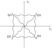
Figure 14:

The $\gamma$ matrices[4] corresponding to each of the generators in the ${\bf Z}_{2}\times{\bf Z}_{2}$ may be chosen to be

$$\gamma_{\Omega_{1}}=\pmatrix{0&i&0&0\cr-i&0&0&0\cr 0&0&0&i\cr 0&0&-i&0\cr}\gamma_{\Omega_{2}}=\pmatrix{0&0&i&0\cr 0&0&0&i\cr-i&0&0&0\cr 0&-i&0&0\cr}$$

and the orbifold matrix is then necessarily

$$\gamma_{T}=\gamma_{\Omega_{1}}\gamma_{\Omega_{2}}=\pmatrix{0&0&0&-1\cr 0&0&1&0\cr 0&1&0&0\cr-1&0&0&0\cr}.$$ (12)

These matrices are hermitian and unitary, and they correctly reflect the two ${\bf Z}_{2}$ actions on the compact coordinates $(z_{1},z_{2})$.

The wave-function matrices of states, $M_{ij}$, must then satisfy conditions of the type

$$M =\pm\gamma_{\Omega_{1}}M^{T}\gamma_{\Omega_{1}}^{-1}$$ (13)

$$M =\pm\gamma_{\Omega_{2}}M^{T}\gamma_{\Omega_{2}}^{-1}$$ (14)

$$M =\pm\gamma_{T}M\gamma_{T}^{-1}$$ (15)

where the signs are determined by the transformation properties of the relevant state.

For the gauge fields- $-,-,+$,

For the chiral superfield $X_{6,7}$ - $-,+,-$,

For $X_{8,9}$ - $+,-,-$

For $X_{4,5}$ - $+,+,+$.

Note that in flat space the 3-brane field theory involves an $N=4$ vector multiplet, containing an $N=1$ vector multiplet and three $N=1$ chiral multiplets corresponding to the coordinates $X_{4,5,6,7,8,9}$ of the 3-brane. In the presence of the orientifold, each of these fields is enhanced into a $4\times 4$ matrix with different constraints.

(i) Vector superfields

The relations imposed by (13) on the components $M_{ij}$ of gauge fields are

$$M_{11} =-M_{22}=-M_{33}=M_{44}$$ (17)

$$M_{14} =M_{41}=M_{23}=M_{32}$$ (18)

$$M_{12} =-M_{43}\quad M_{13}=-M_{42}$$ (19)

$$M_{21} =-M_{34}\quad M_{31}=-M_{24}.$$ (20)

A basis of 6 matrices that obey these relations is

$$Z_{1}=\pmatrix{1&0&0&0\cr 0&-1&0&0\cr 0&0&-1&0\cr 0&0&0&1\cr} Z_{2}=\pmatrix{0&0&0&-1\cr 0&0&-1&0\cr 0&-1&0&0\cr-1&0&0&0\cr}$$

$$W_{1}=\pmatrix{0&1&0&0\cr 1&0&0&0\cr 0&0&0&-1\cr 0&0&-1&0\cr} W_{2}=\pmatrix{0&0&1&0\cr 0&0&0&-1\cr 1&0&0&0\cr 0&-1&0&0\cr}$$

$$W_{3}=\pmatrix{0&0&i&0\cr 0&0&0&i\cr-i&0&0&0\cr 0&-i&0&0\cr} W_{4}=\pmatrix{0&i&0&0\cr-i&0&0&0\cr 0&0&0&i\cr 0&0&-i&0\cr}.$$

It is now straightforward to check that the matrices

$$W^{+}_{2}= {1\over 4}(W_{1}+W_{2});\ W^{-}_{1}={1\over 4}(W_{1}-W_{2});$$

$$\ W^{+}_{1}= {1\over 4}(W_{3}+W_{4});\ W^{-}_{2}={1\over 4}(W_{3}-W_{4})$$

$$Z^{\pm}= {1\over 4}(Z_{1}\pm Z_{2})$$

obey the following commutation relations

$$[Z^{+},W^{+}_{2}]= -iW^{+}_{1};\ \ [Z^{+},W^{+}_{1}]=iW^{+}_{2};$$

$$\ [W^{+}_{2},W^{+}_{1}]= -iZ^{+}$$

$$[Z^{-},W^{-}_{1}]= iW^{-}_{2};$$

$$\ [Z^{-},W^{-}_{2}]= -iW^{-}_{1};\ \ [W^{-}_{1},W^{-}_{2}]=iZ^{-}$$

$$[Z^{+},W^{-}_{1}]= 0;\ \ [Z^{+},W^{-}_{2}]=0;$$

$$\ [Z^{-},W^{+}_{2}]= 0;\ \ [Z^{-},W^{+}_{1}]=0;\ \ [Z^{+},Z^{-}]=0$$

$$[W^{+}_{2},W^{-}_{1}]= 0;\ \ [W^{+}_{2},W^{-}_{2}]=0;$$

$$\ [W^{+}_{1},W^{-}_{1}]= 0;\ \ [W^{+}_{1},W^{-}_{2}]=0.$$

Thus, we see that the gauge fields span an

$SU(2)\times SU(2)$ algebra.

Figure 15:

When we take $z_{1}$ to infinity all 1-2,1-4,2-3 and 3-4 strings become infinitely massive, (fig. 15) so we can drop those wave-function matrices with non-zero entries in those positions. This leaves $Z_{1},\,W_{2}$ and $W_{3}$, which generate an $SU(2)$ subalgebra.

Likewise, if we take $z_{2}$ to infinity. This picture is in accord with the naive expectation following Sen of having just a single $SU(2)$ near $z_{1}=0$ or $z_{2}=0$.

(ii) $X_{67}$ chiral multiplet

Next consider the implications of [mishgamma] on the scalar fields $X_{67}$. The constraints on the matrix components are now

$$M_{11} =-M_{22}=M_{33}=-M_{44}$$

$$M_{14} =-M_{41}=-M_{23}=M_{32}$$

$$M_{12} =+M_{43}\quad M_{13}=M_{42}=0$$

$$M_{21} =+M_{34}\quad M_{31}=M_{24}=0$$

A basis of hermitian matrices that obey the relations is the following

$$A_{1}=\pmatrix{1&0&0&0\cr 0&-1&0&0\cr 0&0&1&0\cr 0&0&0&-1\cr} A_{2}=\pmatrix{0&0&0&i\cr 0&0&-i&0\cr 0&i&0&0\cr-i&0&0&0\cr}$$

$$A_{3}=\pmatrix{0&1&0&0\cr 1&0&0&0\cr 0&0&0&1\cr 0&0&1&0\cr} A_{4}=\pmatrix{0&i&0&0\cr-i&0&0&0\cr 0&0&0&-i\cr 0&0&i&0\cr}.$$

Note that now if we take $z_{1}$ to infinity (naively) we are left only with $A_{1}$, while if we take $z_{2}$ to infinity (naively) we remain with $A_{1},A_{3}$ and $A_{4}$ which are in the adjoint representation of the remaining $SU(2)$, and thus we go over to the picture of Sen, as expected.

Define now the matrices

$A_{-+},A_{++},A_{--}$ and $A_{+-}$

by the equations

$A_{++}=A_{3}-iA_{4}$;  $A_{-+}=A_{1}+iA_{2}$; $A_{+-}=A_{1}-iA_{2}$ and $A_{--}=A_{3}+iA_{4}$.

It can easily be checked that

$A=(A_{++},A_{-+},A_{+-},A_{--})$ are in the

$(2,2)$ representation of $SU(2)\times SU(2)$ For instance, we have

$$[Z^{+},A_{++}]={1\over 2}A_{++}\ \ [Z^{+},A_{-+}]=-{1\over 2}A_{-+}$$

$$[W^{+}_{2},A_{++}]=-{1\over 2}A_{-+}\ \ [W^{+}_{2},A_{-+}]=-{1\over 2}A_{++}$$

$$[W^{+}_{1},A_{++}]={i\over 2}A_{-+}\ \ [W^{+}_{1},A_{-+}]=-{i\over 2}A_{++}$$

and so on.

(iii) $X_{89}$ chiral multiplet

For the relations on the $X_{89}$ chiral superfield we would find similar (but not identical) results to those of $X_{67}$ (with the second and third rows and columns of all matrices interchanged.)

Thus, this chiral superfield, that we denote by

$$B=(B_{++},B_{-+},B_{+-},B_{--})$$

, is also in the $(2,2)$ representation of $SU(2)\times SU(2)$

As a consistency check, we verify that a VEV for $X_{67}$, for instance, indeed breaks the gauge symmetry to a diagonal $SU(2)$. For instance, taking $A_{1}$ to have a VEV would leave exactly the matrices $Z_{1},W_{2}$ and $W_{3}$ (given above), which commute with it, as expected. The $A$’s would also all become massive except $A_{1}$ (since they do not commute with it), again as expected (since after moving along the flat direction we should have just a single scalar).

(iv) $X_{45}$ chiral multiplet

The relations for $X_{45}$ are

$$M_{11} =M_{22}=M_{33}=M_{44}$$

$$M_{14} =M_{41}=-M_{23}=-M_{32},$$

and their solutions are spanned by the two singlets $S_{1}$ and $S_{2}$

$$S_{1}=\pmatrix{1&0&0&0\cr 0&1&0&0\cr 0&0&1&0\cr 0&0&0&1\cr}\quad S_{2}=\pmatrix{0&0&0&1\cr 0&0&-1&0\cr 0&-1&0&0\cr 1&0&0&0\cr}$$

4.6 Fields form the strings between the 3-brane and 7-branes

The $\gamma_{\Omega}$ matrices for the 7-branes are all proportional to the identity matrix The constraint on the 7-brane gauge fields is then just

$$M=-M^{T},$$

giving an anti-symmetric matrix corresponding to an $SO(8)$ space-time gauge symmetry, since there are 8 7-branes when including the $Z_{2}$ partners.

Next, we should use these matrices to analyze the wave function of the 3-7 strings (as in [4]). The 7-brane side is trivial, so the orbifold/orientifold projections just mix the various 3-branes according to the $\gamma_{\Omega}$ matrices For instance taking the $3_{1}-7$ state (where $3_{1}$ is the first 3-brane) via $\gamma_{\Omega_{1}}$ to $i$ times the $7-3_{2}$ state (with opposite orientation !), via $\gamma_{\Omega_{2}}$ to $i$ times the $7-3_{3}$ state, and via $\gamma_{T}$ to minus the $3_{4}-7$ state. A basis for the states going to a specific 7-brane can thus be chosen to be

$$D^{+}_{u}=(1,0,0,-1);\qquad D^{+}_{d}(0,1,1,0).$$

Using the matrices we found above for the gauge fields, it is easy to check that these are doublets under $SU(2)_{+}$, and singlets with respect to $SU(2)_{-}$. The corresponding chiral superfields are thus in $(2,1)$ representation of $SU(2)_{+}\times SU(2)_{-}$. For the other group of 7-branes we can then do the same thing, but with minus the identity matrix for some of the relevant 7-7 $\gamma_{\Omega}$ matrices (say for $\gamma_{\Omega_{2}}$ and $\gamma_{T}$). Then, the basis comes out to be

$$D^{-}_{u}=(1,0,0,1);\qquad D^{-}_{d}(0,1,-1,0).$$

which is in the $(1,2)$ representation of $SU(2)_{+}\times SU(2)_{-}$.

The summary of the field content is

$A_{\mu}$— $SU(2)\times SU(2)$ gauge fields.

$X_{8,9}\equiv B$— chiral field in $(2,2)$    $A^{2}=z_{2}$

$X_{6,7}\equiv A$— chiral field in $(2,2)$    $A^{2}=z_{1}$

$X_{4,5}\equiv(S_{1},S_{2})$— singlet chiral fields

$Q^{i}$ ($i=1,\cdots,8$)—- chiral quarks in $(2,1)$

$q^{i}$ ($i=1,\cdots,8$)—- chiral quarks in $(1,2)$

Note about this particle spectrum.

(i) It is manifestly not $N=2$ supersymmetric (since there is no chiral multiplet in the adjoint representation)

(ii) $<A>\neq 0$ ($<B>\neq 0$) breaks $SU(2)\times SU(2)\rightarrow SU(2)$-

Three components of $A$ ($B$) are swallowed by the Higgs mechanism, and we remain with an adjoint chiral multiplet (coming from $B$ ($A$)) and additional singlets, as expected.

(iii) A natural interpretation of $S_{1}$ $S_{2}$ is that at the intersection point the 3-brane can split into two half-3-branes which can move independently.

(iv) Vanishing one loop $\beta$ function

(since there are 12 ($N_{f}=6$) doublets of each $SU(2)$).

4.7 The Superpotential

Let start with some general points:

(i) In principle, it should be possible to compute this superpotential from the string theory analysis, but we have not performed this computation.

(ii) Since we have only $N=1$ supersymmetry, the superpotential in general receives non-perturbative quantum corrections.

(iii) The superpotential has to obey the following main constraints:

1) The ($SO(8)$ theory should have (at least) an $SO(8)\times SO(8)$ global symmetry. The ($SU(4)$) theory should have (at least) an $SU(4)\times SU(4)$ global symmetry.

2) The theory should flow to the $N=2$, $SU(2)$, $N_{f}=4$ theory upon giving a VEV to $A$ or to $B$.

3) The theory should have a fixed line passing through weak coupling [20, 21].

4) The quarks $q^{i}$ ($Q^{i}$) have to become massive when we give a VEV to $A$ ($B$)

Construction of the superpotential:

(i) Superpotential for the quarks The vanishing of the $\beta$ function associated with the gauge coupling $\beta_{g}$ and with the superpotential couplings $\beta_{h_{n}}$ requires that

$$A_{g}= 3C_{2}(G)-\sum_{i}T(r_{i})+\sum_{i}T(r_{i})\gamma_{i}=0$$ (22)

$$A_{h_{n}}= (n-3)+{1\over 2}\sum_{k}\gamma_{k}=0$$ (23)

where in the first equation the sum is over all the fields in the theory, and in the second only over the fields in the particular term of the superpotential.

A fixed line passing through weak coupling demands that these equations are not all independent[20]. It is easy to check tht $n=3$ and $\gamma_{k}=0$ is a solution for this condition. In fact in [21] it was shown from string argumetns that indeed all the anomalous dimensions vanish.

Combining this solution with the requirements 1), 2) and 4) one ends up with the following superpotentials

For the $SU(4)$ model[14]

$$W=QA\tilde{Q}+qB\tilde{q}$$ (25)

and for the case of $SO(8)$[6]

$$W={QABQ\over{\sqrt{A^{2}}}}+{qABq\over{\sqrt{B^{2}}}}$$ (26)

Inspite of the fact that in both cases these superpotentials obey all the requirements, it is clear that only for the $SU(4)$ model it is an adequate solution. In the second case one encounters singularities in the limits of $A\rightarrow 0$ and $B\rightarrow 0$ which cannot be smoothed .

(ii) Construction of the superpotential for $S_{1},S_{2})$

(a) $S_{1}$- the location of the 3-brane in $X_{4,5}$ coordinates should be decoupled.

(b) $S_{2}$ (corresponding to splitting the 3-brane at the orientifold point) should be massless only when $A$ and $B$ are both zero.

(c) $A$ and $B$ become massive once $S_{2}$ is turned on, as expected, since when the 3-brane has split we cannot move it away from the orientifold point.

(d) In the “Coulomb branch” $<A^{2}>$ and $<B^{2}>$ should correspond to flat directions but not $AB$.

(e) $<A>$-three of its components are swallowed by the Higgs mechanism, and the other remains massless and parametrizes the flat direction corresponding to the flow (it is the $N=2$ partner of $S_{1}$). Three of the components of $B$ remain massless and become an adjoint field $X$ of the remaining $SU(2)$, but the remaining component, as well as $S_{2}$, should become massive (since we have no corresponding fields in the $N=2$ theory) The final result for this part of the action is

$$W=S_{2}AB$$

Acknowledgements We would like to thank A. Brandhuber, V. Kaplunovsky and especially A. Sen for useful conversations.

References

- [1]
- [2] C. Vafa, “Evidence for F-Theory”, Nucl. Phys. B469 (1996) 403, hep-th/9602022
- [3] A. Sen, “F Theory and Orientifolds”, Nucl. Phys. B475 (1996) 562, hep-th/9605150
- [4] E. G. Gimon and J. Polchinski, “Consistency Conditions for Orientifolds and D-Manifolds”, Phys. Rev. D54 (1996) 1667, hep-th/9601038
- [5] T. Banks, M. R. Douglas and N. Seiberg, “Probing F-Theory With Branes”, Phys. Lett. 387B (1996) 278, hep-th/9605199
- [6] O.Ahrony, J. Sonnenschein, S. Theisen and S. Yankielowicz “Field Theory Questions for String Theory Answers” hep-th9611222
- [7] J. Polchinski, “Dirichlet Branes and Ramond-Ramond Charges”, Phys. Rev. Lett. 75 (1995) 4724, hep-th/9510169
- [8] J. Polchinski, S. Choudhuri and C. Johnson, hep-th/9502052
- [9] E. Witten, “Small Instantons in String Theory”, Nucl. Phys. B460 (1996) 541, hep-th/9511030
- [10] E. Witten, “Bound States of Strings and -branes”, Nucl. Phys. B460 (1996) 335, hep-th/9510135
- [11] B. Greene, A. Shapere, C. Vafa and S. -T. Yau Nucl. Phys. B337 (() 1990) 1.
- [12] D. R. Morrison and C. Vafa, “Compactifications of F-Theory on Calabi-Yau Threefolds I,II”, Nucl. Phys. B473 (1996) 74, hep-th/9602114; Nucl. Phys. B476 (1996) 437, hep-th/9603161
- [13] M. Bershadsky, K. Intriligator, S. Kachru, D. R. Morrison, V. Sadov and C. Vafa, “Geometric Singularities and Enhanced Gauge Symmetries”, hep-th/9605200
- [14] A. sen “A Non-perturbative Description of the Gimon-Polchinski Orientifold”hep-th/9611186 Nucl. Phys. B489 (() 1997) 139; “ F-theory and the Gimon-Polchinski Orientifold” hep-th/9702061; “Orientifold Limit of F-theory Vacua” hep-th/9702165.
- [15] This topic was also discussed in: M. R. Douglas, D. A. Lowe and J. H. Schwarz “Probing F-theory With Multiple Branes” hep-th/9612062 Phys. Lett. 394B (1997) 297
- [16] M. Bershadsky and A. Johansen, “Colliding Singularities in F Theory and Phase Transitions”, hep-th/9610111
- [17] J. D. Blum and A. Zaffaroni, “An Orientifold from F-Theory”, Phys. Lett. 387B (1996) 71, hep-th/9607019
- [18] A. Dabholkar and J. Park, “A Note on Orientifolds and F-Theory”, hep-th/9607041
- [19] R. Gopakumar and S. Mukhi, “Orbifold and Orientifold Compactifications of F-Theory and M Theory to Six and Four Dimensions”, hep-th/9607057
- [20] R. G. Leigh and M. Strassler, “Exactly Marginal Operators and Duality in Four Dimensional Supersymmetric Gauge Theory”, Nucl. Phys. B447 (1995) 95, hep-th/9503121
- [21] O. Aharony, S. Kachru and E. Silverstein, “New superconformal field theories in four dimensions from D-brane probes”, hep-th/9610205