Non-perturbative approach to the effective potential of the $\lambda\phi^{4}$ theory at finite temperature

Tomohiro Inagakia, Kenzo Ogureb and Joe Satoc
a Department of Physics, Kobe University,
Rokkoudai, Nada, Kobe 657, Japan
b
Institute for Cosmic Ray Research, University of Tokyo,
Midori-cho, Tanashi, Tokyo 188-8502, Japan

c Department of Physics, University of Tokyo,
Bunkyo-ku, Hongo, Tokyo 133-0033, Japan
e-mail address: inagaki@hetsun1.phys.kobe-u.ac.jpe-mail address: ogure@icrr.u-tokyo.ac.jpe-mail address: joe@hep-th.phys.s.u-tokyo.ac.jp
Abstract

We construct a non-perturbative method to calculate the effective potential of the $\lambda\phi^{4}$ theory at finite temperature. We express the derivative of the effective potential with respect to the mass square in terms of the full propagator. We reduce it to the partial differential equation for the effective potential using an approximation. We numerically solve it and obtain the effective potential non-perturbatively. We find that the phase transition is second order as it should be. We determine several critical exponents.
PACS numbers: 05.70.Fh; 11.10.Wx; 11.15.Tk; 11.30.Qc
Keywords: $\lambda\phi^{4}$ theory; finite temperature field theory; effective potential

1 Introduction

It is often expected that broken symmetries are restored at high temperature [1]. The temperature-induced phase transition will be observed in relativistic heavy ion collisions, interior of neutron stars, and the early stage of the universe. We may probe new physics through the phase transition at high temperature.

It is, however, very difficult to examine the phase transition. For example, the perturbation theory often breaks down at high temperature. As is well-known in finite temperature field theories higher order contributions of the loop expansion are enhanced for Bose fields by many interactions in the thermal bath [2, 3]. In the $\lambda\phi^{4}$ theory physical quantities are expanded in terms of $\lambda T^{2}/m^{2}$ and $\lambda T/m$ at finite temperature. The ordinary loop expansion is improved by resumming the daisy diagram which includes all the higher order contributions of $\displaystyle{\cal O}\left(\left(\lambda T^{2}/m^{2}\right)^{n}\right)$ [4, 5, 6, 7, 8, 9, 10, 11, 12, 13] The loop expansion parameter is $\lambda T/m$ after the resummation. It means that the perturbation theory breaks down at $T\mbox{\hskip 4.30554pt}\hbox{\raisebox{1.72218pt}{$>$}}\mbox{}{\lower 3.44444pt\hbox{$\sim$}}\mbox{\hskip 4.73611pt}m/\lambda$ [9]. Around the critical temperature the ratio $m/T$ is always of ${\cal O}(\lambda)$ so a non-perturbative analysis is necessary to study the phase transition in $\lambda\phi^{4}$ theory[5].

A variety of methods is used to investigate the phase transition, for example, lattice simulation [14, 15, 16, 17, 18, 19], C.J.T. method [20, 21], $\varepsilon$-expansion [22], effective three dimensional theory [23, 24, 25, 26, 27], gap equation method [28], non-purturbative renormalization group method[29, 30, 31, 32, 33] and so on. All the same we still need another method to study the phase transition since they are applicable to limited situations.

In Ref.[34] a new non-perturbative approach was suggested to avoid the infrared divergence which appears in the pressure [35]. They differentiated the generating functional with respect to the mass square and found the infrared finite expression for the pressure in thermal equilibrium.

In the present paper we employ the idea of Ref.[34] and develop a new method to calculate the effective potential. Differentiating the effective potential with respect to the mass square, we express the derivative in terms of the full propagator. We construct the partial differential equation for the effective potential by approximating the full propagator. We calculate the effective potential beyond the perturbation theory by solving this equation.

In section 2 we consider the $\lambda\phi^{4}$ theory at finite temperature and show the exact expression of the derivative of the effective potential $\displaystyle\frac{\partial V}{\partial m^{2}}$. We approximate it and obtain the partial differential equation for the effective potential. We give the reasonable initial condition to solve this equation. In Sec.3 we solve it and get the effective potential numerically. We obtain the susceptibility, field expectation value, and specific heat from it. We determine the several critical exponents by observing their behaviours as $T$ varies. The Sec.4 is devoted to the concluding remarks.

2 Evolution equation for the effective potential

As mentioned in Sec.1, the loop expansion loses its validity at high temperature. We need a non-perturbative method to calculate the effective potential. The effective potential, in general, satisfies the following relation,

$$V(m^{2})=\int^{m^{2}}_{M^{2}}\left(\frac{\partial V}{\partial m^{2}}\right)dm^{2}+V(M^{2}).$$ (1)

Once we know $\displaystyle\frac{\partial V}{\partial m^{2}}$ and $V(M^{2})$, we can calculate the effective potential for arbitrary $m^{2}$. Following the idea, we construct an evolution equation for the effective potential of the $\lambda\phi^{4}$ theory at finite temperature. In the following we give $\displaystyle\frac{\partial V}{\partial m^{2}}$ and an appropriate initial condition $V(M^{2})$.

We consider the $\lambda\phi^{4}$ theory which is defined by the Lagrangian density

$${\cal L}_{E}=-\frac{1}{2}\left(\frac{\partial\phi}{\partial\tau}\right)^{2}-\frac{1}{2}(\mbox{\boldmath$\nabla$}\phi)^{2}-\frac{1}{2}m^{2}\phi^{2}-\frac{\lambda}{4!}\phi^{4}+{\cal L}_{ct}+J\phi,$$ (2)

where ${\cal L}_{ct}$ represents the counter term and $J$ is an external source function. If $m^{2}$ is negative, the scalar field $\phi$ develops the non-vanishing field expectation value at $T=0$. It is expected that the field expectation value decreases as T increases and the phase transition takes place at the critical temperature $T_{c}$. We can explore properties of this phase transition by studying the effective potential at finite temperature.

Following the standard procedure of dealing with the Matsubara Green function [36], we introduce the temperature to the theory. The generating functional at finite temperature is given by

$$Z_{T}=\int D[\phi]\exp\left(\int^{1/T}_{0}d\tau\int d^{3}\mbox{\boldmath$x$}{\cal L}_{E}\right).$$ (3)

In the $\lambda\phi^{4}$ theory the derivative of the effective potential $\displaystyle\frac{\partial V}{\partial m^{2}}$ is expressed by the full propagator of the scalar field (See Appendix A),

$$\frac{\partial V}{\partial m^{2}}=\frac{\partial V_{tree}}{\partial m^{2}}+\frac{\partial V_{1}}{\partial m^{2}}+\frac{\partial V_{2}}{\partial m^{2}}+\frac{\partial V_{ct}}{\partial m^{2}}.$$ (4)

$V_{tree}$ is the tree part,

$$\frac{\partial V_{tree}}{\partial m^{2}}\equiv\frac{1}{2}\bar{\phi}^{2}.$$ (5)

The non-perturbative effects are contained in $V_{1}$ and $V_{2}$,

$\displaystyle\frac{\partial V_{1}}{\partial m^{2}}$ $\displaystyle\equiv$ $\displaystyle\frac{1}{2\pi i}\int^{+i\infty+\epsilon}_{-i\infty+\epsilon}dp_{0}\int\frac{d^{3}\mbox{\boldmath$p$}}{(2\pi)^{3}}\frac{1}{-p_{0}^{2}+\mbox{\boldmath$p$}^{2}+m^{2}+\frac{\lambda}{2}\bar{\phi}^{2}+\Pi}\frac{1}{e^{p_{0}/T}-1}$ (6)
$\displaystyle\frac{\partial V_{2}}{\partial m^{2}}$ $\displaystyle\equiv$ $\displaystyle\frac{1}{4\pi i}\int^{+i\infty}_{-i\infty}dp_{0}\int\frac{d^{3}\mbox{\boldmath$p$}}{(2\pi)^{3}}\frac{1}{-p_{0}^{2}+\mbox{\boldmath$p$}^{2}+m^{2}+\frac{\lambda}{2}\bar{\phi}^{2}+\Pi}.$ (7)

$V_{ct}$ is the counter term part,

$\displaystyle\frac{\partial V_{ct}}{\partial m^{2}}$ $\displaystyle\equiv$ $\displaystyle(Z_{m}Z_{\phi}-1)\biggl{[}\frac{1}{2}\bar{\phi}^{2}$ (8)
$\displaystyle+\frac{1}{2\pi i}\int^{+i\infty+\epsilon}_{-i\infty+\epsilon}dp_{0}\int\frac{d^{3}\mbox{\boldmath$p$}}{(2\pi)^{3}}\frac{1}{-p_{0}^{2}+\mbox{\boldmath$p$}^{2}+m^{2}+\frac{\lambda}{2}\bar{\phi}^{2}+\Pi}\frac{1}{e^{p_{0}/T}-1}$
$\displaystyle+\frac{1}{4\pi i}\int^{+i\infty}_{-i\infty}dp_{0}\int\frac{d^{3}\mbox{\boldmath$p$}}{(2\pi)^{3}}\frac{1}{-p_{0}^{2}+\mbox{\boldmath$p$}^{2}+m^{2}+\frac{\lambda}{2}\bar{\phi}^{2}+\Pi}\biggr{]}.$

Here $\Pi=\Pi(\mbox{\boldmath$p$}^{2},-p_{0}^{2},\bar{\phi},m^{2},T)$ describes the full self-energy. The third term $\displaystyle\frac{\partial V_{2}}{\partial m^{2}}$ on the right hand side of Eq.(4) is divergent. This divergence is removed by the counter term (8) after the usual renormalization procedure is adopted at $T=0$. The counter term which is determined at $T=0$ removes the ultra-violet divergence even in finite temperature [7, 12, 37].

We give the initial condition at $M^{2}\sim{\cal O}(T^{2})$ where the loop expansion is valid, ($\lambda T/M\sim\lambda\ll 1$). We calculate $V(M^{2})$ by the perturbation theory up to the one loop order. After the renormalization with $\overline{\mbox{MS}}$ scheme at the renormalization scale $\bar{\mu}$, the one-loop effective potential is

$$V(M^{2})=V_{tree}(M^{2})+V_{1}(M^{2})+V_{2}(M^{2})+V_{ct}(M^{2}),$$ (9)

where $V_{tree},V_{1}$ and $V_{2}+V_{ct}$ are given by

$\displaystyle V_{tree}(M^{2})=\frac{1}{2}M^{2}\bar{\phi}^{2}+\frac{\lambda}{4!}\bar{\phi}^{4},$ (10)
$\displaystyle V_{1}(M^{2})=\frac{T}{2\pi^{2}}\int^{\infty}_{0}drr^{2}\log\left[1-\exp\left(-\frac{1}{T}\sqrt{r^{2}+M^{2}+\frac{\lambda}{2}\bar{\phi}^{2}}\right)\right],$ (11)
$\displaystyle V_{2}(M^{2})+V_{ct}(M^{2})=\frac{\left(M^{2}+\frac{\lambda}{2}\bar{\phi}^{2}\right)^{2}}{64\pi^{2}}\left[\log\left(\frac{M^{2}+\frac{\lambda}{2}\bar{\phi}^{2}}{\bar{\mu}^{2}}\right)-\frac{3}{2}\right].$ (12)

Note that we need not resum the daisy diagram which has only a negligible contribution of ${\cal O}(\lambda)$ for $M^{2}\sim{\cal O}(T^{2})$.

In order to investigate the temperature-induced phase transition we consider the theory with non-vanishing field expectation value at $T=0$ (i.e. $m^{2}$ takes a negative value, $m^{2}=-\mu^{2}$). We calculate $V(-\mu^{2})$ with the effective potential (9) by

$\displaystyle V(-\mu^{2})$ $\displaystyle=$ $\displaystyle\int^{-\mu^{2}}_{M^{2}}\left(\frac{\partial V_{tree}}{\partial m^{2}}+\frac{\partial V_{1}}{\partial m^{2}}+\frac{\partial V_{2}}{\partial m^{2}}+\frac{\partial V_{ct}}{\partial m^{2}}\right)dm^{2}$ (13)
$\displaystyle+V_{tree}(M^{2})+V_{1}(M^{2})+V_{2}(M^{2})+V_{ct}(M^{2}).$

For $m^{2}\ll T^{2}$ the contribution from $\displaystyle\frac{\partial V_{1}}{\partial m^{2}}$ is enhanced by the Bose factor. The contribution from $V_{1}$ can be the same order as that from the tree part around the critical temperature.

The quantity $V_{2}+V_{ct}$ will have a negligible contribution:

$\displaystyle\int^{-\mu^{2}}_{M^{2}}\left(\frac{\partial V_{2}}{\partial m^{2}}+\frac{\partial V_{ct}}{\partial m^{2}}\right)dm^{2}+V_{2}(M^{2})+V_{ct}(M^{2})$
$\displaystyle=V_{2}(-\mu^{2})+V_{ct}(-\mu^{2}).$ (14)

We can show that $V_{2}(-\mu^{2})+V_{ct}(-\mu^{2})$ is really small at the leading order of the loop expansion. At one loop level with daisy diagram resummation we find

$\displaystyle V_{2}(-\mu^{2})$ $\displaystyle+$ $\displaystyle V_{ct}(-\mu^{2})$ (15)
$\displaystyle=\frac{\left(-\mu^{2}+\frac{\lambda}{2}\bar{\phi}^{2}+\Pi\right)^{2}}{64\pi^{2}}\left[\log\left(\frac{-\mu^{2}+\frac{\lambda}{2}\bar{\phi}^{2}+\Pi}{\bar{\mu}^{2}}\right)-\frac{3}{2}\right].$

The self-energy satisfies $\Pi\sim\mu^{2}$ around the critical temperature for the second-order or the weakly first-order phase transition [5]. Because we are interested in the effective potential at small $\bar{\phi}$ region only to investigate the phase structure, we neglect (14) in the following calculations.

Furthermore, we ignore the momentum dependence of the self-energy $\Pi$ and generate the two point function from the effective potential $V$. We replace as follows in Eq.(4),

$$m^{2}+\frac{\lambda}{2}\bar{\phi}^{2}+\Pi(0,0,\bar{\phi},m^{2},T)\rightarrow\frac{\partial^{2}V}{\partial\bar{\phi}^{2}}.$$ (16)

We obtain the partial differential equation for the effective potential by integrating over $p_{0}$ and angle variables in Eq.(4),

$$\frac{\partial V}{\partial m^{2}}=\frac{1}{2}\bar{\phi}^{2}+\frac{1}{4\pi^{2}}\int^{\infty}_{0}drr^{2}\frac{1}{\displaystyle\sqrt{r^{2}+\frac{\partial^{2}V}{\partial\bar{\phi}^{2}}}}\frac{1}{\displaystyle\exp\left(\frac{1}{T}\sqrt{r^{2}+\frac{\partial^{2}V}{\partial\bar{\phi}^{2}}}\right)-1}.$$ (17)

3 Numerical results

We calculate the effective potential by solving the partial differential equation (17) with the initial condition $V_{tree}+V_{1}$ in Eq.(9). We solve the equation numerically and show the phase structure of $\lambda\phi^{4}$ theory.

3.1 analytic continuation

The integral in (17) is well defined in the region where $\displaystyle\frac{\partial^{2}V}{\partial{\bar{\phi}^{2}}}$ is real and positive. The effective potential $V(\bar{\phi})$ is, however, complex for small $\bar{\phi}$ below the critical temperature, $T<T_{c}$. We have to find the analytic continuation in order to calculate the effective potential there.

To make the analytic continuation, we change the variable of integration $r$ to $z$ through

$$z=\sqrt{\frac{r^{2}}{T^{2}}+Z^{2}}-Z,$$ (18)

and rewrite the differential equation (17),

$$\frac{\partial V}{\partial m^{2}}=\frac{1}{2}\bar{\phi}^{2}+\frac{T^{2}}{4\pi^{2}}\int^{\infty}_{0}dz\frac{\sqrt{z(z+2Z)}}{e^{z+Z}-1}.$$ (19)

Here $Z$ is the double valued function which is given by $\displaystyle Z=\sqrt{\frac{1}{T^{2}}\frac{\partial^{2}V}{\partial\bar{\phi}^{2}}}$.

The imaginary part of the effective potential is interpreted as a decay rate of the unstable state [38]. It is natural that we assume such an imaginary part is negative. The imaginary part of $\displaystyle\frac{\partial V}{\partial m^{2}}$ should be positive in order that the imaginary part of the effective potential may be negative. We have to select the branch of $\displaystyle Z=\sqrt{\frac{1}{T^{2}}\frac{\partial^{2}V}{\partial\bar{\phi}^{2}}}$ so that imaginary part of $\displaystyle\frac{\partial V}{\partial m^{2}}$ will be positive. We calculate the effective potential in this branch and the imaginary part of it is always negative as we will see in the next subsection.

3.2 numerical result

Putting the initial condition $V_{tree}+V_{1}$ in Eq.(9) at $M^{2}=T^{2}$ we numerically solve Eq.(19) and obtain the effective potential at $m^{2}=-\mu^{2}$. We use the explicit differencing method [39]. In this subsection we show the effective potential and calculate critical exponents.

\drawline[-50](220,113)(220,877) \path(220,189)(240,189) \path(836,189)(816,189) -0.004\path(220,342)(240,342) \path(836,342)(816,342) -0.002\path(220,495)(240,495) \path(836,495)(816,495) 0\path(220,648)(240,648) \path(836,648)(816,648) 0.002\path(220,801)(240,801) \path(836,801)(816,801) 0.004\path(220,113)(220,133) \path(220,877)(220,857) 0\path(343,113)(343,133) \path(343,877)(343,857) 0.2\path(466,113)(466,133) \path(466,877)(466,857) 0.4\path(590,113)(590,133) \path(590,877)(590,857) 0.6\path(713,113)(713,133) \path(713,877)(713,857) 0.8\path(836,113)(836,133) \path(836,877)(836,857) 1\path(220,113)(836,113)(836,877)(220,877)(220,113) $\displaystyle\Re\frac{V(\phi)}{\mu^{4}}$ $\phi/\mu$ $T=5.1\mu$ $T=5.05\mu$ $T=5.0\mu$ $T=4.95\mu$\path(220,495)(220,495)(307,503)(394,535)(481,610)(568,770)(598,877) \path(220,495)(220,495)(307,495)(394,496)(481,516)(568,594)(656,796)(672,877) \path(220,495)(220,495)(307,483)(394,453)(481,417)(568,403)(656,475)(743,729)(766,877) \path(220,495)(220,495)(307,469)(394,398)(481,299)(568,199)(656,149)(743,242)(830,606)(836,663)

(a) non-perturbative method

\drawline[-50](220,113)(220,877) \path(220,189)(240,189) \path(836,189)(816,189) -0.004\path(220,342)(240,342) \path(836,342)(816,342) -0.002\path(220,495)(240,495) \path(836,495)(816,495) 0\path(220,648)(240,648) \path(836,648)(816,648) 0.002\path(220,801)(240,801) \path(836,801)(816,801) 0.004\path(220,113)(220,133) \path(220,877)(220,857) 0\path(343,113)(343,133) \path(343,877)(343,857) 0.2\path(466,113)(466,133) \path(466,877)(466,857) 0.4\path(590,113)(590,133) \path(590,877)(590,857) 0.6\path(713,113)(713,133) \path(713,877)(713,857) 0.8\path(836,113)(836,133) \path(836,877)(836,857) 1\path(220,113)(836,113)(836,877)(220,877)(220,113) $\displaystyle\Re\frac{V(\phi)}{\mu^{4}}$ $\phi/\mu$ $T=5.1\mu$ $T=5.05\mu$ $T=5.0\mu$ $T=4.95\mu$\path(220,495)(220,495)(221,495)(222,495)(222,495)(223,495)(224,495)(225,495)(226,495)(228,495)(230,495)(233,495)(236,496)(239,496)(246,497)(252,498)(259,499)(271,502)(284,507)(297,512)(323,525)(348,542)(374,563)(400,588)(425,618)(451,654)(477,696)(502,745)(528,803)(554,870)(556,877) \path(220,495)(220,495)(221,495)(222,495)(222,495)(223,495)(224,495)(225,495)(226,495)(228,495)(230,495)(233,495)(236,495)(239,496)(246,496)(252,496)(259,497)(271,499)(284,501)(297,504)(323,510)(348,519)(374,529)(400,542)(425,557)(451,576)(477,598)(502,626)(528,659)(554,700)(579,749)(605,810)(629,877) \path(220,495)(220,495)(221,495)(222,495)(222,495)(223,495)(224,495)(225,495)(226,495)(228,495)(230,495)(233,495)(239,495)(246,495)(259,495)(271,496)(297,496)(323,497)(348,498)(374,498)(400,499)(413,500)(425,500)(438,501)(451,502)(464,504)(477,506)(490,508)(502,512)(515,516)(528,521)(541,528)(554,536)(579,556)(605,586)(631,625)(656,677)(682,745)(708,830)(719,877) \path(220,495)(220,495)(221,495)(222,495)(222,495)(223,495)(224,495)(225,495)(226,495)(228,495)(230,495)(233,495)(236,495)(239,495)(246,495)(252,494)(259,494)(271,493)(284,492)(297,490)(310,488)(323,486)(348,480)(374,471)(400,461)(425,449)(451,435)(477,420)(502,405)(528,392)(541,385)(554,380)(567,376)(573,374)(579,373)(583,372)(586,372)(589,372)(591,371)(592,371)(593,371)(594,371)(595,371)(595,371)(596,371)(597,371)(598,371)(599,371)(599,371)(600,371)(602,371) \path(602,371)(603,371)(603,371)(605,371)(608,372)(611,372)(615,373)(618,374)(624,375)(631,378)(644,385)(656,394)(669,407)(682,424)(708,469)(733,532)(759,617)(785,728)(810,867)(812,877)

(b) perturbation at 1-loop level

\drawline[-50](220,113)(220,877) \path(220,113)(240,113) \path(836,113)(816,113) $-1\times 10^{-5}$\path(220,260)(240,260) \path(836,260)(816,260) $-5\times 10^{-6}$\path(220,407)(240,407) \path(836,407)(816,407) 0\path(220,554)(240,554) \path(836,554)(816,554) $5\times 10^{-6}$\path(220,701)(240,701) \path(836,701)(816,701) $1\times 10^{-5}$\path(220,848)(240,848) \path(836,848)(816,848) $1.5\times 10^{-5}$\path(220,113)(220,133) \path(220,877)(220,857) 0\path(374,113)(374,133) \path(374,877)(374,857) 0.1\path(528,113)(528,133) \path(528,877)(528,857) 0.2\path(682,113)(682,133) \path(682,877)(682,857) 0.3\path(836,113)(836,133) \path(836,877)(836,857) 0.4\path(220,113)(836,113)(836,877)(220,877)(220,113) $\displaystyle\Re\frac{V(\phi)}{\mu^{4}}$ $\phi/\mu$ $T=4.9957\mu$ $T=4.9952\mu$ $T=4.9947\mu$\path(220,407)(220,407)(221,407)(222,407)(222,407)(223,407)(224,407)(225,407)(226,407)(228,407)(230,408)(233,408)(236,409)(239,410)(246,413)(259,420)(271,429)(297,455)(323,489)(348,527)(374,567)(400,605)(425,637)(438,650)(451,660)(457,664)(464,668)(470,670)(473,671)(475,671)(477,672)(478,672)(480,672)(481,672)(481,672)(482,672)(483,672)(484,672)(485,672)(485,672)(486,672)(487,672)(488,672)(490,672)(491,672)(493,671)(496,671)(499,670)(502,669)(509,665)(515,661) \path(515,661)(528,650)(541,635)(554,615)(579,565)(605,502)(631,430)(656,355)(682,282)(695,250)(708,222)(721,200)(727,192)(730,188)(733,185)(737,183)(738,182)(740,181)(741,181)(742,180)(743,180)(744,180)(745,180)(745,180)(746,180)(747,180)(748,180)(749,180)(749,180)(750,180)(751,180)(753,181)(754,181)(756,182)(759,185)(762,188)(765,192)(772,203)(778,217)(785,236)(798,286)(810,355)(823,446)(836,562) \path(220,407)(220,407)(221,407)(222,407)(222,407)(223,407)(224,407)(225,407)(226,407)(228,407)(230,408)(233,408)(236,409)(239,410)(246,413)(259,421)(271,431)(297,459)(323,496)(348,539)(374,584)(400,628)(425,668)(438,685)(451,700)(464,712)(470,717)(477,721)(483,724)(486,726)(490,727)(493,728)(494,728)(496,728)(498,729)(499,729)(501,729)(502,729)(502,729)(503,729)(504,729)(505,729)(506,729)(506,729)(507,729)(508,729)(509,729)(510,729)(512,728)(515,728)(518,727) \path(518,727)(522,726)(528,723)(534,719)(541,714)(554,702)(579,667)(605,620)(631,566)(656,509)(682,458)(695,436)(701,427)(708,420)(714,414)(717,411)(721,409)(722,409)(724,408)(725,407)(726,407)(727,407)(728,407)(729,407)(729,407)(730,407)(731,407)(732,407)(733,407)(733,407)(735,407)(736,407)(737,407)(738,408)(740,409)(743,411)(746,413)(753,421)(759,431)(765,445)(772,463)(785,509)(798,573)(810,657)(834,877) \path(220,407)(220,407)(221,407)(222,407)(222,407)(223,407)(224,407)(225,407)(226,407)(228,407)(230,408)(233,408)(236,409)(239,411)(246,413)(259,421)(271,433)(297,463)(323,503)(348,550)(374,599)(400,649)(425,696)(451,735)(464,751)(477,765)(483,771)(490,776)(496,780)(502,783)(506,784)(509,785)(512,786)(514,787)(515,787)(517,787)(518,787)(519,788)(520,788)(521,788)(522,788)(522,788)(523,788)(524,788)(525,788)(526,788)(526,788)(527,788)(528,788)(530,787)(531,787) \path(531,787)(534,787)(538,786)(541,785)(547,782)(554,779)(567,769)(579,757)(605,725)(631,687)(656,647)(669,629)(682,614)(688,607)(695,602)(698,600)(701,598)(704,596)(706,596)(708,595)(709,595)(710,595)(711,595)(712,595)(712,595)(713,594)(714,594)(715,594)(716,594)(716,595)(717,595)(718,595)(719,595)(721,595)(722,596)(724,597)(727,598)(730,600)(733,603)(740,611)(746,621)(753,634)(759,650)(772,693)(785,752)(798,828)(804,877)

(b’) perturbation at 1-loop level around the critical temperature

\drawline[-50](220,113)(220,877) \path(220,189)(240,189) \path(836,189)(816,189) -0.004\path(220,342)(240,342) \path(836,342)(816,342) -0.002\path(220,495)(240,495) \path(836,495)(816,495) 0\path(220,648)(240,648) \path(836,648)(816,648) 0.002\path(220,801)(240,801) \path(836,801)(816,801) 0.004\path(220,113)(220,133) \path(220,877)(220,857) 0\path(343,113)(343,133) \path(343,877)(343,857) 0.2\path(466,113)(466,133) \path(466,877)(466,857) 0.4\path(590,113)(590,133) \path(590,877)(590,857) 0.6\path(713,113)(713,133) \path(713,877)(713,857) 0.8\path(836,113)(836,133) \path(836,877)(836,857) 1\path(220,113)(836,113)(836,877)(220,877)(220,113) $\displaystyle\Re\frac{V(\phi)}{\mu^{4}}$ $\phi/\mu$ $T=5.1\mu$ $T=5.05\mu$ $T=5.0\mu$ $T=4.95\mu$\path(220,495)(220,495)(221,495)(222,495)(222,495)(223,495)(224,495)(225,495)(226,495)(228,495)(230,495)(233,495)(236,495)(239,495)(246,496)(252,496)(259,496)(271,497)(284,498)(297,500)(310,502)(323,504)(348,510)(374,519)(400,530)(425,545)(451,564)(477,589)(502,620)(528,659)(554,707)(579,766)(605,838)(617,877) \path(220,495)(220,495)(221,495)(222,495)(222,495)(223,495)(224,495)(225,495)(226,495)(228,495)(230,495)(233,495)(236,495)(239,495)(246,495)(259,494)(271,493)(297,491)(323,489)(348,487)(361,485)(374,484)(380,484)(387,484)(393,483)(396,483)(400,483)(401,483)(403,483)(404,483)(405,483)(406,483)(407,483)(408,483)(408,483)(409,483)(410,483)(411,483)(412,483)(413,483)(414,483)(415,483)(416,483)(419,483)(421,483)(422,483)(425,483)(432,484)(438,484)(445,485)(451,486) \path(451,486)(464,488)(477,491)(490,496)(502,501)(515,508)(528,517)(554,539)(579,569)(605,611)(631,664)(656,733)(682,819)(696,877) \path(220,495)(220,495)(221,495)(222,495)(222,495)(223,495)(224,495)(225,495)(226,495)(228,495)(230,495)(233,495)(236,494)(239,494)(246,494)(259,492)(271,490)(297,483)(323,475)(348,464)(374,452)(400,439)(425,425)(451,411)(477,398)(502,387)(515,383)(522,381)(528,380)(534,378)(541,377)(544,377)(546,377)(547,377)(549,377)(550,376)(551,376)(552,376)(553,376)(554,376)(554,376)(555,376)(556,376)(557,376)(558,376)(558,376)(560,376)(562,377)(563,377)(567,377)(570,377) \path(570,377)(573,378)(579,379)(586,381)(592,384)(605,390)(618,400)(631,412)(644,427)(656,445)(682,493)(708,559)(733,646)(759,756)(781,877) \path(220,495)(220,495)(221,495)(222,495)(222,495)(223,495)(224,495)(225,495)(226,495)(228,495)(230,495)(233,494)(236,494)(239,494)(246,493)(259,490)(271,486)(297,476)(323,462)(348,444)(374,422)(400,398)(425,371)(451,342)(477,311)(502,280)(528,250)(554,222)(579,198)(592,188)(605,180)(611,176)(618,173)(624,171)(627,170)(631,169)(634,168)(635,168)(637,168)(639,167)(640,167)(641,167)(642,167)(643,167)(644,167)(644,167)(645,167)(646,167)(647,167)(648,167)(648,167) \path(648,167)(649,167)(650,167)(652,167)(653,168)(655,168)(656,168)(660,169)(663,170)(669,172)(676,175)(682,180)(695,191)(708,206)(721,226)(733,251)(759,318)(785,409)(810,528)(836,680)

(c) perturbation at 2-loop level

Figure 1: The behaviour of the effective potential $V$ is shown for fixed $\lambda(=1)$ as the function of the temperature. We find no qualitative change for other values $\lambda(=0.5,0.1,0.05)$. We normalise that $V(0)=0$.

We illustrate the behaviour of the effective potential at $\lambda=1$ in Fig.1 (a). The field expectation value $\phi_{c}$ is the minimum point of the effective potential. It seems to disappear smoothly at the critical temperature. We find that the phase transition is second order as it should be.

For comparison, in Figs.1 (b), (b’) and (c) we show the effective potential calculated by the perturbation theory at one and two loop order with daisy diagram resummation.111 We use the equations in Ref[5] to draw them. At the one loop order an extremely small gap appears at the critical temperature as is clearly seen in Fig.1 (b’). The phase transition is first order at the one loop order.

\begin{picture}(16.0,4.0)\centerline{\hbox{ \epsfbox{figure8.eps} }} \end{picture}

Refer to caption

Figure 2: Two loop diagrams that contribute to the effective potential.

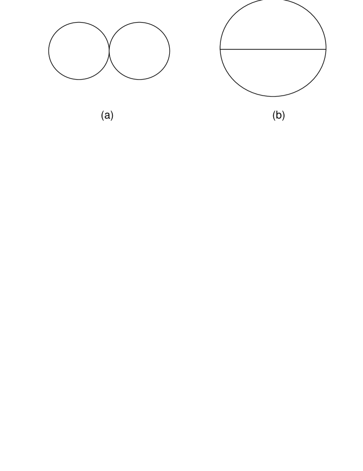
This situation is modified at the two loop order. We observe no gap and find that the phase transition is second order as shown in Fig.1 (c). Though Fig.1 (a) and Fig.1 (c) show the similar behaviour, it will be accident. The effective potential calculated up to the two loop order includes the contribution from the graphs, Fig.2 (a) and Fig.2 (b), with daisy resummation. On the other hand we can take into account the contribution from all the other graphs in addition to Fig.2 (a) and Fig.2 (b) within the approximation (16) by solving Eq.(19) automatically. The Fig.1 (a) accidentally coincides with Fig.1 (c).

\drawline[-50](220,113)(220,877) \path(220,113)(240,113) \path(1436,113)(1416,113) -0.0005\path(220,266)(240,266) \path(1436,266)(1416,266) -0.0004\path(220,419)(240,419) \path(1436,419)(1416,419) -0.0003\path(220,571)(240,571) \path(1436,571)(1416,571) -0.0002\path(220,724)(240,724) \path(1436,724)(1416,724) -0.0001\path(220,877)(240,877) \path(1436,877)(1416,877) 0\path(220,113)(220,133) \path(220,877)(220,857) 0\path(463,113)(463,133) \path(463,877)(463,857) 0.2\path(706,113)(706,133) \path(706,877)(706,857) 0.4\path(950,113)(950,133) \path(950,877)(950,857) 0.6\path(1193,113)(1193,133) \path(1193,877)(1193,857) 0.8\path(1436,113)(1436,133) \path(1436,877)(1436,857) 1\path(220,113)(1436,113)(1436,877)(220,877)(220,113) $\Im V(\phi)/\mu^{4}$ $\phi/\mu$ $T=5.0\mu$ $T=4.95\mu$\path(220,877)(220,877)(392,877)(564,877)(736,877)(908,877)(1080,877)(1252,877)(1424,877)(1436,877) \path(220,332)(220,332)(392,451)(564,707)(736,855)(908,876)(1080,877)(1252,877)(1424,877)(1436,877) \path(592,113)(736,575)(908,829)(1080,873)(1252,877)(1424,877)(1436,877)
Figure 3: Imaginary part of the effective potential near the critical temperature

For $T<T_{c}$ the effective potential develops a non-vanishing imaginary part at small $\bar{\phi}$ range. We show it in Fig.3. It should be noted that the sign of the imaginary part is always negative. It is consistent with the discussion in the previous subsection.

\path(220,113)(240,113) \path(1436,113)(1416,113) 0\path(220,222)(240,222) \path(1436,222)(1416,222) 10\path(220,331)(240,331) \path(1436,331)(1416,331) 20\path(220,440)(240,440) \path(1436,440)(1416,440) 30\path(220,550)(240,550) \path(1436,550)(1416,550) 40\path(220,659)(240,659) \path(1436,659)(1416,659) 50\path(220,768)(240,768) \path(1436,768)(1416,768) 60\path(220,877)(240,877) \path(1436,877)(1416,877) 70\path(220,113)(220,133) \path(220,877)(220,857) 0\path(463,113)(463,133) \path(463,877)(463,857) 0.2\path(706,113)(706,133) \path(706,877)(706,857) 0.4\path(950,113)(950,133) \path(950,877)(950,857) 0.6\path(1193,113)(1193,133) \path(1193,877)(1193,857) 0.8\path(1436,113)(1436,133) \path(1436,877)(1436,857) 1\path(220,113)(1436,113)(1436,877)(220,877)(220,113) $T_{c}/\mu$ $\lambda$ $\phi_{c}=0$ $\phi_{c}\neq 0$\path(1436,168)(1436,168)(828,190)(524,221)(372,266)(342,283)(281,353)(250,453)(235,593)(232,649)(226,871)(226,877)
Figure 4: Phase boundary

Evaluating the effective potential with varying the temperature, $T$, and the coupling constant, $\lambda$, we obtain the critical temperature as a function of $\lambda$ where the field expectation value disappears. We show the phase boundary on $T$-$\lambda$ plain in Fig.4.

The critical exponents are defined for the second-order phase transition. Around the critical temperature we expect that the susceptibility $\chi$, the expectation value $\phi_{c}$, and the specific heat $C$ behave as [40]

$$\chi\propto|t|^{-\gamma},\phi_{c}\propto|t|^{+\beta},C\propto|t|^{-\alpha},$$ (20)

where $t=(T-T_{c})/T$. Analysing the effective potential more precisely we can calculate the critical exponents $\gamma,\beta$, and $\alpha$. The susceptibility $\chi$ satisfies the following relation,

$$\xi\propto\rho^{-1},$$ (21)

where $\rho$ is the curvature of the effective potential at $\phi_{c}$.

Since the specific heat $C$ is given by the second derivative of the effective potential around the critical temperature, the effective potential $V(\phi_{c})$ behaves as

$$V(\phi_{c})\propto|t|^{2-\alpha}.$$ (22)
\path(220,113)(240,113) \path(836,113)(816,113) 0\path(220,252)(240,252) \path(836,252)(816,252) 0.2\path(220,391)(240,391) \path(836,391)(816,391) 0.4\path(220,530)(240,530) \path(836,530)(816,530) 0.6\path(220,669)(240,669) \path(836,669)(816,669) 0.8\path(220,808)(240,808) \path(836,808)(816,808) 1\path(288,113)(288,133) \path(288,877)(288,857) 4.8\path(425,113)(425,133) \path(425,877)(425,857) 4.9\path(562,113)(562,133) \path(562,877)(562,857) 5\path(699,113)(699,133) \path(699,877)(699,857) 5.1\path(836,113)(836,133) \path(836,877)(836,857) 5.2\path(220,113)(836,113)(836,877)(220,877)(220,113) $\phi_{c}/\mu$ $T/\mu$\path(836,113)(836,113)(822,113)(809,113)(795,113)(781,113)(768,113)(754,113)(740,113)(726,113)(713,113)(699,113)(685,113)(672,113)(658,113)(644,113)(631,241)(617,313)(603,365)(590,401)(576,433)(562,461)(549,486)(535,509)(521,530)(507,550)(494,568)(480,586)(466,602)(453,618)(439,633)(425,648)(412,662)(398,676)(384,689)(371,702)(357,714)(343,726)(330,737)(316,749)(302,760)(288,771)(275,781)(261,791)(247,802)(234,811)(220,821)(220,821)

(a) Field expectation value $\phi_{c}$

\path(220,113)(240,113) \path(836,113)(816,113) 0\path(220,254)(240,254) \path(836,254)(816,254) 0.05\path(220,396)(240,396) \path(836,396)(816,396) 0.1\path(220,537)(240,537) \path(836,537)(816,537) 0.15\path(220,679)(240,679) \path(836,679)(816,679) 0.2\path(220,820)(240,820) \path(836,820)(816,820) 0.25\path(288,113)(288,133) \path(288,877)(288,857) 4.8\path(425,113)(425,133) \path(425,877)(425,857) 4.9\path(562,113)(562,133) \path(562,877)(562,857) 5\path(699,113)(699,133) \path(699,877)(699,857) 5.1\path(836,113)(836,133) \path(836,877)(836,857) 5.2\path(220,113)(836,113)(836,877)(220,877)(220,113) $\rho/\mu$ $T/\mu$\path(836,225)(836,225)(822,216)(809,207)(795,199)(781,190)(768,182)(754,174)(740,166)(726,158)(713,150)(699,142)(685,135)(672,128)(658,121)(644,116)(631,119)(617,133)(603,155)(590,175)(576,194)(562,215)(549,239)(535,260)(521,282)(507,303)(494,326)(480,349)(466,371)(453,394)(439,416)(425,438)(412,460)(398,482)(384,505)(371,528)(357,550)(343,573)(330,595)(316,617)(302,639)(288,661)(275,684)(261,706)(247,728)(234,751)(220,773)(220,773)

(b) curvature $\rho$ at the minimum

\path(220,168)(240,168) \path(836,168)(816,168) -0.025\path(220,305)(240,305) \path(836,305)(816,305) -0.02\path(220,443)(240,443) \path(836,443)(816,443) -0.015\path(220,580)(240,580) \path(836,580)(816,580) -0.01\path(220,718)(240,718) \path(836,718)(816,718) -0.005\path(220,855)(240,855) \path(836,855)(816,855) 0\path(288,113)(288,133) \path(288,877)(288,857) 4.8\path(425,113)(425,133) \path(425,877)(425,857) 4.9\path(562,113)(562,133) \path(562,877)(562,857) 5\path(699,113)(699,133) \path(699,877)(699,857) 5.1\path(836,113)(836,133) \path(836,877)(836,857) 5.2\path(220,113)(836,113)(836,877)(220,877)(220,113) $V(\phi_{c})/\mu^{4}$ $T/\mu$\path(836,855)(836,855)(822,855)(809,855)(795,855)(781,855)(768,855)(754,855)(740,855)(726,855)(713,855)(699,855)(685,855)(672,855)(658,855)(644,855)(631,855)(617,854)(603,850)(590,846)(576,839)(562,831)(549,821)(535,810)(521,797)(507,783)(494,767)(480,750)(466,730)(453,710)(439,688)(425,665)(412,640)(398,614)(384,586)(371,557)(357,527)(343,495)(330,462)(316,428)(302,392)(288,355)(275,317)(261,277)(247,237)(234,194)(220,152)(220,152)

(c) Minimum of the effective potential $V(\phi_{c})$

Figure 5: Critical behaviour of $\phi_{c}$, $\rho$ and $V(\phi_{c})$

We examine the behaviour of $\rho,\phi_{c}$ ,and $V(\phi_{c})$ around the critical temperature and find the critical exponents $\gamma,\beta$ and $\alpha$. In Fig.5 the critical behaviour of $\rho,\phi_{c}$ and $V(\phi_{c})$ are shown as a function of the temperature. We numerically calculate the critical exponents from them. Our numerical results are presented in the table 1.222 Due to the instability in the explicit differencing method, we can not see the fine structure of the effective potential and can get only the rough values of the critical exponents. We need further numerical study to get more precise values.

Table 1: Critical exponents
our results Landau theory experimental results [41]
$\beta$ $\sim 0.5$ $0.5$ $0.33$
$\gamma$ $\sim 1$ $1$ $1.24$
$\alpha$ $\sim 0$ 00 $0.11$

The critical exponents within our approximation are independent of the coupling constant $\lambda$. We note that our results described in the present subsection remain unchanged even when we put the initial mass scale $M^{2}=T^{2}/4$ or $M^{2}=4T^{2}$.

4 Conclusion

We constructed the non-perturbative method to investigate the phase structure of $\lambda\phi^{4}$ theory. The derivative of the effective potential with respect to mass square was exactly expressed in terms of the full propagator at finite temperature. We found the partial differential equation for the effective potential with the replacement (16). We gave the initial condition by the 1 loop effective potential in the range where the perturbation theory is reliable. We numerically solved the partial differential equation and obtained the effective potential.

Though we made the approximation (16), we could find that the phase transition of $\lambda\phi^{4}$ theory is second order as it should be. Our method is very interesting because it can show the correct order of the phase transition. The approximation (16) may be fairy good.

We determined several critical exponents which roughly agree with those of Landau approximation. They are, however, rough values because it is very difficult to solve the nonlinear partial differential equation (17) numerically. We need elaborate a numerical study to obtain more accurate critical exponents.

The main problem of our non-perturbative method is how to improve the approximation to the full propagator. We cannot estimate the error from the approximation (16). We need improve the approximation to the full propagator in order to know the correction to the current result.

Our method is very promising since it can probe the region where the traditional perturbation theory breaks down.

Acknowledgements

The authors would like to thank Akira Niegawa and Jiro Arafune for useful discussions.

Appendix A The derivative of the effective potential in terms of the full propagator

The derivative of the effective potential $\displaystyle\frac{\partial V}{\partial m^{2}}$ can be represented by the full propagator. In this appendix we present details of the calculation of $\displaystyle\frac{\partial V}{\partial m^{2}}$ given in Eq.(4).

We consider the Lagrangian density which is defined by

$${\cal L}_{E}=-\frac{1}{2}\left(\frac{\partial\phi_{0}}{\partial\tau}\right)^{2}-\frac{1}{2}(\mbox{\boldmath$\nabla$}\phi_{0})^{2}-\frac{1}{2}m^{2}_{0}\phi^{2}_{0}-\frac{\lambda_{0}}{4!}\phi_{0}^{4}+J_{0}\phi_{0},$$ (23)

where the suffix 00 denotes the bare quantities.

We adopt the mass-independent renormalization procedure and represent the effective potential as a function of renormalized quantities. The renormalization constants $Z$ and renormalized quantities are introduced through transformations

$$\begin{array}[]{rcl}\phi_{0}&=&Z_{\phi}^{1/2}\phi,\\ m_{0}&=&Z_{m}^{1/2}m,\\ \lambda_{0}&=&Z_{\lambda}\lambda,\\ J_{0}&=&Z_{\phi}^{-1/2}J.\end{array}$$ (24)

Using these renormalization constants and renormalized quantities, we separate the Lagrangian density (23) into the tree part ${\cal L}_{1}$ and the counter term part ${\cal L}_{ct}$ as [40, 42]

$${\cal L}_{E}={\cal L}_{1}[\phi]+{\cal L}_{ct}[\phi]+(J_{1}+J_{ct})\phi,$$ (25)

where $J_{1}+J_{ct}\equiv J$. The laglangian density ${\cal L}_{1}$ and ${\cal L}_{ct}$ are given by

$$\left\{\begin{array}[]{rcl}{\cal L}_{1}[\phi]&\equiv&\displaystyle-\frac{1}{2}\left(\frac{\partial\phi}{\partial\tau}\right)^{2}-\frac{1}{2}(\mbox{\boldmath$\nabla$}\phi)^{2}-\frac{1}{2}m^{2}\phi^{2}-\frac{\lambda}{4!}\phi^{4},\\ {\cal L}_{ct}[\phi]&\equiv&\displaystyle-\frac{1}{2}(Z_{\phi}-1)\left[\left(\frac{\partial\phi}{\partial\tau}\right)^{2}+(\mbox{\boldmath$\nabla$}\phi)^{2}\right]-\frac{1}{2}(Z_{m}Z_{\phi}-1)m^{2}\phi^{2}\\ &&\displaystyle-\frac{\lambda}{4!}(Z_{\lambda}Z_{\phi}^{2}-1)\phi^{4}.\end{array}\right.$$ (26)

Here we separate the external source $J$ into $J_{1}$ and $J_{ct}$, which satisfy the following equations:

$$\left\{\begin{array}[]{rcl}\displaystyle\left.\frac{\partial{\cal L}_{1}}{\partial\phi}\right|_{\phi=\bar{\phi}}+J_{1}&=&0,\\ \langle\phi\rangle_{J}&=&\bar{\phi}.\end{array}\right.$$ (27)

We expand the field $\phi(x)$ around the classical background $\bar{\phi}$,

$$\phi(x)=\bar{\phi}+\eta(x),$$ (28)

and then $\eta(x)$ satisfies

$$\langle\eta\rangle_{J}=0.$$ (29)

In terms of $\bar{\phi}$ and $\eta(x)$ Eq.(26) is rewritten as

$\displaystyle{\cal L}_{1}+J_{1}\phi$ $\displaystyle=$ $\displaystyle-\frac{1}{2}m^{2}\bar{\phi}^{2}-\frac{\lambda}{4!}\bar{\phi}^{4}+J_{1}\bar{\phi}-\frac{1}{2}\left[\left(\frac{\partial\eta}{\partial\tau}\right)^{2}+(\mbox{\boldmath$\nabla$}\eta)^{2}\right]$ (30)
$\displaystyle-\frac{1}{2}\left(m^{2}+\frac{\lambda}{2}\bar{\phi}^{2}\right)\eta^{2}-\frac{\lambda}{3!}\bar{\phi}\eta^{3}-\frac{\lambda}{4!}\eta^{4}$
$\displaystyle\equiv$ $\displaystyle{\cal L}_{1}(\bar{\phi})+{\cal L}^{\prime}_{1}[\eta],$

and

$\displaystyle{\cal L}_{ct}+J_{ct}\phi$ $\displaystyle=$ $\displaystyle-\frac{1}{2}(Z_{m}Z_{\phi}-1)m^{2}\bar{\phi}^{2}-\frac{\lambda}{4!}(Z_{\lambda}Z_{\phi}^{2}-1)\bar{\phi}^{4}+J_{ct}\bar{\phi}$ (31)
$\displaystyle\left[-(Z_{m}Z_{\phi}-1)m^{2}\bar{\phi}-\frac{\lambda}{3!}(Z_{\lambda}Z_{\phi}^{2}-1)\bar{\phi}^{3}+J_{ct}\right]\eta$
$\displaystyle-\frac{1}{2}(Z_{\phi}-1)\left[\left(\frac{\partial\eta}{\partial\tau}\right)^{2}+(\mbox{\boldmath$\nabla$}\eta)^{2}\right]-\frac{1}{2}(Z_{\phi}Z_{m}-1)m^{2}\eta^{2}$
$\displaystyle-\frac{\lambda}{2}(Z_{\lambda}Z_{\phi}^{2}-1)\bar{\phi}^{2}\eta^{2}-\frac{\lambda}{3!}(Z_{\lambda}Z_{\phi}^{2}-1)\bar{\phi}\eta^{3}-\frac{\lambda}{4!}(Z_{\lambda}Z_{\phi}^{2}-1)\eta^{4}$
$\displaystyle\equiv$ $\displaystyle{\cal L}_{ct}(\bar{\phi})+K\eta+{\cal L}^{\prime}_{ct}[\eta],$

where $K$ is defined by

$$K\equiv-(Z_{m}Z_{\phi}-1)m^{2}\bar{\phi}-\frac{\lambda}{3!}(Z_{\lambda}Z_{\phi}^{2}-1)\bar{\phi}^{3}+J_{ct}.$$ (32)

From Eq.(29), $\eta(x)$ satisfies

$$\langle\eta\rangle_{K}=0.$$ (33)

The generating functional $W_{T}[J]$ for connected Green functions is given by

$$Z_{T}[J]=e^{W_{T}[J]}.$$ (34)

The effective action $\Gamma_{T}(\bar{\phi})$ is defined as the Legendre transformation of $W_{T}[J]$. In the spacetime with the translational invariance the effective potential $V(\bar{\phi})$ is proportional to the effective action. The effective potential $V(\bar{\phi})$ is

$$-\frac{\Omega}{T}V({\bar{\phi}})=\Gamma_{T}(\bar{\phi})=W_{T}[J]-\frac{\Omega}{T}\bar{\phi}J,$$ (35)

where $\displaystyle\Omega=\int d^{3}\mbox{\boldmath$x$}$ and the new variable $\bar{\phi}$ is given by

$$\frac{\delta}{\delta J(y)}W_{T}[J]=\bar{\phi}(y)=\bar{\phi}=\mbox{const}.$$ (36)

Substituting Eqs.(30) and (31) into Eq.(25), we rewrite the generating functional $Z_{T}$ as a functional of renormalized quantities,

$\displaystyle Z_{T}$ $\displaystyle=$ $\displaystyle\exp\left\{\frac{\Omega}{T}\left[{\cal L}_{1}(\bar{\phi})+{\cal L}_{ct}(\bar{\phi})+(J_{1}+J_{ct})\bar{\phi}\right]\right\}$ (37)
$\displaystyle\times\int D[\eta]\exp\int^{1/T}_{0}d\tau\int d^{3}\mbox{\boldmath$x$}\left({\cal L}^{\prime}_{1}[\eta]+{\cal L}^{\prime}_{ct}[\eta]+K\eta\right)$
$\displaystyle\equiv$ $\displaystyle\exp\left\{\frac{\Omega}{T}\left[{\cal L}_{1}(\bar{\phi})+{\cal L}_{ct}(\bar{\phi})+(J_{1}+J_{ct})\bar{\phi}\right]\right\}Z^{\prime}(K).$

Taking into account Eqs.(34) and (35), we obtain the effective potential from Eq.(37):

$$V(\bar{\phi})=-\left[{\cal L}_{1}(\bar{\phi})+{\cal L}_{ct}(\bar{\phi})\right]-\frac{T}{\Omega}\log Z^{\prime}(K).$$ (38)

In the mass-independent renormalization procedure the renormalization constants $Z$ are independent of the mass $m$. We easily differentiate the effective potential $V$ by the mass square $m^{2}$ and get

$\displaystyle\frac{\partial V(\bar{\phi})}{\partial m^{2}}$ $\displaystyle=$ $\displaystyle\left[\frac{1}{2}\bar{\phi}^{2}+\frac{1}{2}(Z_{m}Z_{\phi}-1)\bar{\phi}^{2}\right]$
$\displaystyle-\frac{T}{\Omega}\frac{1}{Z^{\prime}}\int D[\eta]\left[-\frac{1}{2}\eta^{2}+\frac{\partial K}{\partial m^{2}}\eta-\frac{1}{2}(Z_{m}Z_{\phi}-1)\eta^{2}\right]$
$\displaystyle\times\exp\int^{1/T}_{0}d\tau\int d^{3}\mbox{\boldmath$x$}\left({\cal L}^{\prime}_{1}[\eta]+{\cal L}^{\prime}_{ct}[\eta]+K\eta\right)$
$\displaystyle=$ $\displaystyle\left[\frac{1}{2}\bar{\phi}^{2}+\frac{1}{2}(Z_{m}Z_{\phi}-1)\bar{\phi}^{2}+\frac{1}{2}\langle\eta^{2}(0)\rangle+\frac{1}{2}(Z_{m}Z_{\phi}-1)\langle\eta^{2}(0)\rangle\right],$

where we use Eq.(33) [34].

For $\lambda\phi^{4}$ theory the two-point function $\langle\eta^{2}(0)\rangle$ in Eq.(A) is rewritten as

$\displaystyle\langle\eta^{2}(0)\rangle$ $\displaystyle=$ $\displaystyle\int^{1/T}_{0}d\tau\int d^{3}\mbox{\boldmath$x$}\delta^{3}(\mbox{\boldmath$x$})\delta_{T}(\tau)\langle\eta(\mbox{\boldmath$x$},\tau)\eta(\mbox{\boldmath$0$},0)\rangle$
$\displaystyle=$ $\displaystyle T\sum^{\infty}_{n=-\infty}\int\frac{d^{3}\mbox{\boldmath$p$}}{(2\pi)^{3}}\int^{1/T}_{0}d\tau\int d^{3}\mbox{\boldmath$x$}e^{i(\mbox{\boldmath$xp$}+\omega_{n}\tau)}\langle\eta(\mbox{\boldmath$x$},\tau)\eta(\mbox{\boldmath$0$},0)\rangle$
$\displaystyle=$ $\displaystyle T\sum^{\infty}_{n=-\infty}\int\frac{d^{3}\mbox{\boldmath$p$}}{(2\pi)^{3}}\frac{1}{\omega_{n}^{2}+\mbox{\boldmath$p$}^{2}+m^{2}+\frac{\lambda}{2}\bar{\phi}^{2}+\Pi},$

where $\omega_{n}=2\pi nT$ due to the periodic boundary condition for Bose fields and $\Pi=\Pi(\mbox{\boldmath$p$}^{2},-p_{0}^{2},\bar{\phi},m^{2},T)$ is the full self-energy. Substituting Eq.(A) into Eq.(A), we express the derivative of the effective potential in terms of the full propagator,

$\displaystyle\frac{\partial V}{\partial m^{2}}=\frac{1}{2}\bar{\phi}^{2}+\frac{T}{2}\sum^{\infty}_{n=-\infty}\int\frac{d^{3}\mbox{\boldmath$p$}}{(2\pi)^{3}}\frac{1}{\omega_{n}^{2}+\mbox{\boldmath$p$}^{2}+m^{2}+\frac{\lambda}{2}\bar{\phi}^{2}+\Pi}$ (41)
$\displaystyle+(Z_{m}Z_{\phi}-1)\left[\frac{1}{2}\bar{\phi}^{2}+\frac{T}{2}\sum^{\infty}_{n=-\infty}\int\frac{d^{3}\mbox{\boldmath$p$}}{(2\pi)^{3}}\frac{1}{\omega_{n}^{2}+\mbox{\boldmath$p$}^{2}+m^{2}+\frac{\lambda}{2}\bar{\phi}^{2}+\Pi}\right].$

Using the residue theorem, we convert the frequency sum $\displaystyle T\sum^{\infty}_{n=-\infty}$ to contour integrals. As long as $\Pi$ has no singularity along the imaginary $p_{0}$ axis, Eq.(41) naturally separates into a piece which contains a Bose factor and a piece which does not [12, 37],

$\displaystyle\frac{\partial V}{\partial m^{2}}$ $\displaystyle=$ $\displaystyle\frac{1}{2}\bar{\phi}^{2}+\frac{1}{2\pi i}\int^{+i\infty+\epsilon}_{-i\infty+\epsilon}dp_{0}\int\frac{d^{3}\mbox{\boldmath$p$}}{(2\pi)^{3}}\frac{1}{-p_{0}^{2}+\mbox{\boldmath$p$}^{2}+m^{2}+\frac{\lambda}{2}\bar{\phi}^{2}+\Pi}\frac{1}{e^{p_{0}/T}-1}$ (42)
$\displaystyle+\frac{1}{4\pi i}\int^{+i\infty}_{-i\infty}dp_{0}\int\frac{d^{3}\mbox{\boldmath$p$}}{(2\pi)^{3}}\frac{1}{-p_{0}^{2}+\mbox{\boldmath$p$}^{2}+m^{2}+\frac{\lambda}{2}\bar{\phi}^{2}+\Pi}$
$\displaystyle+(Z_{m}Z_{\phi}-1)\biggl{[}\frac{1}{2}\bar{\phi}^{2}$
$\displaystyle+\frac{1}{2\pi i}\int^{+i\infty+\epsilon}_{-i\infty+\epsilon}dp_{0}\int\frac{d^{3}\mbox{\boldmath$p$}}{(2\pi)^{3}}\frac{1}{-p_{0}^{2}+\mbox{\boldmath$p$}^{2}+m^{2}+\frac{\lambda}{2}\bar{\phi}^{2}+\Pi}\frac{1}{e^{p_{0}/T}-1}$
$\displaystyle+\frac{1}{4\pi i}\int^{+i\infty}_{-i\infty}dp_{0}\int\frac{d^{3}\mbox{\boldmath$p$}}{(2\pi)^{3}}\frac{1}{-p_{0}^{2}+\mbox{\boldmath$p$}^{2}+m^{2}+\frac{\lambda}{2}\bar{\phi}^{2}+\Pi}\biggr{]}.$

References

  • [1] D. A. Kirzhnits and A. D. Linde, Phys. Lett. B42 (1972) 471.
  • [2] M. E. Shaposhnikov, hep-ph/9610247.
  • [3] P. Arnold, Proceedings of Quarks ’94 (1994) 71 (hep-ph/9410294).
  • [4] M. E. Carrington, Phys. Rev. D45 (1992) 2933.
  • [5] P. Arnold and O. Espinosa, Phys. Rev. D47 (1993) 3546.
  • [6] L. Dolan and R. Jackiw, Phys. Rev. D9 (1974), 3320.
  • [7] S. Weinberg, Phys. Rev. D9 (1974) 3357.
  • [8] K. Takahashi, Z. Phys. C26 (1985) 601.
  • [9] P. Fendley, Phys. Lett. B196 (1987) 175.
  • [10] W. Buchmuller, Z. Fodor and A. Hebecker, Phys. Lett. B331 (1994) 131.
  • [11] Z. Fodor and A. Hebecker, Nucl.Phys. B432 (1994) 127.
  • [12] J. I. Kapsta, Finite Temperature Field Theory (Cambridge Univ. Press, 1989).
  • [13] M. Le. Bellac, Thermal Field Theory (Cambridge Univ. Press, 1996).
  • [14] Z. Fodor, J. Hein, K. Jansen, A. Jaster and I. Montvay,
    Nucl. Phys. B439 (1995) 147.
  • [15] F. Csikor, Z. Fodor, J. Hein, K. Jansen, A. Jaster and I. Montvay,
    Nucl.Phys. Proc. Suppl. 42 (1995) 569.
  • [16] M. Gürtler, E.-M. Ilgenfritz and A. Schiller, Phys. Rev. D56 (1997) 3888.
  • [17] M. Guertler, E.-M. Ilgenfritz , J. Kripfganz, H. Perltand and A. Schiller,
    Nucl. Phys. B483 (1997) 383.
  • [18] K. Kajantie, M. Laine, K. Rummukainen and M. E. Shaposhnikov,
    Phys. Rev. Lett. 77 (1996) 2887; hep-lat/9612006; hep-ph/9704416.
  • [19] Y. Aoki, Phys. Rev. D56 (1997) 3860.
  • [20] J. Cornwall, R. Jackiw, and E. Tomboulis, Phys. Rev. D10 (1974) 2428.
  • [21] G. Amelino-Camelia and S.-Y. Pi, Phys. Rev. D47 (1993) 2356;
    G. Amelino-Camelia, Phys. Rev. D49 (1994) 2740.
  • [22] P. Arnold and L. G. Yaffe, Phys. Rev. D49 (1994) 3003.
  • [23] P. Ginsparg, Nucl. Phys. B170 (1980) 388.
  • [24] T. Appelquist and R. Pisarski, Phys. Rev. D23 (1981) 2305.
  • [25] S. Nadkarni, Phys. Rev. D27 (1983) 917; Phys. Rev. D38 (1988) 3287.
  • [26] N.P. Landsman, Nucl. Phys. B322 (1989) 498.
  • [27] K. Farakos, K. Kajantie, K. Rummukainen and M. Shaposhnikov,
    Nucl. Phys. B442 (1995) 317.
  • [28] W. Buchmuller and O. Philipsen, Nucl. Phys. B443 (1995) 47.
  • [29] T. R. Morris and M.D. Turner, hep-th/9704202.
  • [30] M. D’Attanasio and T.R. Morris, Phys. Lett. B378 (1996) 213.
  • [31] K. Aoki, K. Morikawa, W. Souma, J. Sumi and H. Terao,
    Prog. Theor. Phys. 95 (1996) 409.
  • [32] J. Adams, J. Berges, S. Bornholdt, F. Freire, N. Tetradis and C. Wetterich,
    Mod. Phys. Lett. A10 (1995) 2367.
  • [33] B. Bergerhoff and C. Wetterich Nucl. Phys. B440 (1995) 171.
  • [34] I. T. Drummond, R. R. Horgan, P. V. Landshoff and A. Rebhan,
    Phys. Lett. B398 (1997) 326.
  • [35] A. D. Linde, Phys. Lett. B96 (1980) 289;
    D. Gross, R. Pisarski and L. Yaffe, Rev. Mod. Phys. 53 (1981) 43.
  • [36] T. Mastubara, Prog. Theor. Phys. 14 (1955) 351.
  • [37] P. D. Morley and M. B. Kislinger, Phys. Rep. 51 (1979)63.;
  • [38] E. Weinberg and A. Wu, Phys. Rev. D36 (1987) 2474.
  • [39] W. H. Press, B. P. Flannery, S. A. Teukolsky and W. T. Vetterling,
    Numerical Recipes in C (Cambridge Univ. Press, 1988).
  • [40] M. E. Peskin and D. V. Schroeder, An Introduction to the Quantum Field Theory, (Addison-Wesley Pub. Co., 1995).
  • [41] J. Zinn-Justin, Quantum Field Theory and Critical Phenomena, (Oxford Univ. Press, 1996).
  • [42] R. Jackiw, Phys. Rev. D9 (1974) 1686.