On the Geometry behind $N=2$ Supersymmetric Effective Actions in Four Dimensions.

Abstract

An introduction to Seiberg-Witten theory and its relation to theories which include gravity.

1 Introduction

In the last years it has become clear that consistency requirements restrict the non-perturbative properties of supersymmetric theories much more then previously thought. In fact it turned out that such theories cannot be consistently “defined” without referring to their non-perturbative structure.

The prototypical examples are the $N=2$ $SU(2)$ supersymmetric Yang-Mills theories of Seiberg and Witten [1]. Self-consistency seems to require a duality to be at work, which interchanges an electrical and a magnetic description of the same low energy theory. A short introduction into this duality will follow in section (2). The set of states, which are elementary in one description, are solitonic in the other. Depending on the scale one of the descriptions is preferred because its coupling is weak. In particular the description of the effective $SU(2)$ gauge theory can be replaced in its strongly coupled infrared regime by a magnetic $U(1)$ gauge theory, which couples weakly to massless magnetic monopoles. Vice versa, if one starts at low scales with the weakly coupled magnetic $U(1)$ theory one gratefully notices that it can be replaced by the asymptotically free $SU(2)$ theory before it hits its Landau pole in the ultraviolet. These theories are probably the first examples of globally consistent nontrivial continuum quantum field theories in four dimensions. A review of these theories is given in section (3).

What is known about these theories, namely the exact masses of the BPS states and the exact gauge coupling, is so far not derived from a first principle high energy formulation but rather from some knowledge of the symmetries of the microscopic theory and global consistency conditions of the low energy Wilsonian action, as defined in section (3.1). The reconstruction from consistency requirements is subject of section (3.2), it leads in particular to an uniformization problem, whose solution is discussed in subsection (3.2.1). It seems rather difficult to go beyond these results without a deeper understanding the microscopic theory.

The BPS states are the lightest states, which carry electric or magnetic charge. Their mass is proportional to a topological central term in the supersymmetry algebra, see Appendix A. The BPS masses and the gauge coupling have a remarkable geometrical interpretation, as described in section (4). In particular for $SU(2)$ theories there is an auxiliary elliptic curve, in real coordinates a surface, whose volume gives the gauge coupling and whose period integrals give the masses. For higher rank groups special Riemann surfaces can be constructed, which encode these informations in a similar way. The discussion of these auxiliary surfaces is subject of section (4.2).

To include gravity one has essentially to replace the Riemann surfaces by a suitable Calabi-Yau threefold and to consider the effective action of the ten dimensional type II “string” theory compactification on the Calabi-Yau manifold. Basic properties of Calabi-manifolds are summarized in section (5). As in the pure gauge theory case one can allow for considerable ignorance of the details of the microscopic theory, which describes gravity, and can nevertheless obtain certain properties of the effective theory exactly. Since the periods are proportional to the masses and vanish at the degeneration points of the manifold, the question about possible light spectra in the effective action becomes a question about the possible degeneration, or in other words, an issue of singularity theory. What happens at the possible degeneration sheds, on the other hand, light on the microscopic theory. This story is familiar from the type II/heterotic string duality [3] in six dimensions. The singularities a $K3$ can acquire are the classified $ADE$ surface singularities, see sect. 8, and lead for the type IIa theory by wrapping of two-branes to precisely the massless non-abelian gauge bosons which are required to match the gauge symmetry enhancements of the heterotic string on $T4$ [4] [5]. The possible singularities of Calabi-Yau threefolds are far richer and lead not only to gauge theories with or without matter but also to exotic limits of $N=2$ theories in four dimensions which fit a microscopic description in terms of non critical string theories.

The perturbative string sector of the type II theory is less complete then the magnetic or the electric field theory formulation of Seiberg-Witten, it contains neither electrically nor magnetically charged states. The welcome flip side of this coin is that the magnetically and electrically charged states, which are solitonic, appear more symmetrically. Both types can be understood as wrappings of the $D$-branes of the Type II theory around supersymmetric cycles of the Calabi-Yau manifold, see section (6.1.3). In the type IIb theory solitonic states arise by wrapping three branes around sypersymmetric Calabi-Yau three-cycles. They can lead to solitonic hypermultiplets, which were interpreted as extremal black holes in [6], or to solitonic vector multiplets [9]. In the appropriate double scaling limit, which decouples gravity, $M_{pl}\rightarrow\infty$, and the string effects, $\alpha^{\prime}\rightarrow 0$, [8] these solitons are identified with the Seiberg-Witten monopole and non-abelian gauge bosons respectively [9].

Mirror symmetry maps type IIb theory to type IIa theory, the odd branes to even branes and the odd supersymmetric cycles to even supersymmetric cycles. In the type IIa theory the non-abelian gauge bosons can now be understood as two-branes wrapped around non-isolated supersymmetric two-cycles, which are in the geometrical phase of the CY manifold nothing else then non-isolated holomorphic curves. One can easily “geometrical engineer” configurations of such holomorphic curves, which will lead in the analogous scaling limit [8] to prescribed gauge groups, also with controllable matter content [10]. Using local mirror symmetry [10] it is possible to rederive in this way the Seiberg-Witten effective theory description by the Riemann surfaces from our present understanding of the non-perturbative sector of the type IIa string alone.

One very important aspect of the embedding of the $N=2$ field theory into the type II theory on CY manifolds is that the field theory coupling constant is realized in the type II description as a particular geometrical modulus. The strong-weak coupling duality is accordingly realized as a symmetry which acts geometrically on the CY moduli. In fact all properties of the non-perturbative field theory can be related to geometrical properties of the CY manifold, e.g. the space-time instanton contributions of Seiberg-Witten are related to invariants of rational curves embedded in the Calabi-Yau manifold, etc. [10].

In the type IIb theory the solitonic states originate most symmetrically, namely from the wrapping of three-branes. We do not have really a non-perturbative formulation of the type II theory yet. One can try to keep the advantages of the symmetric appearance of the solitons and yet simplify the situation by modifying the above limit to just decouple gravity [9]. As reviewed in [36] this gives rise to non-critical string theories in six dimensions and a quite intuitive picture for the solitonic states as $D$-strings wound around the cycles of the Riemann surfaces. At this moment we do not understand these non-critical string theories well enough to infer properties which go much beyond what can be learned from the geometry of the singularities, rather at the moment the geometrical picture wins and predicts some basic features of these yet illusive theories.

An important conceptual and technical tool in the analysis is mirror symmetry. Aspects of this will be discussed it section (6.1). This includes a discussion of some properties of the relevant branes sec. (6.1.3), special Kähler geometry sec. (6.2.1), the deformation of the complexified Kähler structure sec. (6.2.2) with special emphasis on the point of large Kähler structure sec. (6.2.3) as well as the main technical tool, the deformation theory of the complex structure sec. (6.2.4). The duality between the heterotic string and the type II string is shortly discussed in sec. (6.3).

We find it very useful to present in some detail an example where all the concepts presented in these lectures come together, the so called $(ST)$-model, which corresponds to a simple $K3$ fibration Calabi-Yau, sec. (7). In principle it should be possible to try to understand this example first and go backwards in the text when more background material is needed.

2 Electric-magnetic duality and BPS-states

Before we turn to the $N=2$ case we shall give a short review of the concept of $S$-duality in field theory and in particular in $N=4$ supersymmetric theories. This is in order to introduce some concepts, where they are realized in the simplest way, and to prepare for the more complicated situation in $N=2$ theories. There exist already highly recommendable reviews [11], [13] on the subject, so we will be very brief here.

The semi-classical mass bound saturated for the Prasad-Sommerfield-Bogomol’nyi (BPS) states in a pure $SU(2)$ gauge theory without matter and a Higgs in the adjoint with potential $V={\lambda\over 4}(\phi^{a}\phi^{a}-v)^{2}$ is given by

$$M\geq|v(n_{e}+\tau n_{m})|.$$ (2.1)

Here $n_{e}$ and $n_{m}$ are integral electric and magnetic charge quantum numbers of the state and $\tau$ is a combination of the gauge coupling and the $\theta$-angle

$$\tau={\theta\over 2\pi}+{4\pi i\over g^{2}}\ .$$ (2.2)

The mass of the elementary purely electrically charged $W^{\pm}$ bosons is of course just given by the Higgseffect, as reproduced by (2.1). The purely magnetic states are solitonic, the simplest being the t’Hooft-Polyakov monopole configuration. The semiclassical mass bound for these configurations has been derived in [15] (see [12] for a review).

There is a very remarkable fractional linear symmetry (see below, why only integer shifts $\tau\rightarrow\tau+a$, $a\in\hbox{ZZ}$ are considered) in these formulas

$$\begin{array}[]{rl}{\bf S}:&\left\{\begin{array}[]{rl}n_{e}&\rightarrow n_{m}\cr n_{m}&\rightarrow-n_{e}\cr\tau&\rightarrow-{1\over\tau}\cr v&\rightarrow v\tau\end{array}\right.\\[11.38109pt] {\bf T}:&\left\{\begin{array}[]{rl}n_{e}&\rightarrow n_{e}-n_{m}\cr n_{m}&\rightarrow n_{m}\cr\tau&\rightarrow\tau+1\cr v&\rightarrow v\end{array}\right.\end{array}$$ (2.3)

which generate a $PSL(2,\hbox{ZZ})$ action

$$\tau\mapsto{A\tau+B\over C\tau+D}$$ (2.4)

on $\tau$ with $A,B,C,D\in\hbox{ZZ}$ and $AD-BC=1$ as well as an $SL(2,\hbox{ZZ})$ action on the electro-magnetic ‘charge’ vector

$$\left(\matrix{n_{m}\cr n_{e}}\right)\mapsto\left(\matrix{D&-C\cr-B&A}\right)\left(\matrix{n_{m}\cr n_{e}}\right)$$

The S-action, which exchanges in particular the $W^{\pm}$ bosons with t’Hooft-Polyakov monopoles and inverts the gauge coupling (for $\theta=0$), was conjectured by Montonen and Olive [16] to be in some sense a symmetry in the full quantum theory. It is obvious that a naive microscopic realization cannot possibly work in a normal quantum field theory:

$\bullet$ Because the gauge bosons and the monopoles are not in the same Lorentz group representation

$\bullet$ In the quantum theory the coupling ${4\pi i\over g^{2}(\mu)}$ will have different scale dependence in the original theory and its dual, which make a simple interpretation of the inversion symmetry impossible.

$\bullet$ The semiclassical analysis of the mass relied on the assumption that $V=0$ for the BPS configuration [15], which will be invalidated by quantum corrections.

All these objections evaporate however in a theory with $N=4$ global supersymmetry, the maximal possible in four dimensions. Only here the gauge bosons and the monopoles are both in the same susy multiplet; the ultrashort $N=4$ multiplet. The coupling does not run in $N=4$ theories as the beta function is exactly zero, in fact the full theory is believed not only to be scale invariant but actually conformal. Finally the potential in the supersymmetric quantum theory is $V\equiv 0$.

As for the validity of (2.1) in the quantum theory, it was shown in [17] that the supersymmetry algebra gets central extensions in the presence of non-trivial vacuum configurations. A simple analysis of the representation theory of supersymmetry algebras with $N$ (even) supersymmetry generators in the presence of central extensions $Z_{i}$, see app. A and Ch. II of [88], shows that the mass of all multiplets is bounded by $M\geq|Z_{i}|$, $i=1,\ldots,(N/2)$ and the multiplets whose mass is actually $M=|Z_{i}|$, $\forall\,i$, consist of $2^{N}$ degrees of freedom, while the generic ones, with the minimal spin difference in the multiplet ($N/2$), have $2^{2N}$ degrees of freedom. The central charge as calculated in [17] from the anti-commutator of the super-charges in non-trivial vacuum configurations reproduces the semiclassical formula (2.1), i.e. $Z=v(n_{e}+\tau n_{m})$. If the existence of BPS saturated states is established by a calculation in the semiclassical regime the supersymmetry algebra protects these states from wandering off the bound, neither by perturbative quantum effects nor by non-perturbative effects, as long as the supersymmetry is unbroken.

Because the $\theta$-angle appears in front of the topological term in the Lagrangian

$$\begin{array}[]{rl}{\cal L}&=-{1\over 4g^{2}}F^{\mu\nu}F_{\mu\nu}-{\theta\over 32\pi^{2}}F^{\mu\nu}{{}^{*}}F_{\mu\nu}\\[5.69054pt] &=-{1\over 32\pi}{\rm Im}\biggl{(}\tau(F^{\mu\nu}+i{{}^{*}}F^{\mu\nu})(F_{\mu\nu}+i{{}^{*}}F_{\mu\nu})\biggr{)}\end{array}$$ (2.5)

only $\theta$-shifts by an integer $\tau\rightarrow\tau+1$ alter the classical action by a multiple of $2\pi$ and hence the weight factor in the path integral by an irrelevant phase shift. In this context it is important to note that an $n$-instanton effect in this normalization will be weighted by $e^{2\pi in\tau}$. This is the reason for the integrality condition which leads to $SL(2,\hbox{ZZ})$ as duality group. At quantum level it is again only the $N=4$ theory which allows for the definition of a microscopic $\theta$-angle.

The electric and magnetic charges as defined from the Noether current of a dyon with quantum numbers $(n_{m},n_{e})$ are $q=en_{e}-{\theta e\over 2\pi}n_{m}$ and $p={4\pi\over e}n_{m}$. For consistent quantization, pairs of dyons $(p,q)$ $(p^{\prime},q^{\prime})$ must satisfy the Dirac-Zwanziger quantization condition

$$\begin{array}[]{rl}qp^{\prime}-q^{\prime}p&=4\pi(n_{e}n^{\prime}_{m}-n^{\prime}_{e}n_{m})\cr&=2\pi n,\ \ n\in\hbox{ZZ}\cr\end{array}$$ (2.6)

actually here with $n/2\in\hbox{ZZ}$, which is good as we want later to include quarks which have half-integer charges in this units. The condition (2.6) generalizes immediately to theories with $r$ electric charges and $r$ magnetic charges, where it requires integrality of the sympletic form $\vec{n}_{e}\vec{n}^{\prime}_{m}-\vec{n}^{\prime}_{e}\vec{n}_{m}=n$. Quite generally one can argue [22] that a theory containing simultaneously massless states for which (2.6) does not vanish is conformal (and does not admit a local Lagrangian description).

Figure 1: Charges of dyons, which fulfill the Dirac-Zwanziger quantization condition, lie on a lattice $\Lambda$ spanned by $e\tau$ and $e$ in the complex plane ($e$ is set to one).

Under the mild assumption that $W^{\pm}$-bosons exist in an $N=4$ theory as stable BPS states and $\tau$ is a generic complex number, i.e. the lattice $\Lambda$ in figure 1 is not degenerate, $S$-duality makes very non-trivial predictions: The existence of the dyonic BPS states in the $SL(2,\hbox{ZZ})$ orbit. These must be stable if their decay into other BPS states is forbidden by mass and charge conservation. By (2.1) and the assumption that $\tau$ is generic, stability means simply that $(n_{e},n_{m})$ must be co-prime integers. Some of these predicted stable multimonopole configurations have been found in [19] for the (broken) $SU(2)$, which has triggered renewed interest into $S$-duality. For $SU(3)$ analogous predictions were checked in [20]. The relevant discrete duality group for the latter case is $SP(4,\hbox{ZZ})$.

A more genuine strong coupling test was performed in twisted $N=4$ theories on various manifolds [21].

3 $N=2$ supersymmetric Yang-Mills theory

From the last section it is clear that the $S$-duality cannot be realized as a symmetry in the microscopic $N=2$ $SU(2)$ Yang-Mills gauge theory. As it turned out from the analysis of Seiberg and Witten, a subgroup of $SL(2,\hbox{ZZ})$ (or $SP(2\times{\rm rank}(G),\hbox{ZZ})$ for general gauge group $G$) is realized in this case on the abelian gauge fields of the effective action.

This symmetry and an intriguing combination of microscopic and macroscopic arguments makes it possible to determine the terms up to two derivatives in the effective actions exactly. In fact $N=2$ supersymmetry implies that the functions, which determine the $N=2$ effective action to this order, are holomorphic and, as one might expect, they are closely related to automorphic forms of the relevant symmetry groups, which are in the simplest cases subgroups of $SL(2,\hbox{ZZ})$. Reviews on the subject can be found in [35] [36] [37].

The theory of automorphic functions of subgroups of $SL(2,\hbox{ZZ})$ is an old and extremely well studied mathematical subject, so that once the group is known the functions can be quickly related (in many different ways) to well known ones. This theory has been also used in [44] [45] to clarify some assumption made in [1] [2]. We will review some aspects of this approach. However the theory of automorphic function becomes more difficult and less studied for the multi parameter cases involving subgroups of $SP(2\times{\rm rank}(G),\hbox{ZZ})$.

Therefore we focus in section (4) mainly on a closely related approach, which identifies the electro-magnetic charge lattice $\Lambda$ with the integral homology lattice $H^{1}(X,\hbox{ZZ})$ of an auxiliary Riemann surface $X$. In this approach the bilinear form (2.6) will be identified with the intersection form on $X$ and the relevant functions, which determine the effective action, can be obtained from period integrals of the Riemann surface.

If one includes gravity, which has to be done by embedding the supergravity in string theory (at least according to our present understanding), the invariance groups will be still discrete subgroups of (at least) $SP(2\times({\rm rank}(G)+2),\hbox{ZZ})$, where the extension by $2$ comes from the dilaton and the graviphoton multiplets respectively. However, while the physical quantities are here in general not related in a simple way to the developing map (see section (3.2.1)) of the discrete group [151], they are still related in a simple way to the periods of a CY threefold, which is of course not auxiliary, but part of space-time. In the point particle limit the Riemann surfaces can also be understood as part of the space-time geometry [8] [9] [10].

Let us summarize first the properties of $N=2$ theories which become important for the discussion.

3.1 Definition of the $N=2$ Wilsonian action

$\bullet$ BPS short multiplets: In the $N=2$ theory the monopoles and the matter are in short $N=2$ hyper multiplets $Q$ with maximal spin ${1\over 2}$, see (6.16), and the gauge bosons are in short $N=2$ vector multiplets $\Phi$ with maximal spin $1$, see (6.15).

$\bullet$ Perturbative corrections: Perturbative corrections are present, but due to the non-renormalization properties of $N=2$ theories [26] [25], extremely simple. In particular the perturbative part of the scale dependence of $g$ comes only from wave function renormalization at one loop and is given by

$$\begin{array}[]{rl}\mu{d\over d\mu}g&=\beta(g),\quad{\rm with}\\[5.69054pt] \beta(g)&=-{g^{3}\over 16\pi^{2}}\sum\left({11\over 3}C^{R}_{g.b.}-{2\over 3}C^{R}_{f}-{1\over 6}C^{R}_{s}\right)=:-{g^{3}\over 16\pi^{2}}\kappa\end{array}$$ (3.1)

Here $C^{R}$ is the quadratic Casimir invariant in the representation $R$: $C^{R}\delta_{ij}:={\rm Tr}(T_{i}T_{j})$ and the sum is over gauge bosons, Weyl (or Majorana) fermions and real scalars in the loop. For $SU(2)$ one has $C^{adj}=2$ and $C^{fund}={1\over 2}$, so from (6.15,6.16) we see that $\Phi^{adj}$ contributes $4$, $Q^{adj}$ contributes $-4$ and $Q^{fund}$ contributes $-1$ to $\kappa$. In general

$$\kappa=2N_{c}-N_{f}\ .$$ (3.2)

For $SU(2)$ that leaves us with the following possibilities

1.) $\beta(g)=0$: That is the case for $\Phi^{adj}$ plus one $Q^{adj}$, the field content of an $N=4$ ultrashort multiplet. Another possibility is one $\Phi^{adj}$ plus four $Q^{fund}$; this leads to another scale invariant theory with a differently realized $SL(2,\hbox{ZZ})$ invariance [2].

2.) $\beta(g)<0$: the number $N_{f}$ of $Q^{fund}$ is less then four: that leads to asymptotic free field theory which we will mainly discuss in this chapter, following [1], [2].

3.) $\beta(g)>0$: there are various possible field contents. This possibility cannot be realized consistently as gauge field theory with only global susy. However it can be realized as a field theory limit of string theory [156] [33]. That signals the fact that inclusion of gravity is essential for the consistency of the theory.

$\bullet$ The Coulomb branch: In the pure gauge theory the complete scalar potential comes from the $D$-terms:

$$V(\phi)\ =\ {1\over g^{2}}{\rm Tr}[\phi,\phi^{\dagger}]^{2}\ ,$$ (3.3)

where $\phi=\phi_{i}T_{i}$ are the scalar components of $\Phi^{adj}$. There is family of lowest energy configurations, $V(\phi)\equiv 0$, parameterized by vacuum expectation values $a_{i}$ of the $\phi_{i}$ in the direction of a Cartan-subalgebra of the gauge group, as for those field configurations the commutator in (3.3) vanishes. E.g. for $SU(2)$ the flat direction can be parameterized by $\phi=a\sigma_{3}$, where $\sigma_{3}$ is the third Pauli-matrix. If $a\neq 0$ the $SU(2)$ breaks to $U(1)$ and the $W^{\pm}$ vector multiplets become massive with $M=\sqrt{2}|a|$. This corresponds to spontaneous generation of a central charge. Similarly if the field $A$ couples to an hypermultiplet the latter becomes massive as a short multiplet with $M=\sqrt{2}|a|$. Generally one refers to the parameters which parameterize the possible vacua as moduli and the branch of the moduli space, which correspond to vev’s of scalars in the vector multiplets as Coulomb branch. As is clear from the $D$-term potential, the rank of the gauge group will not be broken on the Coulomb-branch. We will see later on that the $N=2$ vector moduli space has a rigid special Kählerstructure.

$\bullet$ The Higgs branch: For $N=4$ theories the Coulomb branch is the only branch of the moduli space. For $N=2$ theories with $r$ hyper multiplets, one can have a gauge invariant superpotential, which can be written in terms of the chiral $N=1$ super multiplets, defined below (6.15,6.16) as

$$W=\sum_{i=1}^{r}\tilde{Q}_{i}\Psi Q^{i}+m_{i}\tilde{Q}_{i}Q^{i},$$ (3.4)

with suitable summation over the color indices to make this a singlet. Flat directions can emerge in the scalar potential if at least two masses $m_{i}$ are equal. If the scalar of a charged short hyper multiplet gets a vacuum expectation value the gauge group is broken to a group of lower rank, the corresponding gauge bosons absorb the degrees of freedoms of the short hyper multiplet and become heavy as long vector multiplets with 3 d.o.f in a heavy vector, 4 Weyl fermions and 5 real scalars. In this way one gets rid of pairs of BPS states. The branch of the moduli space parameterized by the hyper multiplet vev’s is called the Higgs branch. An essential point is that the scalars of the vector multiplets do not affect the kinetic terms of the hyper moduli space and vice versa. This follows from the absence of the corresponding couplings in the general $N=2$ effective actions [120] (see in particular 4th ref.). As one can treat the bare masses and the scale as vector moduli vevs the Higgs branch receives neither scale nor mass dependent corrections [22]. It maintains its classical hyperkähler structure. For example for quark hyper multiplets in the fundamental of $SU(2)$ flat directions emerge for $N_{f}>1$, $m_{i}=0$ and for $a=0$. For $N_{f}=2$ these are two copies of $\,\hbox{IC}^{2}/Z_{2}$ touching each other and the Coulomb-branch at the origin [2] .

Of course for higher rank gauge groups we can have in general mixed branches, where the maximal gauge group is broken to a non-abelian subgroup by hyper multiplet vev’s, which in turn has a Coulomb-branch parameterized by the vev’s of its abelian gauge fields etc.

$\bullet$ The central charges: The BPS formula (2.1) is still protected by the $N=2$ supersymmetry algebra, in fact the analysis in [17] was carried out for $N=2$, but the central charge term becomes now scale dependent. One includes the bare masses $m_{i}$ of the quark hyper multiplets in $Z$ to reproduce the BPS mass for the short quark hyper multiplets, so the BPS and central charge formulas for $SU(2)$ read

$$\begin{array}[]{rl}M&\geq\sqrt{2}\,|Z|\\[8.53581pt] Z&=n_{e}a+n_{m}a_{D}+s^{i}{m_{i}}\end{array}$$ (3.5)

where, contrary to $m_{i}$, $a$ and $a_{D}$ are scale dependent functions. $s_{i}$ are charges of global $SO(2)$’s carried only by the quarks of the i’th flavor. That is, the fixed lattice $\Lambda$ spanned by $(e\tau,e)$ in Fig.1 is be replaced (for $m_{i}=0$) by a scale dependent lattice spanned by $(a_{D}(u),a(u))$. In particular this lattice can degenerate, which reduces the number of stable dyons drastically, see sect. 3.5.

$\bullet$ Formal integration of the high energy modes and effective action:

For $a>0$ the charged sector develops a mass gap. At least formally one can integrate out the high energy modes $\phi_{high}$ of the charged states including the $W^{\pm}$ vector multiplets and the quark hyper multiplets, which have mass proportional to $a$. That leaves us with the effective action $H_{eff}(a,\phi_{low})$ of an abelian supersymmetric gauge theory without matter. More precisely the Wilsonian effective action $H_{eff}(a,\phi_{low})$ is defined by summing over all high energy modes above some infrared cutoff scale, which is set to be equal to $a$ [26]

$$\exp[-H_{eff}(a,\phi_{low})]=\displaystyle{\sum_{\phi_{high}\atop E>a}\exp[-{H_{micro}}(\phi_{low},\phi_{high})]}\ .$$ (3.6)

Again formally the result can be expanded in terms of the slowly fluctuating fields $\phi_{low}$ and its derivatives $H_{eff}(a,\phi_{low})=\int d^{4}x[m(a,\phi_{low})+f(a,\phi_{low})$ $(\partial\phi_{low})^{2}+g(a,\phi_{low})(\partial\phi_{low})^{4}\ldots]$. The Seiberg-Witten Wilsonian action differs slightly from the usual definition in that only the charged high energy modes are integrated out.

Figure 2: Wave function renormalization of the effective coupling.

In the Wilsonian action the dependence of the effective Wilsonian coupling constant on the scale $a$ due to (one-)loop effects can be determined for $N=2$ theories [26] as follows. Above the scale $a$ one includes the $W^{\pm}$ and the quarks as light degrees of freedom in the one-loop wave function renormalization and the coupling runs with the scale according to (3.1) for the microscopic $SU(2)$ gauge theory. Below the scale $a$ the above mentioned degrees of freedom freeze out and, as the $\beta$ function of the low energy $U(1)$ gauge theory without matter is zero, the coupling becomes constant. As non-perturbative effects are weighted with (3.11) this perturbative picture above is a good approximation for $g_{eff}$ as long as $\mu,a\gg\Lambda$, where $\Lambda$ is defined as $\Lambda_{QCD}$ for the microscopic theory. It does not make sense at all for $\mu,a\approx\Lambda$. As we will see the electric $U(1)$ gauge theory without matter is not the relevant effective theory in this region.

Figure 3: One-loop running of the effective coupling.

It is of course extremely difficult to actually carry out the step (3.6). However $N=2$ supersymmetry provides integrability conditions, known as rigid special Kähler structure [29], which allow to express the terms up to two derivatives in the low energy effective action through the holomorphic prepotential ${\cal F}({A})$ [26], [23], [30], with $\Phi=:{A}\sigma_{3}$

$${\cal L}_{eff}={1\over 4\pi}{\rm Im}\biggl{[}\int d^{4}\theta{{\partial{\cal F}(A)\over\partial{A}}}\bar{A}+\int d^{2}\theta{1\over 2}{\partial^{2}{\cal F}({A})\over\partial{A}^{2}}W^{\alpha}W_{\alpha}\biggr{]}$$ (3.7)

Here ${A}$ is “photon” multiplet, $W_{\alpha}:=-{1\over 4}{\bar{D}}^{2}D_{\alpha}V$ is the abelian field strength as derived from the $N=1$ photon vector multiplet $V$ (6.15) and

$$K(A,{\bar{A}}):={i\over 2}\left({{\partial\bar{\cal F}\over\partial{\bar{A}}}{A}}-{{\partial{\cal F}\over\partial{A}}{\bar{A}}}\right)$$ (3.8)

is the real Kähler potential for the metric on the field space, which is hence a Kähler manifold.

With the identification

$$\tau({A}):={\partial^{2}{\cal F}({A})\over\partial{A}^{2}}\ .$$ (3.9)

the bosonic pure gauge parts read as in (2.5), however with field depended effective coupling constant and $\theta$-angle, see [37] for the full action. In particular in lowest order in derivatives of the effective action $\tau(a)={\theta\over 2\pi}+{4\pi i\over g^{2}}$, will be parameterized by the vev of the adjoint Higgs and positivity of the kinetic term requires ${\rm Im}(\tau(a))>0$. ${\cal F}$ is a holomorphic section of a line bundle over the Coulomb branch of the moduli space, whose reconstruction from monodromy data and global consistency requirements will be the main task in the remainder of this section.

3.2 Reconstruction of the Wilsonian action

$\bullet$ The perturbative part of ${\cal F}$ is obtained by first integrating (3.1) with $\mu:=a$ as explained, which yields $\tau={i\kappa\over 2\pi}\log\left(a\over\Lambda\right)+c$ and then integrating (3.9)

$${\cal F}_{1-loop}={1\over 2}\tau_{cl}a^{2}+{\kappa i\over 8\pi}\log\left(a^{2}\over\Lambda^{2}\right)a^{2}\ .$$ (3.10)

Here $\tau_{cl}$ is the bare value and as discussed for $SU(2)$ with $N_{f}$ quarks, $\kappa=2N_{c}-N_{f}$.

$\bullet$ Non-perturbative effects:

The $n$-instanton contribution to $\tau$ will be weighted by $\exp{2\pi in\tau}$ (comp. (2.5)) and according to the perturbative running of the coupling constant (3.1) this can be rewritten in leading order as

$$e^{2\pi in\tau}=\left({\Lambda\over a}\right)^{\kappa n}.$$ (3.11)

Considering the zero-modes in an instanton background one learns that these contributions are not forbidden [24] [23]. So one expects them generically to be non-zero and the non-perturbative contribution to ${\cal F}$ can be formally written as

$${\cal F}={\cal F}_{1-loop}+{a^{2}\over 2\pi i}\sum_{n=1}^{\infty}{\cal F}_{n}\left(\Lambda\over a\right)^{\kappa n}.$$ (3.12)

As we will see in a moment the solution of Seiberg and Witten contains the exact information about all instanton coefficients ${\cal F}_{n}$ and therefore the exact non-perturbative gauge coupling (3.9).

$\bullet$ An apparent inconsistency: It is instructive to realize that (3.12) cannot be a description of the theory everywhere on the Coulomb branch. Simply because the metric ${\rm Im}(\tau(a))$ cannot be bounded from below, as the Hessian ${\rm det}(\partial_{a_{i}}\partial_{a_{j}}{\rm Im}\tau(a))\leq 0$ ($a=a_{1}+i\ a_{2}$), as follows immediately from the Couchy-Riemann equations for the holomorphic function $\tau(a)$. In a microscopic theory that would be disastrous, here it just means that we will enter regions in the moduli space where the degrees of freedom of the effective action (3.7) are not any more the relevant ones.

$\bullet$ Global symmetries of the moduli space: From the above it is clear that $a$ cannot be a good global variable on the moduli space. As a matter of fact it is not even locally in the semiclassical limit $a\rightarrow\infty$ a good variable, because the Weyl-reflection acting $a\rightarrow-a$ is part of the gauge symmetry, so that $a$ covers the physically inequivalent theories twice. A good global variable should approximate in that limit Weyl-invariant quantities, here for ${\rm SU}(2)$, $u\propto{\rm Tr}(\phi^{2})={1\over 2}a^{2}$, so one defines the expectation value of the Weyl-invariant quantity in the full quantum theory

$$u={\rm Tr}({\langle}\phi^{2}{\rangle})$$ (3.13)

as global variable of the moduli space. The choice of Weyl-invariant parameters for other groups is explained below 4.29 .

$N=2$ extended supersymmetry has an $U(2)_{R}$ global symmetry rotating the supercharges [88]. The symmetry is often split into $SU(2)_{R}\times U(1)_{R}/Z_{2}$ to adapt for its action on the $N=1$ field content. It is easy to see that the $U(1)_{R}$ symmetry is a chiral symmetry [1]. Due to the chiral anomaly

$$\partial_{\mu}J_{5}^{\mu}=-{2\kappa\over 32\pi^{2}}F^{*}F,$$

with $\kappa=2N_{c}-N_{f}$ as before, one gets a change of the Lagrangian under the $U(1)_{R}$ rotation by $e^{2\pi i\alpha}$, which is

$$\delta{\cal L}_{eff}=-\alpha{2\kappa\over 32\pi^{2}}F^{*}F\ .$$ (3.14)

That implies, compare (2.5), that the $U(1)_{R}$ is broken to $Z_{2\kappa}$ [23]. The later acts on $\phi$ as $\phi\rightarrow e^{2i\pi n/(2N_{c}-N_{f})}\phi$, $n\in\hbox{ZZ}$. In particular for pure $SU(2)$ this means that there is an action

$$SU(2):\ N_{f}=0:\ \hbox{ZZ}_{2}:\ \ u\rightarrow-u.$$ (3.15)

In principle one should keep the above philosophy and introduce in view of (3.15) now $z=u^{2}$ as parameter labeling the vacua, which are inequivalent under global symmetries. In [1] this is not done, because the singularities in the $u$-plane have a somewhat easier physical interpretation, as we will see below. However there is a slight catch here, namely that the monodromy group on the $u$-plane will not generate the full quantum symmetries of the theory, they will miss of course (3.15).

For $SU(2)$ with matter there is a very important additional symmetry. It stems from the fact that in $SU(2)$ the quarks $Q$ and anti quarks $\tilde{Q}$ are in the same representation and (3.4) allows for an $O(2N_{F})$ action on $(Q,\tilde{Q})$ [2]. The $\hbox{ZZ}_{2}$ parity in $O(2N_{f})$

$$Q_{1}\leftrightarrow\tilde{Q}_{1}$$ (3.16)

is also anomalous and the anomaly is such that it cancels the half rotations in (3.14). The anomaly free $Z_{2\kappa}$ is therefore in the presence of quarks enlarged to an $Z_{4\kappa}$. To summarize one has

$$\begin{array}[]{rl}N_{f}&=1:\ \hbox{ZZ}_{3}:\ \ u\rightarrow\exp{2\pi i\over 3}u,\cr N_{f}&=2:\ \hbox{ZZ}_{2}:\ \ u\rightarrow-u,\cr N_{f}&=3:\ {\rm no\ symmetry\ on\ }u.\end{array}$$ (3.17)

Alternatively one can analyze the instanton zero modes in the presence of matter as in [24], which shows that non-trivial configuration in (2.5) occur only for even instanton numbers and therefore half theta shifts are allowed. We will come back to the symmetry considerations in section 3.4.

$\bullet$ Duality symmetry: The physically most relevant question is: What are the light BPS states in the effective action in regions where (3.12) ceases to be the right low energy description and how many phases will the theory have ? The answer to this questions is presently not given by a first principle analysis but by minimal assumptions and a posteriori consistency checks.

We will make here a pragmatic choice of assumptions, which we consider natural: $u$ is the modulus of the theory. That can actually be justified from the $N=2$ Ward-identities [49], see also section (3.5). The $u$-plane is compactified, by a one point compactification to an $\hbox{IP}^{1}$. The effective action in every other region of the moduli space can be described by a local Lagrangian, which is related by a $SL(2,\hbox{ZZ})$ duality transformation to the description at infinity, see below. Finally to pin down the number of phases, we will make the assumption that no BPS state acquires an infinite mass, apart from the semiclassical region at infinity, inside the $u$-plane [44].

To justify the duality assumption consider the bosonic piece of the $N=2$ Lagrangian (2.5)

$$\begin{array}[]{rl}S&=-{1\over 32\pi}{\rm Im}\biggl{[}\int\tau(a)(F+i{{}^{*}}F)^{2}\biggr{]}\\[8.53581pt] &=-{1\over 16\pi}{\rm Im}\biggl{[}\int\tau(a)(FF+i{{}^{*}}FF)\biggr{]}\end{array}$$ (3.18)

and enforce the Bianchi identity $dF=0$ by a Lagrange multiplier field $A_{D\mu}$. The term, which is to be integrated over to enforce $dF=0$, can be also interpreted as the local coupling of a dual gauge field $A_{D_{\mu}}$ to a magnetic monopole with charge normalization

$$\epsilon^{0\mu\nu\rho}\partial_{\mu}F_{\nu\rho}=8\pi\delta^{(3)}(x)\ .$$ (3.19)

It is suitably rewritten as

$$\begin{array}[]{rl}&{1\over 8\pi}\int A_{D\mu}\epsilon^{\mu\nu\rho\sigma}\partial_{\nu}F_{\rho\sigma}={1\over 8\pi}\int{{}^{*}}F_{D}F\\[5.69054pt] &\ \ ={1\over 16\pi}{\rm Re}\biggr{[}\int({{}^{*}}F_{D}-iF_{D})(F+i{{}^{*}}F)\biggl{]}\ ,\end{array}$$ (3.20)

such that one can perform a Gaussian integration over $F$ after adding (3.20) to (3.18). This leads to the dual action

$$S=-{1\over 32\pi}{\rm Im}\biggl{[}\int{-1\over\tau(a)}(F_{D}+i{{}^{*}}F_{D})^{2}\biggr{]}\ .$$ (3.21)

By the general structure of $N=2$ supersymmetry the dual action must be expressible by a holomorphic prepotential ${\cal F_{D}(A_{D})}$ as in (3.7) plus a $U(1)_{\rm mag}$ invariant superpotential (3.4). Note in particular that the mass of a short hyper multiplet containing a magnetic monopole depends according to (3.4) in the dual local Lagrangian description on the vev $a_{D}$ of the scalar in the dual gauge vector multiplet $A_{D}$ which contains the gauge potential of a dual $U(1)_{\rm mag}$, that is $M=\sqrt{2}|a_{D}|$ after the obvious identification in agreement with (3.5). The vacuum expectation values $a$ and $a_{D}$ are of course not independent but will both depend on $u$. Comparing the expression in front of the kinetic terms in (3.21) and (3.7) in terms of ${\cal F}_{D}(A_{D})$

$$\begin{array}[]{rl}\displaystyle{-{1\over\tau(A)}}&=-\left[\partial(\partial_{A}{\cal F}(A))\over\partial_{A}\right]^{-1}\\[5.69054pt] &\ \ =\left[\partial(\partial_{A_{D}}{\cal F}_{D}(A_{D}))\over\partial_{A_{D}}\right]=\tau_{D}(A_{D})\end{array}$$ (3.22)

one learns that one has to identify $A_{D}=\partial_{A}{\cal F}(A)$ and $A=-\partial_{A_{D}}{\cal F}_{D}(A_{D})$. This can be used to express the metric in field space $(ds)^{2}={\rm Im}\,[\tau]{\rm d}a{\rm d}{\bar{a}}$ as

$$\begin{array}[]{rl}(ds)^{2}&={\rm Im}\left[\partial^{2}{\cal F}\over\partial^{2}a\right]{\rm d}a{\rm d}{\bar{a}}={\rm Im}\,{\rm d}a_{D}\,{\rm d}{\bar{a}}\\[5.69054pt] &=-{i\over 2}({\rm d}a_{D}{\rm d}\bar{a}-{\rm d}a{\rm d}{\bar{a}}_{D})\\[5.69054pt] &=\displaystyle{-{i\over 2}\left({{\rm d}a_{D}\over{\rm d}u}{{\rm d}\bar{a}\over{\rm d}\bar{u}}-{{\rm d}a\over{\rm d}u}{{\rm d}{\bar{a}}_{D}\over{\rm d}\bar{u}}\right){\rm d}u\,{\rm d}\bar{u}}\end{array}$$ (3.23)

in an obviously $SL(2,\hbox{IR})$ invariant way. We know from (3.11) that the $a\rightarrow a+sa_{D}$ shift invariance will be broken. At worst, if all instantons numbers are present, to discrete shifts $s\in\hbox{ZZ}$ hence $SL(2,\hbox{IR})$ to $SL(2,\hbox{ZZ})$. On

$$\tau(u)=\displaystyle{\left({{\rm d}a_{D}\over{\rm d}u}\right)\over\left({{\rm d}a\over{\rm d}u}\right)}$$ (3.24)

the $SL(2,\hbox{ZZ})$ will act then as $PSL(2,\hbox{ZZ})$.

Let us summarize the general linear symmetry, which can be realized on the abelian gauge fields $\vec{V}=(\vec{a}_{D}(\vec{u}),\vec{a}(\vec{u}))^{t}$ and the global charge vector $\vec{s}$ of a $r={\rm rank}(G)$ gauge group with $N_{f}$ flavors. As we have discussed this symmetry must be an invariance of the BPS mass formula and the metric of the abelian gauge fields

$$\begin{array}[]{rl}M&=\displaystyle{\left|\sum_{i=1}^{r}(n^{i}_{e}a^{i}+n^{i}_{m}a^{i}_{D})+\sum_{j=1}^{N_{f}}s_{j}m_{j}\right|}\\[8.53581pt] ds^{2}&=\displaystyle{-{i\over 2}\sum_{i=1}^{r}({\rm d}a^{i}_{D}{\rm d}\bar{a}^{i}-{\rm d}a^{i}{\rm d}{\bar{a}}^{i}_{D})}\ .\end{array}$$

Again in a non-trivial instanton background one can have only discrete shifts. The symmetry is therefore expected to be $({\bf M},H)\in Sp(2r,\hbox{ZZ})\mathbin{\hbox{\hskip 2.0pt\vrule height=5.0pt,depth=-0.3pt,width=0.25pt\hskip-1.6pt$\times$}}\hbox{ZZ}^{N_{f}}$ and acts on fields $\vec{V}$ and quantum numbers $\vec{Q}:=(\vec{n}_{m},\vec{n}_{e})^{t}$, $\vec{s}$ and $\vec{m}$ as

$$\begin{array}[]{rl}\vec{V}&\rightarrow{\bf M}\vec{V}+H\vec{m},\quad\vec{Q}\rightarrow({\bf M}^{-1})^{t}\vec{Q}\\[5.69054pt] \vec{s}&\rightarrow\vec{s}-H\vec{Q}\ .\end{array}$$ (3.25)

In the case of vanishing bare masses one can in addition rotate $\vec{a}$, $\vec{a}_{D}$ simultaneously by a phase. For reasons discussed below (3.14) this $U(1)$-symmetry is closely related to the shift symmetry and likewise broken to a discrete group by the chiral anomaly.

What subgroups of this general invariance are finally realized in the theory will depend technically speaking on the monodromies of $\vec{V}:=(a_{D}(u),a(u))^{t}$ induced by the local physics, see next paragraph. More conceptual one can directly try to address the question what non-perturbative states can be present in the spectrum, see section (3.4)

$\bullet$ The Riemann-Hilbert problem :

Let $u_{i}$ the putative singularities: for ${\rm SU}(2)$ we have then a flat holomorphic $SL(2,\hbox{ZZ})$-bundle $\vec{V}\rightarrow\{\hbox{IP}^{1}\setminus\{u_{1},\ldots,u_{s}\}\}={\cal K}$ over the Coulomb branch have to specify a particular section $\vec{V}(u)$, which will determine the effective action up two derivatives everywhere in ${\cal K}$. Such a section is uniquely determined by

a.) the monodromies of $\vec{V}(u)$ around the $u_{i}$ and

b.) the values of $\vec{V}(u)$ at the $u_{i}$ [38].

As it is always helpful to understand the local physics let us first discuss, which effective local Lagrangian leads to which monodromies. We have assembled the information to discussed the monodromy of $\vec{V}$ at $u\propto\infty$. From (3.10) and (3.13) one sees that the monodromy relevant non-analytic piece is $a_{D}$ and $a$ is

$$\vec{V}:=\left(\matrix{&a_{D}(u)\cr&a(u)}\right)\propto\left(\matrix{{i\kappa\sqrt{2u}\over 4\pi}\log(u/\Lambda^{2})\cr\sqrt{2u}}\right),$$ (3.26)

leading for pure $SU(2)$ to a monodromy matrix

$$M^{\infty}=\left(\matrix{-1&\phantom{-}2\cr\phantom{-}0&-1}\right)$$ (3.27)

which transforms $\vec{V}\rightarrow M^{\infty}\vec{V}$, if we take $u$ around the singularity at $u_{0}=\infty$ clockwise.

Next we investigate the possibility suggested by duality that we have a magnetic $U(1)$ coupled locally to a monopole (or more generally a dyon of charge $(n_{m},n_{e})$), which becomes massless $a_{D}=0$ at $u=u_{0}$. Because of (3.15,3.17) there must be a physical equivalent situation at $u=-u_{0}$ etc. Again the theory has a mass gap for $a_{D}\geq 0$ and we use $a_{D}$ as the scale parameter of the effective action. Especially the determination of the perturbative running of the effective coupling $\tau_{D}(a_{D})$ follows the same logic as explained above Fig.3. The difference is that, because of the opposite sign of the $\beta$-function (3.1), the theory becomes now weakly coupled for $a_{D}=0$, while perturbative – the theory will have a Landau-pole – and non-perturbative effects become relevant for large ${\rm Im}[{a_{D}}]$. Near $u=u_{0}$ the function $a_{D}(u)$ is analytic, i.e. in leading order $a_{D}\propto c(u-u_{0})$. Also similarly as near infinity one can easily see that the non-perturbative corrections will give an analytic contribution of type $\left(a_{D}\over\Lambda\right)^{n}$. Integrating (3.1) for the dual magnetic $U(1)_{mag}$ with a monopole of charge $1$ according to (3.19) (compare footnote below (3.1 )) one has

$${\partial^{2}{\cal F}_{D}\over\partial^{2}a_{D}}=\tau_{D}(a_{D})\propto-{i\over\pi}\log(a_{D})\ .$$

From $a(u)=-{\partial{\cal F}_{D}\over\partial a_{D}}$ we learn that the monodromy relevant piece of $\vec{V}$ near $u\propto u_{0}=\Lambda^{2}$ is

$$\vec{V}\propto\left(\matrix{c_{0}(u-u_{0})\cr{i\over\pi}c_{0}(u-u_{0})\log(u-u_{0})+a_{V}}\right)\ ,$$ (3.28)

which leads upon counter-clockwise analytic continuation around $u\propto\Lambda^{2}$ to the monodromy matrix

$$M^{\Lambda^{2}}_{(1,0)}=\left(\matrix{&\phantom{-}1&0\cr&-2&1}\right)\ .$$ (3.29)

The non-zero constant $a_{V}$ is of course not relevant for the monodromy, but its presence, established a posteriori from the explicit solutions (3.42) $a_{V}={4\over\pi}$, is very important as otherwise $a_{D}(u_{0})=a(u_{0})=0$, which would imply that electrically and magnetically charged states would become simultaneously massless. A conformal point [22] at $u_{0}$ would contradict the selfconsistency of the solution.

Consider now a dyon of charge $(n_{m},n_{e})$, which becomes massless at a point $\tilde{u}$ in the moduli space, i.e. $\tilde{a}_{D}(\tilde{u}):=n_{m}a_{D}(\tilde{u})+n_{e}a(\tilde{u})=0$ and let $\tilde{a}(\tilde{u}):=ka_{D}(\tilde{u})+la(\tilde{u})$ be the “photon”, which couples locally to that dyon. Invariance of the metric (3.23), means that $\vec{\tilde{V}}=({\tilde{a}}_{D},{\tilde{a}})^{t}=C\vec{V}$, with $C\in SL(2,\hbox{ZZ})$. By the one-loop analysis the monodromy relevant terms of $\vec{\tilde{V}}$ near $u_{0}$ look exactly as in (3.28) and the counter-clock-wise analytic continuation around $\tilde{u}$ will lead to a monodromy $\tilde{M}$ on $\vec{\tilde{V}}$ as in (3.29). Transforming this back to the old basis $V$ we get the general dyon monodromy $M_{(n_{m},n_{e})}:=C^{-1}\tilde{M}C$

$$M_{(n_{m},n_{e})}=\left(\matrix{1+2n_{m}n_{e}&2n_{e}^{2}\cr-2n_{m}^{2}&1-2n_{m}n_{e}}\right)\ .$$ (3.30)

There is a consistency requirement on the choice of the $2\,r$ monopoles, which can be seen as follows. Chose now a generic base point $u_{b}$ and draw a counter-clock wise loop starting and ending on $u_{b}$ around each singular point, where a monopole become massless. Define the label $i$ in $u_{i}$ $i=1,\ldots 2\,r$ by the order a counter-wise rotating ray from $u_{b}$ would hit them. The combination of these paths can be deformed to a big loop around all singularities $u_{i}$ and since we are on a $\hbox{IP}^{1}$ sphere it can be slipped over to a loop that encloses clockwise the singularity at $u=\infty$, hence we get a compatibility condition for these monodromies

$$M_{\infty}=M_{u_{2r}}\ldots M_{u_{1}}\ .$$ (3.31)

Suppose now we knew that $2\,r$ dyons become massless at some points $u_{i}$ in $\hbox{IP}^{1}$ symmetric under (3.15) and consistent with (3.31). This provides us with the data mentioned at the beginning of this section and allows us to reconstruct $\vec{V}(u)$. Clearly if $u$ is a label for the vacuum the physics should not depend on way we have reached a particular point in the $u$-plane. The physical invariance group $\Gamma$ must therefore contain the subgroup of the modular group $\Gamma_{M}\subset SL(2,\hbox{ZZ})$, which is generated by the monodromies $M^{\infty}$ and $M^{u_{i}}_{(n^{i}_{m},n^{i}_{e})}$. Also we know that it has to be augmented by the symmetries (3.15,3.17).

3.2.1 The uniformisation problem

Let us recast the problem posed above in a very well studied and more intuitive form. Fixing the monodromies also means fixing the local branching behavior of $\tau(u)$. Clearly this map will be vastly multivalued. For instance from (3.26,3.24) follows $\tau(u)\sim{i\over\pi}\log(u)$ at infinity and the monodromy around infinity identifies then $\tau\sim\tau+2n$. Physically that is very reasonable because that corresponds just to the shift of theta by an (even) integer, which is irrelevant in view of (2.5). Can we reconstruct $\tau(u)$ with ${\rm Im}(\tau)>0$ from its local branching data, knowing that it is $SL(2,\hbox{IR})$ multivalued with action as in (2.4) and holomorphic away from the branch-points ? The above question is known as the uniformisation problem and the answer was given in detail at the end of the last century, see [39] for classical and [42] for more recent reviews. In fact this classical theory answers also two essential physical questions: What are the admissible combinations of massless dyons and what is the range of the gauge coupling in the truly inequivalent physical theories.

The latter question is answered by construction a fundamental region $F$ for $\Gamma$ as action on $\tau$ in the upper half-plane $\hbox{IH}^{+}$, i.e. $F=\hbox{IH}^{+}/\Gamma$. The essential facts about the fundamental region we need are summarized in Appendix B.

$\bullet$ The developing map: Specifying the fundamental region $F$ is tantamount to specifying $\Gamma$ up to conjugation and $\tau(u)$ is given by the developing or Fuchsian mapping $\tau:\hbox{IH}^{+}\rightarrow F$ [39]. From the local properties of the developing map encoded in $F$ and the prescribed mapping to the corners it was shown by H. A. Schwarz, (see [39], [40] [38] for reviews) that it fullfils the so called Schwarzian differential equation, which is really in the heart of the theory

$$\{\tau,u\}=2Q$$ (3.32)

where the $SL(2,\,\hbox{IC})$ invariant Schwarzian derivative is defined by

$$\{\tau,u\}:={\tau^{\prime\prime\prime}\over\tau^{\prime}}-{3\over 2}\left(\tau^{\prime\prime}\over\tau^{\prime}\right)^{2},$$

with ${}^{\prime}={\rm d}/{\rm d}u$ and

$$2Q:=\sum_{i=1}^{n}{1\over 2}{{1-\alpha_{i}^{2}}\over(u-u_{i})^{2}}+{\beta_{i}\over u-u_{i}}+\gamma\ .$$

The real $\alpha_{i}$ are the inner angles of the fundamental region $F$ of $\Gamma$, the real $\beta_{i}$ are also fixed by $F$ or by the asymptotic of $\tau$ at the $u_{i}$ and $\infty$. Up to an $SL(2,\,\hbox{IC})$ transformation $F$ is specified by $3n$ parameters, namely the radii and the positions of the centers of the arcs (see. Appendix B). After removing the $SL(2,\,\hbox{IC})$ invariance $3n-6$ real parameters are left. In (3.32) we count $3n+1$ real parameters ($u_{i},\alpha_{i},\beta_{i}$) and $\gamma$. But $3$ real parameters can be removed by an $SL(2,\hbox{IR})$ transformation which allows to put three points $u_{i}$ on a fixed position on the real axis.

Note furthermore that $\{\tau(u),u\}\sim 1/u^{4}$ for $u\rightarrow\infty$ if $\tau$ is regular at $u=\infty$, that is if $\tau=\sum_{i=0}^{\infty}c_{i}u^{-i}$. Comparing this with the Laurent expansion of (3.32) fixes another four parameters. Similar if $\tau$ is not regular at $\infty$, i.e. $u_{i}=\infty$ then either $\tau\sim u^{-\alpha_{i}}\times{\rm reg}$ if $\alpha_{i}>0$ or $\tau\sim{\rm log}u$ if $\alpha_{i}=0$. In both cases $\{\tau,u\}\sim{1\over 2}(1-\alpha^{2}_{i})u^{-2}$ which removes likewise $4$ parameters.

That (3.32) describes indeed the developing map can be seen as follows: first note that (3.32) is $SL(2,\,\hbox{IC})$ invariant thanks to the special properties of the Schwarzian derivative and then check that $\tau$ has the right local properties i.e. $\tau\sim\log(u)$ is local solution near $u_{i}$ with $\alpha_{i}=0$ and similar $\tau\sim u^{p/n_{i}}$ is a local solution near $u_{i}$ for finite angles $\alpha_{i}=2\pi/n_{i}$. Using the property $\{\tau,u\}=-\{u,\tau,\}/\left({{\rm d}^{2}u\over{\rm d}^{2}\tau}\right)$ we can write the differential equation for the slightly more difficult inverse problem to determine $u(\tau)$

$$\{\tau,u\}=-2Q\left({\rm d}^{2}u\over{\rm d}^{2}\tau\right)\ .$$ (3.33)

It is easy to verify the essential fact that the non-linear equation (3.32) is solved by ratios of solutions $\tau={\varpi_{1}\over\varpi_{2}}$ of the following linear differential equation

$$\varpi^{\prime\prime}+Q\varpi=0.$$ (3.34)

It is clear that if one is only interested in $\tau(u)$, there is an ambiguity in the association of the linear differential equation (3.34), because we can multiply $\varpi_{1},\varpi_{2}$ by an entire function $g(u)$. This ambiguity in the entire function has to be used to obtain from $\tau={\varpi_{1}\over\varpi_{2}}$ via (3.24) the functions $a_{D}(u),a(u)$ with the right leading behavior (3.26) and (3.28) as

$${{\rm d}\over{\rm d}u}\vec{V}(u)=g(u)\left(\matrix{\varpi_{D}(u)&\cr\varpi(u)&}\right)=:\vec{\varpi}(u)\ .$$ (3.35)

A short look on the local indicial problem of (3.34) with ansatz $\varpi_{i}=(u-u_{i})^{r}\times{\rm reg}$ at $u_{i}$ , i.e. $r(r+1)+1-(1-\alpha_{i}^{2})/4=0$, shows that we get two power series solutions $[x^{r_{1}}(c_{0}+c_{1}x\ldots),x^{r_{2}}(c_{0}+c_{1}x\ldots)]$ with $r_{i}={1\over 2}(1\pm\alpha_{i})$ iff $\alpha_{i}\neq 0$ and iff the indices degenerate for $\alpha_{i}=0$ the local solutions are of the form $[\sqrt{u-u_{i}},\sqrt{u-u_{i}}\log(u-u_{i})]$.

The authors [44] consider a $U(1)$ section $f(u)$ defined such that $\vec{V}=f^{\prime}\vec{\varpi}-f\vec{\varpi}^{\prime}=:W(f,\vec{\varpi})$. By (3.34) it follows that $\vec{V}^{\prime}=(f^{\prime\prime}+Qf)\vec{\varpi}$, hence $g(u)=(f^{\prime\prime}+Qf)$. Comparing now the local behavior of $\varpi_{i}$ with (3.26) we see that $f$ has to have a simple pole at infinity and from (3.28) we see that $f$ has to have a zero of order ${1\over 2}$ at every point, were a dyon mass comes down. Since $f$ is an entire function it’s pole orders and zero orders have to add up to zero. Hence if one does not allow for further poles of $f$ at points were $\vec{\varpi}$ are regular we cannot accommodate more then two dyon singularities. Poles of $f$ at points were the $\vec{\varpi}$ are regular would lead to poles in the BPS masses as follows from $\vec{V}=W(f,\vec{\varpi})$. Such an argument appears in [44] and shows that at least if we want to avoid the appearance of infinitely heavy particles inside the $u$-plane we have to have precisely two light dyons. We can therefore restrict in (3.32) to $n=3$ and in (3.31) to $r=1$.

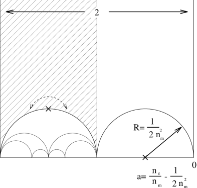
Figure 4: The strip of width 2 above the two largest arcs is the fundamental region of monodromy group $\Gamma(2)$ as found by the method of isometric cycles described in app. B. Its area is by (B.1) is $A=2\pi$ hence six times the one of $SL(2,\hbox{ZZ})$. Because of the identification (3.15) the fundamental region of the quantum symmetry  group of pure $SU(2)$ is given by the hatched region, which corresponds to the group $\Gamma_{0}(2)$, the subgroup of $SL(2,\hbox{ZZ})$ with $C=0\ {\rm mod}\ 2$. The marked point at $\tau_{0}=-3/2+i/2$ is the $Z_{2}$ orbifold point of $\Gamma_{0}(2)$, hence by (B.1) $A=\pi$. In particular the identification by the $T$ generator (2.3) $\tau\rightarrow\tau+1$ is realized in the $N=2$ theory, while the $S$ generator is not realized.

$\bullet$ The solutions:

Now if $n=3$ one can choose from the 10 redundant parameters in $Q$ as the free parameters in (3.32) the angles $\alpha_{i}$ and the uniformization problem is solved by the Schwartz-triangle functions, which are ratios of hyper geometric functions see e.g. [46]. This cases were completely studied in the last century, for general discrete subgroups of $SL(2,\hbox{IR})$. Especially if $\alpha_{1}=\alpha_{2}=\alpha_{3}=0$ as for our three necessarily parabolic elements the subgroup $\Gamma$ is uniquely determined, if the boundary conditions are obeyed. For pure ${\rm SU}(2)$ it is given by the index $6$ congruence subgroup denoted by $\Gamma(2)$, which is defined as in

$$\Gamma(N)=\left\{\left.\left(\matrix{A&B\cr C&D}\right)\in SL(2,\hbox{ZZ})\right|\matrix{&\!\!\!!\!\!B,C=0\,{\rm mod}\,N\cr&\!\!\!\!\!A,D=1\,{\rm mod}\,N}\right\}.$$

Alternatively one can argue that the pairs of massless dyons, which satisfy (3.31), are precisely $M^{\Lambda^{2}}_{(1,n)}$ $M^{-\Lambda^{2}}_{(1,n-1)}$$=M^{\infty}$. Any two of these matrices generate $\Gamma(2)$. The choice of $n$ corresponds to the $\theta$ shift symmetry, that is different choices correspond to the same physics, so we may chose $n=0$.

The linear differential equation (3.34) is equivalent, in the sense explained below, to the hyper geometric equation ${\cal L}f=0$ with

$${\cal L}=z(1-z){{\rm d}^{2}\over{\rm d}^{2}z}+[c-(a+b+1)z]{{\rm d}\over{\rm d}z}-ab$$ (3.36)

with parameters

$$a={1\over 2}(1+\alpha_{\infty}-\alpha_{0}-\alpha_{1}),\quad b={1\over 2}(1-\alpha_{\infty}-\alpha_{0}-\alpha_{1}),\quad c=1-\alpha_{0}\ .$$ (3.37)

Here by the indices on the $\alpha$ we indicate the associated singularities $z_{i}$ in (3.32), which have been fixed to be $0,1,\infty$. This differs from the choice we made in the $u$-plane $-\Lambda^{2},\Lambda^{2},\infty$. To check the parameter identification we note that a second order linear differential equation

$$\varpi^{\prime\prime}+p\varpi^{\prime}+q\varpi=0$$ (3.38)

can be brought to the form (3.34) by substitution of $f(z)=g(z)\varpi(z)$ with $g(z)=\exp-{1\over 2}\int^{z}pdz^{\prime}$. No matter how we write (3.38) by choosing a particular $g(z)$ the invariant quantity on which the definition of $\tau$ depends is

$$Q=q-{p^{\prime}\over 2}-{p^{2}\over 4}\ .$$ (3.39)

Using this definition of $Q$ it is easy to check from (3.32) with $\beta_{i}=0$ and (3.36) the parameter identification (3.37) for the triangle groups.

From the physics point of view there is distinguished form of (3.38) namely the one for which $g(u)$ in (3.35) is constant. As is turns out the hypergeometric equation with $a=b={1\over 2}$ $c=1$ is itself the preferred form. This can be easily seen by putting the singularities in (3.36) from $z=0,1$ to $u=\pm\Lambda^{2}$ by the substitution $z={1-u\over 2}$ which transforms it to ${\cal L}\vec{\varpi}=0$ with

$${\cal L}=\partial_{u}^{2}-{2u\partial_{u}\over\Lambda^{4}-u^{2}}-{1\over 4(\Lambda^{4}-u^{2})}$$ (3.40)

Now we can chose solutions $\varpi_{D},\varpi$, which lead to the correct leading behavior (3.26), (3.28) with constant $g$. Hence we can commute ${\cal L}\partial_{u}$ to $\partial_{u}{\widehat{\cal L}}$ so that $\vec{V}(u)$ is determined (the argument is up to additive constant, which has to be set to zero) by ${\widehat{\cal L}}\vec{V}=0$ with

$${\widehat{\cal L}}=\partial_{u}^{2}-{1\over 4(\Lambda^{4}-u^{2})}$$ (3.41)

This equation can be brought also in the hypergeometric form (3.36) with $(a,b,c)=(-{1\over 4},-{1\over 4},{1\over 2})$ by substituting $\alpha:=u^{2}/\Lambda^{4}$. Hence we get compact formulas for the physical $a_{D}(u),a(u)$, which determine the masses of the BPS states

$$\begin{array}[]{rl}a_{D}(\alpha)&=\displaystyle{{i\Lambda\over 4}(\alpha-1)\,_{2}F_{1}\left({3\over 4},{3\over 4},2;1-\alpha\right)}\\[8.53581pt] a(\alpha)&=\displaystyle{{\sqrt{2}\Lambda}\alpha^{1\over 4}\ _{2}F_{1}\left(-{1\over 4},{1\over 4},1;{1\over\alpha}\right)\ .}\end{array}$$ (3.42)

3.3 N=2 versus N=4 conventions

There exist two conventions of charge normalizations in the literature. In the $N=4$ conventions the smallest occuring electric charge, that of the $W^{+}$ boson, is set to one. Since one can add matter to $N=2$ theories the smallest charge is now that of the quarks and is set often to one in the $N=2$ conventions. There is no change in the magnetic charge units however. E.g. in $SU(2)$ the effect is that the $W$-bosons have charge $|2|$ in the $N=2$ units and to keep (3.5) one has to transform $(a_{D},a)\mapsto(a_{D},a/2)$, $\tau\mapsto 2\tau$ and conjugate the monodromies by

$$M\mapsto C^{-1}MC\ \ {\rm with}\ \ C=\left(\matrix{1&0\cr 0&2}\right)\ .$$ (3.43)

For pure $SU(2)$ the group $\Gamma_{M}$ generated by the monodromies in the new conventions becomes $\Gamma^{0}(4)$, which are the $SL(2,\hbox{ZZ})$ transformations with $B=0\ {\rm mod}\ 4$, instead of $\Gamma(2)$. Because of (3.15) the full quantum symmetry is in this case $\Gamma^{0}(2)$. As the $T$ shift of (2.3) is $\tau\mapsto\tau+2$ in the new conventions the $\Gamma^{0}(2)$ is not the canonical $\Gamma^{0}(2)$ subgroup of the $SL(2,\hbox{ZZ})$ S-duality group we started with. It is conjugated to the more canonical $\Gamma_{0}(2)$ by a (not physical) $S$ duality, in general $\Gamma^{0}(N)=S\Gamma_{0}(N)S^{-1}$. It is however the canonical subgroup $\Gamma^{0}(2)$ subgroup of the $SL(2,\hbox{ZZ})$ found for the other conformal theory with $N_{f}=4$ flavors see sect. (3.4). The fundamental regions for $\Gamma^{0}(2)\subset\Gamma^{0}(4)$ looks exactly as the fundamental regions $\Gamma_{0}(2)\subset\Gamma(2)$ depicted in the Fig.4 except that the whole figure is scaled such that the indicated width becomes $4$. Counterintuitively the scaling does not affect the hyperbolic areas as it is clear from formula (B.1), so the index of the groups in ${\rm SL}(2,\hbox{ZZ})$ does not change. Similar the fundamental region for $\Gamma_{0}(4)$ looks like the $\Gamma(2)$ area in Fig.4 when scaled to width $1$.

3.4 The symmetries on the dyon spectrum.

Let us investigate, purely from symmetry considerations, what states could be there. To discuss that it is useful to adopt the $N=2$ conventions and to think the groups $\Gamma\in{\rm SL}(2,\hbox{ZZ})$ as canonical subgroups of the $N_{f}=4$ ${\rm SL}(2,\hbox{ZZ})$. Bare masses of the quarks are set to zero in the following.

For $N_{f}=0$, there are no dyons with the smallest charge unit, so the possible states are $(n_{m},2n_{e})$ and the subgroup leaving them invariant is $\Gamma^{0}(2)$.

For $N_{f}>0$ the dyons can be labeled by their $2N_{f}$-fermion zero modes, which form after quantization a ${\rm Spin}(2N_{f})$ representation [2]. The elementary hyper multiplets transform in the vector representation of $SO(2N_{f})$, while monopoles (dyons) are in the spinor representation and as was pointed out in [2] they are in the different conjugacy classes $s$ or $c$ depending of whether they carry in addition even or odd electric charge.

For $N_{f}=2$ ${\rm Spin}(4)={\rm SU}(2)\times{\rm SU}(2)$ with center $Z_{2}\times Z_{2}$. That means that the transformation properties of a state $(n_{e},n_{m})$ w.r.t. the center must given by the $Z_{2}$ charges $((n_{e}+n_{m})\ {\rm mod}\ 2,n_{e}\ {\rm mod}\ 2)$. Especially states with $(n_{m},n_{e})=(2k+1,l)$ are spinor classes and should transform among themselves i.e. the $C$ in the $SL(2,\hbox{ZZ})$ transformation must be even, while $B$ can be $1$, this mixed $s$ and $c$ classes, but that is allowed because the corresponding outer isomorphism is realized in ${\rm SO}(4)$. That implies that the ${\rm SL}(2,\hbox{ZZ})$ is broken to $\Gamma_{0}(2)$.

For $N_{f}=3$ the center of ${\rm Spin}(6)=SU(4)$ is $Z_{4}$ and since vectors have charge $2$ the $Z_{4}$ must act as $\exp{2\pi i\over 4}(n_{m}+2n_{e})$ on dyons. In particular the vectors have charges $(n_{m},n_{e})=(4k,l)$ the spinors $(4k+1,l)$, $(4k+3,l)$ and the scalars $(4m+2,l)$, which means that $c=0\ {\rm mod}\ 4$ i.e. ${\rm SL}(2,\hbox{ZZ})$ must be broken to $\Gamma_{0}(4)$.

For $N_{f}=4$ the relevant ${\rm Spin}(8)$ has center $Z_{2}\times Z_{2}$ but the $Z_{2}$ charges are $o:(0,0)$, $v:=(0,1)$, $s:(1,0)$ and $c:(1,1)$. The $Z_{2}$ charges of dyons must be $(n_{m}\ {\rm mod}\ 2,n_{e}\ {\rm mod}\ 2)$. Now the minimal shifts $b=1$, $c=1$ of ${\rm SL}(2,\hbox{ZZ})$ permute the $v,s,c$ classes but that could still be a valid symmetry as ${\rm Spin}(8)$ allows for an outer automorphism called triality symmetry, which in fact permutes this classes by $S_{3}$. We can define a homomorphisms $h:SL(2,\hbox{ZZ})\rightarrow S_{3}$ by modding the matrix entries $A,B,C,D$ by $2$, so that the total symmetry group can be the semi direct product ${\rm Spin}(8)\mathbin{\hbox{\hskip 2.0pt\vrule height=5.0pt,depth=-0.3pt,width=0.25pt\hskip-1.6pt$\times$}}{\rm SL}(2,\hbox{ZZ})$.

If we accept these subgroups, we get the generating monodromies and the associated massless particles and solutions without further effort. We can read off generating monodromies from the fundamental region as they are the ones which conjugate the arcs of $F$ in pairs. Alternatively we may consider dyons with the smallest electric and magnetic charges, which generate according to (3.31) the symmetry $\Gamma_{M}$, which is up to the discrete symmetry (3.15,3.17) the quantum symmetry $\Gamma$. Note that in $N=2$ conventions one has to rescale $M_{(n_{m},n_{e})}$ of (3.30) we call the rescaled monodromy $\tilde{M}_{(n_{e},n_{m})}:=M_{({n_{m}\over\sqrt{2}},{n_{e}\over\sqrt{2}})}$. Let us summarize the quantum symmetry groups $\Gamma$, the monodromy groups and defining generators corresponding to the shortest massless dyon states for the cases in turn

$$\begin{array}[]{rl}N_{f}=0:&\Gamma^{0}(2):\ \Gamma^{0}(4):\tilde{M}_{(1,0)}\tilde{M}_{(1,-2)}=T_{0}\\[8.53581pt] N_{f}=2:&\Gamma_{0}(2):\ \Gamma(2):\ M_{(1,0)}M_{(1,-1)}=T_{2}\\[8.53581pt] N_{f}=3:&\Gamma_{0}(4):\ \Gamma_{0}(4):\ \tilde{M}_{(2,0)}\tilde{M}_{(2,-1)}=T_{3},\end{array}$$

Here the $(2,0)$ is expected according to section 2 not to be a stable monopole, but at best a bound state a threshold. $T_{N_{f}}$ is the semiclassical monodromy due to the $\beta$-function logarithm and the Weyl-reflection it is $T_{N_{f}}:=-(T^{N_{f}-4})$. $\tau(u)$ will be given by the Schwarz triangle function with appropriate boundary conditions and $a_{D}(u),a(u)$ can again be very simply obtained from solutions of hypergeometric functions. The situation for $N_{f}=4$ is in some sense the simplest as $\tau$ will not depend on $u$.

For $N_{f}=1$ we have (at least) four singularities because of the $Z_{3}$ symmetry and cannot expect such an extremely easy relation to the triangle functions of a subgroup of $SL(2,\hbox{ZZ})$. From the double scaling limit of the $N_{f}=4$ theory see (4.23) and the Lefshetz monodromy (compare the discussion in 4.3) one finds that the three monodromies are associated to the following massless particles $\tilde{M}_{(1,0)}\tilde{M}_{(1-1)}\tilde{M}_{(1,-2)}=T_{1}$.

3.5 Consistency checks:

$\bullet$ Consistency checks from instanton coefficients : This explicit solutions can of course be used to calculate ${\cal F}$ everywhere in the moduli space. For instance the first coefficients in (3.12) for pure ${\rm SU}(2)$ are given by

  $$n 1 2 3 4 5 6 {\cal F}_{n} {1\over 2^{2}} {5\over 2^{7}} {3\over 2^{7}} {1469\over 2^{16}} {4471\over 2^{15}\cdot 5} {40397\over 2^{20}}$$                                         

The function

$$\begin{array}[]{rl}{\cal G}:=&{i\pi\over 2}\int(a_{D}{\rm d}a-a{\rm d}a_{D})\cr=&i\pi({\cal F}-{1\over 2}a\dot{\cal F})\ ,\end{array}$$ (3.44)

with $\dot{}:={{\rm d}\over{\rm d}a}$, is obviously modular invariant. It is easy to see that ${\cal G}$ behaves at the cusps like $u$ since it is modular it must be therefore that ${\cal G}=u+const.$ and the constant is zero as one can see from the vanishing of ${\cal G}$ at $u=0$. It was later shown in [49] from the $N=2$ Ward-identities that ${\cal G}={\rm Tr}({\langle}\phi^{2}{\rangle})$, which justifies the assumption that ${\rm Tr}({\langle}\phi^{2}{\rangle})$ is the good variable in the moduli space. Note furthermore that, because of ${\cal F}=a^{2}f(a/\Lambda)$ and using ${\cal G}=u$ we get

$$\Lambda{{\rm d}\over{\rm d}\Lambda}F=-{i\over\pi}u.$$ (3.45)

Now transforming the dependent variable in (3.41) from $u\rightarrow a(u)$ and using ${\cal G}=u$ and the fact that $a(u),a_{D}$ is a solution one gets [48] a differential equation for ${\cal G}$

$$(1-{\cal G}^{2})\ddot{\cal G}+{1\over 4}a\dot{\cal G}^{3}=0$$ (3.46)

and the same equation for the analogous defined ${\cal G}_{D}$. From (3.46) one can derive a recursion relation for the instantons coefficients, which can be found in [48].

Eq. (3.46) governs the non-perturbative effects in the strong and the weak coupling region, it should in principle be understandable directly from explicit non-perturbative calculations. At least ratios of the instantons coefficients have been successfully compared for $SU(2)$ with $N_{f}<4$ in [51] by a very tedious direct calculation. This is a certainly very encouraging independent check for the solutions,

$\bullet$ Consistency checks from the dyon spectrum

The consistency checks on the dyon spectrum for $N_{f}=4$ are quite similar to the $N=4$ case. $\tau$ does not depend on $u$ and once $\tau$ is generically fixed the lattice spanned by, say normalized vectors, $1$ and $\tau$ is non degenerate and one has to check that bound states of the stable dyons for which $(n_{e},n_{m})$ is coprime exist, since they must be present in theory as they occur in the ${\rm SL}(2,\hbox{ZZ})$ orbit (on which the ${\rm Spin}(8)$ representations are mixed) of e.g. the stable $(0,1)$ electron.

For $N_{f}<4$ the lattice, spanned by $a_{D}(u)$ and $a(u)$, is $u$ dependent and degenerates at a subspace $K:=\{p\in{\cal K}|{\rm Im}(k(p))=0\}$ in the moduli space, where we define $k(u):=a_{D}(u)/a(u)$. $K$ is called curve of marginal stability. It was known for $N_{f}=0$ that beside the elementary electrically charged particles only configurations for the monodromy generating states and their $\theta$-shifted companions, i.e $(1,n)$ ($N=4$ conventions) exist semiclassically. That turns out to be a general feature and the nontrivial prediction concerning new dyons are the existence of the $(2,n)$ bound states with $n$ odd in the $N_{f}=3$ theory [2], which were found in fact later [34].

On the other hand it is an internal consistency check that the monodromy generating dyons are the only magnetically charged states in the spectrum at semiclassical infinity. For that to work the topology of the set $K$ must be such that the existing dyons and elementary particles cannot be transformed by a monodromy loop in the $u$-plane into unwanted states and continued to the semiclassical region without encountering a point on $K$, where all unwanted states can decay. From (3.5) it is clear that that $k(u_{s})={a_{D}(u_{s})\over a(u_{s})}=-{n_{e}\over n_{m}}$ is rational at the singularity $u_{s}$ due to the massless dyon $(n_{m},n_{e})$. So by construction $K$ contains these singularities. If $K$ exists outside the singular set it must be there a continuous codimension one subspace. That is easy to see, because $a,a_{D}$ are holomorphic, so $k$ is a harmonic function outside the singularities and ${\rm d}k=0$ would imply that the Hessian vanishes, but the Hessian of $k$ is proportional to ${\rm Im}\,\tau$ and can vanish only at the singularities, compare Fig.4. Now because of the $a_{V}$ term in (3.28) ${\rm d}k\neq 0$ also at the singularities, so that $K=0$ is a smooth real codimension one curve everywhere. Note again the importance of the $a_{V}\neq 0$ constant, if it were not present the ${\rm Im}\,k=0$ subset would be stuck at the singularities as the ${\rm Im}\,\tau=0$ “curve” in fact is.

Let us discuss e.g. the situation for ${\rm SU}(2)$ with $N_{f}=0$ in the $N=4$ conventions. The up to the $T$-shift closed path in the complex $k$ plane runs from $k(u=-\Lambda^{2})=-1$, at which the $(1,1)$ dyon is massless, along the real axis to $k(u=\Lambda^{2})=0$, at which the $(1,0)$ state is massless, to the $k(u=-\Lambda^{2})=1$, at which the $(1,-1)$ state is massless, must therefore have a smooth pre-image in the $u$-plane. Hence $K$ has the right topology. Note that the values of $k(u)$ at $u=\pm\Lambda^{2}$ depend really on the strip $R_{\infty}$ we have chosen in Fig.4.

Besides the aspect that certain states can decay on $K$ there is a second important aspect related to the existence of $K$, which has been used [52] to construct the spectrum in the weak and the strong coupling region. No other states than the dyons $(1,n)$, which are responsible for the monodromies should become massless at $K$. More precisely the existence of a stable dyon with coprime integers $(n_{m},n_{e})\neq(1,n)$ in a region of the moduli space, which can be connected (without crossing $K$) to a point on $K$ on which it would become massless is forbidden. It would lead to an additional singularity incompatible with the actual solutions. Since ${\rm Re}\,k(u)$ takes a continuous set of real values this restricts the possible stable dyons drastically. The argument is facilitated by working with the parameter which labels truly inequivalent vacua, namely $\alpha=u^{2}/\Lambda^{4}$. This parameterization identifies the $(1,0)$ monopole singularity at $u=\Lambda^{2}$ and the $(1,-1)$ dyon singularity at $u=-\Lambda^{2}$, as it should, and creates an $\hbox{ZZ}_{2}$ singularity at the origin, which corresponds to the $\hbox{ZZ}_{2}$ fixpoint in fundamental region of $\Gamma_{0}(2)$. The monodromies can easily worked out from the solution (3.42). As expected they contain phases $\rho$ with $\rho^{4}=1$ corresponding to the $\hbox{ZZ}_{4}$-action on $\vec{V}$. The action on $\tau$ is generated by $M^{\infty}=\left(\matrix{-1&1\cr 0&-1}\right)$, $M^{1}=\left(\matrix{1&0\cr-2&1}\right)$ and $M^{0}=\left(\matrix{1&1\cr-2&-1}\right)$ with $M^{0}M^{1}=M^{\infty}$ and on $(n_{m},n_{e})^{t}$ it acts by $(n_{m},n_{e})^{t}\mapsto(M^{-1})^{t}(n_{m},n_{e})^{t}$.

Figure 5: The vector moduli space of $N_{f}=0$ ${\rm SU}(2)$ theory is parameterized by $\alpha=u^{2}/\Lambda^{4}$ and compactified to a sphere. $K$ divides the sphere into the strong coupling region containing $\alpha=0$ and the weak coupling region containing $\alpha=\infty$. On $K$ ${\rm Re}\ k(\alpha)$ runs continuously from $0$ at $\alpha=1$ to $1$ at $\alpha=1$. Note that there are branch cuts running along $\overline{0,1}$ and along $\overline{1,\infty}$.

From Fig.5 we see that the $\alpha$-sphere is divided by $K$ into two regions.

$\bullet$ The weak coupling spectrum: The region at infinity is governed by the $M^{\infty}$ monodromy. By this monodromy a stable state with $|n_{m}|>1$ can be converted into one for which $-n_{e}/n_{m}\in[0,1]$ hence all these states are forbidden. Beside the $(1,n)$ dyons and their antiparticles the $W^{\pm}$ bosons with $(0,\pm 1)$ are of course also allowed as they are stable under the $M^{\infty}$ action and do not become massless at $K$.

$\bullet$ The strong coupling spectrum: Now we ask again for the states $(n_{m},n_{e})$ for which $-n_{e}/n_{m}$ cannot be brought by the $M^{0}$ action into the interval $[0,1]$. The conclusion is that for our choice of the strip $R_{\infty}$ this strong coupling spectrum consists only of the massless monopole $(1,0)$ and its antiparticle.

$\bullet$ This picture predicts in particular at $K$ the decay of the charged vector multiplet of the $W^{\pm}$ $(0,\pm 1)$ boson into two hyper multiplets of magnetic monopoles $(-1,\pm 1)$ and $(1,0)$, which is possible from mass by charge and conservation, if $a_{D}/a\in[0,1]$. Note that the $(-1,\pm 1)$ state is identified by the $(M^{0})^{\pm}$ monodromy with the $(-1,0)$ state.

Finally convincing evidence for the consistency of Seiberg-Witten solutions come from the connectedness of these theories via limits in the quarks masses. Starting from massive $N_{F}=4$ one gets indeed every other theory, by sending part of the quark masses to infinity, see the discussion above (4.23). Such arguments apply also to the higher rank groups and can be best discussed in the geometrical picture to which we turn now.

4 The geometrical picture :

4.1 General ideas

We have seen in (3.40,3.41) that there were differential equations completely adapted the problem of finding the exact BPS masses and the exact gauge coupling. Were do this equations come from ? In context of the uniformization problem it was already observed by [39] that e.g. (3.40) is the Picard-Fuchs equation fulfilled by the period integrals of a specially parameterization family of an elliptic curves ${\cal E}(u)$. In particular the solutions $\varpi_{D}$ and $\varpi$, which solve the uniformization problem

$$\tau(u)={\varpi_{D}(u)\over\varpi(u)}\$$ (4.1)

correspond to the integrals of the holomorphic differential $\omega$ (4.14) over homology cycles which generate $H^{1}({\cal E},\hbox{ZZ})$, i.e.

$$(\varpi_{D}(u),\varpi(u))=(\oint_{B}\omega,\oint_{A}\omega)\ .$$ (4.2)

That is not very surprising as the maximal discontinuous reparametrization group of the torus is ${\rm SL}(2,\hbox{ZZ})$ and if we insist to stay within a parameterization family, which obeys some additional finite symmetries the ${\rm SL}(2,\hbox{ZZ})$ will broken down to a subgroup of finite index in ${\rm SL}(2,\hbox{ZZ})$ just like e.g. $\Gamma(2)$. Moreover if one finds a form $\lambda$ such that the integrals $\oint_{\gamma}\lambda$ are well defined for $C\in H^{1}({\cal E},\hbox{ZZ})$ and

$$\partial_{u}\lambda=\omega+{\rm exact\ form}$$ (4.3)

then we find from (3.24)

$$(a_{D}(u),a(u))=(\oint_{B}\lambda,\oint_{A}\lambda)\ .$$ (4.4)

From the above requirements it is clear that

a.) $\lambda$ is a meromorphic form, as the holomorphic form is unique, but with

b.) vanishing residues as otherwise the integral would depend on the path.

In the cases with non-zero masses condition b.) is too strong. In fact the shift by $H$ in (3.25) has the explanation that one picks up a contribution from the residue, if the cycle defining $a_{D}(u),a(u)$ undergoes a Lefshetz monodromy.

Figure 6: A scetch of the identification of the electro-magnetic charge lattice with the independent cycles of the torus

Eq. (4.4) defines an identification of the electro-magnetic charge lattice $\Lambda$ Fig.1 with the lattice of integral homology $H_{1}({\cal E},\hbox{ZZ})$.

$$\phi:\Lambda\rightarrow H^{1}({\cal E},\hbox{ZZ})\ .$$ (4.5)

By the symmetries of the problem the identification can be made in various ways, e.g. for the scale invariant theories (4.5) is actually up to ${\rm SL}(2,\hbox{ZZ})$ reflecting electro-magnetic duality. For the scale dependent families ${\cal E}(u)$ the ambiguity is reduced to a subgroup of $SL(2,\hbox{ZZ})$. That comes essentially because we have to identify the particles, which become massless, with the vanishing cycles of the family. Another choice which was made in (4.4) was the orientation of the cycles. Reversing globally the orientation correspond to the exchange of particles and antiparticles.

$\bullet$ Positivity of the metric and Riemann bilinear relations:

A very nice feature of this geometric interpretation is that ${\rm Im}(\tau)$ is the normalized volume of the torus, so positivity of the metric is guaranteed by construction. Let us see how this is derived and how it generalizes to guarantee positivity of the metric (3.23) as obtained from the periods of a general Riemann surface $X$. One a even dimensional manifold of real dimension ${\rm dim}=2r$ with $r$ odd and $2k={\rm rank}(H^{r}(X,\hbox{ZZ}))$ one can always chose a symplectic basis $A^{i}$, $B_{i}$ $i=1,\ldots,k$ of $H_{r}(X,\hbox{ZZ})$ i.e. with the intersection pairing

$$\begin{array}[]{rl}A^{i}\cap A^{j}&=B_{i}\cap B_{j}=0\cr A^{i}\cap B_{j}&=(-)^{r}B_{j}\cap A^{i}=\delta^{i}_{j}\ .\end{array}$$ (4.6)

For our Riemann surfaces and the threefold CY we discuss later this choice is up to ${\rm SP}(2k,\hbox{ZZ})$. If $r$ is even there will be a nontrivial signature associated to the bilinear pairing (4.6), which we will calculate in section 5.1 .

By Poincaré duality we can also chose a topological basis for $H^{r}(X,\hbox{ZZ})$ $\alpha_{i}$, $\beta^{i}$ $i=1,\ldots,k$ with the following properties

$$\begin{array}[]{rl}\int_{X}\alpha_{i}\wedge\alpha_{j}&=\int_{X}\beta^{i}\wedge\beta^{j}=0\\[8.53581pt] \int_{X}\alpha_{i}\wedge\beta^{j}&=(-)^{r}\int_{X}\beta^{j}\wedge\alpha_{i}=\delta^{j}_{i}\\[8.53581pt] \int_{A^{j}}\beta^{i}&=\int_{B_{j}}\alpha_{i}=0\\[8.53581pt] \int_{A^{j}}\alpha_{i}&=\delta^{j}_{i},\ \ \int_{B_{j}}\beta^{i}=\delta^{i}_{j}\ .\end{array}$$ (4.7)

The topological basis we fix according to a given choice of topological cycles and it will not be holomorphic w.r.t. to the complex structure, which varies with the moduli. Using the moduli dependent basis of holomorphic forms $(1,0)$ on a Riemann surface: $\omega_{i}$ $i=1,\ldots,k$ (4.38) and the $(k,2k)$ period matrix

$$({\bf W_{D}}_{ji},{\bf W}_{ji}):=\left(\int_{B_{i}}\omega_{j},\int_{A^{i}}\omega_{j}\right)$$ (4.8)

the definition of $\tau$ from (4.1,4.2) can be generalized to ${\bf T}={\bf W}^{-1}{\bf W_{D}}$. In fact first for $g=1$ we get with (4.14) $i\int_{X}\omega\wedge\bar{\omega}=i\int_{X}dz\wedge d{\bar{z}}=2\int_{X}dx\wedge dy=2\,{\rm vol}(X)$ and on the other hand by developing $\omega$ and $\bar{\omega}$ in the basis $\alpha,\beta$, i.e. $\omega=\varpi_{D}\beta+\varpi\alpha$, we get $i\int_{X}\omega\wedge\bar{\omega}=i\varpi[\bar{\tau}-\tau]\bar{\varpi}=2|\varpi|^{2}{\rm Im}(\tau)$, hence ${\rm Im}(\tau)>0$. By considering all bilinear pairings between $\omega_{i}$ and $\bar{\omega}_{j}$ as well as between $\omega_{i}$ and $\omega_{j}$ one gets a straightforward generalization to higher genus [79] which yields the first and second Riemann bilinear relation:

$$\begin{array}[]{rl}{\bf T}-{\bf T}^{t}&=0\cr{\rm Im}[{\bf T}]&>0\ .\end{array}$$ (4.9)

Also the identification (4.5) generalized immediately to higher rank lattices $\Lambda$ and general Riemann surfaces $X$. The electro-magnetic charge lattice $\Lambda$ with $H_{1}(X,\hbox{ZZ})$ maps the generalization of the symplectic bilinear form (2.6) to the intersection form (7.7). Once the choice (7.7) has made states with only electric charge quantum numbers will be identified with one sort of cycles, say the $A$-cycles, and purely magnetically charged must then be identified with the $B$ cycles. Now, if we have a special parametrisation family with $k$ deformations $u_{i+1}$ $i=1,\ldots,k$ and have identified a meromorphic form $\lambda$ with $\omega_{i}=\partial_{u_{i+1}}\lambda+{\rm exact\ form}$ and $a_{D}^{i}=\oint_{B_{i}}\lambda$, $a^{i}=\oint_{A_{i}}\lambda$ then the positivity of the metric ${\rm Im}[{\bf T}_{ij}]={\rm Im}[\partial_{a_{i}}a^{j}_{D}]$ in every direction in field space is guaranteed from ${\rm Im}[{\bf T}]>0$, while the integration condition for the existence of ${\cal F}$ with $a_{D}^{i}=\partial_{a_{i}}{\cal F}$ is ${\bf T}-{\bf T}^{t}=0$ !

$\bullet$ Lefshetz formula and one loop $\beta$-function:

This makes Riemann surfaces candidates whose periods can describe the effective action of theories with higher rank gauge groups. The task is then to find parameterization families of Riemann surfaces, which have the right discrete symmetries and give the right monodromies. The monodromies of algebraic varieties on the middle homology $H_{r}(X,\hbox{ZZ})$ are determined by the cycles which shrink to zero volume at the singular degenerations of the variety. These are called the vanishing cycles. More precisely the Lefshetz formula gives the monodromy action on an arbitrary cycle $C\in H_{r}(X,\hbox{ZZ})$ along a path in the moduli space around a complex codimension one locus, where one cycle $V\in H_{r}(X,\hbox{ZZ})$ vanishes as

$$M_{V}:C\mapsto C+(-1)^{(r+1)(r+2)/2}n(C\cap V)V\ ,$$ (4.10)

Here the integer $n$ depends on the local parameterization of the singularity by the moduli, which is forced to us from the family (see below). In singularity theory the parameterization is chosen such that $n=1$.

In the simplest cases the vanishing cycle has the topology of an $S^{r}$ and its self intersection number is $(V\cap V)=(-1)^{r(r-1)/2}(1+(-1)^{r})$ ( [109], Lemma 1.4). In particular for $r$ odd, we get then a physical interpretation of (4.10) as a shift from the one-loop $\beta$-function as in the discussion below. For $r$ even on the other hand (4.10) is a reflection in $H_{r}(X)$ on the hyperplane perpendicular to $V\in H_{r}(X)$, which is just a Weyl-reflection, if the intersection pairing is proportional to the Cartan matrix as in the zero dimensional example (4.31) and on $K3$ surfaces [82].

Up to phase factors, which can come from the forms $\lambda$ (or $\omega$) eq. (4.10) describes also the monodromies on the period vectors $\vec{V}$ (or $\vec{\varpi}$). In view of the map (4.5) one might ask, which states are mapped to these vanishing cycles and what is the local physics associated to the monodromy. For the most generic singularity, where precisely one cycle shrinks to zero as above, the answer is simple. The period $a_{V}:=\oint_{V}\lambda$ is proportional to the mass of the light charged particle $\Phi_{V}$ (and its antiparticle) which sets the infrared cut off in (3.6). The ratio between the mass of this particle $\Phi_{V}$ and its magnetic (or electrical) dual particle will be zero at the singularity. After a basis transformation which diagonalizes ${\bf T}$ we calculate the gauge coupling of the gauge boson(s), which couple locally to $\Phi_{V}$. From (3.1) we get $\tau_{V}\propto\kappa\log(a_{V})+{holomorphic}$ and the period dual to $a_{V}$ will be therefore $a_{D}^{V}=\oint_{V_{D}}\lambda\propto\kappa a_{V}\log(a_{V})+holomorphic$. This gives rise in the new basis rise to a shift, which corresponds in the old basis to (4.10). If $\lambda$ is regular at the degeneration, as it turns out to be the case for singularities due to magnetically charged states, the mass of the particle will actually go to zero. The Lefshetz theorem is quite useful to make consistency checks on the curves for the higher rank gauge groups [53].

In type IIB string theory an analogous picture arises, when a single cycle in the middle homology of a CY shrinks to a point [6] [172]. The wrapping of a $D$-3-brane around the vanishing 3-cycle leads to an object which looks from the four dimensional point of view like a black-hole. By (6.21) its mass is proportional to the volume of the vanishing cycle. In particular at the degeneration point $a_{V}=0$ this particle cannot be integrated out, but has to be included in the Wilsonian supergravity action, just as in the rigid case the magnetic monopole. Very similarly it produces an one-loop $\beta$ function logarithm in the coupling of the dual gauge field, which gives rise to the shift in (4.10).

$\bullet$ Variants of the idea: The columns of the period matrix (4.8) define a lattice $\Lambda_{X}$ from which the Jacobian variety of the genus $g$ Riemann surface is constructed as ${\cal J}(X)=\,\hbox{IC}^{g}/\Lambda_{X}$. There is a natural generalization in which one imposes the condition (4.9) on arbitrary non degenerate rank $r$ lattices $\Lambda^{a}$. The quotients $\,\hbox{IC}^{r}/\Lambda^{a}$ with this restriction are known as abelian varieties [79]. If the abelian variety has complex dimension greater then two, it is not necessarily the Jacobian variety of a Riemann surface. In physics context mainly Jacobian and Prym varieties occur. In the later cases the Riemann surface admits an automorphism, so that periods get identified and the abelian variety is defined from the quotient of the period lattice. In fact in this way one can define infinitely many Riemann surfaces of different genus, which describe the same gauge group. Cases which have no geometrical interpretation from a Riemann surface seem rare, comp. sect. (4.4.2).

While there were probably no consistent $N=2$ theories in 4d before the work of Seiberg-Witten, one can satisfy at least the basic consistency requirements with a Riemann surface, which admits a differential form $\lambda$ and gives rise to structure, like in (4.4). General theorems about the degeneration of the periods integrals imply that there are always local coordinates in the moduli space so that the the periods degenerate no worse then with a logarithmic singularity at the discriminate such that the effective action can always be determined (comp. section (4.2)). This may lead to the discovery of interesting exotic $N=2$ theories in four dimensions.

4.2 The curves for ${\rm SU}(2)$.

We will now discuss examples of Riemann surfaces, which correspond to gauge groups (with matter). I.e. the necessary discrete symmetries are realized and the periods have the prescribed physical monodromies and the right asymptotic behavior. For $SL(2,\hbox{ZZ})$ and the subgroups $\Gamma^{0}(N)$ and $\Gamma_{0}(N)$ the corresponding families of elliptic have been partly constructed long time ago in the context of the uniformization problem. Their periods are hence, comp. sect. (3.2.1), related to hypergeometric functions of type ${}_{2}F_{1}$. It is clear by the geometric ansatz and completely compatible with physics that the periods will always be Fuchsian functions [63] [38]. E.g. for pure $SU(3)$ the holomorphic periods where found [47] to fulfill Appells [64] [46] Vol. I $F_{4}({1\over 3},{1\over 3},{2\over 3},{1\over 2},4{u_{2}^{3}\over 27\Lambda^{6}},{u_{3}^{2}\over\Lambda^{6}})$ system and the $a^{i}$, $a_{D}^{i}$ periods fullfil Appells $F_{4}({1\over 6},{1\over 6},{1\over 3},{1\over 2},4{u_{2}^{3}\over 27\Lambda^{6}},{u_{3}^{2}\over\Lambda^{6}})$ system (see (4.29,4.34) for the definition of $u_{i}$), but in contrast to the ${\rm SL}(2,\hbox{ZZ})$ case the functions are in general not known.

4.2.1 Algebraic form of the torus:

Let us shortly review how the algebraic description of the torus arises [60] [59]. Define the torus in the standard form $T=\hbox{IH}/\Lambda$, were $\Lambda$ is spanned by the periods $\varpi_{1}$ and $\varpi_{2}$. I.e. $T$ is the fundamental cell of $\Lambda$ identified (orientation preserving) on opposite sides. We might normalize the periods such that the lattice is spanned by $\pi\tau$ with $Im(\tau)>0$ and $\pi$. Now we want to map $T$ into a set given by an algebraic constraint. To do this one needs first well defined functions on $T$, i.e. $f(z)=f(z+\pi)=f(z+\pi\tau)$ for $z\in\hbox{IH}$. The Weierstrass function

$$\wp(z,\tau)={1\over z^{2}}+\sum_{\omega\in\Lambda\setminus\{0\}}\left({1\over(z-\omega)^{2}}-{1\over\omega^{2}}\right)$$ (4.11)

has this property. It is easy to see that it converges in $T$, but has poles on the lattice sites. Moreover $\wp$ fulfills the differential equation

$$\left({{\rm d}\over{\rm d}z}\wp\right)^{2}=4\wp^{3}-g_{2}\wp-g_{3}$$ (4.12)

with $g_{2}(\tau)=60\sum_{\omega\in\Lambda\setminus\{0\}}{1\over\omega^{4}}=2/3^{2}E_{4}(\tau)$ and $g_{3}(\tau)=140\sum_{\omega\in\Lambda\setminus\{0\}}{1\over\omega^{6}}=(2/3)^{3}E_{6}(\tau)$. By identifying $x=\wp(z),y={{\rm d}\over{\rm d}z}\wp(z)$ every point $z$ in $T$ is mapped to a point on the algebraic constraint in $\,\hbox{IC}^{2}$

$$y^{2}=4x^{3}-g_{2}x-g_{3}\ .$$ (4.13)

This is true apart from the lattice points on $T$, which are mapped to infinity in the $x,y$-plane. This must be rectified by compactifying the latter to an $\hbox{IP}^{2}$. As it is clear from the construction the holomorphic differential $\omega:={\rm d}z$ can be written as

$${{\rm d}z={{\rm d}x\over y}}$$ (4.14)

and gives by integration over the cycles just the normalized period vector $(\pi,\pi\tau)$.

$E_{4}$ and $E_{6}$ are known as Eisenstein series, which are normalized so that they have a nice $q:=\exp(2\pi i\tau)$ expansion

$$\begin{array}[]{rl}E_{4}(\tau)&=1+240\sum_{n=1}^{\infty}{n^{3}q^{n}\over 1-q^{n}}\\[8.53581pt] E_{6}(\tau)&=1-504\sum_{n=1}^{\infty}{n^{5}q^{n}\over 1-q^{n}\,.}\end{array}$$ (4.15)

They are the, up to multiplication, unique automorphic (or modular) functions of weight $4$ and $6$, i.e. $E_{2k}({A\tau+B\over C\tau+D})=(C\tau+B)^{-2k}E_{2k}(\tau)$, which are holomorphic in the whole upper half-plane IH. Every modular function with this holomorphicity property and weight $2k$ can be written as degree $2k$ weighted polynom in $E_{4}$ and $E_{6}$ (or $g_{2}$ and $g_{3}$ of course). $E_{4}$ has simple zero at $\tau=i$ and $E_{6}$ at $\tau=\exp(2\pi i/3)$. The value at infinity is $g_{2}(i\infty)={120\over\pi^{4}}\zeta(4)=2^{2}/3$ and $g_{3}(i\infty)={280\over\pi^{6}}\zeta(6)=(2/3)^{3}$. So the combination with lowest modular weight, which has a simple zero at infinity is $g_{2}^{3}-27g_{3}^{2}=2^{12}\eta^{24}$ proportional to the 24th power of the Dedekind $\eta$-function, which has product representation $\eta:=q^{1\over 24}\prod_{n=1}^{\infty}(1-q^{n})$. The $j(\tau)$ function is the unique modular invariant function with a simple pole at infinity

$$J(\tau)={g_{2}^{3}\over\Delta}\ {\rm where}\ \Delta=g_{2}^{3}-27g_{3}^{2}$$ (4.16)

is the discriminant of the elliptic curve. Up to a factor $1728$ it has an integral expansion

$$j(\tau)=1728J(\tau)={E_{4}^{3}\over\eta^{24}}={1\over q}+744+196884q+21493760q^{2}+\ldots$$ (4.17)

In the following we will see $j$ frequently as a function of the specific parameter $u$ of the parameterization family ${\cal E}(u)$. In this case the identification $j(u)=j(\tau)$ will give us an invariant characterization of the family ${\cal E}(u)$! A similar theory for the modular functions of higher genus Riemann surfaces is discussed e.g. in [61].

$\bullet$ Universal Picard-Fuchs equation:

The integrals

$$\varpi_{C}=\oint_{C}\omega=\oint{{\rm d}x\over\sqrt{4x^{3}-g_{2}(u)x-g_{3}(u)}},$$

with contours $C$ as in Fig.7, called elliptic integrals; they are not elementary. Instead of direct integration, which can be done only after expanding the integrand, one can derive a differential equation for them. This is done by deriving a differential operator with the property ${\cal L}(u){{\rm d}x\over y}={\partial f\over\partial x}{\rm d}x$. As $C$ is closed ${\cal L}(u)\varpi_{C}=0$ and since there are only two independent solutions corresponding to the two independent integrals over $A$ and $B$ cycles a second order ${\cal L}(u)$ must exist. Such differential equations are called Picard-Fuchs equations. We explain in Appendix C two ways how the Picard-Fuchs equations can be derived.

To appreciate the rôle of the $j$-invariant and link the discussion here to the one in section (3.2), note that every elliptic curve with an arbitrary parameterization $s$ can be brought in the form (4.13), see footnote 25, and the Picard-Fuchs equation can then be written in the useful universal form

$$\begin{array}[]{rl}&\varpi^{\prime\prime}+p\varpi^{\prime}+q\varpi=0\quad{\rm with}\\[8.53581pt] p&=-\log^{\prime}({3\over 2\Delta}(2g_{2}g_{3}^{\prime}-3g_{2}^{\prime}g_{3})),\\[5.69054pt] q&={1\over 12}(p\log^{\prime}\Delta+\log^{\prime\prime}\Delta)-{1\over 16}(g_{2}(g_{2}^{2})^{\prime}-12(g_{3}^{2})^{\prime})\ ,\end{array}$$ (4.18)

where ${}^{\prime}={{\rm d}\over{\rm d}s}$.

If one now changes the coordinate $s\rightarrow J=j/1728$ one gets an universal Picard-Fuchs equation for the rescaled periods $\Omega=\sqrt{g_{2}\over g_{3}}\varpi$ depending only on $J$, see e.g. [160] and an universal expression for

$$Q=\left({3\over 16(1-J)^{2}}+{2\over 9J^{2}}+{23\over 144J(1-J)}\right)\ ,$$ (4.19)

which we recognize after a short calculation as the $Q$ appearing in the Schwarzian differential equation (3.32) for $\alpha_{0}={1\over 3}$, $\alpha_{1}={1\over 2}$ and $\alpha_{\infty}=0$. I.e. $j(\tau)$ is the inverse of the developing map for $SL(2,\hbox{ZZ})$ itself.

$\bullet$ The $N=4$ and $N=2$ $N_{f}=4$ curves: The tori for the scale invariant theories are expected from the sections (2) and (3.4) to exhibit exact ${\rm SL}(2,\hbox{ZZ})$ invariance. Therefore they should parameterized by the $u$ independent parameter $\tau$, that is (4.13) with $g_{2}(\tau)$ and $g_{3}(\tau)$ is in principle the correct form. In view of (2.1, 3.5) $a_{D},a$ depends however on $u$

$$\begin{array}[]{rl}a_{D}=&\tau a\cr a=&\left\{\begin{array}[]{rl}{1\over 2}\sqrt{2u}&{\rm for}\ N_{f}=4\cr\sqrt{2u}&{\rm for}\ N=4\end{array}\right.\end{array}$$ (4.20)

Because of (3.35) this implies that $\vec{\varpi}={\cal N}\sqrt{2/u}(\tau,1)^{t}$ with ${\cal N}=1/4$ for $N_{f}=4$ and ${\cal N}=1/2$ for $N=4$. We can rescale $dz\rightarrow{\cal N}\sqrt{2/u}dz$ to get that. For later comparisons in scaling limits one wants to work always with the standard $(1,0)$ form ${\rm d}z={\rm d}x/y$. So one rescales in addition $x\rightarrow x/u$ and $y\rightarrow{yu^{-{3\over 2}}/2}$. This leads to an $u$ dependent form of the curve

$$y^{2}=x^{3}-{1\over 4}g_{2}(\tau)xu^{2}-{1\over 4}g_{3}(\tau)u^{3},$$ (4.21)

while the $(1,0)$ form is transformed back to the standard one. The left hand side of (4.21) can be factorized $y^{2}=\prod_{i=1}^{3}(x-e_{i}(\tau)u)$, where the zeros are given by the Jacobian Theta functions [59] $e_{1}(\tau)-e_{2}(\tau)=\theta_{3}^{4}(\tau)$, $e_{3}(\tau)-e_{2}(\tau)=\theta_{2}^{4}(\tau)$, $e_{1}(\tau)-e_{3}(\tau)=\theta_{4}^{4}(\tau)$.

$\bullet$ The $N=2$, $N_{f}\leq 4$ curves:

It was explained in [2] how to use the global ${\rm SO}(8)$ symmetry acting on the quarks to incorporate the bare masses into (4.21). An alternative derivation using the constraint on the residua of $\lambda$ form the inhomogeneous transformation law in (3.25) was also given in [2]. A particular nice representation of the corresponding curve was found in [55]

$$y^{2}=(x^{2}-u)^{2}-4h(h+1)\prod_{i=1}^{4}(x-m_{i}-2h\mu)$$ (4.22)

with $h={\theta_{2}^{4}\over\theta_{4}^{3}-\theta_{2}^{4}}$, $\mu={1\over N_{f}}\sum_{i=1}^{4}m_{i}$ and

$$\lambda={x-2h\mu\over 2\pi i}{\rm d}{\rm log}\left(x^{2}-u-y\over x^{2}-u+y\right)\ .$$

The curves for the asymptotic free $N_{f}<4$ theories can be obtained from (4.22) by considering the double scaling limit in which $M\rightarrow\infty$ and $\tau\rightarrow i\infty$ such that $\Lambda^{4-N_{f}}:=64\sqrt{q}M^{4-N_{f}}$ defines the finite scale of the $N_{f}<4$ theory. The leading terms of $\theta^{4}$ functions are $\theta_{2}^{4}=16q^{1/2}+{\cal O}(q^{3/2})$, $\theta_{3}^{4}=1+8q^{1/2}+{\cal O}(q)$, $\theta_{4}^{4}=1-8q^{1/2}+{\cal O}(q)$. With this one gets for the $N_{f}=0,\ldots,3$ cases the curves

$$y^{2}=(x^{2}-u)^{2}-\Lambda^{4-N_{f}}\prod_{i=1}^{N_{f}}(x+m_{i})$$ (4.23)

To show the equivalence of these curves with the ones in [2] we check that the $j$-invariants for $N_{f}=0,1$ are identical with ones of the corresponding curves in [2]. For the others a shift in the origin of $u$ is required e.g. for $N_{f}=2$ $u\rightarrow u-\Lambda^{2}/8$. Because of the absence of the a symmetry in the $u$-plane there is an unfixed shift in $u$ for the $N_{f}=3$ curve. The last reference in [51] suggest another choice of the shift then [2]. E.g. with (4.18) or the formalism in appendix C one can easily obtain the Picard-Fuchs equations for $\oint\omega$ and $\oint\lambda$ and the equivalent of (3.46). Explicit expressions for periods and prepotential appear in the literature, see e.g. [50] [57] and with emphasis on the modular properties [45] [117]. E.g. for the cases with vanishing bare mass the Picard-Fuchs equations for ${\cal L}_{N_{f}}\oint\lambda=0$ are

$$\begin{array}[]{rl}{\cal L}_{N_{f}}&=\displaystyle{{{\rm d}^{2}\over{\rm d}^{2}u}-{1\over p_{N_{f}}(u)},\ {\rm for}\ N_{f}=0,\ldots,3}\\[8.53581pt] p_{0}&=4(u^{2}-\Lambda_{0}^{4}),\quad p_{1}=4u^{2}+{27\Lambda_{1}^{6}\over 64u},\\[8.53581pt] p_{2}&=4(u^{2}-{\Lambda_{2}^{4}\over 64}),\quad p_{3}=4u(u-{\Lambda_{3}^{2}\over 64})\ .\end{array}$$ (4.24)

and the first few coefficients of the prepotentials are also calculated in [50].

Theories with massive matter have very interesting singularities, where electric and magnetic charged states become simultaneously massless. As discussed in [22] this leads to conformal theories. The different conformal fixed points in 4d can be classified [22].

4.3 Hyperelliptic curves and application of the Lefshetz formula

One may recast the equation (4.13) in the form

$$y^{2}(x,u)=p(x,u)=\prod_{i=1}^{4}(x-e_{i}(u))\,.$$ (4.25)

This defines the torus as a double covering of the $x$-plane, which is compactified to $\hbox{IP}^{1}$ and has branch cuts along $\overline{e_{1},e_{2}}$ and $\overline{e_{3},e_{4}}$. The $A$- and $B$-cycle are defined in Fig.7 .

Figure 7: Integration contours along the $A$ and $B$-cycle in the double covered $x$-plane. The plane in front and the plane behind are glued along the upper and the lower banks of the cuts. Both planes will be compactified to a $\hbox{IP}^{1}$.

It is clear by Fig.7 that the construction (4.25) can be generalized to Riemann surfaces with not genus one but $r$ holes. If $p(x,u)$ has degree $2(r+1)$, there will be $r+1$ cuts $\overline{e_{i},e_{i+1}}$ $i=1,3,\ldots,2r+1$. Such genus $r$ curves are known as hyperellitic curves. They have $2r-1$ independent parameter namely the $2r+2$ locations of the zeros minus the three parameter of the invariance $SL(2,\,\hbox{IC})$ invariance group of the $\hbox{IP}^{1}$ on which $x$ is compactified. A general $g>1$ Riemann surface has by Riemanns count $3g-3$ parameter, see e.g. [79] section 2.3. To obtain the ${\rm SU}(n)$ curves we have to define special parameterization families of genus $g=n-1$ with $n-1$ parameters.

$\bullet$ The discriminant: The Riemann surface becomes singular when the roots $e_{i}(u)$ collide or differently said when one (or more) one-cycle(s) vanish. The codimension one locus in the moduli space where this happens is called discriminant and defined as the zero locus of

$$\Delta(u)=\prod_{i<j}(e_{i}(u)-e_{j}(u))^{2}\ .$$ (4.26)

It is essentially that we chose a compactification of the moduli space. For instance in the $SU(2)$ case if we do not compactify the $u$-plane to a $\hbox{IP}^{1}$ we would miss semiclassical singularity, which is at infinity in the $u$-plane.

Precisely at the points in the moduli space where $\Delta(u)=0$ the dimension of the normal space to the constraint $P:=y^{2}-p(x,u)$ is not minimal and an equivalent way of defining the discriminant is therefore as the locus in the moduli space, where the homogenized constraint $P=y^{2}z-4x^{3}+g_{2}(u)xz^{2}+g_{3}z^{3}$ fails to be transversal in $\hbox{IP}^{2}$. That is at points where $P=0$ and $dP=(\partial P/\partial x){\rm d}x+(\partial P/\partial y){\rm d}y+(\partial P/\partial z){\rm d}z=0$ have common solutions in $\hbox{IP}^{2}$ i.e. for $(x_{0}:y_{0}:z_{0})\neq(0:0:0)$. The corresponding locus is known as resultant of the equations $\partial P/\partial x_{i}=0$, $P=0$ and can be easily calculated, without determining the roots of course, see appendix C. That yields in the $(x,y)$ patch for (4.13) $\Delta(u)$ as defined in (4.16). This definition of the discriminant generalizes immediately to hypersurfaces of arbitrary dimension.

$\bullet$ Application of the Lefshetz formula: In the $u$-plane the singularities of the family of tori occur just at points. These points are called stable if only two of the branch points come together. The monodromy at a stable branch is very simple to describe by the Lefshetz formula. We define a reference point $u_{0}$ and consider a closed counter clockwise loop $G$ in the $u$-plane encircling the singular point $u_{V}$ at which a cycle $V$ vanishes. The monodromy on a cycle $C\in H^{1}({\cal E},\hbox{ZZ})$ then given by (4.10).

The angle $n\pi$ corresponds to the relative movement of the branch points defining the vanishing cycle around each other if we complete the loop $G$ in the $u$-plane. The factor $n$ can be either determined from the local form of $p(x,u)\propto(x-e_{+})(x-e_{-})(x^{2}-u^{n})$ at the singularity or equivalently from the leading behavior of the discriminant

$$\Delta(u)=(u-u_{V})^{n}+O((u-u_{V})^{n+1}).$$ (4.27)

In the present case one can proof (4.10) directly by graphically studying the deformations of the contours, or the leading parts of the integrals at the degeneration, the general proof uses the latter approach and can be found in [109].

Let us consider this for the simple example of the stable $SU(2)$ curve

$$y^{2}=(x-\Lambda^{2})(x+\Lambda^{2})(x-u),$$ (4.28)

which has obviously the same $j$-function (C.4) as our weighted representation (C.1). The discriminant is by (4.16) and footnote (25) $\Delta=4(\Lambda^{2})^{2}(u-\Lambda^{2})^{2}(u+\Lambda^{2})^{2}$, where the factor $\Lambda^{4}$ corresponds to the singularity at $u\sim\infty$, we consider $(\Lambda^{2}:u)$ as homogeneous variables of $\hbox{IP}^{1}$. All degenerations are stable and we may identify in Fig.7 the $x$-plane with the $u$-plane that is $e_{1}=-\Lambda^{2}$, $e_{2}=\Lambda^{2}$, $e_{3}=u_{0}$ and $e_{4}=\infty$. Now if $u=e_{3}$ loops around $e_{2}=\Lambda^{2}$ the $B$ cycle vanishes $V=B$ and $(B,A)^{t}\mapsto\left(\matrix{1&0\cr-2&1}\right)(B,A)^{t}$. According to the map from the charge lattice $\Lambda$ to $H^{1}({\cal E},\hbox{ZZ})$ we have in general $V=n_{m}B+n_{e}A$ and the corresponding monodromies on $\vec{V}$ or $\vec{\varpi}$ become exactly (3.30). The monodromy around infinity is $T^{-2}$ on the cycles, but there will we a sign change from the continuation of the forms, hence we reproduce also $M^{\infty}$. Note that the $2$ in $M^{\infty}$ comes by (4.27) from the leading behaviour $(\Lambda^{2})^{2}$ of $\Delta$ at infinity .

$\bullet$ The general degeneration of the periods.

The discriminant in multi moduli cases will be a, in general singular, algebraic variety of codimension one in the moduli space, which can have many components. For instance if more then two zeros of $p$ collide at a point in the moduli space then transversality fails for the discriminate as subspace of the moduli space itself ${\rm d}\Delta=0=\Delta$. It was shown by Hironaka [62] in a much more general context, which is also relevant to the moduli space of CY manifolds, that such singularities can be always, but not uniquely, resolved by quadratic transforms (compare sect. 7.2), such that the discriminante components become normal crossing divisors. This procedure is important to get variables $z_{i}$ in which the solutions of the Picard-Fuchs equation have only Fuchsian singularities [63] [38]. I.e. around the normal crossing divisors at $z_{i}=0$ the solutions can always be locally expanded as $z_{1}^{p_{1}/q_{1}}\ldots z_{r}^{p_{r}/q_{r}}\sum_{\vec{n},\vec{k}}\log^{k_{1}}(z_{1})\ldots\log^{k_{r}}(z_{r})c_{\vec{n},\vec{k}}z^{\vec{n}}+holomorphic$, where $p_{i},q_{i}\in\hbox{ZZ}$, $k\in\hbox{IN}_{0}$ and $\sum_{i=1}^{r}k_{i}\leq{\rm dim}(X)$ after a suitable resolution procedure, comp. [110] Chap II.3.8. For this procedure we discuss an explicit example in (7.2).

4.4 The ${\rm SU}(n)$ curves

4.4.1 The classical moduli space

As for ${\rm SU}(2)$ the flat directions of (3.3) will be parameterized for any gauge group by the fields in the Cartan sub-algebra. For ${\rm SU}(n)$ we may choose for the moment $\phi=\sum_{k=1}^{n-1}a_{k}H_{k}$ with $H_{k}=E_{k,k}-E_{k+1,k+1}$, $(E_{k,l})_{i,j}=\delta_{ik}\delta_{jl}$ as coordinates of the classical moduli. For generic $a_{i}$ the gauge group will be broken to the maximal torus $U^{n-1}(1)$. If the some eigenvalues $e_{i}(a)$ of $\phi$ coincide $SU(n)$ is only broken to a bigger subgroup $H\subset SU(n)$, e.g. in case of two eigenvalues to ${\rm SU}(2)\times{\rm U}^{n-2}(1)$. As in the $SU(2)$ case the $a_{i}$ parameterize a multicover of the physical moduli space consisting of orbits under the Weyl-group. The Weyl-group acts by conjugation on $\phi$ therefore the following characteristic polynomials are Weyl-invariant

$$\begin{array}[]{rl}F_{A_{r}}(x,\vec{u})&={\rm det}[x-\phi]=\prod_{i=1}^{n}(x-e_{i}(a))\\[5.69054pt] &=\displaystyle{x^{n}-\sum_{l=1}^{n}u_{l}(a)x^{n-l}}\\[5.69054pt] \end{array}$$ (4.29)

and so are their coefficients, which are the symmetric polynomials in the $e_{i}$: $u_{k}(a)=(-1)^{k+1}\sum_{j_{1}<\ldots<j_{k}}$ $e_{j_{1}}\ldots e_{j_{k}}$, see e.g. [200]. These expressions can be used as the Weyl-invariant parameters. They are up to signs the Chern classes $c_{i}(\phi)$ of $\phi$, a definition we will need later

$$\begin{array}[]{rl}{\rm det}[x-\phi]&=\sum_{i=0}^{n}(-)^{i}x^{n-i}c_{i}(\phi)\\[5.69054pt] &=x^{n}{\rm det}(1-{\phi\over x})=x^{n}e^{{\rm Tr}\log(1-\phi/x)}\\[5.69054pt] &=x^{n}\exp\left(-\sum_{k=1}^{\infty}{{\rm Tr}(\phi^{k})\over x^{k}k}\right)\ .\end{array}$$ (4.30)

Due to the tracelessness of $\phi$ the first Chern class vanishes. Under the global non-anomalous $Z_{2N_{c}}$ discussed above (3.15) the $u_{k}$ transform with charge $k$.

Following [109] we call $F_{A_{r}}(x,\vec{u})$ the miniversal deformation of the $A_{r}$ singularity and $W^{z}_{u}=\{x\in\,\hbox{IC}:F(x,\vec{u})=z,||x||<\epsilon\}$ its level set. It is in our case zero dimensional and we can apply Lefshetz formula to its “middle” homology. E.g. the the zero level set $W^{0}_{u_{0}}$ of $F_{A_{r}}(x,0,\ldots,0,1)=x^{r+1}-1$ are points in the $x$-plane, for our choice of $\vec{u}_{0}$ the unit roots $e_{k}=\exp(2\pi i(k-1)/(r+1))$, $k=1,\ldots,r+1$ with $\sum_{k=1}^{r+1}e_{k}=0$. A basis of vanishing cycles which correspond to the simple roots $\alpha_{k}$ of $A_{r}$ is $V_{k}=e_{k}-e_{k+1}$ $k=1,\ldots,r$. The non-vanishing intersections are

$$\begin{array}[]{rl}V_{i}\cap V_{i}&=2\\[5.69054pt] V_{i}\cap V_{i+1}&=-1\ ,\end{array}$$ (4.31)

i.e. the Cartan matrix of $A_{r}$ and the Lefshetz formula $M_{V_{k}}:X\mapsto X-(X\cap V_{k})V_{k}$ is identified with the Weyl-reflections on the simple roots $S_{\alpha_{k}}:x\mapsto x-2{{\langle}x,\alpha_{k}{\rangle}\over{\langle}\alpha_{k}\alpha_{k}{\rangle}}\alpha_{k}$, which generate the Weyl-group. The mass of the gauge boson $W_{\alpha_{k}}$ due to the Higgs effect in the Coulomb branch is

$$M=|Z_{\alpha_{k}}|,\ {\rm with}\ Z_{\alpha_{k}}=e_{k}-e_{k+1}=:\vec{n}^{k}_{e}\vec{a}.$$ (4.32)

and corresponds precisely to the distance of the points $e_{i}$ in the $x$-plane, see Fig.8. We may label the zeros of $F_{A_{k}}$ by $e_{\lambda_{i}}$ with $\vec{\lambda}_{i}\vec{a}:=e_{i}$. The $\vec{\alpha}_{k}=\vec{\lambda}_{k}-\vec{\lambda}_{k+1}$ become then the root vectors in the Dynkin basis.

The level bifurcation set is the discriminant of zero level set $W_{u}^{0}$ and since $\Delta_{0}=\prod_{i<j}(e_{i}-e_{j})^{2}$ it gives the loci of classical enhancement of the gauge group, where the mass gauge bosons $W_{\alpha}$ with $\alpha$ a positive root vanishes. E.g. for

$$\begin{array}[]{rl}{\rm SU}(2):&\Delta_{0}=u_{2}\\[5.69054pt] {\rm SU}(3):&\Delta_{0}=4u_{2}^{3}-27u_{3}^{2}\ .\end{array}$$ (4.33)

Figure 8: Level set and vanishing cycles for $A_{r}$. All lines correspond to vanishing cycles associated with non-abelian gauge bosons. The solid lines represent the simple roots. We may chose a orientation for the other cycles such that they are associated with positive roots. By orientation reversal one gets then the anti-particles.

4.4.2 The quantum moduli space

How the quantum moduli space arises from the classical moduli space needs to be understood in this framework essentially just for $SU(2)$ the generalization is then almost immediately. The classical moduli space with it’s singularities is drawn in Fig.9. The line connecting the roots $e_{1}$ and $e_{2}$ of $F_{A_{1}}(x,1)=x^{2}-1$ in the upper picture of Fig.9 corresponds to the vanishing cycle of the $W^{+}$-boson. We now want to describe a procedure which replaces this vanishing cycle of the gauge boson with the vanishing cycle of a magnetic monopole and a dyon. We consider first a a deformation of $F_{A_{1}}$ namely $F^{\Lambda^{2}}_{A_{1}}(x,u)=(x^{2}-u)+\Lambda^{2}$. The zero level set of $F^{\Lambda^{2}}_{A_{1}}(x,u)$ and in particular the vanishing cycle is smoothly deformed by turning on $\Lambda^{2}\approx i\epsilon$ to run between $e_{1}^{+}$ and $e_{1}^{+}$ , as shown in the second raw of Fig.9. For the $F^{-\Lambda^{2}}(x,u)$ deformation with $\Lambda^{2}=-i\epsilon$ the same applies and the image of the classical vanishing cycle runs between $e_{1}^{-}$ and $e_{2}^{-}$. That implies by continuity that the singularity $p=F^{\Lambda^{2}}(x,u)F^{-\Lambda^{2}}(x,u)=(x^{2}-u)^{2}-\Lambda^{4}$ has two vanishing cycles $V^{-}$ and $V^{+}$ in the finite $u$-plane. If we consider the hyperelliptic curve $y^{2}=p$ and choose the cuts and the homology basis as in the last picture in Fig.9 then wee see from (4.5) (compare Fig.6) immediately that the vanishing cycles correspond to the magnetic monopole $(n_{m},n_{e})=(1,0)$ and the dyon $(n_{m},n_{e})=(1,-2)$. Using e.g. footnote (25) one calculates $\Delta=(2\Lambda)^{8}(u-\Lambda^{2})(u+\Lambda^{2})$ and the Lefshetz formula with $n=1$ gives for the monopole monodromy $M_{(1,0)}=\left(\matrix{1&0\cr-1&1}\right)$ and for the dyon $M_{(1,-2)}=\left(\matrix{-1&4\cr-1&3}\right)$. Furthermore we have $M^{\infty}=\left(\matrix{-1&4\cr 0&-1}\right)=M_{(1,0)}M_{(1,-2)}$, which establishes this curve as the $\Gamma_{0}(4)$, i.e. the ${\rm SU}(2)$ in $N=2$ conventions.

Figure 9: Splitting of classical level-set and vanishing cycle for ${\rm SU}(2)$.

In general the genus $g=r=n-1$ hyperelliptic curves [53] [54]

$$y^{2}=(F_{A_{r}}(x,\vec{u}))^{2}-\Lambda^{2n},$$ (4.34)

seem to give a consistent description of the non-perturbative effective action for the ${\rm SU}(n)$ theories. As for the ${\rm SU}(2)$ the classical level-set and the classical vanishing cycles Fig.8 will be doubled. Just as in Fig.9 for small $\Lambda^{n}=\pm i\epsilon$ the $+$ copy will be rotated slightly clockwise and the $-$ copy counter clockwise, such that each $W_{\alpha}$ with $\alpha>0$ will split into two dyons. As in Fig.9 we can take for the basis of the $A$-cycles clockwise contours around $\overline{e^{+}_{\vec{\lambda}_{i}},e^{-}_{\vec{\lambda}_{i}}}$, $i=1,\ldots,r$. They are then by definition purely electric $(\vec{n}_{m},\vec{n}_{e})=(\vec{0},\vec{\lambda}_{i})$. For the purely magnetic $B$-cycles we can take the vanishing cycles in the $+$ copy of the classical level-set, which are associated with the simple roots, they have charges $(\vec{\alpha}_{i},\vec{0})$ $i=1,\ldots,r$. The charges of the other vanishing cycles follows be expanding them in the above described base. These are all vanishing cycles which occur at finite values of the $u_{i}$. The factorization of the discriminate

$$\Delta=\prod_{i<j}(e^{+}_{\lambda_{i}}-e^{+}_{\lambda_{j}})^{2}(e^{-}_{\lambda_{i}}-e^{-}_{\lambda_{j}})^{2}$$ (4.35)

reflects this fact. By the parameterization it is clear that one can degenerate the curve such that an arbitrary combination of $+$ roots or arbitrary combination of $-$ roots come together. Similar as in the massive ${\rm SU}(2)$ case (comp. end of sec. (4.2.1)), mutually non-local dyons can become simultaneously massless for pure $SU(n)$ with $n>2$ at the points where the corresponding combination of $+$ or $-$ roots come together, e.g. for ${\rm SU}(3)$ if all $+$ or $-$ roots coincide [65]. They are non-local in the sense that their mutual symplectic form (2.6) does not vanish.

The curves (4.34) have many consistency properties built in per construction. Most notably in the classical level set one can push $k$ zeros $e_{i}$ off to infinity and reducing thereby $A_{r}$ singularity to an $A_{r-k}$ singularity. This carries over for the curves (4.34) and allows e.g. to recover the ${\rm SU}(2)$ from the corresponding limits of the ${\rm SU}(3)$ curve. Furthermore the semi-classical monodromies, which follow from the perturbative one-loop prepotential

$${\cal F}={1\over 2}\tau(a^{t}Ca)+{i\over 4\pi i}\sum_{\alpha>0}Z_{\alpha}\log\left[Z_{\alpha}^{2}\over\Lambda^{2}\right]$$ (4.36)

are automatically reproduced. The effective action can be evaluated using e.g. the choice of the meromorphic form

$$\lambda={1\over 2\sqrt{2}\pi}\partial_{x}F_{A_{r}}(x,\vec{u}){x{\rm d}x\over y}+{\rm exact\ forms}\ ,$$ (4.37)

which gives upon derivation $\partial_{u_{i+1}}\lambda=\omega_{i}+{\rm exact\ form}$ with

$$\omega_{i}={x^{g-i-1}{\rm d}x\over y},\ {\rm with}\ i=1,\ldots,g$$ (4.38)

a basis of holomorphic $(1,0)$-forms. For later use we note finally that useful Laurent representation for the curves, which is given by the reparameterization $y\rightarrow z+F_{G}$ followed by division by $z$.

$$z+{\Lambda^{2{\rm cox}(G)}\over z}+2F_{G}(x,\vec{u})=0\ .$$ (4.39)

This form appears with the Seiberg-Witten differential

$${\lambda}_{SW}={1\over 2\sqrt{2}\pi}x(z,u){{\rm d}z\over z}$$ (4.40)

naturally in the relation of the Seiberg-Witten result to integrable models [67] and string theory and is particular in the generalization of (4.34) to $ADE$-gauge groups [66].

As was mentioned there are curves of different genera, but with special additional symmetries, which describe the same effective action. E.g. for the simply-laced gauge groups $G$ one can consider the characteristic polynomial in every representation of $G$. $F^{\cal R}_{G}(x,\vec{u})={\rm det}_{\cal R}[x-\phi]$ and gets a representation of the curve by shifting the highest Chern class $c_{h}$ as in $F^{\cal R}_{G}(x,\vec{c},c_{h}+z+{\Lambda^{h}\over z})=0$. Here $h$ is dual Coxeter number [66]. Non-simply laced Lie groups can be obtained if the monodromy in $x$ generates beside the Weyl-group an outer automorphism. E.g. the $G_{2}$ representation can be understood as an $D_{4}$ representation where the triality automorphism is part of the monodromy group and therefore identifies the three symmetric roots.

4.4.3 The solutions for $SU(3)$

For $SU(3)$ the Picard-Fuchs differential operators for the periods $a^{1}_{D},a^{2}_{D},a^{1},a^{2}$ were derived in [47] using the methods indicated in app. C

$$\begin{array}[]{rl}{\cal L}_{1}&=(27\Lambda^{6}-4u^{3}-27v^{2})\partial_{u}^{2}-12u^{2}v\partial_{u}\partial_{v}-3uv\partial_{v}-u\\ {\cal L}_{2}&=(27\Lambda^{6}-4u^{3}-27v^{2})\partial_{v}^{2}-36uv\partial_{u}\partial_{v}-9v\partial_{v}-3\ .\end{array}$$ (4.41)

As a consequence of (4.41) also the simple operator $(u\partial_{v}^{2}-3\partial_{u}^{2})$ vanishes on the solutions. Introducing the variables $\tilde{\alpha}={4u_{2}^{3}\over 27\Lambda^{6}}$ and $\tilde{\beta}={u_{3}^{2}\over\Lambda^{6}}$ (4.41) can be identified with Appell’s system $F_{4}({1\over 6},{1\over 6},{1\over 3},{1\over 2};\tilde{\alpha},\tilde{\beta})$, see [64] and [46] Vol. I. The discriminante is found essentially by the method described in app. C and reads in the $\alpha,\beta,\gamma$ variables

$$\Delta=\alpha\beta\gamma(\alpha^{2}+\beta^{2}+\gamma^{2}-2(\alpha\beta+\beta\gamma+\alpha\gamma))\ ,$$ (4.42)

where we compactified the moduli space to a $\hbox{IP}^{2}$, which has homogeneous variables $(\alpha:\beta:\gamma)$ with $\gamma=27\Lambda^{6}$ and $\tilde{\alpha}=\alpha/\gamma$, $\tilde{\beta}=\beta/\gamma$. The $\gamma$ factor of the discriminante was actually detected by the analysing the singularities of the differential equations (4.41) at infinity.

Figure 10: Quantum discriminante for $SU(3)$ in the $F_{4}$ parametrisation. The semiclassical regions are at the $\alpha=\gamma=0$ and $\beta=\gamma$ locus. The magnetic dual semiclassical regions are at $Q_{1}$. At $Q_{2}$ the Riemann surface develops a cusp and mutually non-local states, for which the Dirac-Zwanziger product does not vanish, become simultaneously massless. This conformal point was analysed in detail by Argyres and Douglas.

It is technically a non-trivial task to analytically continue the solutions to all regions in the moduli space, which were solved in [47] by computing the leading terms of the integrals (4.4) directly. The expansions of ${\cal F},{\cal F}_{D}$ in the semiclassical regions $\alpha=\gamma=0$, $\beta=\gamma=0$ and at the magnetic dual region around $Q_{1}$ can be found in [47]. The conformal point $Q_{2}$ was analysed in detail in [65]. In fact all tangencies at $Q_{1},Q_{2},Q_{3}$ can be treated completly analogous to the discussion, which can be found in section (7) around Fig.12.

For the $SU(3)$ matter case see [68]. For a fairly complete discussion of the Picard-Fuchs systems of $N=2$ theories we refer to [69] [70].

5 Calabi-Yau manifolds

In this chapter we will summarize some facts about the cohomology and the geometry of Calabi-Yau manifolds. Reviews motivated from string theory about this subject can be found in [74] [73] [75] [76].

5.1 General properties

By definition these are compact Kähler manifolds with vanishing first Chern class. The vanishing of the first Chern class implies by the theorem of Yau [77] that there exists a Ricci flat metric on the CY manifold. The converse is trivial, since the first Chern class is represented by the Ricci two form $R_{i\bar{j}}dz^{i}d{\bar{z}}^{\bar{j}}$ and one essential property of the Chern classes is their independence of the actual choice of the Kähler metric. The holonomy group of a generic Kähler manifold of complex dimension $d$ is $U(d)$. On Ricci flat manifolds it is inside $SU(d)$. This can be easily seen as it is the trace part of the Riemann tensor which generates the $U(1)$ part of $U(d)$.

We will use the term CY manifold for a Ricci flat Kähler manifold whose holonomy generates all of $SU(d)$. In three complex dimensions this rules out the complex three dimensional torus with trivial holonomy as well as the product of a complex one dimensional torus times the $K3$ surface with holonomy $SU(2)$, which have four and two covariantly constant spinor fields, respectively. This leads for the compactification of the heterotic string to $N=4$ and $N=2$ supersymmetry in four dimensions, while compactification on a CY manifold leads to the phenomenologically preferred $N=1$ supersymmetry. The $2d$ dimensional (co)tangent vectors split into the $d\oplus\bar{d}$ representation of $SU(d)$. Especially the holomorphic $(d,0)$ forms which are completely antisymmetric in their indices transform therefore as $SU(d)$ singlets, i.e. they are covariantly constant and in fact non vanishing. The converse holds also: A Kähler manifold with a non vanishing covariant constant holomorphic $(d,0)$ form has to have a trivial $U(1)$ holonomy part and from that a vanishing Ricci-tensor, i.e. a vanishing first Chern class.

Equivalence classes $[\omega]$ ($\omega\sim\omega^{\prime}+\bar{\partial}\lambda$) of forms $\omega$ with $(p,q)$ index structure, i.e. in local coordinates written as $\omega=\omega_{i_{1},\dots,i_{p},\bar{\jmath}_{1},\ldots,\bar{\jmath}_{q}}dz^{i_{1}}\!\ldots\!dz^{i_{p}}$ $d\bar{z}^{\bar{\jmath}_{1}}\ldots d{\bar{z}}^{\bar{\jmath}_{q}}$, which are $\bar{\partial}$ close ($\bar{\omega}=0$), generate the Dolbeault cohomology groups $H^{p,q}(X)$. Canonical representatives are the harmonic forms, which are annihilated by the $\bar{\partial}$ Laplacian $\Delta_{\bar{\partial}}={\bar{\partial}}{\bar{\partial}}^{*}+{\bar{\partial}}^{*}{\bar{\partial}}$. The relation to the more conventional De Rham cohomology groups $H^{k}(X)$ in which $\bar{\partial}$ is replaced by the ordinary exterior derivative $d$ is given by the basic result in Hodge theory, which states that the cohomology groups on a Kähler manifold have a decomposition (see e.g. [79])

$$H^{k}(X,\,\hbox{IC})=\oplus_{p+q=k}H^{p,q}(X).$$

The rank of these cohomology groups are known as Hodge-numbers and denoted by $h^{p,q}(X):={\rm rank}\ H^{p,q}(X)$. For the

There are isomorphisms (a) and (b) among the cohomology groups for all Kähler manifolds (see e.g. [79]):

• (a) The Hodge *-duality (a version of Poincaré $*$-duality for Kähler manifolds, which respects the Hodge decomposition) implies $H^{p,q}(X)\simeq H^{d-p,d-q}(X)$.

• (b) Complex conjugation $H^{p,q}(X)\simeq H^{q,p}(X)$.

• (c) For CY manifolds we have in addition due to the possibility to contract with the projective unique holomorphic $(N,0)$-form the so called holomorphic duality $H^{p,0}(X)\simeq H^{d-p,0}(X)$.

Now a $(1,0)$-form transforms in the $d$ representation of $SU(d)$ and is therefore not covariantly constant. The existence of such a form on a Ricci-flat manifold would contradict Bochners Theorem stating that the $(r,0)$-form $\omega$ is covariantly constant if

$$\Theta=R^{n}_{m}\omega_{n,i_{2},\ldots i_{r}}\omega^{m,i_{2},\ldots i_{r}}+{r-1\over 2}R_{n,m}^{p,q}\omega_{p,q,i_{3}\ldots i_{r}}\omega^{m,n,i_{3},\ldots i_{r}}$$ (5.1)

is positive semi definite. Therefore $h^{1,0}=0$ and from this it is clear that there will be no Killing vector fields and hence no continuous isometries on a CY manifold. In general one can show $h^{r,0}=0$ for $0<r<d$ for CY $N$-folds; for threefold this follows e.g. from the symmetries (c,b,a).

If we arrange the Hodge numbers of a CY three-fold in the Hodge square

$$\matrix{1&0&\ldots&0&1\cr 0&h^{d-1,1}&\ldots&h^{d-1,d-1}&0\cr\vdots&\vdots&&\vdots&\vdots\cr 0&h^{1,1}&\ldots&h^{1,d-1}&0\cr 1&0&\ldots&0&1}$$ (5.2)

then (a) is the rotation symmetry by $\pi$ around the center of (5.2), (b) the reflection symmetry on the (SW)-(NE) diagonal.

The Hirzebruch-Riemann-Roch theorem for vector bundles $W$ over the space $X$ gives useful identities between the dimensions of $H^{p,q}(X)$ and the Chern classes $c_{i}(T_{X})\in H^{2k}(X,\,\hbox{IC})$ [81]. The latter are symmetrical polynomials in the matrix valued curvature 2-form $\Theta=R^{k}_{li\bar{j}}{\rm d}z^{i}\wedge{\rm d}\bar{z}^{\bar{i}}$ of the corresponding bundle. Here the bundle is the tangent bundle and $R^{k}_{li\bar{j}}$ is the usual complex curvature tensor. The explicit expression follow from (4.30) by identifying $\phi$ with ${i\over 2\pi}\,\Theta$, e.g. $c_{1}(T_{X})={i\over 2\pi}{\rm tr}\Theta$, $c_{2}(T_{X})={1\over 2\cdot 4\pi^{2}}\left({\rm Tr}\,\Theta\wedge\Theta-{\rm Tr}\,\Theta\wedge{\rm Tr}\,\Theta\right)$, compare e.g. [83]. With the definitions $\chi(X,W)=\sum_{i=0}^{d}(-1)^{i}{\rm dim}H^{i}(X,W)$ and $c_{0},\ldots,c_{n}$, Chern classes of the tangent bundle of $X$ (often simply called the Chern classes of $X$) and $d_{0},\ldots,d_{r}$ Chern classes of the vector bundle $W$ one has

$$\chi(X,W)=\int_{X}\kappa_{d}\left[\sum_{i=1}^{{\rm rank}(W)}e^{\delta_{i}}\prod_{i=1}^{d}{\gamma_{i}\over 1-e^{-\gamma_{i}}}\right],$$ (5.3)

were $\kappa_{n}[]$ means taking the coefficient of the n’th homogeneous form degree, the $\gamma_{i}$ and $\delta_{i}$ are formal roots of the the Chern characters $c(T_{X}):=\sum_{i=0}^{d}c_{i}(T_{X})s^{i}=\prod_{i=1}^{d}(1-\gamma_{i})$ and $c(W):=\sum_{i=0}^{q}d_{i}t^{i}=\prod_{i=1}^{q}(1-\delta_{i})$.

We want to use that for the alternating sums over the columns in (5.2), the so called arithmetic genera $\chi_{q}=\sum_{p}(-1)^{p}{\rm dim}\ H^{p}(X,\Omega^{q})$. One way of evaluating the right-hand side of (5.3) is to express the formal roots via symmetric polynomials in terms of the Chern classes, but it is simpler and more instructive to take from (5.3) only the message that $\chi_{q}$ depend on the Chern classes of $X$ in an universal manner for all complex manifolds and evaluate (5.3) for easy cases, e.g. all possible products of $\hbox{IP}^{n_{i}}$.

This calculation will use $h^{i,j}(\hbox{IP}^{n})=\delta^{i,j}$, $i,j=1,\ldots,n$, $c(T\hbox{IP}^{n})=(1+J)^{n+1}$, the Whitney product formula (see e.g. chapter IV of [80]), the Künneth product formula $H^{p}(X\times Y)=\sum_{k+l=p}H^{k}(X)\otimes H^{l}(X)$ [80] and the fact that $\int_{\hbox{IP}^{n}}J^{n}=1$. In two dimensions for the “products” $\hbox{IP}^{2}$ and $\hbox{IP}^{1}\times\hbox{IP}^{1}$ this yields straightforwardly:

$$\begin{array}[]{rl}\chi_{0}&={\displaystyle{1\over 12}\int_{X}(c_{1}^{2}+c_{2})},\\[8.53581pt] \chi_{1}&={\displaystyle{1\over 6}\int_{X}(c_{1}^{2}-5c_{2})}\end{array}$$ (5.4)

Using the Gauss-Bonnet interpretation of the Euler-number $\chi$ as integral over the top Chern form $\chi=\int_{X}c_{2}$, it follows immediately from (5.2), (5.4) that the Euler-number of any CY two-fold is $24$ and $h^{1,1}=20$. Remarkably this harmonize perfectly with the anomaly cancellation condition of six-dimensional $N=2$ supergravity [84]. In fact the only topological type of CY two-folds is given by the famous $K3$-surfaces. For a physics oriented review see [178].

Unfortunately for CY three-folds ($c_{1}=0$)

$$\begin{array}[]{rl}\chi_{0}&={\displaystyle{1\over 24}\int_{X}c_{1}c_{2}},\\[8.53581pt] \chi_{1}&={\displaystyle{1\over 24}\int_{X}(c_{1}c_{2}-12c_{3})}\end{array}$$ (5.5)

the first equation is trivially fulfilled ($c_{1}=0$) and we get from (5.5) just the fact that the Euler number is divisible by two

$$\chi=\int_{X}c_{3}=2(h^{2,1}-h^{1,1}),$$ (5.6)

which follows of course also from the arithmetic definition of the Euler number $\chi=\sum_{p}(-1)^{p}\chi_{p}=\sum_{p,q}(-1)^{p+q}h^{p,q}$ and the symmetries of the Hodge square.

For four-folds, which might become relevant to describe the non-perturbative behavior of the $N=1$ string theories we have the relations

$$\begin{array}[]{rl}\chi_{0}&={1\over 720}\int_{X}(c_{1}c_{3}-c_{4}+3c_{2}^{2}+4c_{1}^{2}c_{2}-c_{1}^{4})\\[5.69054pt] \chi_{1}&={1\over 180}\int_{X}(3c_{2}^{2}-31c_{4}-14c_{1}c_{3}+4c_{1}^{2}c_{2}-c_{1}^{4})\\[5.69054pt] \chi_{2}&={1\over 120}\int_{X}(79c_{4}-19c_{1}c_{3}+3c_{2}^{2}+4c_{1}^{2}c_{2}-c_{1}^{4}).\end{array}$$ (5.7)

For CY manifolds in the sense above we have $c_{1}(T_{X})=0$, $\chi_{0}=2$. Using this in (5.7) and the symmetries (a)-(c) of the Hodge diamond implies the following relation among the Hodge numbers

$$h^{2,2}=2(22+2h^{1,1}+2h^{3,1}-h^{2,1}).$$ (5.8)

The Euler number can thus be written as

$$\chi(X)=6(8+h^{1,1}+h^{3,1}-h^{2,1}).$$ (5.9)

The middle cohomology for d even splits into a selfdual ($*\omega=\omega$) $B_{+}(X)$ subspace and an anti-selfdual ($*\omega=-\omega$) subspace $B_{-}(X)$

$$H^{d}(X,\hbox{IR})=B_{+}(X)\oplus B_{-}(X),$$

whose dimensions are determined by the Hirzebruch signature as

$$\begin{array}[]{rl}\tau(X)&={\rm dim}B_{+}(X)-{\rm dim}B_{-}(X)\\[5.69054pt] &=:\int_{X}L_{d/2}\end{array}$$ (5.10)

For $K3$ this gives

$$\tau(K3)={1\over 3}\int_{X}p_{1}=-{2\over 3}24$$ (5.11)

which leads to the familiar result that $H^{2}(K3,\hbox{ZZ})$ is a selfdual lattice of signature $(3,19)$. While for general fourfolds we have

$$\begin{array}[]{rl}\tau(X)&={1\over 45}\int_{X}(7p_{2}-p_{1}^{2})\\[5.69054pt] &={\chi\over 3}+32.\end{array}$$ (5.12)

The symmetric inner product $(\omega_{1},\omega_{2})=\int_{X}\omega_{1}\wedge*\omega_{2}$ is positive definite on $H^{4}(X)$ and $H^{4}(X,\hbox{ZZ})$ is by Poincare duality unimodular. The symmetric quadratic form $Q(\omega_{1},\omega_{2})=\int_{X}\omega_{1}\wedge\omega_{2}$ is positive definite on $B_{+}(X)$ and negative on $B_{-}(X)$.

$\bullet$ Beside this rough distinction between CY manifolds by the Chern classes and the Hodge numbers there exists for three-folds a useful finer distinction due to C.T.C. Wall [85]. The statement is that torsion free CY threefolds are classified up to real diffeomorphism by their cohomology groups $H^{2}(X),H^{3}(X)$, the trilinear coupling $C^{0}:H\times H\times H\rightarrow\hbox{ZZ}$, where $H$ are classes in $H\in H^{2}(X)$ i.e. $C^{0}(H_{i},H_{k},H_{l})=\int_{X}H_{i}\wedge H_{k}\wedge H_{l}$ and the evaluation of $c_{2}:H\rightarrow\hbox{ZZ}$ on $H\in H^{2}(X)$, i.e. $c_{2}(H_{i})=\int_{X}c_{2}\wedge H_{i}$.

5.2 Construction of the simplest Calabi-Yau spaces

Given the topological condition of the Ricci flatness $c_{1}(T_{X})=0$ one can readily construct algebraic Calabi-Yau manifolds in (weighted) projective spaces, Grassmannian etc. In these cases the Kähler form will be inherit from the ambient space $A$ and we only have to ensure the vanishing of $c_{1}$. A weighted projective space is defined as

$$\begin{array}[]{rl}&\hbox{IP}^{n}(w_{1},\ldots,w_{n+1}):=\{(\vec{x})\in{\bf C}^{n+1}\setminus(x_{1}=\ldots=x_{n+1}=0)|\\[5.69054pt] &(x_{1},\ldots,x_{n+1})\sim(\lambda^{w_{1}}x_{1},\ldots,\lambda^{w_{n+1}}x_{n+1}),\lambda\in{\bf C}^{*}\}\end{array}$$ (5.13)

For general weights one has various discrete $Z_{n}$ actions on the variables $x_{i}$, which have to be divided out. An in general singular variety can be described in $\hbox{IP}^{n}(\vec{w})$ by the vanishing locus of $r$ polynomials $p_{i}(x)=0$, which have to be quasi-homogeneous

$$p_{i}(\lambda^{w_{1}}x_{1},\ldots,\lambda^{w_{n+1}}x_{n+1})=\lambda^{k_{i}}p_{i}(x_{1},\ldots x_{n+1})$$

of degree $k_{i}$ and transversal i.e. ${\rm rank}{\partial p_{j}\over\partial x_{i}}=r$ if $p_{1}=\ldots=p_{r}=0$ and $(x_{1},\ldots x_{n+1})\neq(0,\ldots,0)$. For these manifolds we will use the short-hand notation $X_{k_{1},\ldots,k_{r}}(w_{1},\ldots,w_{n+1})$. Given such a transversal algebraic embedding one has a decomposition of the tangent space $T_{A}$ of the ambient space into the tangent space of the manifold $T_{X}$ and the normal bundle ${\cal N}$. This is expressed by the following short exact sequence

$$0\rightarrow T_{X}\rightarrow T_{A}|_{X}\rightarrow{\cal N}|_{X}\rightarrow 0.$$ (5.14)

In this situation one has for the total Chern classes [80]

$$c(T_{A}|_{X})=c(T_{X})\wedge c({\cal N}|_{X}).$$ (5.15)

By splitting the vector bundles $T_{A}|_{X}$ and ${\cal N}|_{X}$ over $\hbox{IP}^{n}(\vec{w})$ into line bundles we can write this as

$$\prod_{i=1}^{n+1}(1+w_{i}J)=\sum_{i=0}^{d}c_{i}(T_{X})J^{i}\prod_{j=1}^{r}(1+k_{j}J,)$$ (5.16)

where $J$ is the pullback of the Kählerform of the ambient space. From this equation we have the identity

$$c_{1}(T_{X})=(\sum_{j=1}^{n+1}w_{i}-\sum_{i=1}^{r}k_{i})J.$$ (5.17)

Hence the simplest CY spaces can be defined by the constraints

$$\begin{array}[]{rl}{\rm Torus\,:}&\sum_{j_{i}}a_{j_{1}j_{2}j_{3}}x_{j_{1}}x_{j_{2}}x_{j_{3}}=0\\[5.69054pt] K3\,:&\sum_{j_{i}}a_{j_{1}j_{2}j_{3}j_{4}}x_{j_{1}}x_{j_{2}}x_{j_{3}}x_{j_{4}}=0\\[5.69054pt] {\rm Quintic\,:}&\sum_{j_{i}}a_{j_{1}j_{2}j_{3}j_{4}j_{5}}x_{j_{1}}x_{j_{2}}x_{j_{3}}x_{j_{4}}x_{j_{5}}=0\end{array}$$

in the ordinary projective spaces $\hbox{IP}^{2}$, $\hbox{IP}^{3}$ and $\hbox{IP}^{4}$ respectively. These polynomials describe actually families of complex manifolds naively parameterized by the $10$, $35$ and $126$ complex coefficients $a_{j_{1}\ldots j_{n}}$ from which however $3^{2}$, $4^{2}$ and $5^{2}$ can be set to one by the ${\rm GL}(n+1)$ transformation acting inside the $\hbox{IP}^{n}$. This leaves us with $1$, $19$ and $101$ elements in $H^{1}_{\bar{\partial}}(X,T_{X})$, which correspond to complex structure deformations. The Lefshetz embedding theorem states that the cohomology of smooth embeddings is below the middle cohomology inherited from the ambient space. Therefore degree $n+1$ hypersurfaces in $\hbox{IP}^{n}$ have $h^{p,p}=1$ for $2p<d$ and $h^{p,q}=0$ for $p\neq q$, $p+q<d$.

Let us mention here an elementary technique to calculate the topological invariants of $X$. From (5.16) we can calculate $c(T_{X})$. For example for the quintic

$$c(T_{x})=1+10J^{2}-40J^{3}\ .$$

If we want to integrate e.g. $c_{3}(T_{X})=-40J^{3}$ over the manifold $X$ to evaluate the Gauss-Bonnet definition of the Euler number: $\chi(X)=\int_{X}c_{d}(T_{X})$ we lift the integral over $X$ to an integral over the ambient space using the first Chern class of the normal bundle ${\cal N}$ i.e.

$$\int_{X}c_{d}=\int_{A}c_{d}(T_{X})\wedge\ c_{1}({\cal N}|_{X})\ .$$ (5.18)

The point is that this relates the integral over $X$ to the volume of the ambient space, which is normalized e.g. for projective spaces as $\int_{\hbox{IP}^{n_{1}}\ldots\hbox{IP}^{n_{l}}}J_{1}^{n_{1}}\ldots J_{l}^{n_{l}}=1$. For the quintic e.g. we get

$$\int_{X}c_{3}=\int_{\hbox{IP}^{4}}c_{3}\wedge 5J=-200\int_{\hbox{IP}^{4}}J^{4}=-200.$$

Similarly $\int_{X}c_{2}\wedge J=50$ and $\int_{X}J^{5}=5$. The necessary information to calculate all characteristic data in Walls theorem for arbitrary toric varieties will be provided in appendix E.

If one considers general weighted projective spaces $\hbox{IP}^{n}(w_{1},\ldots,w_{n+1})$ one can construct many examples of CY hypersurfaces. The weighted projective spaces $\hbox{IP}^{n}(w_{1},\ldots,w_{n+1})$ have in general $\hbox{ZZ}_{n}$ singularities. The criterion $\sum_{i=1}^{n+1}w_{i}=d$ together with the condition of transversality renders the number of possible ambient spaces finite and imposes for ${\rm dim}(X)<4$ restrictions on the weights, which guarantee that the $\hbox{ZZ}_{n}$-singularities can be resolved such that the hypersurface in the resolved ambient space has a unique nonvanishing $(d,0)$-form. We will not go in the general toric machinery, which is most useful to establish that fact and to generalize the construction, a short guide can be found in appendix E and an example for the resolution in section (7). After employing Bertini’s theorem  [79] to derive a criterion for transversality one can classify the CY hypersurfaces in $\hbox{IP}(\vec{w})$. There are three tori, 95 $K_{3}$ surfaces and $7555$ CY hypersurfaces in weighted projective spaces [86] of this type.

6 $N=2$ String dualities in four dimensions

Let us start the section with the statement of the conjecture for which evidence will be collected, as we go along.

Conjecture: The following $N=2$ string compactifications to four dimensions are equivalent: Type IIa theory on CY threefolds $X$, Type IIb theory on the mirror CY threefolds $\hat{X}$ and heterotic string on $K3\times T^{2}$.

6.1 Mirror Symmetry

The duality between type IIa compactified on $X$ and type IIb compactified on $\hat{X}$ is one application of mirror symmetry.

In section 6.1.1 we describe a microscopic approach to mirror symmetry. Mirror symmetry maps the perturbative sectors of the IIa and type IIb theories onto each other. In absence of a non-perturbative microscopic description of the type II string we can therefore still use the perturbative supersymmetric $\sigma$-model [87] on $X$ to check part of the conjecture.

In a macroscopic view we describe in section 6.1.2 the moduli spaces of massless fields in the effective low energy Lagrangian of the type II theory. $N=2$ space-time supersymmetry restricts the local structure of the moduli space and non-renormalization theorems allow to calculate certain quantities exactly.

Ultimately the above equivalence is meant to be true for the full non-perturbative theories. In section 6.1.3 we shortly discuss the $D$-brane states, which will play a rôle in understanding some non-perturbative features of the theory.

6.1.1 The microscopic $\sigma$-model approach

The $\sigma$-model is defined by a map $\phi$ from a Riemann surface $\Sigma$ into $X$. The bosonic part of Lagrangian in local coordinates is simply

$$\begin{array}[]{rl}L=&\displaystyle{-{T\over 2}\int_{\Sigma}d^{2}\sigma(h^{\alpha\beta}G_{mn}+\varepsilon^{\alpha\beta}B_{mn})\partial_{\alpha}\phi^{m}\partial_{\beta}\phi^{n}}\\[8.53581pt] =&\displaystyle{-{T\over 2}\left(\int_{\Sigma}d^{2}\sigma||d\phi||^{2}+i\int_{\Sigma}\phi^{*}(B)\right)},\end{array}$$ (6.1)

where $G_{mn}(\phi)$ is the metric, $B_{mn}(\phi)$ is an antisymmetric background field on $X$ and $h^{\alpha\beta}$ is a gauge fixed metric on the worldsheet. The $N=1$ and $N=2$ supersymmetric extensions were discussed in [89], see also [90] [92]. The link between worldsheet properties and the topology of $X$ was pointed out in [87]. The simplest quantity one can associate to such a $\sigma$-model is the difference between the number of bosonic and fermionic states on the worldsheet ${\rm Tr}\ (-1)^{F}$, where $(-1)^{F}$ is defined by requiring that it commutes with the bosonic operators, anti commutes with the supersymmetry generators $\{(-)^{F},Q^{A}\}=0$ and has eigenvalues $\pm 1$ on bosonic and fermionic states respectively [88]. By the cyclic invariance of the trace

$${\rm Tr}\ [(-)^{F}\{Q^{A},{\bar{Q}}_{B}\}]\equiv 0$$

and from the supersymmetry algebra in the rest-frame

$$\{Q^{A},{\bar{Q}}_{B}\}=2E\delta^{A}_{B}$$

one concludes that ${\rm Tr}(-)^{F}=0$ for every energy level except the supersymmetric vacuum, i.e. for $E=0$ (or for the Prasad-Bogomolni-Sommerfield states with $2E=|Z_{i}|$ $\forall i$, if the supersymmetry algebra is modified by central charges $Z_{i}$). Especially for the supersymmetric $\sigma$ model this reduces the calculation of ${\rm Tr}(-1)^{F}$ to the lowest energy configurations and these are maps into $X$ which are constant along the spatial direction of the world sheet and therefore in the Ramond sector. By this argument the calculation becomes one of sypersymmetric quantum mechanics [87] on $X$. The ground state operators of the $N=1$ SQM on $X$ are of the type $\Psi=b_{i_{1},\ldots i_{q}}(\phi^{i})\psi^{*i_{1}}\ldots\psi^{*i_{q}}$, where the $\psi^{*k}$ are anti-commuting fermion creation operators, which carry a cotangent index of $X$, i.e. $1\leq q\leq d$. Therefore the $\Psi$ can be identified with elements of $A^{q}(X)$ and, since the Hamiltonian $H={1\over 2}\{Q,\bar{Q}\}$ gets identified with the $\Delta_{d}$-Laplacian, ground states of SQM will be identified with the de Rham cohomology  of $X$. Especially one has [87]

$$|\chi(X)|={\rm Tr}(-)^{F}.$$

For $X$ kählerian, the $\sigma$-model has $N=2$ worldsheet supersymmetry [89]. Iff $c_{1}(TX)=0$ the worldsheet theory is superconformal [94] with central charge $c=3d$, see [95] [98] for the $N=2$ superconformal algebra.

The Ramond ground states $|\Psi{\rangle}$ are primary fields, which are annihilated by $G_{0}^{\pm}$ and $\bar{G}_{0}^{\pm}$. It follows immediately from the $N=2$ algebra that they have conformal dimensions $(h,\bar{h})=(d/8,d/8)$. Ramond ground states of left and right $U(1)$ charge $(q,\bar{q})$, can be identified with the Dolbeault cohomology  groups $H^{d/2-q,d/2+\bar{q}}(X)$ of $X$ [92]. This argument can be followed using the spectral flow of $N=2$ superconformal theories [96] [98]. It maps $G^{\pm}_{r}\rightarrow G^{\pm}_{r\pm\theta}$ and the modes of the energy and $U(1)$-charge operators are shifted by

$$\begin{array}[]{rl}L_{n}&\rightarrow L_{n}+\theta J_{n}+{d\over 2}\theta^{2}\delta_{n,0},\cr J_{n}&\rightarrow J_{n}+d\theta\delta_{n,0}.\end{array}$$ (6.2)

For $N=2$ SCFT with $c=3d$ there are four spectral flow operations with $(\theta,\bar{\theta})=(\pm{1\over 2},\pm{1\over 2})$, which interpolate between the Ramond-Ramond and NS-NS sectors of the theory.

$$\begin{array}[]{rll}(c\!\!\!\!\!&,a)\cr&\uparrow({1\over 2},-{1\over 2})\cr(c,c)\,{{({1\over 2},{1\over 2})}\atop{\longleftarrow}}\,{\rm RR}\!\!\!\!\!&{\rm vacuum}\ \ {{(-{1\over 2},-{1\over 2})}\atop{\longrightarrow}}\ (a,a)\cr&\downarrow(-{1\over 2},{1\over 2})\cr(a\!\!\!\!\!&,c)\end{array}$$ (6.3)

They map the Ramond-Ramond ground state operators to primary operators in the NS sector, which form rings under the topological fusion algebra [98]. The left/right sectors of these rings are called chiral(antichiral) if the operators fulfill the BPS condition $2h=q$ $(2h=-q)$, i.e. as follows from (6.2), if they are obtain from the left/right Ramond ground states by the $\theta=1/2$ $(\theta=-1/2$) spectral flow [98], this implies that (anti)chiral primaries fulfill $G^{+}_{-1/2}|\phi{\rangle}=0$ $(G^{-}_{-1/2}|\phi{\rangle}=0)$ which is often used as definition. From $(G^{-}_{-n/2})^{{\dagger}}=G^{+}_{n/2}$, the $N=2$ superconformal algebra Sand positivity of the Hilbert space inner product one can easily see that the BPS condition for $|\phi{\rangle}$ is equivalent to the later definition; $0={\langle}\phi|2h-Q|\phi{\rangle}$ $={\langle}\phi|\{G^{-}_{1/2},G^{+}_{-1/2}\}|\phi{\rangle}$ $=|G^{+}_{-1/2}|\phi{\rangle}|^{2}+G^{-}_{1/2}|\phi{\rangle}|^{2}$. Similarly from $0\leq{\langle}\phi|\{G^{-}_{3/2},G^{+}_{-3/2}\}|\phi{\rangle}=2h-3Q+{2\over 3}c$ one concludes that $Q\leq d=c/3$ for chiral primaries [98]. Application of the spectral flow $(\theta,\bar{\theta})=(1,0)$ on the vacuum shows that there is a unique states in $c=3d$ theory which satisfies the bound. As explained in [103] the spectral flow operation correspond to the action of an operator $\varepsilon_{a}=\exp{i}\sqrt{c\over 3}a\phi(z)$. Here $\phi(z)$ is a free boson defined by the bosonization of the $U(1)$ current $J=i\sqrt{c\over 3}\partial_{z}\phi(z)$. Especially $\varepsilon_{1/2}$ in the full critical theory including the space-time part with $c=12$ can be identified with the space-time supersymmetry operator [103]. Using charge and energy conservation in the operator product expansion $\varepsilon_{a}(z)\Psi_{q}(w)=(z-w)^{h^{\prime}-h-a^{2}c/6}\Psi^{\prime}_{q^{\prime}}=(z-w)^{aq}\Psi^{\prime}{q^{\prime}}$ one sees that the operator $\varepsilon_{1/2}$ is a local fermionic operator, iff the $U(1)$ charges of all states in the full theory are odd integers. Using the spectral flow backwards it follows that the charges of the ground states in the Ramond sector of $N=2$ super conformal field theories are in the range $-d/2\leq q,\bar{q}\leq d/2$ and that there are four unique states with $(q,\bar{q})=(\pm d/2,\pm d/2)$.

Depending on the particular value of $d$, the worldsheet theory has an extended algebra from the chiral states in the $(c,c)$, $(a,c)$ rings; in particular for $d=2$ the states of highest dimension in the $c$ and $a$ rings are currents $\varepsilon^{\pm}$ with charges $\pm 2$, which extend the $U(1)$ current algebra to a $SU(2)$ affine current algebra contained in an $N=4$ superconformal algebra, while for $d=3$; $\epsilon^{\pm}$, $J^{\prime}={1\over 3}J$ and $T={1\over 6}:J^{2}:$ form a second second $N=2$ algebra on the worldsheet and $d=4$ leads to a $W$-algebra structure [99].

The ring structure of the images of the Ramond-Ramond ground states operators under that flows can be best seen in the $N=2$ topological models [102], which are defined by twisting the stress energy tensor. Depending on whether one chose the $+$ or $-$ twist

$$\begin{array}[]{rlrl}T&\rightarrow\hat{T}=T+{1\over 2}\partial_{z}J&\bar{T}&\rightarrow\widetilde{\bar{T}}=\bar{T}-{1\over 2}\partial_{\bar{z}}{\bar{J}}\\[8.53581pt] &\ \ \ \ \hat{G}^{+}=H^{+}&&\ \ \ \ \tilde{G}^{+}=Q^{+}\cr&\!\!\!\nearrow&&\!\!\!\nearrow\cr G^{\pm}&&G^{\pm}&\cr&\!\!\!\searrow&&\!\!\!\searrow\cr&\ \ \ \ \hat{G}^{-}=Q^{-}&&\ \ \ \ \tilde{G}^{-}=H^{-}\cr\end{array}$$ (6.4)

$G^{-}$ or $G^{+}$ becomes a current from which a chiral BRST operator can be defined as $\hat{Q}^{-}=\oint Q^{-}dz$ or as $\hat{Q}^{+}=\oint Q^{+}dz$. Putting together the chiral half there are up to charge conjugation two different topological theories called $A$ and $B$ model with BRST operator $Q^{A}=\hat{Q}^{+}+{\widehat{{\bar{Q}}^{-}}}$ and $Q^{B}=\hat{Q}^{-}+{\widehat{{\bar{Q}}^{-}}}$. For the $B$ model, which is defined by the $(-,-)$ twist the $(c,c)$ operators become local physical operators and for the $A$ model with the $(+,-)$ twist the $(a,c)$ operators become local physical operators.

Contact with the cohomology of $X$ can finally be made via the topological $N=2$ $\sigma$-model [91] [92]. It is easy to see that the physical operators of the $B$-model can be written as ${\cal O}_{V}$, where $V\in A^{p}(X,\Lambda^{q}TX)$ [92] and $p$ and $q$ are identified with the right and left $U(1)$ charges of the $(c,c)$ states. Moreover the BRST operator $Q^{B}$ has the property [92]

$$\{Q^{B},{\cal O}_{V}\}=-{\cal O}_{\bar{\partial}V},$$

so that the local physical operators of the $B$-model get identified with the elements in $H^{p}(X,\Lambda^{q}TX)$, which on a CY manifold are isomorphic to $H^{p,d-q}(X,\,\hbox{IC})$, as it follows from contraction with the covariant constant $(d,0)$-form and Dolbeaults Theorem. Similarly the local operators of the $A$-model are ${\cal O}_{V}$ with $V\in A^{q}(X)$ and $\{Q^{A},{\cal O}_{V}\}={\cal O}_{dV}$. That is the local operators of the $A$-model are identified with $H^{k}(X)$.

Note that exactly marginal $N=2$ operators can be constructed from the fields $\psi_{cc}$ and $\psi_{ac}$ in the $(c,c)$ and $(a,c)$ rings, which have $(h,\bar{h})=({1\over 2},{1\over 2})$ and are identified with $H^{d-1,1}(X)$ and $H^{1,1}(X)$ respectively, as $M_{cc}=(G^{-}_{-1/2}\bar{G}^{-}_{-1/2}\psi_{cc})$ and $M_{ac}=(G^{+}_{-1/2}{\bar{G}}^{-}_{-1/2}\psi_{ac})$. The later fields are neutral Virasoro primaries of dimension $(h,\bar{h})=(1,1)$, which transform into a total derivative under the $N=2$ supersymmetry transformations, see e.g. [99]. Hence one can add the following terms to the action $S_{0}$ without spoiling the N=2 superconformal invariance

$$S(t,z)=S_{0}+(t_{a}\int M_{cc}^{a}+z_{a}\int M_{ac}^{a}+h.c.)$$ (6.5)

For the $\sigma$-model on a CY space the parameter $t_{a}$ and $z_{a}$ will be identified with the complex structure and the complexified Kähler structure deformations.

Now there are the following symmetries, which do not change the correlators of the $N=2$ superconformal field theory:

• (i) $(q,\bar{q})\rightarrow(-q,-\bar{q})$

• (ii) exchange of the left and the right sector and

• (iii) $(q,\bar{q})\rightarrow(\bar{q},-\bar{q})$.

If one keeps the identification $(q,\bar{q})\leftrightarrow H^{d/2-q,d/2+\bar{q}}(X)$, (i) corresponds to the Hodge $*$-star duality, the combination of (i) and (ii) to complex conjugation and hence to the symmetries of the homology on $X$ mentioned in section 5.

Symmetry (iii) corresponds to a reflection of the Hodge square on the vertical axis, i.e. $H^{p,q}(X)\leftrightarrow H^{p,d-p}(X)$. This is not a symmetry of the cohomology of $X$. In fact CY manifolds $X$ and $\hat{X}$ for which $h^{p,q}(X)=h^{p,d-q}(\hat{X})$ are generally of different topological type. Especially for $d$ odd $\chi(X)=-\chi(\hat{X})$. It was suggested in [104] [98] that this ambiguity in the association of a worldsheet theory to a CY target space means actually that there exists a pair of CY spaces for which $h^{p,q}(X)=h^{p,d-q}(\hat{X})$ such that the $\sigma$-model is identical on $X$ and $\hat{X}$ with the rôle of the operators of the $(c,c)$ and $(a,c)$ rings exchanged. In particular there is no doubt from the conformal field theory point of view that the two deformation spaces in (6.5) should have a) identical integrability structure; as it can be shown using the superconformal Ward-identities they have both special Kähler structure [99] for $d=3$ and b) they will be exchanged by (iii) the relative flip of the $U(1)$ charge.

It is expected that modular invariant $N=2$ SCFT have a geometrical interpretation as $\sigma$-model on a d-dimensional CY manifold if $c=3d$, $d\in\hbox{IN}$ and all states have odd integer $U(1)$ charges $q$ and $\bar{q}$. E.g. for $d=2$ one can show solely from the above requirements, that the degeneracy of the ground states in the Ramond sector corresponds to the $K3$ Hodge numbers [100]. In many cases the rational $N=2$ SCFT, which corresponds to the $\sigma$-model on CY manifolds at a specify point in the moduli space, is known [105] [108] [112] [111] and can be solved exactly.

The simplest examples of such $c=3d$ field theories are tensor products of minimal $N=2$ SCFTs, in which the charge integrality is achieved by an orbifold construction [105]. The building blocks are minimal $N=2$ superconformal models, which exist for all positive integers $k$ with central charge $c={3k\over k+2}$. The primary fields are labeled by the three quantum numbers $l,m,s$ in the range

$$\begin{array}[]{lr}&0\leq l\leq k,\ \ 0\leq|m-s|\leq l\cr&s=\left\{\matrix{&0,2\quad{\rm NS\ \ Sector}\cr&\pm 1\ \quad{\rm R\ \ Sector}}\right.\cr&l+m+s=0\ {\rm mod}\ 2\end{array}$$ (6.6)

and their conformal dimensions and charges are given by [106] [103]

$$\begin{array}[]{rl}h&={l(l+2)-m^{2}\over 4(k+2)}+{s^{2}\over 8}\cr q&=-{m\over k+2}+{s\over 2}.\end{array}$$ (6.7)

Character functions

$$\chi_{l,m,s}(\tau,z,u)=e^{2\pi iu}e^{2\pi ic\over 24}{\rm Tr}_{{\cal H}_{l,m,s}}e^{2\pi iJ_{0}z}e^{2\pi i\tau L_{0}}$$ (6.8)

of the highest weight representations ${\cal H}_{l,m,s}$ belonging to the above primary fields and their transformation under the one loop modular group are known [106]. Beside the obvious left/right symmetric combination by which one can form a modular invariant one loop partition function at all values of $k$

$$Z(\tau,\bar{\tau})=\sum N_{l,\bar{l}}\delta_{q,\bar{q}}\delta_{s,\bar{s}}\chi_{l,m,s}(\tau){\bar{\chi}}_{\bar{l},\bar{m},\bar{s}}(\bar{\tau})$$ (6.9)

with $N_{l,\bar{l}}=\delta_{l,\bar{l}}$ there exists a full $ADE$ classification for more general possibilities to combine $l,\bar{l}$ in a modular invariant way. More precisely one has in addition to the above series of so called $A_{k}$ invariants a $D_{k}$ series of invariants distinguished for $k$ even and $k$ odd and sporadic $E_{6,7,8}$ invariants for $k=10,18,30$ [107], [103]. Taking the various combinations of products of $ADE$ invariants into account there are 1176 tensor products of these models with $c=\sum_{i=1}^{r}{3k_{i}\over k_{i}+2}=9$ and $4\leq r\leq 9$ [112]. The $N=2$ minimal SCFT are conjectured to be the infrared fixed of $N=2$ Landau-Ginzburg models with action

$$S=\int d^{2}zd^{4}\theta K(x_{i},\bar{x}_{i})+\left(\int d^{2}zd^{2}W(x_{i})+h.c.\right)$$ (6.10)

The kinetic terms are irrelevant operators and the infrared limit depends only on the holomorphic superpotential $W(x_{i})$. The $ADE$ classification of the $N=2$ invariants reflects itself in the classification of the superpotentials with no marginal operator, which are mapped the classified modality zero or simple singularities [109] of singularity index $\beta=c/6<1/2$ see table (2) in section (8). For the LG discription the $z$ dependent terms can be dropped, as the correspond to mass terms which do not affect the conformal fix point. For tensor products the LG superpotential is $W=\sum_{i=1}^{r}W_{i}(x,y)$ and the connection to CY compactifications can be made in the most general setting via the gauged Landau-Ginzburg model [101]. For $r=4$ factors in the tensor product, with three $A$ invariants and one arbitrary invariant as well as for $r=5$ factors with five $A$ invariants $W$ is a polynomial in five variables (note that we can add an irrelevant $y^{2}$ term to $W$) and the connection was discussed before in [108]. In this case the CY space $X$ is given simply by the zero locus of the polynomial $W(x_{1},\ldots,x_{5})=0$ in a four dimensional weighted projective space $\hbox{IP}^{4}(w_{1},\ldots,w_{5})$, with suitable weights which make $W$ a quasi-homogeneous polynomial of degree $k$, as defined in section (5.2) [108].

Each $A$ type $N=2$ factor theory possess a $Z_{k+2}$ symmetry which acts by phase multiplication by $\exp 2\pi i((m+\bar{m})/2)(r/(k+2))$ on the NS-NS states of the factor theory. The projection onto odd integral $U(1)$ charges in the tensor model (times the space-time part) is performed by orbifoldizing by the diagonal subgroup $Z_{lcm(k_{i}+2)}$, which rotates simultaneously by the smallest unit $\exp 2\pi i{1\over k_{l}+2}$ of the cyclic group in each factor theory see [105] [103] [112]. In fact one can construct other orbifolds by modding out other subgroups of the $H=\prod_{i=1}^{r}Z_{k_{i}+2}/Z_{lcm(k_{i}+2)}$ symmetry, which rotate by $\exp 2\pi i{r_{i}\over k_{i}+2}$ in the i’th factor theory. These groups do not introduce non-integral $U(1)$ charges in the twisted sector and lead therefore to supersymmetric compactifications, iff

$$\sum{r_{i}\over k_{i}+2}=0\ {\rm mod}\ 1.$$ (6.11)

It can be shown that the maximal subgroup $G_{max}$ of $H$ for which all elements fulfill (6.11) inverts the relative sign of the $U(1)$ charge in the SCFT [113]. On the worldsheet this corresponds to the Kramers-Warnier duality, which exchanges the order and the disorder operator of the theory.

The group action of $G_{max}$ on the CY space $X$ can be readily identified as phase multiplication of the coordinates $x_{i}$ by $\exp 2\pi i{r_{i}\over k_{i}+2}$. Modding out $G_{max}$ in the super conformal tensor product field theory with odd integral charges (SCFT) and on the CY space $X$ one gets the following diagram.

$$\begin{array}[]{rlrl}&(N=2\ {\rm SCFT})&\rightarrow&(N=2\ {\rm SCFT})/G_{max}\\[8.53581pt] &\ \ \ \ \ \updownarrow&&\ \ \ \ \updownarrow\\[5.69054pt] &\ \ \ \ X&\rightarrow&\ \ \hat{X}={\widehat{X/G_{max}}}\end{array}$$ (6.12)

As explained the upper horizontal arrow correspond simply to the orbifold construction in conformal field theory; it leads undoubtedly to an identical conformal field theory with $(a,c)$ and $(c,c)$ rings exchanged. The lower horizontal arrow corresponds likewise to a simple operation in geometry, one considers the orbitspace $X/G_{max}$ and the resolves the cyclic singularities in $X/G_{max}$ to the smooth space $\widehat{X/G_{max}}$. One can check that $h^{p,q}(X)=h^{3-p,q}(\widehat{X/G_{max}})$ [115]. It is more difficult to make the identification indicated by the vertical arrow rigorous, especially the heuristic arguments about the renormalization group flow in the LG models and the path integral arguments [108] [101]. Independently whether the physical picture (6.12) is a good starting point to prove the perturbative part of the Mirror symmetry conjecture (see [114]), one can use it to construct candidate mirror pairs. Reports on the particular aspect of the construction of mirror pairs can be found in [116].

6.1.2 The macroscopic approach via the effective 4d supergravity

As we have seen in the previous section mirror, symmetry states that to every CY manifold $X$ there exists a mirror CY manifold $\hat{X}$ with $h^{p,d-q}(X)=h^{p,q}(\hat{X})$ and $\hat{\hat{X}}=X$ such that after a suitable one to one map between moduli parameters and operators all correlation functions of type IIa theories on $X$ can be mapped one to one to correlation functions of type IIb theory on $\hat{X}$. To learn about the structure of the moduli spaces it is sufficient to use a Kaluza-Klein like compactification of the effective 10d supergravity theory to 4d on a CY manifold, which preserves one quarter of the supersymmetry . Alternatively one can develop the $\sigma$-model point of view as it is done in [117] [99], the main advantage of the 4d point of view is the that space time supersymmetry also constraints the dilaton modulus.

The first piece of evidence for mirror symmetry of the type II theories is the match of the massless spectrum. In 10d the $SO(8)$-representation of the massless modes, which come from the left- times right-moving sector of the type II theories is [72] [71]

$$\begin{array}[]{lr}{\rm type\,\,IIa}:&({\bf 8}_{v}\oplus{\bf 8}_{s})\otimes({\bf 8}_{v}\oplus{\bf 8}_{c})\cr{\rm type\,\,IIb}:&({\bf 8}_{v}\oplus{\bf 8}_{s})\otimes({\bf 8}_{v}\oplus{\bf 8}_{s}),\end{array}$$ (6.13)

where the vectors comes form the Neveu-Schwarz sectors and the two kinds of spinors come from the Ramond sectors of the type II worldsheet theory. In both type IIa and type IIb one gets by decomposing the product of the vectors into $SO(8)$ tensors a scalar (the dilaton) $D$, the two form antisymmetric tensor field potential $B_{MN}$ and a symmetric two form, the metric $G_{MN}$. For type IIa the spinors decompose into the a one form potential $A_{N}$ and a three form potential $C_{L,M,N}$. For type IIb the Ramond-Ramond fields decompose into a second scalar $D^{\prime}$, a second antisymmetric two form potential $B^{\prime}_{MN}$ and a four-form potential $E^{+}_{KLMN}$ with seldual field strength. Together with the contribution from the mixed sectors the massless spectrum of the 10d type IIa and type IIb theory is that of 10d nonchiral and chiral supergravity, respectively. The bosonic components are summarized below.

	NS-NS	R-R
type IIa:	$\!\!\!D,B_{KL},G_{KL}$	$A_{L},C_{KLM}$
type IIb:	$\!\!\!D,B_{KL},G_{KL}$	$D^{\prime},B^{\prime}_{KL},E^{+}_{KLMN}$

Dimensional reduction to 4d links the massless fields of the effective theory in 4d to the harmonic forms of the internal CY threefold $X$ and hence by Hodge theory to the cohomology of $X$. More specifically split the 10d indices $K,L,\ldots$ into the indices $\kappa,\lambda,\ldots=0,1,2,3$ of vectors (co)tangent to 4d Minkowski-space $M^{4}$ and the indices $k,l,\ldots=1,2,3$, $\bar{k},\bar{l},\ldots=1,2,3$ (co)tangent to the internal CY threefold $X$. Then one sees by splitting the wave equation that the harmonic part of three form potential with index structure $\delta C_{lm\bar{l}}$ and $\delta C_{\bar{l}\bar{m}l}$ leads to two massless real scalars $q_{1}$, $\tilde{q}_{1}$ in $M^{4}$ one for every harmonic (2,1)-form and one for every (1,2)-form on $X$, the $\delta B_{k\bar{k}}$ component leads to a massless scalar $b^{k}$ for every harmonic (1,1)-form, while the $\delta A_{\mu\kappa l\bar{l}}$ component gives a vector $A_{\mu}$ in $M^{4}$ for every harmonic (1,1)-form. In addition one gets in four dimensions degrees of freedom from gravitational modes, i.e. those independent variations of the metric $\delta G$ on $X$, which preserve the Ricci-flatness

$$R_{kl}(G+\delta G)=R_{kl}(G)=0.$$ (6.14)

In fact two four dimensional real scalars $q_{2}$, $\tilde{q}_{2}$ come from each independent pure variation $\delta G_{kl}$ and $\delta G_{\bar{k}\bar{l}}$ of the metric on $X$. Those are in one to one correspondence with the harmonic $(1,2)$- and $(2,1)$-forms, as can be shown from the differential equation implied by (6.14), the Lichnerowicz equation, and using the contraction with the (anti)holomorphic $(3,0)$ ($(0,3)$)-form $\Omega_{ij}^{\bar{k}}\delta g_{\bar{k}\bar{l}}$, see e.g. [74]. Furthermore one gets mixed solutions $\delta G_{l\bar{l}}$ to (6.14), which are in one to one correspondence to the harmonic $(1,1)$-forms and contribute each another real 4d scalar $ig^{k}$, which combine with the $b^{k}$ into a complex scalars $\phi^{k}=b^{k}+ig^{k}$. The $\phi^{k}$ are the lowest component of $h^{1,1}$ $N=2$ vector multiplets $\Phi^{k}$, whose highest component are the vectors $A^{k}_{\mu}$

$$\begin{array}[]{lll}&A^{k}_{\mu}&\cr\lambda^{k}&&\psi^{k}\qquad k=1,\ldots h^{1,1}(X)\cr&\phi^{k}&\end{array}$$ (6.15)

The fermionic extension are build using the covariant constant spinor $\eta$ on $X$, i.e. they are present iff $X$ is CY [118]. In this scheme (6.15) $V=(\lambda,A_{\mu})$ is an $N=1$ vector multiplet, $\Psi=(\phi,\psi)$ is a chiral $N=1$ multiplet and the global $SU(2)$ acts horizontally.

The four real scalars $q^{k}_{1},q^{k}_{2}$ and $\tilde{q}^{k}_{1},\tilde{q}^{k}_{2}$ form two complex scalars, which on shell can be interpreted as components of $h^{2,1}$ $N=2$ hyper multiplets ${\bf Q}^{k}$ (in fact they combined to a quaternionic quantity)

$$\begin{array}[]{lll}&q^{k}&\cr{\psi_{q}}^{k}&&\psi_{\tilde{q}}^{k}\qquad k=1,\ldots h^{2,1}(X)\cr&\tilde{q}^{k}&\end{array}$$ (6.16)

where $Q=(q,\psi_{q})$, $\tilde{Q}=(\tilde{q},\psi_{\tilde{q}})$ are $N=1$ chiral multiplets.

Beside these fields whose number depend on the cohomology of the particular CY space chosen, there is the universal sector of 4d fields, which come from the $(0,0),(3,0),(0,3)$ and $(3,3)$-forms. The three forms with index structure $\delta A_{klm}$ and $\delta A_{\bar{k}\bar{l}\bar{m}}$ form together with $D$ and $\delta B_{\mu,\nu}$ the hyper multiplet of the 4d dilaton axion field. While the $\delta G_{\lambda\kappa}$ and $\delta A_{\mu}$ part gives the bosonic degrees of freedom, the graviton and the graviphoton, of the $N=2$ gravitational multiplet.

For the type IIb compactification the rôle of the vertical and horizontal cohomology of $X$ is exactly reversed. From $\delta E^{+}_{\mu km\bar{b}}$ ($\delta E^{+}_{\mu k\bar{m}\bar{n}}$) we get vectors in four dimensions, which are completed by the pure gravitational deformations $\delta g_{kl}$ and $\delta g_{\bar{k}\bar{l}}$ to the bosonic degrees of freedom of the $h^{2,1}$ vector multiplets in 4d. The four bosonic degrees of freedom of the $h^{1,1}$ hyper multiplets arise from $\delta B_{l\bar{k}}$, $\delta B^{\prime}_{k\bar{k}}$, $\delta E_{\mu\nu k\bar{l}}$ and the gravitational modes $\delta G_{k\bar{l}}$.

The dilaton-axion in the universal sector are from $\delta B^{\prime}_{\mu,\nu}$, $\delta B_{\mu\nu}$, $\delta D$ and $\delta D^{\prime}$, while the bosonic sectors of the gravitational multiplet are from $\delta G_{\mu\nu}$ (graviton) and $\delta E^{+}_{\mu nml}$ ($\delta E^{+}_{\mu\bar{n}\bar{m}\bar{l}}$) (graviphoton).

Local $N=2$ supersymmetry of the effective 4d theory restricts the structure of the moduli spaces of the theories considerable. The scalars of the vector multiplets $V$ parameterize a special Kähler manifold ${\cal K}_{\#V}$ of complex dimension $\#V$ [120], while the scalars of the hyper multiplets $H$ parameterize a quaternionic manifold ${\cal Q}_{\#H}$ [122] of quaternionic dimension $\#H$, where $\#V$ and $\#H$ is the number of vector and hyper multiplets respectively. The effective theory is that of an abelian gauge group $U(1)^{\#V}$. For generic values of the moduli there are no light particles (vector or hyper multiplets) charged under these $U(1)$’s and in particular there are no couplings between the light vectors multiplets and the light hyper multiplets at all ( [120] first reference).

This can also been argued from the worldsheet point of view similarly as in [138]. From the above one concludes that the moduli spaces ${\cal M}^{a}(X)$ and ${\cal M}^{b}(X)$ of the type IIa and type IIb theory on a CY $X$ and it’s mirror $\hat{X}$ have the structure

$$\begin{array}[]{ll}&{\cal M}^{a}(X)={\cal K}(X)_{h^{1,1}(X)}\otimes{\cal Q}(X)_{h^{2,1}(X)+1}\\ &{\cal M}^{b}(\hat{X})={\cal K}(\hat{X})_{h^{2,1}(\hat{X})}\otimes{\cal Q}(\hat{X})_{h^{1,1}(\hat{X})+1}\end{array}$$ (6.17)

and the mirror symmetry conjecture suggests that they are actually identified ${\cal M}^{a}(X)\simeq{\cal M}^{b}(\hat{X})$.

6.1.3 Type II branes

From the R-R potentials of the type II theories in the table in section 6.1.2 one expects for the type IIa string extended R-R “electric” sources of spatial dimension $p_{e}=0,2$ which give rise to $2$ and $4$-form field strength which are the curls of the $1,3$ form potentials. Furthermore there are the dual extended “magnetic” sources associated to the dual field strength form. They are of dimension $p_{m}=10-4-p_{e}$, i.e. $p_{m}=4,6$. Likewise for the type IIb theory one has $0,2,4$ form potentials leading to $1,3,5$-form field strength, which comes from $p_{e}=-1,1,3$ brane sources and the dual magnetic sources are of dimension $p_{m}=3,5,7$. It has been argued that in addition a $8$ and a $9$ brane exist for the type IIa and type IIb theory respectively, compare [132]. These non-perturbative states, which carry R-R charge were identified by Polchinski as $D$-branes [132], which can be understood as alternative representation of the black $p$-branes [133]. $D$-$p$-branes are topological defects along a dynamical spatial hypersurface $M$ of dimension $p$ in space-time, which is defined by the property that the open string has $p$ Neumann boundary conditions tangential to $M$ and $9-p$ Dirichlet boundary conditions normal to $M$. An easy but important consequence of this definition is that $R\rightarrow\alpha^{\prime}/R$, so called $T$-duality, in a compact not-tangential direction to the $p$ brane will transform one of the Dirichlet boundary conditions into Neumann boundary conditions and transforms therefore the $D$-$p$-brane to a $D$-$(p+1)$-brane. Similary $T$-duality in a tangential direction transforms the $D$-$p$-brane in a $D$-$(p-1)$-brane. This is of course in accordance with the long known fact [135] that $T$ duality on an odd number of compact dimensions reverses the relative chirality of the left- and the right-moving ground states and maps therefore the IIa to the type IIb theory.

There is a Dirac quantization condition on the R-R charge quanta $\mu_{p}$ of the $D$-$p$-branes defined from

$$S={1\over 2}\int F_{p+2}^{*}F_{p+2}+i\mu_{p}\int_{branes}A_{p+1}$$ (6.18)

namely

$$\mu_{p}\mu_{6-p}=2\pi n$$ (6.19)

with $\mu_{p}^{2}=2\pi(4\pi^{2}\alpha^{\prime})^{3-p}$ and minimal charge quantum $n=1$ [71].

Upon compactification on homological nontrivial spaces $X$ of dimension $d$, $p$-branes can wrap around $n$ dimensional cycles $n\leq p+1$ to yield $p-n$ “dimensional” objects in $10-d$ dimensions, i.e. instantons, solitons, solitonic strings etc. Of particular interest are supersymmetric minimal action configurations as they lead to BPS states in $10-d$ dimensions.

Let $\phi:\Sigma_{p+1}\rightarrow X$ define the embedding of the membrane worldvolume in the target space. For the supersymmetric instantons  the conditions boils down to the requirement of maximal supersymmetry on the worldvolume [136], which is ensured if the global 10 d susy of the fermion on the worldvolume can be undone by a worldvolume $\kappa$ symmetry. That leads to the requirement

$$\begin{array}[]{rl}P_{-}\eta&={1\over 2}\biggl{(}1-{i\over(p+1)!}h^{-1/2}\varepsilon^{\sigma_{1}\ldots\sigma_{p+1}}\partial_{\sigma_{1}}\phi^{n_{p+1}}\ldots\cr&\ \ \ldots\partial_{\sigma_{p+1}}\phi^{m_{p+1}}\Gamma_{m_{1}\ldots m_{p+1}}\biggr{)}\eta=0,\end{array}$$ (6.20)

where $\eta$ is a covariantly constant 10d spinor and $h$ is the induced metric on the wordvolume. Submanifolds which fulfill (6.20) are called supersymmetric cycles; they are not independent elements of the homology of $X$, e.g. for $p+1=0$ they are just all points of $X$. Supersymmetric two-cycles (6.20) are holomorphic embedding of $\Sigma_{2}$ in $X$, i.e. $\partial_{z}\bar{\phi}=\partial_{\bar{z}}\phi=0$ [136]. If $X$ is a Calabi-Yau manifold of dimension $d$ one can rephrase (6.20) for supersymmetric d-cycles as $*\phi(\Omega)\propto\omega_{d}$ and $*\phi(J)=0$, where $\Omega$ is the holomorphic $(d,0)$ form $\omega_{d}$ is the volume form on the worldvolume, $J$ is the Kählerform on $X$ and $*$ is the Hodge star operator on the worldvolume. Such embeddings are also known as special Lagrangian submanifolds [134]. As in [136] we will assume that the single wrapping of higher dimensional objects on the supersymmetric cycles will lead to solitonic BPS states.

The most prominent example for that mechanism is that the wrapping of the type IIb threebrane around a supersymmetric three cycle in the class $V=m_{i}A^{i}+n^{k}B_{k}\in H^{3}(X,\hbox{ZZ})$, which vanishes as $S^{3}$ near the conifold, leads to an extremal black hole in four dimensions [136], whose mass is

$$M=g_{5}e^{K/2}|\int_{V}\Omega|=g_{5}e^{K/2}|m_{i}Z^{i}-n^{k}F_{k}|,$$ (6.21)

where $g_{5}$ is the five form coupling and $K$ is the Kählerpotential, see section (6.2.1) and we expanded $V$ as well as $\Omega$ in terms of the basis (4.6,4.7). The general form of this central charge in (6.21) term was found as the unique Kähler and ${\rm SP}(2h_{21}+2,\hbox{ZZ})$ invariant expression in [124]. The four dimensional magnetic and electric charges of the black-hole state can be obtained by integration the associated field strength over $A^{i}\times S^{2}$ or $B_{i}\times S^{2}$ respectively, which must yield in view of (6.19) integer quantized charges $g_{5}n^{k}=\int_{A^{k}\times S^{2}}F_{5}$ and $g_{5}m_{i}=\int_{B_{i}\times S^{2}}F_{5}$.

In rather generic situations the corresponding dual cycle to the $S^{3}$ cycle $V$ has the topology of a $S^{2}\times S^{1}$ and its vanishing gives rise to the massless vector multiplet which is needed to complete the Seiberg-Witten field theory embedding [9].

Another important application is that a D-branes in type IIa theory wrapped around non-isolated holomorphic curves will lead to non-perturbative gauge bosons [156] [33] [10] which become massless if the holomorphic curve vanishes to a curve singularity and D-2-branes wrapped around isolated curve give rise [159] to the dual magnetic monopole states in the sense of [1].

Beside the point like states from wrapping $D$-branes also instantons can arise when a $D-p$-bane wraps a vanishing $p+1$ cycle. These were studied e.g. in [136] [137]. More generally if a $D-p$-brane wraps a vanishing $p-n$-cycle a tensionless extended object of dimension $n$ arise in the compactified theory. The case of tensionless strings was studied e.g. in [203] [204] [205] [147].

6.2 The geometric deformation space and special Kähler geometry

In the following we will deal with mainly with the special Kähler part of the moduli space. Beside for the application to $N=2$ Heterotic/TypeII duality we have in mind, the special structure was utilized in $(2,2)$ compactifications of the heterotic string on CY threefolds, which has $N=1$ supersymmetry and gauge group $E_{6}$. The moduli space of this compactification can be obtained at tree level from the moduli space of the type II string by setting to zero the Ramond-Ramond fields in the type II theories. For instance for the type IIa compactification on $X$ this yields

$${\cal M}^{\rm het}(X)={SU(1,1)\over U(1)}\times{\cal K}_{h^{1,1}(X)}\times{\cal K}_{h^{2,1}(X)}$$ (6.22)

The two sorts of moduli parameterize the two - and three point couplings between fields in the $\overline{27}$ and $27$ representation of $E_{6}$ respectively. This result was derived in [84] [120] [151] [138].

As we saw in section (6.1.2) the scalars in the special Kähler part of the moduli space come from the geometric deformations of the CY metric, which do not spoil Ricci-flatness (6.14) and from the antisymmetric background field

$$\delta G_{mn},\ \delta G_{\bar{m}\bar{n}},\qquad\delta G_{m\bar{n}},\ \delta B_{m\bar{n}}\ .$$

It will be useful to introduce a metric on the space of metrics

$$ds^{2}={1\over 2V}\int_{X}G^{k\bar{m}}G^{l,\bar{n}}\biggl{[}\delta G_{k,l}\delta G_{\bar{m}\bar{n}}+(\delta G_{k\bar{n}}\delta G_{l\bar{m}}+\delta B_{k\bar{n}}\delta B_{\bar{m}l})\biggr{]}\sqrt{G}d^{3}zd^{3}\bar{z}$$ (6.23)

This metric will be identified with the special Kähler metrics on the space-time moduli space of the effective supergravity theory. In accord with the expectations from the supergravity Lagrangian it is block-diagonal. The first block with the pure deformations, also known as Peterson-Weil metric [129], will be identified in type IIa with the metric on “half” of the quaternionic space-time hyper multiplet moduli space, which is special Kähler. The second block with the mixed deformation and the $B$ field, will be identified with special Kähler metric of the type IIa vector moduli space. For the type IIb theory the identification is reversed.

6.2.1 Special Kähler manifolds

Let us first give a working definition what special Kähler manifold is. Beside the original literature quoted above there are recent general reviews [125] [126] and for heterotic/type II string duality aspects see especially [127].

On a complex manifold, here the moduli space ${\cal K}_{\#V}$, with any metric one can chose especially an Hermitian metric for which the pure parts of the metric vanish and $\bar{\cal G}_{m\bar{n}}={\cal G}_{n\bar{m}}$. From the antihermitian tensor $i{\cal G}_{m,\bar{n}}$ one defines a $(1,1)$-form $J=i{\cal G}_{m\bar{n}}d\phi^{m}\wedge d\phi^{\bar{n}}$ in coordinates $\phi_{m}$ $\bar{\phi}_{\bar{m}}$ $m,\bar{m}=1,\ldots\#V$. A Kähler manifold can be defined by the condition $dJ=0$, which is nothing then a local  integrability condition for the existence of the Kähler potential, a real function $K(\phi,\bar{\phi})$ with the property that ${\cal G}_{m,\bar{n}}=\partial_{\phi^{m}}{\partial}_{\bar{\phi}^{\bar{n}}}K(\phi,\bar{\phi})$. We will see in the next section that $J\in H^{1,1}({\cal K})$. On a Hodge-manifold by definition $J\in H^{2}(X,\hbox{ZZ})$ [81], which means that there is a complex line bundle whose Chern class is $c_{1}(L)=[J]$ [81]. The latter condition holds for the Peterson-Weil metric on the CY moduli space as was shown by Tian [129], which also matches the integrality condition, which was previously required by quantum consistency of supergravity [130].

A special Kähler manifold is Hodge-manifold in which the Kähler potential can itself be derived from holomorphic line bundle over ${\cal K}$, called prepotential $F(\phi)$ (compare (3.8)), as follows

$$e^{-K}:=i\left(\bar{Z}^{k}F_{k}-Z^{k}\bar{F}_{k}\right),$$ (6.24)

where $Z^{k}(\phi)$ $k=0,\ldots,\#V$ are special projective coordinates, which are multi valued holomorphic functions on ${\cal K}_{\#V}$, $F_{a}:={\partial\over\partial Z^{a}}F(Z)$ and $F$ is homogeneous function of the $Z^{a}$ of degree two, i.e. $Z^{k}F_{k}=2F$. $(Z,\partial F)$ is a section of a ${\rm Sp}(2\#V+2,\hbox{IR})\times GL(1,\,\hbox{IC})$ bundle, i.e. the transition between adjacent coordinate patches $U_{i}$ and $U_{j}$ are given by

$$\left(\matrix{Z\cr\partial F}\right)_{\{i\}}=e^{f_{ij}}M_{ij}\left(\matrix{Z\cr\partial F}\right)_{\{j\}}\ ,$$ (6.25)

with $M_{ij}\in{\rm Sp}(2\#V+2,\hbox{IR})$, $e^{f_{ij}}\in{\rm GL}(1,\,\hbox{IC})$ subject to the usual cocycle condition. In inhomogeneous coordinates $t^{a}:={Z^{a}\over Z^{0}}$ and using the homogeneity of ${\cal F}$ one can rewrite the Kählerpotential in terms of ${\cal F}$ with $F=-i(t^{0})^{2}{\cal F}$

$$e^{-K}=(t^{a}-\bar{t}^{a})({\cal F}_{a}-\bar{\cal F}_{a})-2({\cal F}+\bar{\cal F})\ .$$ (6.26)

The curvature of a special Kähler manifold fullfils in these coordinates the constraint

$$R_{a{\bar{b}}c{\bar{d}}}={\cal G}_{a{\bar{b}}}{\cal G}_{c{\bar{d}}}+{\cal G}_{a{\bar{d}}}{\cal G}_{c{\bar{b}}}-e^{2K}C_{acm}{\cal G}^{m\bar{m}}\bar{C}_{{\bar{m}}{\bar{b}}{\bar{d}}},$$

with $C_{abm}=\partial_{t^{a}}\partial_{t^{b}}\partial_{t^{m}}{\cal F}$. Depending on the physical or mathematical context the $C_{abm}$ are quite differently called: Yukawa couplings in the $N=1$ heterotic compactifications, magnetic moments in the type II N=2 supergravity, operator product coefficients or three-point functions in context of the conformal or topological field theory on the worldsheet and triple intersection numbers from the point of view of the CY manifold.

The analog of (2.5) becomes

$${\cal L}=-{1\over 4}g^{-2}_{kl}F^{k\mu\nu}F^{l}_{\mu\nu}-{{\theta_{kl}}\over 32\pi^{2}}F^{k\mu\nu}{{}^{*}}F^{l}_{\mu\nu},$$ (6.27)

where $k=0,\ldots,\#V$, i.e. $F^{0}_{\mu\nu}$ is the graviphoton field strength, $g^{-2}_{kl}={i\over 4}({\cal N}_{kl}-{\cal N}_{kl})$, $\theta_{kl}=2\pi^{2}({\cal N}_{kl}-{\cal N}_{kl})$ and

$${\cal N}_{kl}=\bar{F}_{kl}+2i{{\rm Im}\ F_{km}{\rm Im}\,F_{ln}Z^{m}Z^{n}\over{\rm Im}\ F_{nm}Z^{n}Z^{m}}\ .$$ (6.28)

6.2.2 The complexified Kähler cone

Let us describe the deformation spaces and start with $\delta G_{m\bar{n}}$ the so called Kähler deformation space  which is relatively simple.

Since also the target space $X$ is Kähler we have as mentioned in the last section a $(1,1)$-form $J=iG_{m,\bar{n}}dz^{m}\wedge dz^{\bar{n}}$ with $dJ=0$ and hence $G_{m\bar{n}}=\partial_{z^{m}}\partial_{{\bar{z}}^{\bar{n}}}K(z,\bar{z})$. On the other hand as

$$\omega={1\over d!}\wedge_{i=1}^{d}J=i^{n}\sqrt{g}\wedge_{m=1}^{d}dz^{m}\wedge dz^{\bar{m}}$$ (6.29)

the volume form, $J$ cannot be exact $(J\neq dL)$, as exactness of $J$ would imply that $\omega$ is also exact and then by Stokes the volume would be zero $\int_{X}\omega=0$. That means $J\in H^{1,1}(X)$ for CY manifolds actually in $H^{1,1}(X,\hbox{ZZ})$. From the Licherowicz equation any of the mixed real deformations of the metric $i\delta G_{m,\bar{n}}$ is harmonic and hence in $H^{1,1}(X)$. So that deformation space, called Kähler deformation space, can be described by the possible real values $R_{i}^{2}$ in the expansion $J=\sum_{i=1}^{h^{1,1}}R^{2}_{i}\alpha_{i}$ for $\alpha_{i}$ a basis of $H^{1,1}(X)$. We might think the $R_{i}$ roughly as sort of “radii” which measure certain directions in $X$. Of course one does not want any volume probed by $J$ to be negative and requires therefore the $R_{i}^{2}$ are restricted by the conditions

$$\int_{S^{k}}\wedge_{i=1}^{k}J>0\,,\quad k=1,\ldots n$$ (6.30)

for all non-trivial k-cycles $S^{k}$ on the CY manifold $X$. These inequalities force the $R_{i}^{2}$ to live inside the so called Kähler cone.

The practical determination of the Kähler cone can be difficult, we collected more literature in appendix E. In simple situations the CY manifold $X$ is embedded in a in a toric ambient space $Y$ such that the all Kähler classes of $X$ are pull backs of those on $Y$ and the relevant curves in the boundary of the Kähler cone of $Y$ are also present in $X$. Then the Kähler cone of $X$ can be determined as a subcone of the one in toric variety $Y$ [140] [141]. The determination of the later was studied in [139]. An easy example of this kind is the bi-cubic hypersurface $p=\sum c_{ijklmn}x_{i}x_{j}x_{k}y_{l}y_{m}y_{n}=0$ in $\hbox{IP}^{2}\times\hbox{IP}^{2}$, with $x_{i}$ and $y_{i}$ are homogeneous coordinates on the first and the second $\hbox{IP}^{2}$. In this case $h^{1,1}=2$ and one has the expansion $J=R_{1}^{2}\alpha_{1}+R^{2}_{2}\alpha_{2}$, where $\alpha_{i}$ are the pull back of the Kähler form of the first and the second $\hbox{IP}^{2}$ and the Kählercone is simply the quadrant $R_{1}^{2}\geq 0$, $R^{2}_{2}\geq 0$ in which the volumina of both $\hbox{IP}^{2}$ are positive.

The real (1,1) form $B_{m,\bar{n}}dz^{m}\wedge dz^{\bar{n}}$ is also harmonic as a consequence of the equations of motion for the antisymmetric tensorfield. As it also suggested by (6.1) it is natural to combine

$$\begin{array}[]{rl}(J+B)&=(iG_{m,\bar{n}}+B_{m,\bar{n}})\ dz^{m}\wedge dz^{\bar{n}}\cr&=\sum_{i=1}^{h^{1,1}}t_{i}\alpha_{i}\end{array}$$ (6.31)

and expand it in terms of a fixed basis

$$\alpha_{i}\in H^{1,1}(X,\hbox{ZZ})$$

thereby introducing the complex expansion parameter

$$t_{i}=iR^{2}_{i}+B_{i}\ .$$ (6.32)

From the discussion of the moduli spaces of the supersymmetric effective theory in section (6.1.2) and also from the moduli spaces, which deform the $N=2$ superconformal theories in section (6.1.1) it is suggested that this complex structure is really the natural complex structure which becomes extended to the special Kähler structure of the so called complexied Kähler moduli space of $X$, which by the mirror hypothesis is identified with moduli space which parameterize the the deformations the complex structure on the mirror manifold $\hat{X}$.

The most important quantities which dependent on the complexified Kähler moduli are the two point functions and the three point functions between the operators of the topological $A$ model or for that matter between the operators of the $(a,c)$ ring of the $N=2$ SCFT. Up to some moduli dependent scale factor of the space-time fields, which will also be determined, they corresponds to the Kähler metric of the space-time moduli fields and their three-point couplings, known as Yukawa couplings in the $N=1$ heterotic compactification and magnetic moments in the $N=2$ Type II compactification.

A non-vanishing three point function on the sphere in the topological $A$-model [92] [91] involves three operators ${\cal O}_{V(p_{i})}$ $V\in H^{2}(X,\hbox{ZZ})=H^{1,1}(X,\hbox{ZZ})$. In order to evaluate it one has to sum in the path integral over all instanton sectors. From the classical equation of motion one learns that $L$ (6.1) is minimized for the holomorphic maps $\partial_{\bar{z}}\phi^{i}=\partial_{z}\bar{\phi}^{\bar{\imath}}=0$. The path integral reduces to an integral over the moduli space ${\cal M}(\phi)$ of certain holomorphic maps whose measure defines an intersection number on ${\cal M}(\phi)$ [91].

For the case at hand the resulting three-point function $C_{abc}$ has a formal expansion as [91] [151] [152] [92]

$$C_{abc}=A_{a}\cap A_{b}\cap A_{c}+\sum_{\phi(\hbox{IP}^{1})}n_{a}n_{b}n_{c}{e^{2\pi i\int_{C}\phi^{*}(J)}\over 1-e^{2\pi i\int_{C}\phi^{*}(J)}}$$ (6.33)

The sum here is over all holomorphic embeddings $\phi(\hbox{IP}^{1})$ into $X$. The contribution of such maps will only depend only on the class of $C$, which is determined by the integers $\vec{n}$ (degrees) $n_{k}=\int_{C}\phi^{*}(\alpha_{k})=C\cap A_{k}$, which count how often $C$ meets the Poincaré dual $A_{k}$ of $\alpha_{k}$, note that $\alpha_{k}$ has $\delta$-support on $A_{k}$. Holomorphic maps do contribute only to the path integral if $C$ intersects all three $A_{k}$ or more precisely if the (three) points $p_{i}$ on $\hbox{IP}^{1}$ fulfill $\phi(p_{i})\subset A_{i}$ [91]. The simplest possibility is that all of $\hbox{IP}^{1}$ is mapped to a point $P=C$ in $X$ in this case the map contributes one, if the point $P$ hits one of the triple intersection points of the divisors, which gives rise to the classical $A_{a}\cap A_{b}\cap A_{c}$ term. Even if $C$ is an single cover of an isolated curve, i.e. there are no moduli to move it $C$ in $X$, there are still moduli from the reparametrization of $SL(2,\,\hbox{IC})$ of $\hbox{IP}^{1}$, which are compactified to $\hbox{IP}^{3}$. The real dimension of ${\cal M}_{\vec{n}}$ is given by the number of zero modes $a_{\vec{n}}$ of those fermions which become scalars on the world-sheet, i.e. sections of $\phi^{*}(TX)$ ($TX$ real vectorspace over $X$), after the $(+,-)$ twist. In the situation at hand each constraint $\phi(p_{i})\subset A_{i}$ leads to a linear constraint on this moduli space $\hbox{IP}^{3}$ and the contribution to the path integral is the number of intersection of triples of these hyperplanes in the moduli space $\hbox{IP}^{3}$. Since $C$ meets $A_{i}$ generically in $n_{i}$ points this gives rise to the combinatorial $n_{a}n_{b}n_{c}$ factor in 6.33). It was shown in [152] (under the restriction that the curves are isolated) that the same factor $n_{a}n_{b}n_{c}$ appears in front of the contributions of the $k$-cover curves, which have degrees $(kn_{1},\ldots,kn_{h^{1,1}})$, hence the general form of (6.33).

Unlike in this simple situation, where the constraints $\phi(p_{i})\subset A_{i}$ kill all the dimension of ${\cal M}(\phi)$, in general one can end up with a subset $\widetilde{\cal M}(\phi)$ of positive real dimension $s$ in ${\cal M}(\phi)$. The dimensions, which can be killed by the constraints is the sum of the codimensions of the $A_{i}$. By ghost number conservation this is equal to $w_{\vec{n}}=a_{\vec{n}}-b_{\vec{n}}$, where $b_{\vec{n}}$ are the number of zero modes of the fermions which become currents on the worldsheet i.e. sections of $K\otimes\phi^{*}(T^{1,0})$ and $\bar{K}\otimes\phi^{*}(T^{0,1})$ under the $(+,-)$ twist [92]. By the Riemann-Roch theorem $w_{\vec{n}}=2d(1-g)$ for a worldsheet of genus $g$. I.e. $s=dim{\cal M}(\phi_{\vec{n}})=b_{\vec{n}}$ and if $s>0$ one has to integrate over the Euler class of a $s$ dimensional vector bundle over $\widetilde{\cal M}(\phi)$. We will call the result of the intersection calculation on ${\cal M}(\phi)$ apart from the factor $n_{a}n_{b}n_{c}$ generically the instanton number  $N_{\vec{n}}$. The problem that $w_{\vec{n}}<{\rm dim}{\cal M}(\phi_{\vec{n}})$ can be circumvented by perturbing the complex structure on $X$ to a non-integrable almost complex one and consider so called pseudo holomorphic embeddings [154]. This has been discussed in the similar context as above in [155]. Direct mathematical approaches to the calculation of the instanton numbers can be found in [156], [157].

After continuation (6.33) to the complexified Kähler cone one gets

$$C_{abc}=C^{0}_{abc}+\sum_{\vec{n}}{N_{\vec{n}}n_{a}n_{b}n_{c}\over{1-\prod_{e}q_{e}^{n_{e}}}}\prod_{e}q_{e}^{n_{e}}$$ (6.34)

with $q_{i}=\exp(2\pi it_{i})$. This parameterization is consistent with the fact that (6.1) is unchanged if $B$ is shifted by an integer cohomology class.

The importance of the complexification of the Kähler cone, as suggested by mirror symmetry, can hardly be overestimated. Two profound consequences are as follows

$\bullet$ The three-point functions (6.34) are determined, thanks to the special structure of the complexified Kähler cone, by the third derivatives of an holomorphic section (prepotential) of a line bundle over the moduli space, see section (6.2.4). Similar as in the Seiberg-Witten case such holomorphic sections are fixed by finitely many data, in fact by the monodromies of the “periods” around the discriminant loci and some boundary values at the discriminant. The “surprise” that one can calculate all the world-sheet instantons here is very similar in nature as the “surprise” that one can calculate all space-time instantons in Seiberg-Witten theory.

$\bullet$ The parameter $t_{i}=iR_{i}^{2}+B_{i}$ have to be taken seriously as the parameters by which the string theory explores the geometry of $X$. Especially the loci of singularities of the theory are determined by complex conditions on the moduli space, i.e. they occur at complex codimension one (at the discriminant locus). In contrary to the expectation from classical geometry the theory cannot be generically singular at the real codimension one loci at which $X$ is singular as certain $R^{2}_{i}$ vanish, see [166] [165]. On the other hand for stability question of the type II solitons real codimension one constraints can play a decisive rôle, comp sect 3.5.

6.2.3 At the large radius limit

It is obviously very difficult to calculate the instanton sum (6.33) directly in the $A$ model and despite the fact that the counting of the rational curves in algebraic varieties is a mathematical subject, which goes back to the nineteenth century, the amazing symmetries, which allow for recursive description for the $N_{\vec{n}}$ [156], [157] were not suspected before Candelas, del la Ossa, Green and Parks had determined exactly (6.34) for the quintic using the mirror symmetry hypothesis [151]. Before we discuss this approach we want to describe a very important limit in which it is actually easy to calculate the quantities on the $A$ model side, namely in the limit in which radii all $R_{i}^{2}$ are large and deep inside the Kähler cone of $X$ so that the instanton contributions are suppressed as $q_{i}\rightarrow 0$.

On the harmonic forms in $H^{1,1}(X,\hbox{ZZ})$ one can define an inner product

$${\cal G}^{0}_{a\bar{b}}={1\over{\rm vol}(X)}\int_{X}\alpha_{a}\wedge*\alpha_{b}.$$ (6.35)

For $\sigma\in H^{1,1}(X)$ one has the identity [158]

$$*\sigma=-J\wedge\sigma+{3\over 2}{C^{0}_{\sigma JJ}\over C^{0}_{JJJ}}J\wedge J,$$ (6.36)

where we abbreviate similarly as before $C^{0}_{\sigma JJ}:=\int_{X}\sigma\wedge J\wedge J=A_{\sigma}\cap A_{J}\cap A_{J}$ in view of (4.6, 4.7). Using (6.36) and the expression for the volume form (6.29) and (6.31,6.32) one can write the inner product as

$${\cal G}^{0}_{a\bar{b}}=-\partial_{t_{a}}\partial_{t_{\bar{b}}}{\rm log}\ C^{0}_{JJJ}.$$ (6.37)

With the definition

$${\cal F}^{0}=-{1\over 3!}\sum_{a,b,c}C^{0}_{abc}t_{a}t_{b}t_{c}$$ (6.38)

one can moreover express the classical Kähler potential $K^{0}(t,\bar{t})$ for the metric ${\cal G}_{a\bar{b}}$ as

$$e^{-K^{0}}=\left[(t_{a}-\bar{t}_{a})({\cal F}^{0}_{a}-\bar{\cal F}^{0}_{\bar{a}})-2({\cal F}^{0}-\bar{\cal F}^{0})\right]$$ (6.39)

and the triple couplings as

$$C^{0}_{abc}={\cal F}^{0}_{abc}$$ (6.40)

where ${\cal F}_{a}:=\partial_{t_{a}}$ etc. These formulae, valid in the limit of large “radii”, describe precisely the relation between metric and triple couplings in special Kähler geometry in special coordinates. Sub-leading terms to ${\cal F}^{0}$ are a priori not determined. They will not affect the $C_{abc}$ at the large complex structure and if the coefficients are real they will not affect the metric either. However even real parameter will play an physical rôle if ${\cal F}$ is analytically continued to other regions in the moduli space. As it was found in explicit calculations [151] [144] [141] [145] one has ${\cal F}^{0}\rightarrow{\cal F}^{0}+B_{a}t^{a}+C$, where $C=i{\zeta(3)\over(2\pi)^{3}}\int_{X}c_{3}$ and real $B_{a}={1\over 24}\int_{X}c_{2}\wedge J_{a}$.

The world-sheet instanton corrected prepotential on the Kähler side is expected to converge in a polydisk $|q_{i}|<q^{0}_{i}$ and the general expression obtained from (6.34) reads

$${\cal F}={\cal F}^{0}+\sum_{n_{1},\ldots,n_{h_{11}}\geq 1}N_{\vec{n}}{\rm Li}_{3}\left(q^{n_{1}}\cdot\ldots\cdot q^{n_{h_{11}}}\right)\ ,$$ (6.41)

where ${\rm Li}_{3}=\sum_{k\geq 1}{x^{k}\over k^{3}}$. This asymptotic behaviour will become crucial for the identification of the Kähler structure deformation parameter on $X$ with complex structure deformation parameter on the mirror and the parameterization of the dual heterotic string theories.

The first part is to identify the matching degeneration of the mirror Calabi-Yau space in dependence of its complex structure. The shift transformation of the periods under $t_{i}\rightarrow t_{i}+1$, which leaves the physical quantities invariant, implies on the complex structure side a special degeneration of the periods with maximal unipotent monodromy [151] [179] [180] [140] [166] [146], see appendix D for the leading behaviour of the periods on Calabi-Yau complete intersections in toric varieties at this point and (D.6) for the precise identification of the complex parameters with the Kähler parameters.

The second part is the identification of the perturbative heterotic moduli and especially the heterotic dilaton [7] [31] [169] with the space time moduli of the Calabi-Yau. This turns out to be rather simple and is described in sect. 6.3.1.

6.2.4 The deformation of the complex structure

The pure deformations $\delta g_{\mu\nu}$ and $\delta g_{\bar{\mu}\bar{\nu}}$ describe the deformations of the complex structure. Let $a,b,c,d=1,\ldots,2d$ refer to a real coordinates $\vec{x}=(\vec{v},\vec{w})$, $v^{m}={1\over 2}(z^{m}+\bar{z}^{\bar{m}})$, $w^{n}={i\over 2}(\bar{z}^{\bar{n}}-z^{n})$ $m,n=1,\ldots,d$ of $X$. As $G_{ab}+\delta G_{ab}$ is still a Kähler metric close to the original one can find a coordinate system in which the pure parts of the new metric vanish. Let $x^{m}\rightarrow x^{m}+\epsilon^{m}(x)$ then the variation of the metric transforms $\delta G_{ab}\rightarrow\delta G_{ab}-{\partial\epsilon^{c}\over\partial x^{a}}G_{cb}-{\partial\epsilon^{c}\over\partial x^{b}}G_{ac}$. If $\epsilon^{n}(z)$ is holomorphic then the pure part of the transformation can not be removed, or put it differently the new metric cannot be reached by a holomorphic coordinate change, i.e. the deformation changes the complex structure.

From section 6.1.1 we know that the algebra of observables of the $B$ model is identified with an algebra on $\otimes_{p=0^{d}}H^{p}(X,\wedge^{p}T)$. We will now describe the calculation of the 2-point and 3-point functions in the topological $B$ model, which depend only on the complex structure variation of $X$.

As a warm up we start with the case of a CY threefold. Here we expect to find special Kähler structure [129], (last reference in [120]) [121].

A complex structure on $X$ is fixed by choosing a particular element of $H^{3}(X)$ as the holomorphic (3,0) form $\Omega$. As in section (4) we expand the holomorphic form in terms of the topological basis (4.6,4.7) as

$$\Omega=Z^{i}\alpha_{i}-F_{i}\beta^{i}$$ (6.42)

where

$$Z^{i}=\int_{A^{i}}\Omega,\ \ \ \,F_{i}=\int_{B_{i}}\Omega$$ (6.43)

are periods of $\Omega$. It was shown in [186] [129] that the $Z^{i}$ are local complex projective coordinates for the complex structure moduli space in the sense of (6.24), i.e. we have $F_{i}=F_{i}(Z)$. Under a change of complex structure $\Omega$, which was pure (3,0) to start with, becomes a mixture of $(3,0)$ and $(2,1)$, i.e. ${\partial\over\partial z^{i}}\Omega\in H^{(3,0)}\oplus H^{(2,1)}$. In fact as explained e.g. in [129] ${\partial\Omega\over\partial z^{i}}=k_{i}\Omega+b_{i}$ where $b_{i}\in H^{(2,1)}$ is related to elements in $H^{1}(M,T_{X})$ via $\Omega$ and $k_{i}$ is a function of the moduli but independent of the coordinates of $X$. One immediate consequence is the so called transversality relation $\int\Omega\wedge{\partial\Omega\over\partial Z^{i}}=0$. Inserting the expression for $\Omega$ in this equation, one finds $F_{i}={1\over 2}{\partial\over\partial Z^{i}}(Z^{j}F_{j})$, or $F_{i}={\partial F\over\partial Z^{i}}$ with $F={1\over 2}Z^{i}F_{i}(Z)$, $F(\mu z)=\mu^{2}{\cal F}(z)$. From ${\partial^{2}\over\partial Z^{i}\partial Z^{k}}\Omega\in H^{(3,0)}\oplus H^{(2,1)}\oplus H^{(1,2)}$ it immediately follows that also $\int\Omega\wedge{\partial^{2}\over\partial Z^{i}\partial Z^{j}}\Omega=0$. In fact, this is already a consequence of the homogeneity of ${\cal F}$. Finally, ${\partial^{3}\over\partial Z^{i}\partial Z^{j}\partial Z^{k}}\Omega\in H^{(3,0)}\oplus H^{(2,1)}\oplus H^{(1,2)}\oplus H^{(0,3)}$ and one easily finds $C_{ijk}=\int\Omega\wedge{\partial^{3}\over\partial Z^{i}\partial Z^{j}\partial Z^{k}}\Omega={\partial^{3}\over\partial Z^{i}\partial Z^{j}\partial Z^{k}}F=(Z^{0})^{2}{\partial^{3}\over\partial t_{i}\partial t_{j}\partial t_{k}}{\cal F}$ ; here $i,j,k=1,\dots,h^{2,1}$. It is also easy to see that in accordance with (6.24)

$$K=-\ln i\int\Omega\wedge\bar{\Omega}\ .$$ (6.44)

If we redefine $\Omega\to{1\over z_{0}}\Omega$, the periods are $(1,t_{i},{\partial\over\partial t_{i}}{\cal F},2{\cal F}-t_{i}{\partial\over\partial t_{i}}{\cal F})$ cf. [141].

One can show that the Yukawa couplings transform homogeneously under a change of coordinates $t_{i}\rightarrow\tilde{t}_{i}(t)$ and thus $C_{ijk}=\int\Omega\wedge\partial_{i}\partial_{j}\partial_{k}\Omega$ holds in any coordinate system. In particular in the one given by the coefficients $a_{i}$ in front of the monomial deformations of the defining polynomial of the CY as e.g. in (7.1). On the other side the $C_{ijk}$ can be written as the third derivatives of the prepotential only in special coordinates. To summarize the transformation properties note that $\Omega$ is fixed only up a gauge transformation $\Omega\rightarrow f(z)\Omega$ with $f(z)$ holomorphic, so $\Omega$ lives in a line bundle $L$ over the moduli-space ${\cal K}$ and the above quantities transform as elements of

$$\begin{array}[]{rl}C_{ijk}&\in L^{2}\otimes{\rm Sym}((T^{*}_{\cal K})^{\otimes 3}),\cr e^{-K}&\in L\otimes\bar{L},\ \ F\in L^{2}\ .\end{array}$$ (6.45)

For manifolds of dimension $d$ the $d$-point $C_{i_{1},\ldots,i_{n}}=\int\Omega\wedge\partial_{i_{1}}\ldots\partial_{i_{n}}\Omega$ can be easily calculated explicitly from the Picard-Fuchs equations, let us say in the coordinates $y_{i}$ cf. (7). It is usefull to define

$$W^{(k_{1},\cdots,k_{r})}:=\sum_{l}(Z^{l}{\bf\partial}^{{\bf k}}F_{l}-F_{l}{\bf\partial}^{{\bf k}}Z^{l}),$$ (6.46)

where ${\bf\partial}^{{\bf k}}:=\partial_{y_{1}}^{k_{1}}\ldots\partial_{y_{r}}^{k_{r}}$. In this notation, $W^{({\bf k})}$ with $\sum k_{i}={\rm dim}(X)=d$ describes the various types of $d$-point functions and the generalized transversality relations are

$$\int_{X}\Omega\wedge\ {\bf\partial}^{{\bf k}}\Omega=W^{({\bf k})}\equiv 0\quad{\rm for}\ \sum k_{i}<n\ .$$ (6.47)

If we now write the Picard-Fuchs differential operators in the form ${\cal L}_{a}=\sum_{\bf k}f_{a}^{({\bf k})}{\bf\partial}^{\bf k}$ then we immediately obtain the relation $\sum_{\bf k}f_{a}^{({\bf k})}W^{({\bf k})}=0.$ Further relations among the $W^{({\bf k})}$ must be obtained in general from operators ${\bf\partial}^{\bf k}{\cal L}_{a}$. If the system of PF differential equations is complete, these equations are sufficient to derive linear relations among the Yukawa couplings and their derivatives, which can be integrated to give the Yukawa couplings up to an overall normalization. See [151] for the simplest example. For more details we refer to [140]. It follows from the general theory of the singular loci of systems of differential operators [38] that the denominators of these $d$-point functions correspond to components of the singular loci.

Next we turn to a general discussion for the calculation of the basic two- and three-point functions for general CY $d$-folds. Let $\pi:{\cal X}\rightarrow S$ be a complex structure deformation family whose generic fiber is a CY $d$-fold $X_{s}$. One writes now the three-point is a cubic form on $H^{p}(X_{z},\wedge^{p}T)$. Put ${\cal B}_{s}=\oplus H^{p}(X_{s},\wedge^{p}T)$ defined by

$$C(a,b,c)=\int\Omega(a\wedge b\wedge c)\wedge\Omega$$ (6.48)

where $\Omega(a\wedge b\wedge c)$ is the contraction along the tangent direction producing an $d$-form on $X_{z}$.

We shall first fix a base point $0\in S$, a topological base of homology cycles and the dual base $\gamma_{a}^{(p)}$ on $H^{d}(X_{0})$ with the property that ${\langle}\gamma_{a}^{(p)},\gamma_{b}^{(q)}{\rangle}=0$ for $p+q\geq d$. For fixed $p$, the label $a$ in $\gamma^{(p)}_{a}$ takes $h^{d-p,p}(X_{0})$ different values. Due to mirror symmetry such a base will be the image of a base on ${\cal A}$ under $\phi_{0}$. In fact in practice, there is usually a canonical choice of such a base on the A-model side.

There is a filtration of holomorphic vector bundles over $S$: $F_{(0)}\subset F_{(1)}\subset\cdots\subset F_{(d)}$, where the fiber over $s\in S$ of $F_{(k)}$ is given by the vector space $\oplus_{p=0}^{k}H^{p}(X_{s},\wedge^{p}T)$. We now provide a set of frames for the these bundles. We shall express these frames as linear combinations in the base $\gamma_{a}^{(p)}$ with holomorphically varying coefficients. We shall see that these coefficients completely determine the three-point function $C$. For each $k$, let $\{\alpha^{(0)}:=\Omega,\alpha^{(1)}_{a},..,\alpha^{(k)}_{b}\}$ be a frame of $F_{(k)}$ having the following upper-triangular property with respect to the $\gamma^{(p)}_{a}$:

$$\alpha^{(k)}_{a}=\gamma^{(k)}_{a}+\sum_{p>k}g^{(p)c}_{a}\gamma^{(p)}_{c}.$$ (6.49)

(The $g^{(p)}$ actually depends on $k$, which we have suppressed in the notation above.) These frames can be obtained by row reduction on a given arbitrary base of sections. (See [159].) Note that for $k=0$ the coefficients $g^{(p)}$ are exactly the periods of the above given homology cycles. These periods are solutions to the Picard-Fuchs equations (in an appropriate gauge). We will give explicit formulas later for these periods for CY complete intersections in a toric variety. Note that in $\alpha^{(0)}$ the coefficients $t_{a}:=g^{(1)}_{a}$ are regarded as local coordinates on $S$. These are the so-called flat coordinates. In these coordinates the Gauss Manin connection $\nabla_{a}$ becomes $\partial_{t_{a}}$, and the three-point functions of type $(1,k,d-k-1)$ is given by

$$C^{(1,k,d-k-1)}_{a,b,c}=\int_{X}\alpha^{(d-k-1)}_{a}\wedge\partial_{t_{a}}\alpha^{(k)}_{b}=:{\langle}\partial_{t_{a}}\alpha^{(k)}_{b},\alpha^{(d-k-1)}_{c}{\rangle}.$$ (6.50)

Using the upper-triangular property of the $\alpha^{(k)}_{a}$ and the topological basis $\gamma^{(k)}$, it is easy to show that

$$\eta_{ab}^{(k)}:={\langle}\alpha^{(k)}_{a},\alpha^{(d-k)}_{b}{\rangle}={\langle}\gamma^{(k)}_{a},\gamma^{(d-k)}_{b}{\rangle}.$$ (6.51)

In particular these matrix coefficients are independent of $t$. Furthermore we claim that

$$\partial_{t_{a}}\alpha^{(k)}_{b}=C^{(1,k,d-k-1)}_{a,b,c}\eta_{(d-k-1)}^{cd}\ \alpha^{(k+1)}_{d}.$$ (6.52)

By Griffith’s transversality, we have $\partial_{t_{a}}\alpha^{(k)}_{b}\in F_{(k+1)}=Span\{\alpha^{(0)},..,\alpha^{(k+1)}_{a}\}$. But because of the upper triangular form of $\alpha^{(k)}_{b}$, $\partial_{t_{a}}\alpha^{(k)}_{b}$ has zero component along $\gamma^{(0)},..,\gamma^{(k)}_{a}$. Thus it can be expressed as a linear combination (with holomorphically varying coefficients) of the $\alpha^{(k+1)}_{b}$. To determine the coefficients, we take its inner product with $\alpha^{(d-k-1)}_{c}$ and apply eqns (6.50,6.51). The claim above then follows.

To summarize, our strategy for computing the A-model three-point-function $Q$ on $X$ by mirror symmetry is as follows. Actually we will only do it for a Frobenius subalgebra ${\cal A}$ (see below) of the A-model algebra. First we fix a topological basis on ${\cal A}$ (In the case of toric hypersurfaces, this basis will come from toric geometry). We define our isomorphism $\phi_{s}$ so that it sends this basis to the holomorphically varying basis $\alpha^{(k)}_{a}$ of the B-model with $1\mapsto\alpha^{(0)}$. Then we shall use eqns (6.50,6.51, 6.52)) as our crucial ingredients for computing the B-model three-point functions $C$ explicitly. The actual computation will be subject of appendix D.

6.3 Heterotic-Type II String-duality

$K3\times T^{2}$ break ${1\over 2}$ and the CY threefold ${3\over 4}$ of the supersymmetry generators of the ten dimensional theory. Therefore the type II string theory has $N=4$ or $N=2$ supersymmetry, when compactified on $K_{3}\times T^{2}$ or on CY threefolds. Similarly the heterotic string has $N=2$ or $N=1$ when compactified on $K_{3}\times T^{2}$ or on CY threefolds. Candidate dual pairs appear of $N=2$ theories appear in [7] [163]. Evidence that the $N=2$ theories are perturbatively equivalent was first given in [7] [31] [192], while first non-perturbative properties where tested in [8].

6.3.1 Perturbative heterotic prepotential and $K3$-fibrations

As $K3\times T^{2}$ gives rise to a $N=2$ supergravity theory the general macroscopic structure is as in (6.1.2) In particular the vector moduli space is special Kähler and governed by a holomorphic prepotential and despite the fact that we have local supersymmetry the discussion parallels in many aspects the discussion in section (3.1).

Like in (3.12) the perturbative prepotential has, because of corresponding renormalization theorems [127], only the classical three-level term ${\cal F}^{0}$ and the string one-loop term. Because of the special rôle of the dilaton $S$ in the vector multiplet moduli space we separate the fields $t^{a}$ $a=1,\ldots,\#V$, in $S$ and $T^{a}$, where the latter are the scalars of neutral space-time moduli. As the dilaton arises in the universal sector it does not couple to any other of the non-universal $T^{a}$, in particular ${K^{0}}=-\log(S+\bar{S})+K(T,\bar{T})$. That implies [128]

$${\cal F}_{pert}=-S(\eta_{ab}T^{a}T^{b})+{{\cal F}}_{1-loop}\ .$$ (6.53)

Here $\eta_{a,b}={\rm diag}(1,-1,\ldots,-1)$ and we have suppressed charged vector multiplets. What will become important for us is the fact that the tree-level coupling to any non-abelian gauge factor is given simply by

$$g^{-2}={\rm Re}\ S\ .$$ (6.54)

The space-time instanton effects, i.e. the nontrivial self-dual gauge field configurations in (6.27), brake the freedom of shifting the dilaton by an arbitrary real constant [127] to integer shifts $S\rightarrow S+{in\over 4\pi}$. The non-perturbative prepotential close to a perturbative limit must therefore be of the form

$${\cal F}={\cal F}_{pert}+{\cal F}_{np}(e^{-8\pi^{2}S},T^{a}).$$ (6.55)

Comparison with (6.41) shows immediately that, while we have the discrete shift symmetry on all of the CY Kähler moduli at the large radius limit, the fact that one modulus must couple only linearly in the classical term singles out the one which is to be identified with the dilaton. Since the classical terms of the CY prepotential are fixed by the intersections of divisor classes, it means that there is one divisor class say $D_{S}$ with $D_{S}\cap D_{S}=0$. That implies that the CY is a fibration $F\rightarrow X\rightarrow\hbox{IP}^{1}$, where $D_{S}$ is to be identified with the class of the fiber $F$. Such a fibration is defined by a projection map $\pi:X\rightarrow B=\hbox{IP}^{1}$ such that the pre-image of the generic point in $B$ $F_{p}=\pi^{-1}(p)$ is a smooth manifold. However at codimensions $1$ over the base $F_{p}$ is allowed to degenerate. Trivially the class of the fiber has the property $F\cap F=0$ since two divisors $F$ can only intersects on the base, but points do not intersect generically in $\hbox{IP}^{1}$. Conversely if one has a numerically effective divisor class $F$ in $X$ with $F\cap F=0$ one can project along the $F$ and $X$ admits a fibration with fiber $F$. For $X$ to be CY $c_{1}(T_{F})=0$, so the fiber above can only be $K3$ or $T^{4}$. It was argued [31] that in pairs of dual type II/heterotic strings [7], which admit a perturbative heterotic limit, the CY must be $K3$-fibration. The two form $\sigma_{S}$ dual to $F$ has support on the base so that the geometrical parameter $t_{S}$ measures the complexified ‘size’ of the base $\hbox{IP}^{1}$, i.e its imaginary part measures the size of $\hbox{IP}^{1}$ and the real part the flux of the antisymmetric $B$-field over it. Comparing now eq. (6.55) with eqs. (6.40,6.41) we learn that we should identify

$$t_{S}=4\pi iS\ .$$ (6.56)

The higher derivative couplings $g_{n}$ between the curvature tensor and the graviphoton field strength $G$ i.e.

$${\cal L}=g_{n}^{-2}R^{2}G^{2n-2}$$ (6.57)

[167] [168] are governed at least at tree-level by the so called topological n-loop partition functions [167] ${\cal F}_{n}$ as $g_{n}^{-2}={\rm Re}({\cal F}_{n})$, see [127] for a review. Especially it was shown in [167] that ${\cal F}_{1}\propto\sum_{i}t^{i}\int_{X}c_{2}\wedge\sigma_{i}+O(q_{i})$ at the large radius limit. This distinguishes between the $F=T^{4}$ with $\int_{X}c_{2}\wedge\alpha_{S}=0$ and $F=K3$ with $\int_{X}c_{2}\wedge\alpha_{S}=24$ and as argued in [169] the generic situation is ${\cal F}_{1}\propto S$ hence $F=K3$.

The above statement does by no means imply that type II compactifications on CY manifolds, which are no $K3$-fibrations do not have heterotic duals. In particular if we associate a heterotic string on $K3\times T^{2}$ to a type II compactification on a $K3$ fibration, one can study transition to non $K3$ fibered CY manifold, well defined for the type II as argued by Strominger for conifolds transitions and by [156] [149] [147] for other transitions, there are no indications that one looses the correspondence to the heterotic string. There is just no the perturbative limit in this branch of the parameter space of the heterotic string.

6.3.2 Spectra of the heterotic string on $K3\times T^{2}$

In order to get some concrete examples let us next discuss the spectrum for the heterotic string on $K_{3}\times T_{2}$, following Kachru and Vafa [7]. In the heterotic case the generic unbroken gauge group of the eight dimensional theory will be ${\cal G}=E_{8}\times E_{8}\times G_{T^{2}}$ where the last part is a rank two gauge group from the $T^{2}$; generically an $U(1)^{2}$, but enhanced at special values in the moduli space of the torus. Instead of considering only the standard embedding of the $SU(2)$ holonomy into the gauge group, we like to allow the more general situation, where one takes stable gauge bundles with gauge group $H_{a}$ over $K3$ and embeds their connection into ${\cal G}$ to break ${\cal G}\supset\otimes_{a}H_{a}$ to the maximal commutant with the $\otimes_{a}H_{a}$ subgroups. To yield a vacuum configuration these gauge bundles have to fulfill the constraints

$$\begin{array}[]{rl}\sum_{a}h_{a}:&=\sum_{a}\int c_{2}(V_{a})=\int c_{2}(T_{K_{3}})=24,\\[8.53581pt] c_{1}(V_{a})&=0,\end{array}$$ (6.58)

where $h_{a}$ is called the instanton number of $H_{a}$. The dimension of the moduli space of the gauge bundle $H_{a}$ is given by

$${\rm dim}_{\hbox{IR}}({\cal M}_{a})=4\ h_{a}{\rm cox}(H_{a})-4\ {\rm dim}(H_{a})\ ,$$ (6.59)

where cox$(H_{a})$ is the dual Coxeter number of the group $H_{a}$. Furthermore we need the number of fields transforming in the matter representations of unbroken gauge group $G$, ${\cal G}\supset\otimes_{a=1}^{n}H_{a}\times G$. Decomposing ${\rm adj}\ ({\cal G})=\sum_{i}(R_{i},M_{i})$ one has from the index theorem that the number of fields in the $M_{i}$ representation is

$$N_{M_{i}}={1\over 2}\int_{K_{3}}c_{2}(V)\ {\rm index}(R_{i})-{\rm dim}(R_{i})\ .$$ (6.60)

$\bullet$ If we embed just the holonomy group $H=SU(2)$ into one $E_{8}$ factor, $E_{8}\supset SU(2)\times E_{7}\$, we get, since $h=\int_{K_{3}}c_{2}(V)=\int_{K_{3}}c_{2}(T_{K_{3}})=24$ from (6.59): $48-3$ quaternionic scalars of hyper multiplets. From the universal gravitational sector we get $h^{1,1}(K3)=20$ further scalars. The number of $\underline{56}$ is $N_{\underline{56}}=10$ by (6.60). One can use the latter fields to Higgs the $E_{7}$ gauge group completely. This gives rise to $(56\cdot 10-133)$ further neutral scalars. To summarize, the number of hypermultipletts is $45+20+427=492$ and the number of vector multiplets is ${\rm rank}(E_{8}\times U(1)^{2})=10$ plus the dilaton, i.e. $(\#H,\#V)=(492,11)$.

$\bullet$ Similarly if we take two $SU(2)$ gauge bundles with $h_{1}=12$ and $h_{2}=12$ and embed them symmetrically into the two $E_{8}$-factors we get from (6.59) $2\cdot(24-3)$ and from (6.60) and complete higgsing: $2\cdot(4\cdot 56-133)$ plus 20 hyper multiplets and three vector multiplets; i.e. $(\#M,\#V)=(244,3)$. This model may be called $(STU)$ model, because it contains the dilaton $S$ and the Kähler and the complex modulus of the $T^{2}$ in $K3\times T^{2}$, which were called previously $T$ and $U$ .

$\bullet$ For a last example take three copies of $SU(2)$ gauge bundles with $h_{1}=h_{2}=10$ and $h_{3}=4$ and embed them into the three factors of ${\cal G}$ where $G_{T^{2}}=SU(2)\times U(1)$ this yields $2\cdot(20-3)+(8-3)+20+2(3\cdot 56-133)=129$ hypermultipletts and only two vector multiplets, the reason is that we had to fix one modulus, say the complex one, of the torus to the $G_{T^{2}}=SU(2)\times U(1)$ enhancement point, i.e. $(\#H,\#V)=(129,2)$. So we may call this the $(ST)$ model.

The moduli space of these theories is again governed by the $N=2$ supersymmetry and has therefore the basic structure

$${\cal M}^{het}={\cal K}_{\#V}\otimes{\cal Q}_{\#H}\ .$$ (6.61)

Comparing that with (6.17) we see that the most naive macroscopic requirement on potential dual IIa compactifications for the three heterotic string theories discussed above, is that the CY manifolds should have $(h_{1,1},h_{2,1})=(11,491)$, $(3,243)$ and $(2,128)$. Indeed such CY manifolds exist in the lists of [86], namely the $K3$ fibrations $X_{84}(1,1,12,28,42)$, $X_{24}(1,1,2,8,12)$ and $X_{12}(1,1,2,2,6)$. As is turns out by a closer analysis of these potential pairs this identification [7] is almost correct. The rectification is that the second model with ${\rm SU}(2)^{2}$ instanton numbers $(h_{1}=12,h_{2}=12)$ has to be identified with a closely related $K3$ fibration, which is is most easily characterized as an elliptic fibration over $\hbox{IP}^{1}\times\hbox{IP}^{1}=:F_{0}$. The $X_{24}(1,1,2,8,12)$ CY, which can also be viewed as elliptic fibration over the Hirzebruch surface $F_{2}$, corresponds actually to the heterotic model with ${\rm SU}(2)^{2}$ instanton numbers $(h_{1}=10,h_{2}=14)$ [170]. As the weak coupling behavior is the same as in the $(STU)$ model we call this $(STU)^{\prime\prime}$ model. In general it has been shown using $F$-theory compactification to six dimensions that $(h_{1}=12-k,h_{2}=12+k)$ heterotic strings correspond to elliptic fibrations over $F_{k}$ Hirzebruch surfaces [171].

The conjectured identification between the heterotic vector multiplet moduli space on $K3\times T2$ and the Kähler moduli space of CY spaces, implies a wealth of strange strong coupling physics for the heterotic string. In particular it is known that the CY moduli-spaces are connected by transitions, at least [148] [173] for the wide class of examples in [86] and complete intersections [174] in which the dimension of the Kähler moduli space ranges between $1-491$. The above conjecture would be incomplete if it would not be possible to follow this transitions on the heterotic side. The dimensions of the vector moduli space and so the maximal rank of the gauge group is bounded in the perturbative description of the heterotic string due to the simple fact that a vertex operator for abelian gauge boson contributes with $1$ to the central charge of the Virasoro algebra and hence ${\rm rank}(G)+1\leq 22+1$, where the $1$ comes from the dilaton modulus and the (-)22 from the ghost sector of the bosonic string. In other words, there should be an enormous non-perturbative gauge-symmetry enhancement possible on the heterotic side, which increases the rank of the gauge group to at least $491$. One known mechanism to obtain higher rank gauge groups is by small instantons as discussed in [175]. The fitting effect on the Type II side comes from degenerate $K3$-fibers as was analyzed by in [176], corresponding transition where studied in [177]. For a review on heterotic/typeII duality in six and also in four dimensions and a more complete list of references to this subject see [178].

7 The $(ST)$ model, a concrete example

We want to now to exemplify all the formal concepts about mirror symmetry, moduli spaces and type II/heterotic duality that we discussed in the last sections with a simple $K3$-fibration Calabi-Yau manifold. This $K3$-fibration is dual to the heterotic string $(ST)$ model, defined in the last section.

The manifold is given by a degree $k=12$ hypersurface constraint in a weighted $\hbox{IP}^{4}(1,1,2,2,6)$. According to (5.16) the first Chern class vanishes $c_{1}(T_{X})=0$. We can represent this manifold as the zero of

$$p_{0}=a_{1}x_{1}^{12}+a_{2}x_{2}^{12}+a_{3}x_{3}^{6}+a_{4}x_{4}^{6}+a_{5}x_{5}^{2}\ ,$$ (7.1)

which is clearly transversal. The subscript ‘0’ refers to the fact that we can perturb the polynomial by monomial perturbations which are also of degree 12. It is not difficult to find all possible, up to weighted homogeneous coordinate transformations, 126 monomial independent perturbations of degree 12. The coefficients of these monomials in the general 12th order polynomial are coordinates in the complex structure moduli space. This CY manifold does however admit 128 complex structure deformations, two of which have no algebraic description in terms of a monomial perturbation of the defining polynomial $p_{0}$. This model thus has $h^{2,1}=128$. The two non-geometric representations will be interpreted in section (7.3). To count the $h^{1,1}$ forms, we would like to count the dual homologically inequivalent sub manifolds of codimension one in $X$, called divisors. As it turns out these come all in this simple example from restrictions of divisors classes of the ambient space $\hbox{IP}^{4}(1,1,2,2,6)$. These divisors classes are not yet visible in the parameterization used in (7.1). The reason is, that we are working with a singular model. As we already mentioned weighted projective spaces have $Z_{N}$ singularities due to nontrivial (common) factors in the weights, here a $Z_{2}$ hyperplane $H$ given by $x_{1}=x_{2}=0$ and a $Z_{6}$ singular point $P$ given by $x_{1}=\ldots=x_{4}=0$. The constraint $p_{0}=0$ meets $H$ but not $P$, so we will need at least a representation of $\hbox{IP}(\vec{w})$ in which the $Z_{2}$ singularity is resolved. That can be achieved following [188] by introducing more coordinates $(x_{0};x_{1},\ldots,x_{6})\in\,\hbox{IC}^{7}$ and more equivalence relations

$$\begin{array}[]{rl}(x_{0};x_{1},\ldots x_{r})&\sim(\lambda_{(k)}^{l^{(k)}_{0}}x_{0};\lambda_{(k)}^{l^{(k)}_{1}}x_{1},\ldots,\lambda_{(k)}^{l^{(k)}_{r}}x_{r})\\[5.69054pt] {\rm with}&\left\{\matrix{l^{(1)}&=(-6;0,0,1,1,3,\phantom{-}1)\cr l^{(2)}&=(\phantom{-}0;1,1,0,0,0,-2)}\right.\end{array}$$ (7.2)

and $\lambda_{(i)}\in\,\hbox{IC}^{*}$. Similar as the locus $x_{1}=\ldots=x_{n+1}=0$ in the definition for the $\hbox{IP}^{n}(\vec{w})$ one has also here some forbidden loci, the technical terminus is Stanley-Reisner ideal, which have to be subtracted from $\,\hbox{IC}^{7}$, so that the $\,\hbox{IC}^{*}$-actions are well defined. Here it is $x_{3}=\ldots=x_{6}=0$ and $x_{1}=x_{2}=0$. In fact dropping the $x_{0}$ coordinate (7.2) together with the Stanley-Reisner ideal defines the toric variety of the partly resolved $\hbox{IP}^{4}(1,1,2,2,6)$, the associated polyhedron is the convex hull of $\nu^{(1)}=(1,0,0,0)$, $\nu^{(2)}=(-1,-2,-2,-6)$ $\nu^{(3)}=(0,1,0,0)$, $\nu^{(4)}=(0,0,1,0)$, $\nu^{(5)}=(0,0,0,1)$, and $\nu^{(6)}=(0,-1,-1,-3)$ compare appendix E. This partial resolution of $\hbox{IP}(1,1,2,2,6)$ fits the general description of a resolution given below (7.23) and the map $\pi$ is just the identity outside the exeptional locus $x_{6}=0$. Namely if $x_{6}\neq 0$ we can use one $\,\hbox{IC}^{*}$ action to set it to $x_{6}=1$ and the remaining $\,\hbox{IC}^{*}$ action which respects this (gauge) choice: $l=(1,1,2,2,6,0)$ is the one of the $\hbox{IP}(1,1,2,2,6)$.

We now write the CY manifold as zero locus of the “proper transform” of the polynomial (7.1)

$$p_{0}=x_{0}(x_{6}^{6}(x_{1}^{12}+x_{2}^{12})+x_{3}^{6}+x_{4}^{6}+x_{5}^{2}),$$ (7.3)

which is invariant under (7.2) and restricts to (7.1) if we set the new coordinates $x_{0}$ and $x_{6}$ to $1$. Looking at (7.3) it is nicely visible that there is a new divisor at $x_{6}=0$, which is a ruled surface over the curve $C$ defined by $x_{3}^{6}+x_{4}^{6}+x_{5}^{2}=0$, with fiber $\hbox{IP}^{1}$. The $(x_{1}:x_{2})$ can be viewed as the homogeneous coordinates of that $\hbox{IP}^{1}$. Beside this divisor there are the old divisors at $x_{i}=0$ $i=1,\ldots,5$, from which we obtain one additional independent divisor class (E.4), so that one has two divisor classes and hence $h^{1,1}=2$. Also visible is the $K3$ fibration structure: if we fix a point in the $\hbox{IP}^{1}$ (7.3) defines a hypersurface of degree $6$ in $\hbox{IP}^{3}(1,1,1,3)$ denoted $X_{6}(1,1,1,3)$, which is a $K3$ according to the criterion (5.16).

The mirror will be defined in this example by orbifolding (7.1) w.r.t. $G_{max}$ of (6.12). $G_{max}$ has the following three generators $g_{1}:(x_{1},x_{2},x_{3},x_{4},x_{5})\mapsto(x_{1}\mu_{1},x_{2}\mu_{1}^{11},x_{3},x_{4},x_{5})$ $g_{2}:(x_{1},x_{2},x_{3},x_{4},x_{5})\mapsto(x_{1}\mu_{2}^{2},x_{2},x_{3}\mu_{2}^{10},x_{4},x_{5})$ $g_{3}:(x_{1},x_{2},x_{3},x_{4},x_{5})\mapsto(x_{1}\mu_{3}^{2},x_{2},x_{3},x_{4}\mu^{10},x_{5})$ with $\mu_{i}$ 12th unit roots $\mu_{i}^{12}=1$. Of the $126$ possible monomial perturbations only two survive the orbifolding by the discrete phase symmetry, which we now display

$$p^{*}=p_{0}+a_{0}x_{1}x_{2}x_{3}x_{4}x_{5}+a_{6}(x_{4}x_{5})^{6}$$ (7.4)

The mirror can again be expressed as the vanishing locus the transverse polynomial $p^{*}$ in an embedding space with the same weights as for the original CY. To show that the manifold $X^{*}$ so defined also has $h^{1,1}(X^{*})=128$ takes more effort. One has to resolve the singularities introduced by the orbifolding and count the divisors that have to be introduced in the process of resolution of the singularities. There exists a completly systematic approach using toric geometry how to do this [180].

$\bullet$ The Picard-Fuchs equations and its solutions: As in the example in appendix C the manifold (7.4) is redundantly parameterized; here we have a $(\,\hbox{IC}^{*})^{5}$ action on the $a_{i}$. With some prescience one chooses the following invariant parameters $y_{k}=(-1)^{l^{(k)}_{0}}\prod_{i=0}^{6}a_{i}^{l^{(k)}_{i}}$. The point here is that, since the $l^{(k)}$ are actually the Mori-cone edges, the $y_{k}$ are not only invariant but actually the parameterization whose origin $y_{i}=0$ is the point of maximal unipotent monodromy, see appendix D,E . As a consequence the period vector takes the form (D.5). The Picard-Fuchs equations can derived in this case as in appendix C, using the scaling symmetries alone. The relevant operators identities on the integrals over the holomorphic $(3,0)$ form (C.2) are

$$\prod_{l^{(k)}_{i}>0}\left(\partial\over\partial a_{i}\right)^{l^{(k)}_{i}}=\prod_{l^{(k)}_{i}<0}\left(\partial\over\partial a_{i}\right)^{-l^{(k)}_{i}}.$$ (7.5)

Rewriting that in the $\tilde{x}=y_{1}$ and $\tilde{y}=y_{2}$ variables we get, after factorizing the six’th order operator from $l^{(1)}$ to a third order one, the following operators [140]

$$\begin{array}[]{rl}{\cal L}_{1}&={\theta_{\tilde{x}}}^{2}({\theta_{\tilde{x}}}-2{\theta_{\tilde{y}}})-8\tilde{x}(6{\theta_{\tilde{x}}}+5)(6{\theta_{\tilde{x}}}+3)(6{\theta_{\tilde{x}}}+1)\cr{\cal L}_{2}&={\theta_{\tilde{y}}}^{2}-\tilde{y}(2{\theta_{\tilde{y}}}-{\theta_{\tilde{x}}}+1)(2{\theta_{\tilde{y}}}-{\theta_{\tilde{x}}})\end{array}$$ (7.6)

The topological triple intersection numbers can be calculated using (D.9) (up to a normalization see [141] [146], for further explanations) or classical intersection theory (see appendix E) [143] [182] to be

$$C^{0}_{111}=4,\quad C^{0}_{112}=2,$$ (7.7)

where the ‘2’ refers to the dilaton whose divisor class is the fiber. The dual curve is the $\hbox{IP}^{1}$ base of the $K3$-fibration and in particular by the identification (6.56)

$$t_{S}:=t_{2}:=4\pi iS$$ (7.8)

the dilaton modulus is identified with the ‘size’ of the base of the $K3$-fibration. The modulus $t_{T}:=t_{1}$ controls the size of a curve in the $K3$-fiber. The classical couplings specify the solutions according to (D.5) as $\Pi^{(0)}=S_{0}$, $\Pi_{1}^{(1)}=l_{1}S_{0}+S_{1}$, $\Pi_{2}^{(1)}=l_{2}S_{0}+S_{2}$, $\Pi_{1}^{(2)}=4\ (l_{1}^{2}S_{0}/2+l_{1}S_{1}+S_{11})+2\ (l_{1}l_{2}S_{0}+l_{1}S_{2}+l_{2}S_{1}+S_{12})$, $\Pi_{2}^{(2)}=2\ (l_{1}^{2}S_{0}/2+l_{1}S_{1}+S_{11})$, $\Pi^{(3)}=4(l_{1}^{3}S_{0}/6+l_{1}^{2}S_{1}/2+\ldots)+2(l_{1}^{2}l_{2}S_{0}/2+l_{1}^{2}S_{2}/2+l_{1}l_{2}S_{1}+\ldots)$,

Moreover we calculate (see appendix E)

$$\int_{X}c_{2}\alpha_{1}=24,\quad\int_{X}c_{2}\alpha_{2}=52\ .$$ (7.9)

$\bullet$ Singularities : The manifold $p^{*}=0$ is transverse for generic values of the moduli. It, however, fails to be transverse if one of following discriminant vanishes

$$\Delta_{c}=(1-x)^{2}-x^{2}y,\quad\Delta_{s}=(1-4y)$$ (7.10)

where we have rescaled the coordinates $x=1728\tilde{x}$ and $y=4\tilde{y}$. See last paragraph of appendix C for hints how to calculate (7.10) for (7.4).

The nature of this singularities is a follows: $\Delta_{c}=0$ is a conifold locus in the moduli space. For these values of the moduli the manifold $X^{*}$ develops an isolated singularity called node, or ordinary double point. It is characterized by the fact that $p=0$ and $dp=0$, but already the matrix of second derivatives is non-degenerate. As such it is the most harmless failure of transversality which is possible. The leading terms of a multi Taylor expansion around the singular point in the CY can be brought to the form

$$\sum_{i=1}^{4}\zeta^{2}_{i}=0\ .$$

This is a cone with the singularity at the appex which coincides with the orign. In order to analyse its base one intersects the cone with a real seven sphere $\sum_{i=1}^{4}|\zeta_{i}|^{2}=2r^{2}$ following [151] [174]. The intersection is characterized by the equations $\vec{x}\cdot\vec{x}=r^{2}$, $\vec{y}\cdot\vec{y}=r^{2}$ and $\vec{x}\cdot\vec{y}=0$, where $\zeta_{k}=x_{k}+iy_{k}$. For each point on the $x$-$S^{3}$ defined by the first equation, the last two equations describe a hyperplane intersecting with the $y$-$S^{3}$ giving thereby a $S^{2}$. As there are no non-trivial fibrations $F$: $S^{2}\rightarrow F\rightarrow S^{3}$ the base of the cone is actually $S^{3}\times S^{2}$. As a consequence one can desingularize the appex of the cone by replacing it with an $S^{3}$ or an $S^{2}$.

In fact the cycle $V$ vanishes as $S^{3}$, when we approach the conifold point. Vice versa there is always the possiblity of resolving the node by the $S^{3}$ by just deforming the complex structure away from $\Delta_{c}=0$.

For the CY to develop nodes we must fix some complex structure moduli. On the other hand one can resolve the nodes also by a so called small resolution in which the node is resolved by the $S^{2}$ [189] [174]. Roughly speaking the size of the $S^{2}$ can become a new Kähler modulus. In this process one can hence drastically change the topology in a transition which decreases $b_{3}={\rm dim}(H^{3})$ and increases $b_{2}={\rm dim}(H^{2})$. However after the small resolution the new manifold $\hat{X}$ is not necessarily Kähler. E.g. in our case at we cannot make the transition, without loosing the Kähler property. Doing it nevertheless might in fact lead to an interesting mechanism for supersymmetry breaking [151]. It was analyzed e.g. in [190], when a configuration of nodes can be small resolved so that the new smooth manifold is still projective algebraic, which implies that it is Kähler. In this situation neither all $S^{3}$s vanishing at different nodes nor all the blown up $S^{2}$s are homologically inequivalent in $X$ and $\hat{X}$ respectively. Remarkably, as it was demonstrated in [172] on the type IIb side, the changes in the Hodge numbers in these “allowed” transitions fit perfectly the physical picture of the Higgs effect by giving vevs to the massless hypermultiplets (black holes)nothing more then a Higgs effect !

The nature of the second singularity for the manifold $X$ is most easily deciphered by noting that the second differential equation ${\cal L}_{2}|_{x=0}$ can be integrated in terms of elementary functions

$$t_{S}={1\over 2\pi i}\log\left({1-2y-2\sqrt{1-4y}}\over 2y\right)\ .$$ (7.11)

The “area” $t_{S}$ becomes zero at $y=1/4$, this correspond physically to strongly coupled heterotic string theory. Since $t_{S}$ resolves the $\hbox{ZZ}_{2}$ singular curve we get a non-isolated singularity all along $C$.

As an aside: Shrinkings of isolated $\hbox{IP}^{1}$’s were discussed in [166] in the context of flops. In this case after blowing down the $\hbox{IP}^{1}$ one can blow up a topologically different one. This can lead to mild topology changes, mild in the sense that the Hodge numbers will not change. Such changes are called birational transformation in the mathematical literature.

In the case of the non-isolated $\hbox{IP}^{1}$ one finds a far more drastically topology changing transition possible at the singularity, which also changes the Witten index (Euler number) [156] [159]. Thanks to our new understanding of non-perturbative string physics, this transition is physically perfectly smooth, in fact as in the conifold case it is nothing more then the Higgs effect, but with an additional enhancement of an $SU(2)$ group. Compare [6] and (7.3).

In addition to these singularities we see, most easily from the differential equations, that there are further regular singularities at $x=0$ and $y=0$ meeting normally at the large complex structure point. Other singularities can found similarly by transforming (7.6) into other coordinate patches. They are at $x^{-1}=0$ $y^{-1}=0$ and $xy^{-1}=0$, comp. [144]. In Fig.11 we show schematical drawing of the singular loci in the moduli space. It is analogous to the situation in the $X_{8}(1,1,2,2,2)$ model discussed in great detail in [144]. The only difference is that the variables [140] we use here automatically resolve the large complex structure point to divisors with normal crossing.

Figure 11: Singularities in the vector moduli space of the $ST$ model.

7.1 Weak coupling tests or modular functions again

According to our identification of the dilaton (6.56 7.8) weak coupling is at $y=0$. Let us check the weak coupling structure of the $ST$ model in particular the one loop corrected heterotic gauge coupling. This appears in the second derivative of the prepotential (6.53)

$${\cal F}^{het}_{TT}\sim\tilde{S}+\log(j(T)-j(i)),$$ (7.12)

where $\tilde{S}$ is the so called tree-level dilaton. The relation between this tree-level dilaton and the geometrical dilaton (6.56) is defined by formula (7.16). As the $T$ modulus is on the heterotic string side the space time-modulus of the torus and we have space-time modular modular invariance the corresponding one-loop function must be some modular invariant of the corresponding $SL(2,\hbox{ZZ})$ action on $T$. That fact and some knowledge about the asymptotic enables the explicit calculation of this contribution to (7.12) [184].

What is the reason for the appearance of modular functions on the type II side ? Taking a look back at the way we derived the differential equations we will recognize (7.2) as the fundamental data. We may interpret them as follows: Take the exponents of the monomials in the polynomial (7.4) as integer coordinates for points in $\hbox{ZZ}^{5}$, the convex hull of them is called the Newton polytope [109] [143]. Because of the quasihomogenity of (7.4) they lie actually in a 4 d hyperplane. The $l^{(k)}$ are just coefficients of linear relations between the points. Especially the $l^{(1)}$ is a linear relation between points in the $K3$ Newton polyhedron of the mirror of $X_{6}(1,1,1,3)$ and in the limit $\tilde{y}\rightarrow 0$ the first operator in (7.6) approach the PF equation for the $K3$ and the periods $\Pi^{(0)}$, $\Pi_{1}^{(1)}$ and $\Pi_{2}^{(2)}$ approach the periods $\varpi_{0},\varpi_{1},\varpi_{2}$ of the $K3$. Unlike as in the odd case we get for a even complex dimensional manifold from (6.47) by (4.7) an algebraic relation for the periods, here for a one modulus $K3$ family $\varpi_{0}\varpi_{2}=\varpi_{1}^{2}$. In particular if we normalize the periods such that $\tilde{\varpi}_{0}=1$ and $\tilde{\varpi}_{1}=t:=\varpi_{1}/\varpi_{0}$ then it must be that $\tilde{\varpi}_{2}=t^{2}$ and the Picard-Fuchs operator looks in the $t$ coordinates simply $\tilde{\cal L}=\partial_{t}^{3}$. By rescaling $\varpi$ we can write any third order differential equation like e.g. ${{\cal L}_{1}|}_{\tilde{y}=0}\varpi=0$ in the form $y^{\prime\prime\prime}+4Qy^{\prime}+Ry=0$. As it was observed in [185] this can be further transformed by

$$\{t,\tilde{x}\}=2Q\ ,$$ (7.13)

$y{{\rm d}t\over{\rm d}\tilde{x}}=:u(t)$ and $I\left({\rm d}t\over{\rm d}\tilde{x}\right)^{3}=R-2Q$ into the form $\tilde{\cal L}u=(\partial_{t}^{3}+I)u=0$. Here $I$ is an invariant of the equation, which cannot transformed to zero by a change of the dependent or independent variable, so for $K3$ PF equations it must be zero from the outset. On the other hand (7.13) determines the mirror map. In particular for ${\cal L}_{1}|_{\tilde{y}=0}\varpi=0$ one finds

$$Q={{1-1968\tilde{x}+2654208{\tilde{x}}^{2}}\over{4{\tilde{x}}^{2}(-1+1728\tilde{x})^{2}}}\ .$$

Equating that with (4.19) we get a so called consumerability relation of $J$ with $\tilde{x}$, with shows in this case simply

$$\tilde{x}(t)={1\over 1728J(t)}\ {\rm or}\ x(t)={1728\over j(t)}\ .$$ (7.14)

This and other consumerability relations have been observed in [181] for various cases of one parameter families of $K3$. In particular they show that the inverse mirror map $x(t)$ of $K3$ surfaces is a Hauptmodul of various subgroups of ${\rm SL}(2,\hbox{IR})$ related to subgroups of $SL(2,\hbox{ZZ})$ by adding Atkin-Lehner involutions see [181] [191].

To check the heterotic one-loop correction (7.12) we have to calculate the Type II prepotential. This can be done following [141] [140] [144]. We will take the route of first computing the three-point functions on $X^{*}$ by the method discussed in (6.2.4). One finds

$$\begin{array}[]{rl}C_{xxx}&=\displaystyle{\!4\over(1728)^{3}\Delta_{c}x^{3}},\ \ \ C_{xxy}=\displaystyle{{2-2x\over(1728)^{2}4\Delta_{c}x^{2}y}},\cr C_{xyy}&=\displaystyle{{2x-1\over 4^{2}1728\Delta_{c}\Delta_{s}xy}},\ \ \ C_{yyy}=\displaystyle{{1-x+y-3xy\over 4^{3}2\Delta_{c}\Delta_{s}^{2}y^{2}}}\ .\end{array}$$ (7.15)

We have already identified from the classical terms the special inhomogeneous large radius coordinates $t_{i}$, defined concretely in (D.6), as the relevant ones for the comparison with the heterotic string prepotential. To transform the couplings to these coordinates we use (6.45) and get

$$C_{t_{i}t_{j}t_{k}}=\sum_{lmn}{1\over(\Pi^{(0)})^{2}}C_{x_{l}x_{m}x_{n}}{\partial x_{l}\over\partial t_{i}}{\partial x_{n}\over\partial t_{j}}{\partial x_{m}\over\partial t_{k}}\ .$$

Because of the $K3$ fibration structure the couplings $K_{TSS}=K_{SSS}=0$ must vanish in the $y\rightarrow 0$ limit. To be more specific the limit is defined by $q_{\tilde{S}}=e^{-8\pi^{2}\tilde{S}}\rightarrow 0$, where the relation between the tree-level $\tilde{S}$ and the geometrical dilaton $S$ is given by

$$y=q_{\tilde{S}}f(q_{1})+O(q_{2}),$$ (7.16)

with $t_{s}:=t_{2}=4\pi iS,t_{T}:=t_{1}$.

The non-vanishing couplings in this limit are in the $T$, $\tilde{S}$ coordinates with $C_{t_{i}t_{j}t_{k}}={\cal F}_{ijk}$

$$\begin{array}[]{rl}C_{TTT}&\propto{\displaystyle{(\partial_{T}j(T))^{3}\over E_{4}(T)j(T)(j(T)-j(i))^{2}}}\\[8.53581pt] C_{TT\tilde{S}}&\propto{\displaystyle{(\partial_{T}j(T))^{2}\over E_{4}(T)j(T)(j(T)-j(i))}}\ ,\end{array}$$ (7.17)

where we used $j(i)=1728$ and $(\Pi^{(0)})^{2}(x(T))=E_{4}(T)$.

Applying the identity $(\partial_{T}j(T))^{2}\propto E_{4}(T)j(T)(j(T)-j(i))$ we see that this matches exactly the one-loop correction

$$\begin{array}[]{rl}C_{TTT}&\approx{\displaystyle{\partial_{T}j(T)\over(j(T)-j(i))}}\\[8.53581pt] C_{TT\tilde{S}}&\approx 1\end{array}$$ (7.18)

from the heterotic string [7] ! In the view of (6.34) one might be tempted to consider (7.17) as a direct relation between modular functions and worldsheet instanton numbers, but due to the non-geometrical choice of the variable $\tilde{S}$ the coefficients in (7.17) do not represent instanton contributions. Modular functions in the instanton expansion occur however if the Calabi-Yau contains del Pezzo divisors [145] [147].

Similar, in their complexity even more striking matchings, can be observed is the $(STU)^{\prime\prime}$-model [31]. In fact on the heterotic side the one-loop contribution could only be determined in leading order $(T-U)$ i.e. the CY calculation [140] is a simpler method to get the one-loop result. The main virtue of the type II formulation is of course that on the CY the dilaton modulus of the heterotic string is exactly treated as the spacetime moduli. The calculation on the CY gives exact non-perturbative values for the gauge couplings the BPS masses and the couplings (6.57). Comparing the latter with the perturbative heterotic string was subject of [192]. Just like in the Seiberg-Witten theory monodromies on the CY moduli space are exact non-perturbative symmetries of the theory. Such exact symmetries were discussed completly [8] for the $(ST)$ and in part [31] for the $(STU)^{\prime\prime}$ model.

7.2 Deriving the Seiberg-Witten Theory from the Type II string:

The perturbative gauge symmetry enhancement on the heterotic side is described by the $T$ dependent momenta and windings energies for the heterotic string on the torus. Generically the gauge group is broken to $U(1)$ by the stringy Higgs effect but for $T=i$ the $W^{\pm}$ gauge of a ${\rm SU}(2)$ become massless, see [193] for a review. By (7.14) this locus is mapped to $x=1$.

To decouple the string effects and the gravitational effects we want to take $M_{string}={1\over\sqrt{\alpha^{\prime}}}\rightarrow\infty$ and $M_{planck}\rightarrow\infty$ to recover the Seiberg-Witten ${\rm SU}(2)$ field theory. Because of the asymptotic freedom the bare coupling constant of the $SU(2)$ theory must go to zero if the string scale is pushed to infinity. We must take therefore $y\rightarrow 0$ or said differently the volume ${\rm Im}\,t_{S}\sim{4\pi\over g^{2}}$ of the base $\hbox{IP}^{1}$ to infinity.

Taking both arguments together one finds that the region in the moduli space where we expect the Seiberg-Witten theory is is near $\Delta_{c}\cap W$, with $W:=\{y=0\}$ is the weak coupling divisor.

With a little insight in the nature of type II non-perturbative states we have not to refer to the heterotic side. Finding the correct locus in the $x,y$ plane is naturally a type IIb question. We expect that the hypermultiplet, which becomes massless at the conifold [6] of of $X^{*}$, has to be identified with the magnetic monopole of the Seiberg-Witten theory in the field theory limit. So again we are forced to look at the intersection between $y=0$ and $\Delta_{con}=0$.

In the type IIa theory, where the $K3$ fibration is the valid picture, the light $W^{\pm}$ gauge bosons come from to differently oriented two-branes wrapping around a non-isolated vanishing holomorphic curve. Let us assume for the moment we know the this “curve” and its “area” $t_{W^{\pm}}$. According to the interpretation of the $W^{\pm}$ as a single wrapping state of a two-brane we expect $M_{W^{\pm}}/M_{string}\propto|t_{W^{\pm}}|$, i.e. to keep a finite $W^{\pm}$ mass we have to send the “area” to zero, when pushing the string scale to infinity. The limits of $t_{S}$ and $t_{W^{\pm}}$ are related by the running of the coupling constant, which is in the weak coupling region given by the one–loop $\beta$-function

$${8\pi^{2}\over g^{2}}=\kappa\log\left(M_{W^{\pm}}\over\Lambda\right)\ .$$ (7.19)

in other words

$$\exp({2\pi it_{S}})\sim\left(\Lambda\over M_{W^{\pm}}\right)^{\kappa}$$ (7.20)

where $\kappa$ is th from the $\beta$-function (3.2) and by the multiplet of anomalies it is related to the way a spacetime instanton of instanton number $n$ is weighted in (3.11), e.g. in pure ${\rm SU}(2)$ by $\exp({2\pi int_{s}})=(\Lambda^{4}/a^{4})^{n}$. As $a\propto M_{W^{\pm}}$ is proportional to the “area” of the holomorphic curve we have the simple double scaling limit

$$\begin{array}[]{rl}y\sim\exp(2\pi it_{S})&\sim\epsilon^{4}\Lambda^{4}\\[8.53581pt] t_{W^{\pm}}&\sim\epsilon\ a\ .\end{array}$$ (7.21)

We have yet not given the precise relation between $t_{W^{\pm}}$ and the $x,y$ coordinates near the Seiberg-Witten point. At this point one could use (7.14) and refer to string/string duality [194]. On the other hand that information follows also from the resolution process to which we turn now. The naive question which arises is how can we stay near the Seiberg-Witten point and still get a parameter, which plays the rôle of the $u$ modulus of the Seiberg-Witten theory ? The most naive idea to introduce the direction in which approach this point as parameter see Fig.12 is almost the correct answer. This is what physicst would simply call a double scaling limit. Here we have to repeat this procedure two times. Let us explain this important limit in some detail.

$\bullet$ Resolution of the Seiberg-Witten point to the Seiberg-Witten plane:

We discuss the resolution process with an example which encorporates the situation we are interested in. This example and some introduction into the general theory of monodial or quadratic transformations, commonly called blow ups, can be found in [213] [201]. The book of Laufer deals in concrete terms with the desingularisation of the $ADE$ surface singularities which become relevant in the next chapter.

The example is the cusp defined by the affine equation in $M=\,\hbox{IC}^{2}$,

$$\Delta=b^{2}-a^{3}=0\ ,$$ (7.22)

which is singular at $a=b=0$. The general idea is to introduce more variables and more (quadratic) relations so that the singularity becomes weaker, i.e. in the new variables the first non vanishing derivatives at the singular locus of $\Delta$ are of lower order. This process is not unique, but as we know from Hironakas work it can always be chosen such that we end up with a situation with only normal crossing divisors [62]. In our example the first step is to introduce $c,d$ subject to

$$ac=bd\ .$$ (7.23)

As we want to have the direction $(c/d)$ at $a=b=0$ as the new coordinate, $(c:d)$ must be homogeneous coordinates of a $\hbox{IP}^{1}$, i.e. $(c,d)\sim(\lambda c,\lambda d)$ $\lambda\in\,\hbox{IC}^{*}$ and the locus $c=d=0$ is excluded. Eq. (7.23) defines a holomorphic one to one map $\pi^{-1}$ from the variety $\,\hbox{IC}^{2}\setminus\{\vec{0}\}$ in the $(a,b)$ parameterization to the one $\hat{M}$ in the $(a,b,c:d)$ parametrisation. But at $a=b=0$ the new $\hbox{IP}^{1}$ parametrized by the $(c:d)$ becomes unconstrained, see Fig.12.

That indicates the general setting for concept of the resolution of a complex manifold.

$\bullet$ For the resolution we search a smooth manifold $\hat{M}$ and a map $\pi:\hat{M}\rightarrow M$, such that $\pi^{-1}:(M\setminus S)\rightarrow(\hat{M}\setminus E)$ is a holomorphic one to one map outside the singular set $S\in M$. The set $E=\pi^{-1}(S)$ is called the exceptional divisor, here a $\hbox{IP}^{1}$.

The singular divisor $\{\Delta=0\}\in M$ is modified after a finite iteration of these non-unique processes into a set of regular divisors with normal crossing.

In fact in our case after the first blow up we still have a tangency between $\Delta$ and $\hbox{IP}^{1}$ also visible in Fig.12, so we have to iterate the procedure.

Figure 12: The first step in the resolution of the cusp. The righthand side shows a neighborhood of the cusp singularity. The radial lines indicate the directions at $a=b=0$. The exceptional $\hbox{IP}^{1}$ is the horizontal line on the lefthand side and each point on this $\hbox{IP}^{1}$ corresponds to a particular direction. As it is nicely visible in this picture the singularity of the cusp is smoothed by introducing the direction at the singular point as the new coordinate of the new exceptional $W:=\hbox{IP}^{1}$.

In each step of the blow procedure we must check the structure of the singularity in all coordinate patches of the $\hbox{IP}^{1}$, i.e. here in the $c=1$ chart with $a=bd$ and in the $d=1$ chart with $b=ac$. In the present case the singularity is in the $d=1$ chart and we continue the blow ups in this chart. In practice one may keep track of the variables and choices of charts in form of a table 1. In the $a,c$ coordinates $\Delta$ looks like $\Delta=a^{2}(c^{2}-a)$ and at this point we make contact with leading pieces of the relevant components of the CY discriminant $y^{2}\cdot((1-x)^{2}-y)\sim y^{2}\cdot\Delta_{c}$ in that region, by identifying $(x-1)=c$ and $y=a$. The next steps in the blow up procedure appear in Fig.13. In the last step against the arrow direction, which indicates $\pi$, we have the desired result all divisors are normal to each other.

Figure 13: The full blow up process.

	a	b	c	d	e	f	g	h
$\Delta$	a	$a^{3\over 2}$	$a^{1\over 2}$	1	$a^{1\over 2}$	1	1	1
$W$	0	0	c	1	0	1	0	1
$E_{1}$	0	0	0	1	e	1	1	0
$E_{2}$	0	0	0	1	0	1	g	h

Table 1: Coordinates introduced in the blow up procedure.

The coordinates for the different normal crossings in the last blow up of Fig.13 must be such that they move along the corresponding divisor, and can be read off from the table. At $W\cap E_{2}$ we can use $g={a\over c^{2}}={y\over(x-1)^{2}}$ and $c=(x-1)$ at $E_{2}\cap\Delta_{c}$ one must go away from $(1:1)$ along $E_{2}$, e.g. using $h-1={(x-1)^{2}\over y}-1$ and along $\Delta_{c}$ $c=(x-1)$ is a good variable. Finally at $E_{2}\cap E_{1}$, i.e. at the other tip of the $E_{2}$, we use $h={1\over g}={(x-1)^{2}\over y}$ and along $E_{1}$ $e={a\over c}={y\over(x-1)}$. In view of the identification $y=\epsilon^{4}\Lambda^{4}$ we must chose

$$(x-1)=\epsilon^{2}u=:\epsilon^{2}\Lambda^{2}\sqrt{\alpha},$$ (7.24)

where $u$ is the Seiberg-Witten variable, to keep the quotients finite and the dimensions correct. At the various normal crossing the coordinates are then

$$\begin{array}[]{rl}W\cap E_{2}&:\displaystyle{\ ({1\over\alpha},\epsilon\sqrt{\alpha}),\ \ \Delta_{c}\cap E_{2}:\ (\alpha-1,\epsilon\sqrt{\alpha})},\\[8.53581pt] E_{1}\cap E_{2}&:\displaystyle{\ (\alpha,{\epsilon\over\sqrt{\alpha}})}\end{array}$$

and we identify the exceptional $\hbox{IP}^{1}$ called $E_{2}$ with the Seiberg-Witten $\hbox{IP}^{1}$ in Fig.5. This matches perfectly the physical requirement that $y$ and $(1-x)^{2}$ have to be small at the same time and identifies in leading order $t_{W^{\pm}}$ with $\sqrt{1-x}$.

The relation between $\epsilon$ and $\alpha^{\prime}$ is defined by $y=(\alpha^{\prime})^{2}e^{-\hat{S}}\Lambda^{4}$ so $\epsilon=\sqrt{\alpha^{\prime}}e^{-\hat{S}/4}$. In particular we can now solve the Picard-Fuchs equations in the prescribed variables and get the following local form of the six solutions e.g. at $W\cap E_{2}$

$$\begin{array}[]{rlrl}&1+{\cal O}(\epsilon^{4}u^{2}),&&\epsilon^{2}u+{\cal O}(\epsilon^{4}u^{2}),\cr&\sqrt{\alpha^{\prime}}a(\alpha)(1+{\cal O}(\epsilon^{2}u)),&&-S(1+{\cal O}(\epsilon^{4}u^{2})),\cr&\epsilon^{2}uS(1+{\cal O}(\epsilon^{4}u^{2})),&&\sqrt{\alpha^{\prime}}a_{D}(\alpha)(1+{\cal O}(\epsilon^{2}u)).\end{array}$$ (7.25)

Especially the occurrence of the Seiberg-Witten periods $a_{D}(\alpha)$ and $a(\alpha)$ (3.42) can be easily established to all orders by analyzing the local form of the Picard-Fuchs operators. Near $W\cap E_{2}$ $x_{1}=y/(x-1)^{2}$ and $x_{2}=(x-1)$ are good local variables. To compare the differential operator with (3.41) $\sqrt{\alpha^{\prime}}=\sqrt{x_{1}}x_{2}^{1\over 4}$ has to be commuted with the operators ${\cal L}_{i}$, i.e. $\sqrt{\alpha^{\prime}}\tilde{\cal L}_{i}f={\cal L}_{i}\sqrt{\alpha^{\prime}}f$ before taking the limit $x_{2}\rightarrow 0$. It is then easy to establish that $\tilde{\cal L}_{1}(x_{1},x_{2})$ acts in the limit trivially on the relevant periods while $\tilde{\cal L}_{2}(x_{1},x_{2})$ can be identified precisely with (3.41). That establishes the fact that the non-perturbative type II string reproduces exactly the Seiberg-Witten result !

Of course the explicit solutions determine the exact non-perturbative gravitational corrections to that result. It is an interesting question which properties of this corrections depend on the specific CY manifold and which are universal.

Further properties of this model, especially the full non-perturbative monodromies, were worked out in [8]. One can establish the fact that one has sub monodromies $\Gamma$ with $\Gamma\in{\rm SP}(6,\hbox{ZZ})$ acting as $\tilde{\Gamma}$ on the corresponding periods to define the Riemann-Hilbert problems

a.) with $\tilde{\Gamma}\sim SL(2,\hbox{ZZ})$, which explains the occurrence of the $j$-function in the weak coupling limit and

b.) with $\tilde{\Gamma}\sim\Gamma_{0}(4)$, which is responsible for the occurrence of the Seiberg-Witten functions.

Beside that the whole non-perturbative structure of the effective supergravity action is encoded in the periods of the CY and we will use it to investigate the strong coupling behaviour of the theory.

7.3 The strong coupling gauge symmetry enhancement and extremal transitions.

By the two highly non-trivial checks we might have gained enough confidence in our the identification of the complex moduli space of $X_{12}(1,1,2,2,6)$ with the moduli space of the non-perturbative heterotic string that we go now to explore genuine strong coupling behaviour of the $(ST)$-model. From the type IIa theory point of view the understanding of the theory at the strong coupling singularity $y=1/4$ is easier then at the Seiberg-Witten point. The reason is that the realization of the supersymmetric vanishing cycle is geometrical simpler. As we have pointed out in (7.11) the holomorphically embedded base $\hbox{IP}^{1}$ shrinks down to a point with vanishing $B$-field over the genus $2$ curve $C$ $z_{3}^{6}+z_{4}^{6}+Z_{5}^{2}=0$. What makes the situation clear cut is that the vanishing of this holomorpic curve occurs at the boundary of the Kähler cone. What we expect from the non-isolated vanishing $\hbox{IP}^{1}$ is a ${\rm SU}(2)$ gauge symmetry enhancement, where the $W^{\pm}$ bosons come from wrapping the the type IIa brane around the non-isolated $\hbox{IP}^{1}$.

The question is what is the precise field especially the corresponding matter content? One rough tool to address this question is the topological index. Let $\cal V$ be the period which vanishes at a component of the discriminant. As was pointed out in [197] the contribution of that period to the singular behaviour of the topological one-loop partition function [167] is

$$F_{1}=-{b\over 12}\log{\cal V}\bar{\cal V}\ ,$$ (7.26)

where $b=\#V-\#H$ is the difference between the massless solitonic vector and hyper multiplets. In particular the observation that $b=-1$ at all conifolds [141] was interpreted in [197] as confirmation of the picture that one massless black hole appears at the conifold as suggested in [6]. This was further checked from the terms (6.57) [168], especially second reference.

Now at $y=1/4$ the index $b$ was determined in [156] [33] to be $b=-{1\cdot 2}$, i.e we have a surplus of two hyper multiplets and the massless $W^{\pm}$ vector boson cannot be the full story. We will see in fact that there will be four additional light hypermultiplets completing the two neutral hyper multiplets, which are associated to the non-geometric deformation to two adjoints of ${\rm SU}(2)$.

One way to argue is from the transition between this manifold, through the strong coupling singularity to a manifold, which is defined as a complete intersection of two polynomials of degrees $(6,2)$ in $\hbox{IP}^{5}(1,1,1,1,1,3)$ [156] [33]. The Hodge numbers change from $h_{1,1}=2$ and $h_{2,1}=128$ to $h_{1,1}=1$ and $h_{2,1}=129$. Let us try to understand that as a Higgs mechanism and assume we have $g={|b|\over 2}+1$ new hypermultiplets in the adjoint of the ${\rm SU}(2)$. The scalar potential (spelled out e.g. in [33]) shows that we can give a vacuum expectation value to one of them. That breaks the ${\rm SU}(2)$ completly and reduces the abelian vector multiplets by one: $h_{1,1}\rightarrow h_{1,1}-1$. Since the ${\rm SU}(2)$ is broken, the off diagonal parts of the new hypermultiplets in the adjoint become neutral, i.e. the surplus of neutral hypermultiplets is $2g-3=|b|-1$ so the expected change of the Hodge number is $h_{2,1}\rightarrow h_{2,1}+|b|-1$. That behaviour was indeed observed for the transition in question as well as for various transitions of analogous type [156] [33]. Near the transition points the simple factorization (6.17) fails. That is not a big surprise due to the presence of charged massless states. The easiest transition, without enhancement of the gauge group, is the one at the conifold which was discussed by [6] [172].

For a more direct way to obtain the matter content consider, as in [33], the volume of the curve as very large against the rest of the CY manifold. This is possible since at $y=1/4$ the volume $t_{W^{\pm}}=0$ is zero independently of the value of $x$ and in particular we can choose $x$ such that $C$ becomes very large. Now the compactification on the part with the vanishing $\hbox{IP}^{1}$ leads in six dimensions to an $N=(1,1)$ theory which has a vector, a complex scalar and two fermions, all in the adjoint of ${\rm SU}(2)$. The charged parts stem from the $\hbox{IP}^{1}$-wrapping modes of the D-2-branes.

The six dimensional theory has a global R symmetry ${\rm SU}^{(1)}(2)\times{\rm SU}^{(2)}(2)$. If one compactifies the six dimensional theory on $C\times\hbox{IR}^{4}$ the six dimensional Lorentz ${\rm SO}(6)$ group splits into ${\rm SO}(4)\times{\rm U}(1)$ and the representations of the four dimensional bosonic fields are collected below ($SO(4)\sim{\rm SU}(2)\times{\rm SU}(2)$)

$$\begin{array}[]{rrclclcl}&SO(4)&\times&U(1)&\times&{\rm SU}^{(1)}(2)&\times&{\rm SU}^{(2)}(2)\\[5.69054pt] V_{\mu}&(2,2)&&0&&1&&1\\[5.69054pt] V_{++}&(1,1)&&1&&1&&1\\[5.69054pt] V_{--}&(1,1)&&-1&&1&&1\\[5.69054pt] \phi&(1,1)&&0&&2&&2\end{array}$$

Normally supersymmetry is broken upon compactification on $C$. To obtain an $N=2$ supersymmetry in four dimensions one has consider an exotic embedding of action of the Lorentz group generator $J$ of the $U(1)$ on $C$ into the $R$ symmetry group [199]. The unbroken supercharges have to be scalars under that action. The so called twisted $J_{T}$ was found in [33] to be related to the standard $J_{S}$ by $J_{T}=J_{N}-J_{3}^{(1)}-J_{3}^{(2)}$. By the same argument as in the CY case, section (6.1.2), massless states are linked to the cohomology of $C$. From their charges under $J_{T}$ one sees that the bosonic part of a vector multiplet comes from $h_{0,0}=1$ while the bosonic part of hypermultiplet comes from $h_{1,0}=h_{0,1}=g$. Let us summarize the situation with a picture Fig.14.

If $g>1$ the theories are not asymptotically free, but they can still be consistently defined when embedded into the type II theory. The $g=1$ case leads to a $N=4$ spectrum and a conformal theory. It is realized e.g. in the $(STU)^{\prime\prime}$ model [156] [33] [149].

The generalisation to other $ADE$ groups is more or less straightforward. $A_{n}$ was discussed in terms of toric diagrams in [156] [33]. In fact the singularity in the compactification space to six dimensions can be described locally as in (2). The light gauge bosons come from the wrapping modes of the two branes around the $ADE$ sphere-tree, which is fibred over the holomorphic curve and the irreducible divisors $D_{j}$ are ruled surfaces over $C$. They will have an intersection form with the generic fibre which is the negative of Cartan-Matrix of the $ADE$ group. The corresponding periods on the type IIb side exhibit as monodromy the Weyl-group of the $ADE$ algebra [156]. Further generalisations to non-simply laced groups can be achieved in this context by considering an additional outer automorphism [212] (twists) on the singularity as in [176] [195],see [207] for a discussion in a five dimensional $M$-theorie compactification .

A simple D-brane picture for the non-compact $A_{n}$ case was previously presented by [196]. The $D$-brane approach can be generalized to the $D_{n}$ series, by introducing orientifold planes. The $E$-cases turn out to be less accessible using $D$-branes.

More general “Higgs” transitions involving $k$ matter multiplets in the fundamental can be obtained, when in addition to the divisors from the $ADE$ sphere-tree a conic bundles over $C$ with $k$ singular line pairs as exceptional fibers degenerate [149].

Let us end this section with a small overview what can happen if one approaches a codimension one wall in the Kähler cone of a CY threefold (compare [171] [207]):

$\bullet$ An isolated curve can collapse to zero volume. Physically that leads to a $U(1)$ enhancement of the gauge group and if flat directions to higgs exist to the type IIa perspective of the conifold transition as described by [6] [172].

$\bullet$ A curve in a ruled surface can collapse leaving behind a curve singularity, which lead as we have just discussed to an ${\rm SU}(2)$ gauge symmetry enhancement. The possibility to higgs by matter in the adjoint leads to a so called extremal transition.

$\bullet$ A conical bundle can collapse, this can lead to matter in the fundamental and the corresponding Higgs transitions were discussed in [149].

$\bullet$ A del Pezzo surface $B_{d}$ $d=0,\ldots,8$ can be contracted [171], which in six dimensions correspond on the heterotic side corresponds to an $E_{d}$ instanton shrinking to zero size and in the $M$-theory picture to a tensionless string [202] [203], whose properties can be inferred by compactifying further on a $S^{1}$ [204] [147]. Four dimensional interpretations of that situation where studied in [205] [206].

We understand some combinations of these contractions at higher codimensions in the Kählermoduli space, as for instance the $ADE$ enhancements. However higher codimension degeneration will exhibit genuine new types of singularities [208], whose physical interpretation is not investigated yet.

Figure 14: An Hirzebruch-Jung sphere tree with $A_{r}$ (more generally $ADE$) intersection fibred over a genus $g$ Riemann surface inside the CY threefold will lead to an $SU(r+1)$ ($ADE$) gauge group with $g$ matter multiplets in the adjoint. The non-abelian gauge boson become massless if the $\hbox{IP}^{1}$s in the fiber shrink, i.e. the irreducible components of the divisor, which are ruled surfaces over $C$, shrink to a singular curve. At this boundary points in the moduli space the CY admits a “Higgs” transition changing the Hodge numbers by $h_{1,1}\rightarrow h_{1,1}-r$ and $h_{2,1}\rightarrow(2g-2)\left((r-1)\atop 2\right)-r$. If one has in addition a conic bundle which splits in k-points over $C$ into line pairs one gets in addition k light matter multiplets in the fundamental representation of ${\rm SU}(r+1)$, if this bundle is also contracted.

8 Local Mirror symmetry

We have seen in the last section that the gauge theory and the matter content can be obtained from the local singularity structure of the Calabi-Yau manifold. The situation can be analyzed in five dimensions by compactifying $M$-theory on the Calabi-Yau threefold [207], which clears the picture from worldsheet instanton corrections. However thanks to mirror symmetry the worldsheet instantons are very well under control and they are a crucial ingredient for the 4 dimensional non-perturbative gauge dynamics. Recently remarkable progress has been made to give a strict mathematical proof for the part of the mirror conjecture that we will need here [157], namely the relation of the worldsheet instanton sums to the solutions of the differential equations that physicists have conjecturally provided. Because of (6.17) type IIa space-time instantons corrections to the Kähler moduli space of the type IIa theory are absent. This gives us the possibility [10] to “proof” the Seiberg-Witten result from our present understanding of some basic non-perturbative features of the type IIa theory.

8.1 Space-time versus Word-sheet Instantons:

Let us start with the the six dimensional picture as in the last section to relate the worldsheet instantons of type IIa to space-time instantons. Here we have [10] from a $K3$ compactifiaction of the type IIa string [209]

$${\rm d}*({\rm exp}(-2\phi)H={\rm tr}R\wedge R-{\rm tr}F\wedge F\ ,$$ (8.1)

where $H$ is the 3-form field strength and $\phi$ is the dilaton. In our applications this is fibred over the base $\hbox{IP}^{1}$. To count a 4d space-time instanton number $n$ we want to integrate ${\rm tr}F\wedge F$ term over euclidian space-time. As we are interested in the $M_{str}\rightarrow 0$ limit we may ignore the ${\rm tr}R\wedge R$ term integrate partially and relate that to $\int_{S^{3}}*({\rm exp}(-2\phi)H=n$. But that is the wrapping number of a worldsheet instanton which wraps n-times the base $\hbox{IP}^{1}$ at the point $x$ in the uncompactified 4d space-time. I.e. (8.1) associates point-like spacetime gauge instanton with instanton number $n$ to configurations of worldsheet instantons wrapped n-times around the base.

8.2 Landau-Ginzburg description of the local A-model

As the enhanced gauge symmetry or other interesting physics arises when divisors shrink in the Calabi-Yau space we are basically interested in a classification of three dimensional singularities, which can be resolved by adding exeptional divisors without changing the canonical class. The canonical class of the blown up manifold is $K(\hat{\Xi})=K(\Xi)+\sum a_{i}E_{i}$, where $E_{i}$ are the exceptional divisors. Depending on how much the canonical class changes in the resolution process the singularities are said to have a [208] terminal: $a_{i}>0$, canonical: $a_{i}\geq 0$ or crepant resolution: $a_{i}=0$. In the last case the singularity is also called Gorenstein singularity and these are the most interesting ones, if we want to end up with the same amount of supersymmetry after compactification of a supersymmetric theory on the resolved and the unresolved space.

In two dimension the Gorenstein singularities are classified see [212] [213] for reviews. One can either describe such a singularity by the quotient $\,\hbox{IC}^{2}/G_{F}$ of $\,\hbox{IC}^{2}$ with respect to a finite subgroup $G_{F}\in{\rm SL}(2,\,\hbox{IC})$ or as a hypersurface singularity. In two dimensions these two descriptions are equivalent and have a beautiful $ADE$ classification. The non-compact spaces $\,\hbox{IC}/G_{F}$ are known as ALE spaces the simplest one with $G_{F}={\rm diag}(-1,-1)$ being the Eguchi-Hansen space ${\cal O}_{\hbox{IP}^{1}}(-2)$ and unlike in the compact case ($K_{3}$) the metric on them can be studied explicitly [90] [214].

In the table below we show the classification and the correspondence. The way the index $k$ appears seems slighty odd, but it is put this way to highlight an other beautiful connection namely the one to the minimal rational $N=2$ superconformal field theories at level $k$ of sect.(6.1.1).

Group	Level	HS-singularity	$G_{F}$	order$(G_{F})$
$A_{k+1}$	$k\in\hbox{IN}^{+}$	$W=x^{k+2}+yz$	$\hbox{ZZ}_{r+2}$	k+2
$D_{{k\over 2}+2}$	${k\over 2}\in\hbox{IN}^{+}$	$W=x^{k+2\over 2}+xy^{2}+z^{2}$	${\bf D}_{k\over 2}$	2k
$E_{6}$,	$k=10$	$W=x^{3}+y^{4}+z^{2}$	T	24
$E_{7}$,	$k=18$	$W=x^{3}+xy^{3}+z^{2}$	O	48
$E_{8}$,	$k=30$	$W=x^{3}+y^{5}+z^{2}$	I	120

Table 2: $ADE$ classification of rational double points and Kleinian groups.

Here ${{\bf D}_{n}}$ is dihihedral group, and ${\bf T}$, ${\bf O}$ and ${\bf I}$ are discrete space goups leaving the tetrahedron the octahedron and the icosahedron invariant.

In three dimensions we have a classification of the discrete subgroups $G_{F}\in{\rm SL}(3,\,\hbox{IC})$ [216] and S. Roan constructs [217] crepant resolutions for all $\,\hbox{IC}^{3}/G_{F}$. All these cases (A)-(J) can be analysed physically, e.g. within the (A) case of Blichfeldt the choice $G_{F}={\rm diag}(\alpha,\alpha,\alpha^{2r})$ with $\alpha^{2r+2}=1$ leads to $A_{r}$ gauge groups in four dimension. Differently then in two dimensions the quotient singularities will not be equivalent with hypersurface singularities.

Since we are mainly interested in asymptotic free gauge groups without matter in the adjoint we consider reducible configurations of divisors $S$ whose irreducible components $C_{i}$ are ruled surfaces as in the last section but now over $\hbox{IP}^{1}$. To get pure Yang-Mills theory we furthermore first assume that there are no exceptional fibers in the ruled surfaces. As we already metioned $G_{F}={\rm diag}(\alpha,\alpha,\alpha^{2r})$ leads to the $A_{r}$ case.

The description of the local geometry on the type IIa side is given by a non-compact Calabi-Yau threefold $\Xi$, which contains the configuration $S$ and the non-compact direction is given by the canonical linebundle of $S$, i.e. the total space is $\Xi={\cal O}_{S}(K_{S})$ and by the adjunction formula it has vanishing first Chern class. In the simplest case of ${\rm SU}(2)$ we can choose for $S$ one of the ruled surfaces $F_{0}=\hbox{IP}^{1}\times\hbox{IP}^{1}$, $F_{1}$ or $F_{2}$, the difference between them will become irrelevant in the rigid field theory limit. We will focus on the $F_{2}$ case, which can be compactified e.g. to the $(STU)^{\prime\prime}$ hypersurface $X_{24}(1,1,2,8,12)$. Our advantage is however that our arguments are locally, and can applied whenever such a surface becomes small inside a not necessarily compact CY threefold. In fact as we see in Fig.17, we can immediatly generalize to situations with arbitrary rank of the gauge group. In case of very high rank we cannot not expect in general to find a compactification to a Calabi-Yau threefold. In the noncompact case $c_{1}(\Xi)=0$ does not necessarily imply the existence of a ricciflat metric, which become the standard flat metric at infinity.

The local situation can be rephrased in terms of a $N=2$ gauged Landau-Ginzburg model with abelian gauge group $U(1)^{n}$ [210]. The defining data are the charges of the $n+3$-fields $l^{(k)}=(q_{0}^{(k)};q_{1},\ldots,q_{n+2}^{(k)})$. Non-anomalous $R$-symmetry implies that the charges must fulfill $\sum_{i=0}^{n+2}q_{i}^{(k)}=0$, which, morally an equivalent of (5.16), ensures trivialiy of the canonical bundle of $\Xi$. The space-time geometry we are interested in is actually the moduli space of that theory. So we must analyse the zero locus of the scalar potential. The charge vectors for the model are

$$\begin{array}[]{rl}l^{(1)}&=(\phantom{-}0;1,1,-2,0)\cr l^{(2)}&=(-2;0,0,\phantom{-}1,1)\ .\end{array}$$ (8.2)

Since we have no $D$ terms the scalar potential is given by [210]

$$U={e_{1}^{2}\over 2}(|x_{1}|^{2}+|x_{2}|^{2}-2|x_{3}|^{3}-r_{1})^{2}+{e_{2}^{2}\over 2}(|x_{3}|^{2}+|x_{4}|^{2}-2|x_{0}|^{3}-r_{2})^{2}$$ (8.3)

If $r_{1}$ and $r_{2}$ are positive, which is an equivalent way of saying that we are inside the Kählercone of the geometrical phase of our model, then we cannot have $x_{1}=x_{2}=0$ or $x_{3}=x_{4}=0$. As usual we denote the loci $x_{i}=0$ as divisors $\tilde{D}_{i}$ in our case $\tilde{D}_{i}$ are non-compact divisors in $\Xi$. $\tilde{D}_{0}$ on the other hand is easily recognized as the Hirzebruch surface $F_{2}$. The scaling relations specified by (8.2) act analogous to (7.2) on the $(x_{0},\ldots,x_{4})$ and define for $x_{0}=0$ the $F_{2}$ surface. Physically they corresponds to the $U(1)^{2}$ gauge freedom and the possibility to rescale the parameters in the potential $r_{1},r_{2}\in\hbox{IR}^{+}$. Moreover we have the correct excluded loci, or Stanley-Reisner ideals, to match the $F_{2}$ description, compare [170] and appendix E.

There are useful mneneotechnic diagrams for this kind of manifolds called toric diagrams, which makes it easy to visualize the homological dependencies between the divisors [143] as linear dependencies of points. We will give review some basic facts about this subject in appendix E. Using that it is easy to see that the compact divisors inside the Hirzebruch surface $F_{2}$ $\tilde{D}_{i}=D_{i}\cap D_{0}$ are the class of the fiber $\tilde{F}=\tilde{D}_{1}=\tilde{D}_{2}$, a section $\tilde{S}=\tilde{D}_{3}$ and a disjoint section $\tilde{S}^{\prime}=\tilde{D}_{4}$, which generate the cohomology of $F_{2}$ modulo a relation $\tilde{S}^{\prime}=2\tilde{F}+\tilde{S}$. Using the formalism of appendix E we readily calculate $\tilde{S}^{2}=-2$ $\tilde{F}^{2}=0$, $\tilde{F}\tilde{S}=1$ $\tilde{F}\tilde{H}=1$. The divisor $D_{0}$ is the restriction to $F_{2}$ as a section of the canonical line bundle. Using $K_{F_{2}}=-c_{1}(T_{F_{2}})$ and (E.5,E.4) we get $K_{F_{2}}=-(2\tilde{S}+4\tilde{F})$.

Figure 15: In the upper part of the picture we show the Hirzebruch-surfaces $F_{0}$, $F_{1}$, $F_{2}$. If a CY contains such a ruled surface, which can be contracted, we get pure ${\rm SU}(2)$. Local mirror symmetry converts non-compact CY space ${\cal O}_{F_{n}}(K_{F_{n}})$ into the Seiberg-Witten curve! Blowing up the $F_{n}$ once as shown in the lower part yields ${\rm SU}(2)$ with one matter multiplet, again local mirror converts this into the ${\rm SU}(2)$ curve with matter.

Note that in cases of compact toric CY manifolds $X$ such as the $X_{24}(1,1,2,8,12)$ hypersurface the $F_{2}$ polyhedron appears as face of the defining dual reflexive polyhedron $\Delta(F_{2})$, i.e. the non-compact affine CY manifold arises by “forgetting” about the rest of the complete fan $\Sigma(\Delta^{*})$. The noncompact Calabi-Yau manifold is defined by the fan $\Xi_{\Delta}$ in $\hbox{IR}^{3}$ in Fig.16, comp. appendix E remark i). The contraction of divisors to a singular variety with Gorenstein singularities appendix E remark iii), corresponds to deleting the solidly drawn points in the interior of $\Delta$ and leads to enhanced gauge symmetry.

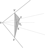
Figure 16: The fan $\Xi_{\Delta}$ drawn for $\Delta=\Delta(F_{2})$. It lies in a one dimension higher space $N^{\prime}_{\hbox{IR}}$ than $\Delta$, and is defined as the set of points hit by rays from the origin $\{0\}\in N^{\prime}_{\hbox{IR}}$ through $\bar{\Delta}$, where $\bar{\Delta}$ is the convex hull of the points $\bar{\nu}^{(i)}=(1,\nu^{(i)})$, which lie on a hyperplane of distance $1$ from the origin in $N^{\prime}_{\hbox{IR}}$. $\Xi_{\Delta}$ inherits its subdivison in a fan from the triangulation of $\Delta$. In this setting $\Delta$ is often called the trace of $\Xi_{\Delta}$.

8.3 Seiberg-Witten curves from the local B-model

We use now the construction of [180] to assign a local mirror description to the local $A$ model geometry. This construction assigns new variables $y_{i}$ $i=1,\ldots r$ to every field in the gauged $\sigma$-model, which are subject to relations defined from the $U(1)^{k}$ charge vectors $l^{(i)}$ $i=1,\ldots,k$ as

$$\prod_{l^{(i)}_{n}>0}y_{n}^{l^{(i)}_{n}}=\prod_{l^{(i)}_{n}<0}y_{n}^{-l^{(i)}_{n}}\$$ (8.4)

where we left open the dimension for the moment. The mirror manifold $\hat{\Xi}$ is given by the $r-k-1$ dimensional manifold [180]

$$P=\sum_{i=1}^{r}a_{i}y_{i}(t_{i})=0\ ,$$ (8.5)

where we solved the relations (8.4) in terms of $r-k$ variables $s_{i}$ which we will projectivize. This defines an $r-k-2$-dimensional manifold, which encodes the local geometry of the $A$ model and turns out to be in the limit discussed in the previous section the Seiberg-Witten curve of the associated field-theory! In addition to the curve we have to provide a meromorphic differential $\Lambda$ whose periods fulfill the Picard-Fuchs equations, which is associated to the quantum-cohomology of the $A$-model. These are derived from the charge vectors as in (7.5) and are identically fulfilled by any period over the form

$$\Lambda=-{\rm res}\left(\log(P){ds_{1}\over s_{1}}\wedge\ldots\wedge{ds_{r-k-2}\over s_{r-k-2}}\right)\ .$$ (8.6)

In order to convert (7.5) into a differential equation involving only on the invariant parameters $z_{i}=(-1)^{l^{(i)}_{0}}\prod_{n}a_{n}^{l^{(i)}_{k}}$ we must show that $\int_{C}\Lambda$ depends only on the $z_{i}$. This is essentially the case, in fact it is easy to see that $\int_{C}\Lambda$ transforms at worst by a constant shift under the projective $\,\hbox{IC}^{*}$ action on the $s_{i}$ as well as under the $k$ $\,\hbox{IC}^{*}$-star actions on the $a_{i}$ defined by the $l^{(i)}$. That is consistent with the fact that the differential equation has the constant as solutions, as has to be expected for the Picard-Fuchs equation for a meromorphic differential with non-vanishing residue.

Let us convert $\Lambda$ for the relevant case $r-k=3$ into a differential in a patch of the projective coordinates $s_{1},s_{2},s_{3}$. As usually $C$ is a cycle on the $1$-complex dimensional manifold and and $\gamma$ is a cycle around $P=0$ enforcing the residue

$$\begin{array}[]{rl}&-\displaystyle{\int_{C}\int_{\gamma}{\rm log}(P){{\rm d}s_{1}\over s_{1}}\wedge{{\rm d}s_{2}\over s_{2}}=-\int_{C}\int_{\gamma}{\rm log}(P){\rm d}{\rm log}(s_{1})\wedge{{\rm d}s_{2}\over s_{2}}}=\\[8.53581pt] &\displaystyle{\int_{C}\int_{\gamma}{\rm log}(s_{1}){{\rm d}P\over P}\wedge{{\rm d}s_{2}\over s_{2}}=\int_{C}{\rm log}(s_{1}){{\rm d}s_{2}\over s_{2}}}=:\int_{C}\lambda\ .\end{array}$$ (8.7)

For $F_{2}$ the relations (8.4) are $y_{1}y_{2}=y_{3}^{2}$ and $y_{3}y_{4}=y_{0}^{2}$ and will be identically solved by identifying $(y_{0};y_{1},y_{2},y_{3},y_{4})=(st;sz,s/z,s,st^{2})$. Projectivizing $s=1$ gives

$$P=a_{1}z+a_{2}{1\over z}+a_{3}+a_{0}t+a_{4}t^{2}=0\ ,$$ (8.8)

which depends de facto only on the good coordinates $z_{S}:=z_{1}={a_{1}a_{2}\over a_{3}^{2}}$ and $z_{F}:=z_{2}={a_{3}a_{4}\over a_{0}^{2}}$ and we might use the $(\,\hbox{IC}^{*})^{2}$-action to set $a_{1}=a_{4}=1$ and in the following. The differential $\Lambda$ becomes by (8.7)

$$\lambda={\rm log}(t){{\rm d}z\over z}\ .$$ (8.9)

What remains at this point is to implement the double scaling limit discussed in (7.21), i.e. $z_{S}\sim\epsilon^{4}\Lambda^{4}$, $t_{W^{\pm}}=t_{2}\sim\epsilon a$. The corresponding scaling can be achieved by setting $a_{3}=\epsilon^{-2}$ and $a_{2}=\Lambda^{4}$. Netxt we bring (8.8) in the standard form (4.39); in order to get rid of the next to leading term in $t$ we define

$$t=:(\sqrt{2}x-{a_{0}\over 2})$$ (8.10)

that converts (8.8) into

$$P=z+{\Lambda^{4}\over z}+2\,(x^{2}-u)=0$$ (8.11)

with $u:=-{1\over 2}\left(a_{3}-{a_{0}^{2}\over 4}\right)$. As $u$ is required to be finite we must identify $2\epsilon^{2}u:=-\left(1-{1\over 4z_{2}}\right)$, which gives precisely the definition of the Seiberg-Witten curve in the physical limit ! Inserting (8.10) into (8.9) shows that the leading pieces of the periods can go with

$$\int{\rm log}(x-{\cal O}(\epsilon)){{\rm d}z\over z}=-\log({\cal O}(\epsilon))\int{{\rm d}z\over z}+\epsilon\int x{{\rm d}z\over z}\ .$$

In fact the residue around the first term reproduces periods which go with $(1\ {\rm or}\ S)+\ldots$ and the residue around the second term reproduces periods, which go with $\sqrt{\alpha^{\prime}}(a\ {\rm or}\ a_{D})$ in agreement with (7.25).

8.4 Including matter

The inclusion of matter on the type IIa side is very simple. Basically we have to introduce in the ruled surface over the $\hbox{IP}^{1}$ a singular fiber which splits into two $\hbox{IP}^{1}$s as indicated in figure Fig.15. This is the situation explained more generally in [211]. Similar as in (7.3) one may start the consideration in six dimensions with a configuration of vanishing cycles, which give rise to a gauge group $G$ of rank $r+1$ with a vector, a complex scalar and two fermions, all in the adjoint. Let us consider a decomposition of $G$ into $H\times U(1)\subset G$. After fibering that configuration, the position on the base can be viewed in the right geometric setting as the scalar vev in the $U(1)$ direction of the Cartan subalgebra of $G$, which breakes the group generically to $H$ except at the point where the scalar vev is zero. That leaves generically a gauge group $H$ with matter from the decomposition of the complex scalar (and the fermionic completion) into $H\times U(1)$. Here we have simply $SU(2)\times U(1)\subset SU(3)$ and expect one matter hypermultiplet in the fundamental representation.

The toric description of the situation is depicted in Fig.15 and the toric data are

$$\begin{array}[]{rrrrrrr}K&F&F-E&E&S&S^{\prime}&\cr D_{0}&D_{1}&D_{2}&D_{3}&D_{4}&D_{5}&\cr\left(\matrix{0\cr 0}\right)&\left(\matrix{-2\cr-1}\right)&\left(\matrix{0\cr 1}\right)&\left(\matrix{1\cr 1}\right)&\left(\matrix{-1\cr 0}\right)&\left(\matrix{1\cr 0}\right)&\end{array}$$

The corresponding charges of the $U(1)^{3}$ gauged Landau-Ginzburg model can be obtained from the calculation of the Mori-vectors

$$\begin{array}[]{rrl}B:&l^{(1)}&=(\phantom{-}0;\phantom{-}1,\phantom{-}1,\phantom{-}0,-2,\phantom{-}0)\cr F-E:&l^{(2)}&=(-1;\phantom{-}0,-1,\phantom{-}1,\phantom{-}1,\phantom{-}0)\cr E:&l^{(3)}&=(-1;\phantom{-}0,\phantom{-}1,-1,\phantom{-}0,\phantom{-}1)\cr\end{array}$$ (8.12)

The relations (8.4) are fulfilled by introducing $(st,zs,s/z,t/z,s,t^{2})$ which leads after projectivisation to the constraint

$$P=a_{1}z+a_{2}{1\over z}+a_{3}{t\over z}+a_{4}+a_{0}t+a_{5}t^{2}=0\ .$$

Replacing again $t\rightarrow\sqrt{2}x-{1\over 2}a_{0}$ and substituting $z\rightarrow y-(x^{2}-u)$ we convert that precisely into the form (4.23)

$$y^{2}=(x^{2}-u)^{2}-\Lambda^{3}(x+m)$$

with the parameters

$$u=-{1\over 2}(a_{4}-{1\over 4}a_{0}^{2}),\quad\Lambda^{3}=\sqrt{2}a_{3},\quad\Lambda^{3}m=(a_{2}-{1\over 2}a_{3}a_{0})\ ,$$ (8.13)

In particular from (7.19) with (3.2) $\kappa=3$ we know that $z_{B}\sim\epsilon^{3}\Lambda^{3}$ and hence $((4z_{E}z_{F-E})^{-1}-1)\sim 2\epsilon u^{2}$ and $(z_{E}-{1\over 2})\sim\Lambda^{3}m\epsilon$, which is perfectly consistent with the picture of growing base, a mass generation of the gauge boson from wrapping the $D$-2-brane around the non-isolated curve and a mass generation of the hypermultiplet from wrapping the isolated curve.

8.5 Other Gauge groups

The toric diagrams for the generalizations to $A_{n}$ groups are shown in Fig.17. Using this toric representation it is simple to calculate, using the the description given in appendix E, the following intersections

$$FC_{i}C_{j}=\cases{-2&if $i=j$\cr\phantom{-}1&if $|i-j|=1$\cr\phantom{-}0&otherwise}\ .$$ (8.14)

For $A_{n}$ more matter in the fundamental representation can be easily added by further blowing up the same toric diagram compare [207].

By exactly same construction as above, this reproduces the Seiberg-Witten curves, with more matter in the fundamental representation.

Figure 17: In the left part of the picture we show the trace of a three dimensional fan $\Xi_{\Delta}$ with apex at the origin with the hyperplane $H$ at distance one from the origin, see figure 15 for the definition of the trace. This toric diagram corresponds to a configuration of ruled surfaces over $\hbox{IP}^{1}$ indicated on the left. If all components $C_{i}$ shrink simultaneously (or partly) we get Gorenstein singularities in the non-compact Calabi-Yau and pure $A_{n}$ (or a subgroup) as gauge theory. The right part shows the modification by a $\hbox{IP}^{1}$ blow up, which leads to one matter multiplet in the fundamental representation.

$\bullet$ Field theory from worldsheet instantons: Let us finally comment on the detailed field theoretic interpretation, which this picture assigns to certain worldsheet instantons. We consider the pure $SU(2)$ case and denote by $N_{n,m}$ the instanton number of a worldsheet instanton, which wraps $m$-times around the base and $n$-times around the fiber of the Hirzebruch surface $F_{n}$. The Kählermoduli of the fiber and the base are $t_{W}^{\pm}$ and $t_{S}$ respectively.

We find $N_{0,1}=-2$, $N_{0,i}=0$, $\forall i>1$. What is the field theoretic interpretation of this worldsheet instanton contribution ? Using (7.21) and (6.53) we can express the gauge coupling as

$$-i\tau={4\pi\over g^{2}}+{\theta\over 2\pi i}=\partial_{t_{W}^{\pm}}^{2}{\cal F}=\sum_{n=0}^{\infty}\sum_{m=1\atop k=1}^{\infty}N_{n,m}m^{2}{q_{S}^{nk}q_{W^{\pm}}^{mk}\over k}.$$

In the perturbative limit we have to consider only the contributions with $n=0$ and can sum over $k$ to obtain $\partial_{t_{W}^{\pm}}^{2}{\cal F}_{pert}=-2\sum_{k=1}^{\infty}{q_{W^{\pm}}^{k}\over k}=2\,\log(1-q_{W^{\pm}})$. In the limit (7.21) $q_{W^{\pm}}\sim 1-\epsilon a$ and so $-i\tau_{pert}=2\log(a)+const.+{\cal O}(\epsilon)$. In other words the instanton, which wraps only the base produces exactly the one-loop contribution of the field theory. It is easy to see that one gets the general perturbative one-loop part (4.36) if one replaces the $\hbox{IP}^{1}$ by a $ADE$ Hirzebruch-Jung sphere three.

More generally it was observed in [10] that the spacetime instantons ${\cal F}_{n}$ in the expansion (3.12), which are made explicit in the table above (3.44), describe nothing else then the growth of the worldsheet instantons. More precisely if we parameterize the growth by $N_{n,m}=\gamma_{n}m^{4n-3}$ then ${\cal F}_{n}={2^{3(3n-1)}\over(4n-3)!}\gamma_{n}$.

Appendix A BPS multiplets

Let us briefly remind the reader about a basic fact from the representation theory of extended supersymmetry algebras [88]. If $N>1$ the general supersymmetry algebra

$$\begin{array}[]{rl}\{Q^{I}_{\alpha},Q_{\dot{\beta}\,J}\}&=2\sigma^{\mu}_{\alpha\beta}P_{\mu}\delta^{I}_{J}\\ \{Q^{I}_{\alpha},Q^{J}_{\beta}\}&=2\sqrt{2}\varepsilon_{\alpha\beta}Z^{IJ}\\ \{Q_{\dot{\alpha}I},Q_{\dot{\beta}J}\}&=2\sqrt{2}\varepsilon_{\dot{\alpha}\dot{\beta}}Z^{*}_{IJ}\end{array}$$ (A.1)

allows in general for a nonvanishing central extension $Z^{IJ}$, $I,J=1,\ldots,N$, which is antisymmetric in $IJ$. For $N$ even one can skew-diagonalize $Z=\varepsilon\otimes{\rm diag}(Z_{1},\ldots Z_{N\over 2})$ by a basis transformation. Defining new generators ${}^{k}\delta_{\alpha}^{\pm}$, $k=1,\ldots,{N\over 2}$

$${{}^{k}}\delta^{\pm}_{\alpha}={1\over 2}\left(Q^{2k-1}_{\alpha}\pm\varepsilon_{\alpha\beta}{(Q^{2k}_{\beta})}^{{\dagger}}\right)$$ (A.2)

we can write the supersymmetry algebra in the restframe ($P_{0}=M$) in the form

$$\{{{{}^{k}}\delta^{\pm}_{\alpha},({{}^{k}}\delta_{\beta}^{\pm})}^{{\dagger}}\}=\delta_{\alpha\beta}(M\pm\sqrt{2}Z_{k})\ ,$$ (A.3)

where all other anticommutators vanish. As the physical Hilbert space norm must be positive definit ${\langle}\phi|\{\ldots\}|\phi{\rangle}\geq 0$ one has $M\geq\sqrt{2}|Z_{k}|$. If none of these inequalities is saturated one gets $2^{2N}$ states, which can be built by application of the creation and annihilation operators on a “vacuum” state, which allows for a representation with highest possible spin difference. Those representations are called ‘long’. If $r$ of these inequalities are saturated one gets in the same way only $2^{2N-r}$ states and the corresponding representations are called short, ultrashort etc. In particular for $N=2$ the short multiplet is the BPS-multiplet and, as mentioned, those states can be viewed as topological subsector of the theory.

Appendix B Some properties of the fundamental region of discrete subgroups in ${\rm PSL}(2,\hbox{IR})$

The upper half plane IH is parameterized by $\tau=x+iy$ with $x\in\hbox{IR}$, $y\in\hbox{IR}_{0}^{+}$. ${\rm PSL}(2,\hbox{IR})$ acts on IH by $\tau\mapsto{A\tau+B\over C\tau+D}$ with $M=\left(\matrix{A&B\cr C&D}\right)\in{\rm SL}(2,\hbox{IR})$, i.e. $A,B,C,D\in\hbox{IR}$ and $AD-BC=1$. As explained e.g. in [41] [42] the fundamental region $F$ in IH of a discrete subgroup $\Gamma\subset{\sl SL}(2,\hbox{IR})$ will be a polygon bounded arcs (including the ones of infinite radius), which are perpendicular to the real axis $E$. The reader will check that (2.4) maps indeed the interior of these arcs to the exterior. All monodromy matrices (3.27) and (3.29) have $|{\rm Tr}(M)|=2$, such elements of ${\rm SL}(2,\hbox{IR})$ are known as parabolic elements and conjugated to shifts. The significance of ${\rm Tr}(M)^{2}-4$ is that it is the discriminant of the fixpoint equation $C\tau^{2}+(D-A)\tau-B=0$ of the ${\rm PLS}(2,\hbox{IR})$ action. So if $C\neq 0$ the fixpoint of a parabolic element is on $E$. If $C=0$ the parabolic element is a shift $\tau\mapsto\tau+m$ with fixpoint $\tau=i\infty$. If $|{\rm Tr}(M)|<2$ ($|{\rm Tr}(M)|>2$) the element is called elliptic (hyperbolic). An elliptic element $M$ for which $\rho$, as in $\rho+\rho^{-1}={\rm Tr}(M)^{2}-2$, is an n’th root of unity corresponds to a transformation of order $n$ ($M^{n}=\pm 1$) in ${\rm PSL}(2,\hbox{IR})$. For parabolic elements one defines formally $n=\infty$. It is easy to check that in ${\rm PSL}(2,\hbox{ZZ})$ one has only $n=2,3$ or $\infty$. The arcs bounding $F$ contain fixed points $P_{\gamma}$ of elliptic or parabolic elements in $\Gamma$ and the sum of the inner angles at the equivalent fixed points on the boundary of $F$ is $2\pi/n$. This is clear from the fact that $n$ equivalent regions will meet at the fixpoint of order $n$ and since (2.4) is angle preserving each of these regions occupy the same angle at $P_{\gamma}$. In hyperbolic geometry the metric is ${\rm d}s={|{\rm d}\tau|\over y}$ and the area differential ${\rm d}^{2}\sigma={{\rm d}x{\rm d}y\over y^{2}}$. The ${\rm PSL}(2,\hbox{IR})$ action on IH obviously preserves distances and areas in hyperbolic geometry. The sides of in the boundary of the fundamental region are pairwise identified and the area of the normal polygons with $2n$ sides is easily calculated to be

$$A=2\pi(n-1-\sum_{fp}{1\over n_{i}})\ .$$ (B.1)

E.g.the standard fundamental region of ${\rm SL}(2,\hbox{ZZ})$, whose boundary contains the parabolic fixpoint of $T$: $i\infty$ the $Z_{2}$ fixpoint of $S$: $i$ and the cycle of $Z_{3}$ fixpoints: of $(TS)$: $\exp{2\pi i\over 6}$ and of $(ST)$: $\exp{2\pi i\over 3}$ is $A_{0}=2\pi(2-1-1/3-1/2)={\pi\over 3}$. For subgroups $\Gamma$ of ${\rm SL}(2,\hbox{ZZ})$ the area will clearly be a multiple $\mu$ of the the area $A_{0}$, which is known as the index of $\Gamma$. Subgroups of small index are classified [39].

Isometric circles  of an element $M\in\Gamma$ are defined by $|Cz+D|^{2}=1$. Their radius is $1/|C|$ and their center is at $({\rm Im}(\tau)=0,{\rm Re}(\tau)=CD/|C|^{2})$. If $\Gamma$ has a translation $\tau\rightarrow\tau+b$ the construction of the fundamental region is especially simple. One draws a vertical strip of width $b$ called $R_{\infty}$. The fundamental region is the union of $R_{\infty}$ with the exterior of every isometric cycle. As we have only parabolic elements to our disposal in our application the isometric cycles have to fit exactly in the strip $R_{\infty}$ as in Fig.4.

Appendix C Weighted projective form of the $\Gamma_{0}(2)$ curve, Picard-Fuchs equations and discriminants

The elliptic curve ${\cal E}$ which gives rise to $\Gamma(2)$ or to $\Gamma_{0}(2)$ can be represented in different forms. We will first chose a representation, which will prove useful later when we discuss CY manifolds and describe it by the zero locus of the quasi-homogeneous degree $k=4$ polynomial

$$p={a_{1}x_{1}^{4}}+{a_{2}x_{2}^{4}}+{a_{3}x_{3}^{2}}-{a_{0}}x_{1}x_{2}x_{3}\ .$$ (C.1)

in the weighted projective space $\hbox{IP}^{2}(1,1,2)$. See section 5.2 for the definitions. Clearly this manifold is one complex dimensional and from (5.17) with $k=4$, $w_{1}=w_{2}=1$ and $w_{3}=2$ it has vanishing first Chern class $c_{1}=0$, hence it is a torus.

$\bullet$ Picard-Fuchs equations from scaling symmetries. The parameterization in (C.1) is redundant as an elliptic curve will have only one independent parameter in the defining polynomial, which deforms the complex structure. In fact we have three $\,\hbox{IC}^{*}=(\,\hbox{IC}\setminus\{0\})$ actions on the parameters as $a_{i}\mapsto\lambda^{k/w_{i}}a_{i}$, $x_{i}\mapsto\lambda^{-1}x_{i}$ and $a_{0}\mapsto\lambda a_{0}$ for $i=1,2,3$ leave (C.1) invariant. We might therefore introduce later $z={a_{1}a_{2}a_{3}^{2}\over a_{0}^{4}}$ as invariant parameter. The period integral can be defined by the residue expression

$$\tilde{\varpi}_{i}=\oint_{C_{i}}{1\over 2\pi i}\oint_{\Gamma_{\epsilon}}{a_{0}{\rm d}\mu\over p}\ .$$ (C.2)

Here ${\rm d}\mu=\sum_{i=1}^{3}(-1)^{j}w_{i}x_{i}{\rm d}x_{1}\ldots\widehat{{\rm d}x_{i}}\ldots{\rm d}x_{3}$ and the hat means omission. $\Gamma_{\epsilon}$ is a small circle looping around $p=0$ and $C_{i}\in H^{1}({\cal E},\hbox{ZZ})$ is an element in the integral homology of ${\cal E}$.

Note that in $\tilde{\varpi}$ we put an $a_{0}$, which is essential to keep the $(\,\hbox{IC}^{*})^{3}$ invariance, which we will use now to derive the Picard-Fuchs equation. After the derivation we will use the more conventional form of period integral $\varpi={1\over a_{0}}\tilde{\varpi}$ . First note, using $\vartheta_{i}:=a_{i}\partial_{a_{i}}$, $[a_{i},\vartheta_{i}]=-a_{i}$, $\theta_{z}:=z\partial_{z}$ and $\vartheta_{i}f(z:=\prod_{k=1}^{n}a_{k}^{l_{k}})=l_{i}\theta_{z}f(z)$ the following identities

$$\begin{array}[]{rl}0=&a_{1}a_{2}a_{3}^{2}a_{0}(\partial_{1}\partial_{2}\partial_{3}^{2}-\partial_{0}^{4}){{\rm d}\mu\over p}\\[5.69054pt] =&a_{0}\left(\vartheta_{1}\vartheta_{2}\vartheta_{3}(\vartheta_{3}-1)-z\prod_{i=0}^{3}(\vartheta_{0}-i)\right){{\rm d}\mu\over p}\\[5.69054pt] =&\left(\vartheta_{1}\vartheta_{2}\vartheta_{3}(\vartheta_{3}-1)-z\prod_{i=1}^{4}(\vartheta_{0}-i)\right){a_{0}{\rm d}\mu\over p}\\[5.69054pt] =&(2\theta_{z}^{3}(2\theta_{z}+1)-z\prod_{i=1}^{4}(4\theta_{z}-i)){a_{0}{\rm d}\mu\over p}\\[5.69054pt] =&\theta_{z}(4\theta_{z}-2)[\theta_{z}^{2}-z(4\theta_{z}+1)(4\theta_{z}+3)]{a_{0}{\rm d}\mu\over p}\\[5.69054pt] =&\theta_{z}(4\theta_{z}-2){\tilde{\cal L}}{a_{0}{\rm d}\mu\over p}\end{array}$$

From the last expression it is clear that $\theta_{z}(4\theta_{z}-2){\cal L}\tilde{\varpi}=0$. From the four solutions to this equation only the two which fulfill ${\tilde{\cal L}}\tilde{\varpi}=0$ have the right asymptotic at $z=0$ to be periods of ${\cal E}$. It is straightforward to see that this system after the variable substitution $z=(64u^{2})^{-1}$ is equivalent to ${\cal L}\varpi=0$ with ${\cal L}$ as in (3.40).

The fact that two elliptic curves have the same Picard-Fuchs equation does not quite imply that they belong to the same parameterization family, which has a unique $\Gamma\in SL(2,\hbox{ZZ})$ and a unique $\tau(u)$. The ratios of the period integrals over the generating elements of $H^{1}({\cal E},\hbox{ZZ})$ have also to agree. This is for example not the case for curves, which are only isogeneous, here $\tau(u)$ differs by an integer factor.

We can complete the check that (C.1) is a $\Gamma(2)$ curve by calculating the $j$-invariant. We may use first an invariance transformation of the $\hbox{IP}^{2}(1,1,2)$ $x_{1}\mapsto\sqrt{i}x_{1}$, $x_{2}\mapsto\sqrt{i}x_{2}$ and $x_{3}\mapsto x_{2}+\sqrt{2u}x_{1}x_{2}$ and go to inhomogeneous coordinates $x_{2}=1$, $x_{1}=x$, $x_{3}=y$ so that the constraint $p=0$ looks like

$$y^{2}\equiv x^{4}+2ux^{2}+1\ .$$ (C.3)

This is further transformed to the Weierstrass form (4.13) (comp. footnote 25) with $3g_{2}=3+u^{2}$ and $27g_{3}=9u(1-u^{3})$ so the $j$-invariant is

$$j={(3+u^{2})^{3}\over 27(1-u^{2})^{2}}.$$ (C.4)

Comparing that with (4.17) solves the inversion problem for the triangle functions and by comparing it with the asymptotic of $\tau(u)$ (C.3) is established as $\Gamma(2)$ curve. From (C.4) we also see that $u$ branches sixfold over $j$, which is another way to see that $\Gamma(2)$ is of index six in $SL(2,\hbox{ZZ})$. If we do not introduce the double covering variable $u$ but just rescale $z=64\tilde{z}$, then we get $\Gamma_{0}(2)$ of index $3$ and the hypergeometric system (3.37) with (note that we exchanged $0$ and $\infty$) $\alpha_{\infty}=1/2$, $\alpha_{0}=0$ and $\alpha_{1}=0$, i.e the system $(1/4,3/4,1)$.

In (C.2) with $a_{0}=1$ we might use (C.3) and perform the integration over the loop $\Gamma_{\epsilon}$ in the $y$-plane. This leads to the integral

$$\varpi_{i}=\oint_{C_{i}}{{\rm d}x\over{{\rm d}p\over{\rm d}y}|_{p=0}}=\oint_{C_{i}}\omega\ .$$ (C.5)

with the holomorphic $(1,0)$-form $\omega={{\rm d}x\over y}$ as derived in sec 4.2.1.

$\bullet$ Discriminant and Picard-Fuchs equation for general Hyperelliptic curves:

The residue expression (C.2) is well defined under the equivalence relation in $\hbox{IP}^{n}(\vec{w})$ only for $c_{1}=0$ manifolds (5.17). The above symmetry considerations are a powerful tool and often sufficient to derive the Picard-Fuchs equations for $K3$ and higher dimensional CY, see [140], [141] and references therein for additional techniques. For higher genus Riemann surfaces $c_{1}<0$ and we will need a little more algebra to derive the Picard-Fuchs equations. Let

$$\begin{array}[]{rl}f&=a_{0}x^{m}+a_{1}x^{m-1}+\ldots+a_{m}\\[5.69054pt] g&=b_{0}x^{n}+b_{1}x^{n-1}+\ldots+b_{n}\\[5.69054pt] \end{array}$$ (C.6)

polynomials of degree $n$ and $m$. The resultant $R(f,g)$ is defined as the determinant $|M|$ of the $(n+m)\times(n+m)$ matrix see e.g. [200]

$$\matrix{n\!\!\!&\left\{\phantom{\matrix{a_{1}\cr a_{2}\cr a_{3}\cr a_{4}}}\right.\cr m\!\!\!&\left\{\phantom{\matrix{a_{1}\cr a_{2}\cr a_{3}\cr a_{4}}}\right.}\!\!\!\!\!\!\!\!\!\!\!\left|\matrix{a_{0}&a_{1}&\ldots&a_{m}&0&&\ldots&0\cr 0&a_{0}&\ldots&a_{m-1}&a_{m}&0&\ldots&0\cr&&&\ldots&&&&\cr&0&\ldots&0&a_{0}&a_{1}&\ldots&a_{m}\cr b_{0}&b_{1}&\ldots&b_{n}&0&&\ldots&0\cr 0&b_{0}&\ldots&b_{m-1}&b_{n}&0&\ldots&0\cr&&&\ldots&&&&\cr&0&\ldots&0&b_{0}&b_{1}&\ldots&b_{n}}\right|$$ (C.7)

It is clear that this determinant vanishes only if $f,g$ have a common root or $a_{0}=b_{0}=0$. Now define $\vec{m}=(x^{m-1},\ldots,1)^{t}$ and $\vec{n}=(x^{n-1},\ldots,1)^{t}$. Obviously $(f\cdot\vec{m},g\cdot\vec{n})^{t}=M\cdot(\vec{m},\vec{n})^{t}$. Cramers rule applied to the last entry $1$ in $(\vec{m},\vec{n})^{t}$ gives $R(f,g)=|M|=|M_{n+m}|$, which implies that $R(f,g)=a(x)f(x)+b(x)g(x)$ where $a(x)$ ($b(x)$) is of degree $n-1$ ($m-1$).

This is useful for the derivation of the Picard-Fuchs equation for the period $\varpi=\oint\omega$ of the hyperelliptic Riemann surface $y^{2}=p(x,u_{i})$ with holomorphic differential $\omega={{\rm d}x\over y}$. The discriminant is given by the resultant of $p=0$ and $p^{\prime}:={{\rm d}\over{\rm d}x}p=0$ i.e. $\Delta(u_{i})=R(p,p^{\prime})$. As we just shown $\Delta=ap+bp^{\prime}$. We want find differential relations of the form ${\cal L}(u_{i}){{\rm d}x\over y}={\partial h\over\partial x}{\rm d}x$. Derivatives on $\omega$ w.r.t. the moduli $u_{i}$ produce ${\phi(x,u_{i}){\rm d}x\over y^{n}}$ and we have to relate this terms up to exact terms to ${{\rm d}x\over y}$. To reduce the degree of $y$ in the denominator one uses the following algorithm. By partial integration we have up to exact terms

$${\phi(x)\over y^{n}}={1\over\Delta}{a\phi+{2\over n-2}(b\phi)^{\prime}\over y^{n-2}}.$$

This substitution increases the powers of $x$ in the numerator. They have to be lowered by expressing the highest power in $x$ in terms of lower ones in terms of $p$ or $p^{\prime}$ and lower powers. In the later case a partial integration must follow. Combining these steps the desired relations ${\cal L}(u_{i})\varpi=0$ can be derived.

For the calculation of the discriminante of the weighted projective Calabi-Yau hypersurfaces it is certainly not a practical way to use the generical alogarithm (C.7) iteratively on $p=0$ and ${{\rm d}\over{\rm d}x_{i}}p=0$. Direct elimination of the coordinates $x_{i}$ using the symmetries leads much quicker to the result, whose complexity grows however rapidly with the number of moduli. Note also that to find all possible components of the discriminate one has to test $p=0$ and ${{\rm d}\over{\rm d}x_{i}}p=0$ on all strata, i.e. for all allowed combinations of $x_{i_{1}}=\ldots x_{i_{k}}=0$. The component of the discriminante, which is calculated for all $x_{i}\neq 0$ is called principal part. For (7.4) it is $\Delta_{c}$, while for $x_{3}=x_{4}=x_{5}=0$ we get the independent component of the discriminante $\Delta_{s}$. For complete intersections examples see [141].

Appendix D Instantons corrected triple intersections for the practioner

In this appendix we want to summarize how to calculate the periods the mirror map and the triple intersections on general toric CY $d$-folds following largely [140] [141] [159] [161] and especially [162]. The solution for the periods is given by eq. (D.5) the mirror map is defined in (D.6) and (D.7,D.8) give the basic instanton corrected triple coupling. The reconstruction of the other ones, for $d>4$ a problem, is described in section (D.2). There are two conceptional straightforward but technically involved problems which must be solved before applying these formulas. The calculation of the classical intersection numbers, is described in appendix D, for the practical application there is a program [182]. The second is the construction of the Kähler cone respectively its dual the Mori-cone. It is described in [139] and a problem which arises in this context namely the triangulation of polyhedra can be solved with the program [183].

D.1 Frobenius algebras

To obtain all $k$-point functions we introduce some basic notions of Frobenius algebras. In this section, all vector spaces are finite dimensional. A Frobenius algebra is a commutative graded algebra $A=\oplus_{i=0}^{d}A_{(i)}$, generated by $A_{(1)}$, has $A_{(0)}={\bf C}\cdot 1$, and a nondegenerate degree $n$ bilinear symmetric invariant pairing ${\langle},{\rangle}:A\times A\rightarrow{\bf C}$. Note that because we require generation by $A_{(1)}$, this notion is slightly stronger than the usual notion of a Frobenius algebra. We give some well-known examples from geometry. Let ${\bf P}$ be a complete toric variety, and $A^{*}({\bf P})$ be its Chow ring. Then $A^{*}({\bf P})\otimes{\bf C}$ is a Frobenius algebra. The pairing here is the Poincaré pairing. If $X$ is a hypersurface in ${\bf P}$, then it can be shown that the ring

$$\tilde{A}^{*}(X):=Im(A^{*}({\bf P})\rightarrow A^{*}(X))=A^{*}({\bf P})/Ann([X])$$ (D.1)

tensored with ${\bf C}$ is a Frobenius algebra. More generally, if $A$ is a Frobenius algebra, and $x\in A_{(1)}$ is a nonzero element, then $\tilde{A}:=A/Ann(x)$ is a Frobenius algebra with the induced pairing ${\langle}a+Ann(x),b+Ann(x){\rangle}:={\langle}a,b\cdot x{\rangle}$ having degree $d-1$.

Let $V_{1},V_{2},V_{3}$ be vector spaces, and $C:V_{1}\otimes V_{2}\otimes V_{3}\rightarrow{\bf C}$ be a three-point function. It is call $V_{1}$-nondegenerate if that $C_{(a,b,c)}=0$ for all $b,c$ implies that $a=0$. Similar notion of $V_{i}$-nondegeneracy applies. We call the form nondegenerate if it is $V_{i}$-nondegenerate for all $i$. Now suppose $C$ is $V_{3}$-nondegenerate. Then we have the following invertibility property. Let $D:V_{3}^{*}\otimes V_{4}\rightarrow{\bf C}$ be any bilinear form. Then the knowledge of the 3-form $E_{(a,b,d)}:=C_{(a,b,c_{i})}D_{(\gamma^{i},d)}$ ($\{c_{i}\},\{\gamma^{i}\}$ being dual bases), allows us to determine $D$ completely. In fact, there exists (in general not unique) a 3-form $F$ such that $D_{(\gamma,d)}=F_{(\gamma,\alpha^{i},\beta^{j})}E_{(a_{i},b_{j},d)}$. This is just the statement that the $V_{3}$-nondegenerate three-point function $C$ defines an onto map $V_{1}\otimes V_{2}\rightarrow V_{3}^{*}$, hence choosing a section gives us a left inverse $F$ to this map.

We now return to a Frobenius algebra $A$. it determines a collection of three point functions $C^{(ijk)}:A_{(i)}\otimes A_{(j)}\otimes A_{(k)}\rightarrow{\bf C}$ with $i,j,k\geq 0,i+j+k=d$. These three-point functions are $A_{(i)}$-nondegenerate whenever either $j=1$ or $k=1$ because $A_{(1)}\cdot A_{(i)}=A_{(i+1)}$.

D.2 Reconstruction

Let $A=\oplus_{i=0}^{d}A_{(i)}$ be a graded space with $A_{(0)}={\bf C}$ and equipped with a degree $d$ nondegenerate symmetric bilinear form $\eta$. Suppose we are given three-point function: $C^{(ijk)}:A_{(i)}\otimes A_{(j)}\otimes A_{(k)}\rightarrow{\bf C}$, $i,j,k\geq 0$ with the following properties:

• (a) (Degree) $C^{(ijk)}=0$ unless $i+j+k=d$.

• (b) (Unit) $C^{(0ij)}_{(1,b,c)}=\eta^{(i)}_{b,c}$.

• (c) (Nondegeneracy) $C^{(1ij)}$ is nondegenerate in the second slot.

• (d) (Symmetry) For any permutation $\sigma$ of 3 letters, $C^{(ijk)}_{(a,b,c)}=C^{\sigma(ijk)}_{\sigma(a,b,c)}$.

• (e) (Associativity)

$$C^{(i,j,d-i-j)}_{(a,b,c_{p})}\eta_{(d-i-j)}^{pq}C^{(i+j,k,d-i-j-k)}_{(d_{q},e,f)}=C^{(i,k,d-i-k)}_{(a,e,c_{p}^{\prime})}\eta_{(d-i-k)}^{pq}C^{(i+k,j,d-i-j-k)}_{(d_{j}^{\prime},b,f)}$$ (D.2)

where the $c$ and the $d$ are bases of the appropriate spaces.

Then $A$ is a Frobenius algebra with the product

$$a\cdot b=C_{(a,b,c_{p})}\eta^{pq}d_{q}.$$ (D.3)

The rules above are known as fusion rules. One can also build a $k$-form by fusing together 2- and 3-forms. The associativity law says that there will often be many ways to build a given $k$-form. Similarly the 3-forms are not independent. We claim that the forms of type $(i,j,d-i-j)$ for $i,j>1$ are determined by the those of type $(1,r,d-r-1)$. To see this without loss of generality, we can assume $1<d-i-j\leq i,j$. Now by the associativity law above with $k=d-i-j-1$ and the invertibility property of $C^{(i+j,k,d-i-j-k)}=C^{(i+j,k,1)}$, it follows that $C^{(i,j,d-i-j)}$ are determined in terms of forms of type $(i,d-i-j-1,j+1)$ and $(i+k,j,1)$. By the symmetry property, $(i,d-i-j-1,j+1)$ is equivalent to $(i,j+1,d-i-j-1)$. Thus we have reduced the value of $d-i-j$ by 1. By induction, we see that all $(i,j,d-i-j)$ can be expressed in terms of those of type $(1,r,d-r-1)$. In terms of the algebra $A$ itself, an alternative way to state the result is that all the products $A_{(i)}\otimes A_{(j)}\rightarrow A_{(i+j)}$ is determined by those of the form $A_{(1)}\otimes A_{(r)}\rightarrow A_{(r+1)}$ because $A$ is generated by $A_{(1)}$ and that

$$(a_{1}\cdots a_{i})(a_{i+1}\cdots a_{i+j})=a_{1}(a_{2}\cdots a_{i+j}).$$ (D.4)

D.3 Application

Let $X$ be a CY $d$-fold, and let ${\cal A}$ be the corresponding Frobenius subalgebra of $\oplus_{p=0}^{d}H^{p}(X,\wedge^{p}T^{*})$. Suppose mirror symmetry holds: there is a mirror family $X^{*}$ whose B-model algebra coincides with the A-model algebra of $X$. We shall now compute the Frobenius subalgebra ${\cal B}$ of the B-model algebra corresponding to ${\cal A}$. From our general discussion of Frobenius algebras, it is enough to compute the three-point functions $C$ of types $(1,r,n-r-1)$ which come with ${\cal B}$. Once we have a period expansion in the topological base (6.49)these can be easily obtained using eqns (6.50,6.51, 6.52). To obtain the coefficients in (6.49) we will use the fact [140] that the universal structure of the solution of the Picard-Fuchs equation on $X^{*}$ at the large radius point mirrors the primitive part of the vertical cohomology of $X$ and the leading structure of logarithm enables us to associate this solutions with the expansion of the periods in a topological base. This leads to a direct generalization of the formulas of [141] to some correlation functions on $d$-folds.

More precisely there are $h^{r,r}_{prim}(X)$ solutions $0\leq r\leq d$ with leading degree $r$ in the $\log(z_{i})$, which have the form

$$\tilde{\Pi}^{(r)}_{k}=\sum_{\Pi}{{}^{0}C^{d-r,1\ldots 1}_{k,i_{1},\ldots,i_{r}}}\bigl{(}{1\over r!}l_{i_{1}}\ldots l_{i_{r}}S_{0}+{1\over(r-1)!}l_{i_{1}}\ldots l_{i_{r-1}}S_{i_{r}}+\ldots+S_{i_{1},\ldots,i_{r}}\bigr{)},$$ (D.5)

here we defined $l_{i}:=\log(z_{i})$ and the $S_{i_{1},\ldots i_{r}}$ are holomorphic series in the $z_{i}$, whose explicit form are given in section (D.4). $\Pi$ means permutation over distinct indices see below Eq. (7.7) for an example. The map to an specific element of the cohomology $H^{d-r,d-r}$ of $X$ can be made precise by noting that the ${}^{0}C^{d-r,1\ldots 1}_{k,i_{1},\ldots i_{r}}$ are given by the classical intersection of that specific element with the intersection of divisors $J_{i_{1}}\cdot\ldots\cdot J_{i_{r}}$. We discuss the primitive part of the (co)homology generated by $J_{1}\ldots J_{h^{1,1}}$ only and by Poincare duality, this data fix the element in $H^{d-r,d-r}$ completely.

As mentioned above the covariant derivative $\nabla_{a}$ in [159] becomes the ordinary derivative in the flat complexified Kähler structure coordinates $t_{k}$. The coordinate change from the natural complex structure coordinates $z_{a}$ to the $t_{k}$ variables is given by the mirror map

$$t_{k}={\tilde{\Pi}^{(1)}_{k}(z_{i})\over\tilde{\Pi}^{(0)}(z_{i})}=\log(z_{k})+{S_{k}\over S_{0}}\ .$$ (D.6)

If we substitute this coordinate transformation in the normalized periods $\Pi_{i}^{(r)}={\tilde{\Pi}_{i}^{(r)}\over\tilde{\Pi}^{(0)}}$ some simplifications occur as the first sub-leading terms in the $t_{i}$ cancel out:

$$\Pi^{(r)}_{k}=\sum_{\Pi}{{}^{0}C^{d-r,1\ldots 1}_{k,i_{1},\ldots,i_{r}}}\bigl{(}{1\over r!}t_{i_{1}}\ldots t_{i_{r}}+{1\over(r-2)!}t_{i_{1}}\ldots t_{i_{r-2}}\hat{S}_{i_{r-1}}\hat{S}_{i_{r}}+\ldots+\hat{S}_{i_{1},\ldots,i_{r}}\bigr{)}.$$ (D.7)

Now we notice from the monodromy around $z_{i}=0$ ($t_{i}\rightarrow t_{i}+1$) that the periods $\Pi_{k}^{(r)}$ correspond to a expansion of $\alpha^{(0)}=\Omega$ in terms of the topological basis $\gamma_{(r)}^{k}$ of (6.49) $\alpha^{(0)}=\sum_{k,r}\Pi^{(r)}_{k}{\gamma}_{(r)}^{k}$.

The coupling $C^{(1,1,d-2)}_{a,b,c}:H^{1,1}\times H^{1,1}\times H^{d-2,d-2}\rightarrow\,\hbox{IC}$ is especially simple to obtain. Applying (6.52) in the case $k=0$ we have $\partial_{t_{a}}\alpha^{(0)}=\alpha^{(1)}_{a}$. This determines $\alpha^{(1)}_{a}$, hence all its coefficients. Now using (6.50) for $k=1$, (6.49) for $k=1,d-2$, ‘and the fact that ${\langle}\gamma^{(k)}_{a},\gamma^{(l)}_{b}{\rangle}=0$ for $k+l>d$, we see that

$$C^{(1,1,d-2)}_{a,b,c}=\partial_{t_{a}}g^{(2)d}_{b}\eta^{(2)}_{dc}=\partial_{t_{b}}\partial_{t_{b}}\Pi^{(2)}_{c}\ ,$$ (D.8)

where the $g^{(2)}$ are the coefficients of the $\gamma^{(2)}$ in the $\alpha^{(1)}$. Note that the last equation follows from the fact that $\Pi^{(r)}_{a}$ is an expansion in the dual base $\gamma^{a}_{(r)}$ and that the associativity of the classical parts in (D.5) is manifest. Eqs. D.7 D.5 are direct generalizations of eqs. (4.9) and (4.18) to the $d$-fold case. For $H^{1,1}$ we have always a canonical choice of the basis say $J_{1}\ldots J_{h^{1,1}}$, as there is a canonical basis for the tangent space of the moduli space corresponding to elements $H^{d-1,1}(X^{*})$, which is mapped by the monomial divisor mirror map to $H^{1,1}(X)$ and (D.8) reduces for $d=3$ to the expressions given in [140]. For $d>3$ there is a priori no canonical choice for the basis of $H^{d-2,d-2}$. However toric geometry can be used as in [146] to show that the graded ring

$${\cal R}=\,\hbox{IC}[\theta_{1},\ldots,\theta_{h^{1,1}}]/{\cal J},$$ (D.9)

where ${\cal J}$ is the ideal generated by the leading $\theta$-terms of Picard-Fuchs equations, gives, by the identification $\theta_{i}\rightarrow J_{i}$, a presentation of the primitive part of $H^{*,*}$. Because of Poincare duality it is of course sufficient to pick a basis of half of $H^{*,*}$ and as mentioned above the choice of the basis in $H^{1,1}$ is canonical. It was shown in [140] [141] [146] that any element of $\cal R$ can be mapped to a solution (D.5) , i.e. the ${}^{0}C^{d-r,1\ldots 1}_{i_{1},\ldots,i_{r}}$ are determined by the principal part of the Picard-Fuchs equation. This can be viewed as a proof of mirror symmetry at the level of the classical intersections, which readily generalizes to $d$-folds.

Now proceed by induction. Suppose we know (the coefficients of) the $\alpha_{(i)}$ and the three-point functions of types $(1,i,n-i-1)$ for $i=0,1,..,k$. Then by the invertibility property of a three-point function of type $(1,k,n-k-1)$ in a Frobenius algebra, we can solve for the $\alpha_{(k+1)}$ using (6.52). Thus the $\alpha^{(k+1)}$ are determined. By (6.49), we can write $\partial_{t_{a}}\alpha^{(k+1)}_{b}=\partial_{t_{a}}g^{(k+2)d}_{b}\gamma^{(k+2)}_{d}+\cdots$ (which is now known), arguing as before using (6.50) with $k$ replaced by $k+1$, and using the inner product property of the $\gamma$, we find that $C^{(1,k+1,n-k-2)}_{abc}=\partial_{t_{a}}g^{(k+2)d}_{b}\eta^{(k+2,n-k-2)}_{dc}$. Thus the three-point functions of type $(1,k+1,n-k-2)$ is also determined. This shows that all three-point functions of type $(1,k,n-k-1)$ for $k=1,2,..,n-1$ can be expressed in terms of the coefficients of $\alpha_{(0)}$ alone.

D.4 Explicit expressions for periods in toric varieties

Following [140] [141] we can determine the holomorphic series $S_{i_{1},\ldots,i_{r}}$ from the generators of the Mori cone. Consider a CY $d$-fold defined as complete intersection with $p$ polynomial constraints in a toric variety of dimension $d+p$. The generators of the Mori cone will be of the form

$$l^{(i)}=(\hat{l}^{(i)}_{0},\ldots,\hat{l}^{(i)}_{p-1};l^{(i)}_{1},\ldots,l^{(i)}_{q}),$$

where $q=d+p+h^{d-1,1}$. The series $S_{i_{1},\ldots,i_{r}}$ are obtained by the Frobenius method from the coefficients of the holomorphic function $\omega(\vec{z},\vec{\rho})$

$$\begin{array}[]{rl}\omega(z,\vec{\rho})&=\displaystyle{\sum c(\vec{n},\vec{\rho})\prod_{j=1}^{h^{1,d-1}}z_{j}^{n_{j}+\rho_{j}}}\\[8.53581pt] c(\vec{n},\vec{\rho})&=\displaystyle{{\prod_{k=1}^{p}\Gamma(1-\sum_{i=1}^{h^{1,d-1}}\hat{l}^{(i)}_{k}(n_{i}+\rho_{i}))\over\prod_{k=1}^{q}\Gamma(1+\sum_{i=1}^{h^{1,d-1}}l^{(i)}_{k}(n_{i}+\rho_{i}))}}\\[11.38109pt] S_{i_{1},\ldots,i_{r}}&=\partial_{\rho_{i_{1}}}\ldots\partial_{\rho_{i_{r}}}\omega(\vec{z},\vec{\rho})|_{\vec{\rho}=\vec{0}}\end{array}$$

Notably with leading behavior $S_{0}=1+\ldots$, $S_{i}=z_{i}+\ldots$.

This gives the explicit expansion of $C^{(d-2,1,1)}_{A,b,c}=^{0}C^{(d-2,1,1)}_{A,b,c}+{\cal O}(q_{i})$, with $q_{i}=e^{t_{i}}$. The latter has a conjectured interpretation as being the counting function for invariants of maps from the two sphere into $X$.

Appendix E Toric geometry in a nutshell:

In this appendix we want to review some basic facts about toric geometry, which were used in lectures. Even a basic introduction into toric geometry would require much more space, so the following is merely intended to list these facts and to give a guide to the mathematical literature or sources phycists might find useful. From the mathematical reviews [142] [143] the book of Fulton might be easiest to read for physicists and an useful recent introduction in the subject motivated from physics can be found in [76].

For illustration we work with the $F_{2}$ example see Fig.15 and remind the reader for convenience of our identification of the toric divisors

$$\begin{array}[]{rrrrrr}K&F&F&S&S^{\prime}&\cr D_{0}&D_{1}&D_{2}&D_{3}&D_{4}&\cr\left(\matrix{0\cr 0}\right)&\left(\matrix{-2\cr-1}\right)&\left(\matrix{0\cr 1}\right)&\left(\matrix{-1\cr 0}\right)&\left(\matrix{1\cr 0}\right)\ ,\end{array}$$ (E.1)

where we dropped the tildes. To every toric divisor $D_{i}$ $i=1,\ldots,k$ we associate a point $\nu^{(i)}$ in a $n$ dimensional lattice $N\sim\hbox{ZZ}^{n}$ and a variable $x_{i}$, here $D_{1}\sim(-2,-1)$ etc. The convex hull of the points defines a $n$ dimensional polyhedron $\Delta$ in $N_{\hbox{IR}}\sim\hbox{IR}^{n}$ see Fig.15 and we call the origin $\nu^{(0)}=(\vec{0})$. An additional data is the choice of a triangulation into $n$ dimensional simplices. It defines the Stanley-Reisner ideal which is generated by the intersection of those $D_{i}=\{x_{i}=0\}$ whose associated points do not share a common simplex. The latter condition has to be tested for simplices of any dimension yielding sets of indices of points $\{J\}$, which are not on a common simplex and the full Stanley-Reisner ideal ${\cal SR}$ is generated by

$$\prod_{\{J\}}D_{j_{1}}\cap\ldots\cap D_{j_{|J|}},\ \forall J\ .$$ (E.2)

We consider the $x_{i}$ as variables parameterizing $\,\hbox{IC}^{k}$ and define the $k-s$ dimensional toric variety following [187] (see also [188]) as $\,\hbox{IC}^{k}\setminus{\cal SR}$ modulo the $s$ equivalence relations

$$(x_{1},\ldots x_{k})\sim(\lambda_{(i)}^{l^{(i)}_{1}}x_{1},\ldots,\lambda_{(i)}^{l^{(i)}_{k}}x_{k})$$ (E.3)

with $\lambda_{(i)}\in\,\hbox{IC}^{*}$ and the $l^{(i)}$ $i=1,\ldots,k$ are an integral basis for the linear relations $\sum_{i=1}^{k}\nu^{(i)}l_{i}^{(p)}=0$ between the points in $\Delta$.

This definition applies to smooth toric varities. If there are singularities a discrete torsion group acting on $x_{i}$ has also be divided out. E.g in the $\hbox{IP}(\vec{w})$ examples these are the $Z_{n}$ actions.

The tricky part is the definition of those generators $l^{(k)}$, called edges of the Mori-cone [139] [143], which is defined by the secondary cone of strictly convex piecewise linear function on the fan $\Xi_{\Delta}$ Fig.16. The Kähler cone is dual to the cone defined by the convex piecewise linear functions on $\Xi_{\Delta}$ modulo the smooth functions on $\Xi_{\Delta}$. Pragmatical procedures, how to determine the Mori-cone and the Kähler cone for toric varieties be found in [166] [140] [148] [146] [76] also [180] discusses the problem. Often the Kähler cone restricts simply to the Kählercone of the (CY) hypersurface in the toric variety, which may be the main object of interest. The discussion of the CY Kähler cone, when this is not the case can be found in [148] [149].

If the triangulation is a star triangulation, i.e. every $n$ dimensional simplex $s_{j}$ has the origin $\nu^{(0)}$ as vertex, then we can associate a fan $\Sigma(\Delta)$ to the polyhedron $\Delta$ by viewing the vertices $\nu^{(i_{j})}\neq\nu^{(0)}$ of the simplex $s_{j}$ as vectors spanning the edges of a cone $\sigma_{j}$ from $\nu^{(0)}$, which is defined as $\sigma_{j}=\{\sum_{i_{j}}r_{i_{j}}\nu^{(i_{j})}|r_{i_{j}}\in\hbox{IR}^{+}\}$. The fan $\Sigma(\Delta)=\cup_{i}\sigma_{i}$ is the collection of all cones $\sigma_{i}$ (and its faces) and it is easy to obtain from $\Sigma$ a representation of the manifold in terms of charts and transition functions [142] [143].

i) The manifold is compact if the fan $\Sigma$ is complete, i.e. it covers all of $N_{\hbox{IR}}$, while an incomplete fan describes an non-compact affine toric variety, see [143] for a proof of that statement. For more instructive examples, especially $\hbox{IP}^{2}$, whose polyhedron is the hull of $(1,0)$, $(0,1)$, $(-1,-1)$, see [76].

ii) If all cones are spanned with positive coefficients by a subset of an integral basis for the lattice $N$, the manifold is smooth, again [143] can be consulted for the proof.

iii) Consider the cone $\sigma$. If the lattice points on each edge, which are nearest to the origin, lie all in a hyperplane $H$, which is in distance one from the origin, i.e it exists a $m$ in the dual space $M_{\hbox{IR}}={\rm Hom}(N_{\hbox{IR}},\hbox{IR})$ to $N_{\hbox{IR}}$ such that $H=\{x\in N_{\hbox{IR}}|{\langle}x,m{\rangle}=1\}$, and there are no lattice points $x\in\sigma$ with $0<{\langle}m,x{\rangle}<1$, then the affine toric variety defined by $\sigma$ has only canonical Gorenstein singularities.

$\bullet$ The $\hbox{IP}^{2}(1,1,2)$ example: For instance, as we check most easily by comparing the definition of the toric variety (5.13) with (E.3), $\hbox{IP}^{2}(1,1,2)$ can be defined by the polyhedron, which is the convex hull of the the points $\nu^{(1)}=(-2,-1)$, $\nu^{(2)}=(0,1)$, $\nu^{(3)}=(1,0)$. It has simplices $s^{\prime}_{1}=\{\nu^{(0)},\nu^{(1)},\nu^{(2)}\}$, $s_{3}=\{\nu^{(0)},\nu^{(2)},\nu^{(4)}\}$, $s_{4}=\{\nu^{(0)},\nu^{(1)},\nu^{(4)}\}$. Condition ii is not fulfilled for the cone $\sigma^{\prime}_{1}$. There is a canonical Gorenstein $\hbox{ZZ}_{2}$-singularity in the chart associated to $\sigma^{\prime}_{1}$. The lattice $N$ modulo the lattice $N^{\prime}$, which is spanned by the edges of $\sigma_{1}^{\prime}$, defines the torsion group, which is the $\hbox{ZZ}_{2}$ in the case at hand. It acts on the normalbundle to the fixed locus of $(x_{1},x_{2},x_{3})\mapsto(\mu x_{1},\mu x_{2},\mu^{2}x_{3})$ $\mu^{2}=1$ i.e. $(x_{1}=0,x_{2}=0,x_{3}=1)$, by $(z_{1},z_{2})\mapsto(-z_{1},-z_{2})$. Generally the order of the discrete group is the volume of unit cell in $N^{\prime}$ divided by the unit cell of $N\cap\sigma$. Similarly if $r$ weights $w_{i_{1}}\ldots w_{i_{r}}$ of a $\hbox{IP}^{n}(\vec{w})$ have a common factor $n$ one gets a $n+1-r$ dimensional singular cone and $\hbox{ZZ}_{n}$ action on the normal bundel to the stratum $x_{i_{1}}=\ldots=x_{i_{r}}=0$. For fuller explanation of weighted projective spaces we refer to [215]. Generally singularities can be resolved by adding points and making a finer subdivision into cones, such that property ii holds for all of them. For $\hbox{IP}^{2}(1,1,2)$ we achieve that by adding the point $\nu^{(3)}\in\sigma^{\prime}_{1}$ and splitting $s^{\prime}_{1}$ into $s_{1}=\{\nu^{(0)},\nu^{(1)},\nu^{(3)}\}$, $s_{2}=\{\nu^{(0)},\nu^{(2)},\nu^{(3)}\}$, i.e. the non-singular resolution of $\hbox{IP}^{2}(1,1,2)$ is $F_{2}$.

What makes smooth toric varieties so easy to deal with is the fact that linear relations of the type $\sum_{i}{\langle}m,\nu^{(i)}{\rangle}D_{i}=0$ with $m\in M_{\hbox{IR}}$, which may be written in coordinates as

$$\sum_{i=1}^{k}\nu^{(k)}_{i}D_{k}=0\ ,$$ (E.4)

are homological relation between the divisors classes, e.g. for $F_{2}$: $D_{1}=D_{2}=F$ and $S^{\prime}=S+2F$. The Chern class of the toric variety is simply

$$c(T_{A})=\prod_{i=1}^{k}(1+D_{i})\ ,$$ (E.5)

the Chern classes $c_{i}(T_{A})$ are terms, which are homogeneous in the $D_{i}$. The evaluation of intersection defined in $c_{d}(T_{A})$ gives by Gauss-Bonnet theorem the Eulernumber $\chi(A)$ of $A$. On the other hand $\chi(A)$ can be expressed by the sum of all simplices of maximal dimension [143]

$$\chi(A)=\#{\rm d-simplices}\ ,$$ (E.6)

here 4. Eqs. (E.2,E.4,E.5, E.6) are strong enough to calculate by a, in general very involved but otherwise straigthforward, algebraic manipulation all intersections $D_{i_{1}}\cdots D_{i_{d}}$ and in particular using (E.5) one can calculate the evaluation of the Chern classes on the divisors.

Special hypersurfaces $X$ can be described in $A$ by combinations of toric divisors $L=\sum_{i}a_{i}D_{i}$. The first Chern class on the normal bundle is just

$$c_{1}({\cal N})=\sum_{i=1}^{k}a_{i}D_{i}$$ (E.7)

Refering back to section (5) we see by (5.14,5.15,5.16,E.5) that the choice $H=\sum_{i=1}^{k}D_{i}$ leads to $c_{1}(T_{X})=0$ for the singular variety defined by $H$. It was shown by Batyrev that the requirement of transversality of the constraint $H=0$ and the requirement that only canonical Gorenstein singularities appear on $H$, which is necessary to get $c_{1}(T_{X}^{smooth})=0$, leads to a combinatorial condition for the polyhedron $\Delta$ called reflexivity, by which a natural dual polyhedron $\Delta^{*}$ can be defined. Moreover the divisor $H^{*}=\sum_{i=1}^{k^{*}}D_{i}^{*}$ in the toric variety defined by $\Delta^{*}$ describes a Calabi-Yau manifold, which has the mirror cohomology [180]!

Using (5.14,E.5, E.7) all topological data of $X$ can be “straightforwardly” calculated. However as the combinatoric and the algebra can get quickly quite involved, programs such as Schubert [182] were developed.

In non-generic situations on the other hand there exist very simple formulas, e.g. for two-dimensional spaces the intersections are very easy to determine. $D_{i}D_{j}=1$ if $D_{j}$ and $D_{j}$ share a common simplex and zero otherwise. The self-intersection of $D_{i}^{2}$ is determined by the linear equation $\nu^{(i-1)}+D_{i}^{2}\nu^{(i)}+\nu^{(i+1)}=0$ where $\nu_{i}$ are labeled e.g. clockwise around $\Delta$. I.e. $\tilde{F}^{2}=0$, $\tilde{S}^{2}=-2$ etc.

Similarly if we consider the smooth non-compact variety defined by n-dimensional fan as e.g. $\Xi_{\Delta}$ then the intersections are

$$D_{i_{1}}\ldots D_{i_{n}}=\cases{1&if $\nu_{i_{1}}\ldots\nu_{i_{n}}$ span a cone\cr 0&otherwise}$$ (E.8)

and using (E.4) we ge immediatly (8.14). Also for certain selfintersections simple formulas can be formulated [140].

References

- [1] N. Seiberg and E. Witten, Nucl. Phys. B426 (1994) 19, hep-th/9407087, erratum: ibid B430 (1994) 396
- [2] N. Seiberg and E. Witten, Nucl. Phys. B431 (1994) 484, hep-th/9408099
- [3] C. Hull and P. Townsend, Nucl. Phys. B438 (1995) 109, hep-th/9410167
- [4] E. Witten, Some comments on String Dynamics, hep-th/9507121
- [5] P. Aspinwall, Phys. Lett. 357 B (1995) 329, hep-th/9507012
- [6] A. Strominger, Nucl. Phys. B451 (1995) 96; A. Strominger, Black Hole Condensation and Duality in String Theory, hep-th/9510207
- [7] S. Kachru and C. Vafa, Nucl. Phys. B450 (1995) 69
- [8] S. Kachru, A. Klemm, W. Lerche, P. Mayr and C. Vafa, Nucl. Phys. B459 (1996) 537, hep-th/9506112
- [9] A. Klemm, W. Lerche, P. Mayr, C. Vafa, N. Warner, Nucl. Phys. B477 (1996) 746, hep-th/9604034
- [10] S. Katz, A. Klemm, C. Vafa, hep-th/9609239, Nucl. Phys. B to appear
- [11] D. Olive, Exact electromagnetic Duality, hep-th/9508089
- [12] S. Coleman, The Magnetic Monopole Fifty Years Later , Lectures given in Erice 1981 and Les Houches 1981, Proceedings Erice 1981, Gauge Theory in High Energy Physics, Part 1
- [13] J. Harvey, Magnetic Monopoles, Duality and Supersymmetry, hep-th/9603086
- [14] E. Witten, Phys. Lett. 86 B (1979) 283
- [15] M. K. Prasad and C. M. Sommerfield, Phys. Rev. Lett. 35 (1975) 760; E. B. Bogomol’nyi, Sov. J. Nucl. Phys. 14 (1976) 449;
- [16] C. Montonen and D. Olive, Phys. Lett. 72 B (1977) 117; P. Goddard, J. Nuyts and D. Olive, Nucl. Phys. B125 (1977) 1
- [17] E. Witten and D. Olive, Phys. Lett. 78 B (1978) 97
- [18] J. Cardy and E. Raninovicci, Nucl. Phys. B205 (1982) 1; J. Cardy, Nucl. Phys. B205 (1982) 17
- [19] A. Sen Phys. Lett. 329 B (1994) 217
- [20] J. P. Gaunlett and D. A. Lowe, hep-th/961085
- [21] C. Vafa and E. Witten, Nucl. Phys. B431 (1994) 3
- [22] P. Argyres, M. Plesser, N. Seiberg and E. Witten, Nucl. Phys. B461 (1996) 437, hep-th/9511154
- [23] N. Seiberg, Phys. Lett. 206 B (1988) 75
- [24] I. Affleck, M. Dine and N. Seiberg, Nucl. Phys. B241 (1983) 493
- [25] V. Novikov, M. Shifman, M. Voloshin and V. Zakharov, Nucl. Phys. B229 (1983) 381, Nucl. Phys. B260 (1985) 157, Phys. Lett. 166 B (1986) 334
- [26] M. Shifman, A. Vainshtein, Nucl. Phys. B277 (1986) 456, Nucl. Phys. B359 (1991) 571
- [27] N. Arkani-Hamed and H. Murayama, Holomorphy, Rescaling Anomalies and Exact beta Functions in Supersymmetric Gauge Theories hep-th/9707133
- [28] B. de Wit, M.T. Grisaru and M. Roĉek, Phys. Lett. 374 B (1996) 297, hep-th/9601115
- [29] G. Sierra and P. K. Townsend, in Supersymmetry and Supergravity 1983, ed. B. Milewski, World Scientific, Singapore (1983); S. J. Gates, Nucl. Phys. B238 (1984) 349
- [30] S. Seiberg, Phys. Lett. 318 B (1993) 469
- [31] A. Klemm, W. Lerche, P. Mayr, Phys. Lett. 357 B (1995) 313, hep-th/9506112
- [32] A. Klemm and P. Mayr, hep-th/9601014
- [33] S. Katz, D. Morrison and R. Plesser, Nucl. Phys. B477 (1996) 209, hep-th/9601108
- [34] S. Sethi, M. Stern and E. Zaslow, Nucl. Phys. B457 (1995) 484, hep-th/9508117, J. Gaunlett and J. Harvey, hep-th/9508156
- [35] A. Bilal, Duality in N=2 SUSY SU(2) Yang-Mills Theory: A Pedagogical Introduction to the Work of Seiberg and Witten, hep-th/9601007
- [36] W. Lerche, Introduction to Seiberg-Witten and its Stringy Origin, hep-th/9611190
- [37] L. Alvarez-Gaume and S. F. Hassan, Introduction to S-Duality in N=2 Supersymmetric Gauge Theories, hep-th/9701069
- [38] Masaaki Yoshida, Fuchsian Differential Equations, Friedrich Vieweg & Sohn, Wiesbaden (1987)
- [39] F. Klein and R. Fricke, Vorlesungen über die Theorie der elliptischen Modulfunctionen , Vol I and II, Teubner, Berlin, Leipzig & Stuttgart, 1890 and 1892; R. Fricke Die Elliptischen Funktionen und ihre Anwendungen, Vol I and II , Teubner, Berlin, Leipzig & Stuttgart, 1916 and 1922
- [40] Z. Nehari, Confomal Mappings, McGraw-Hill, N. Y. (1952)
- [41] R. C. Cunning, Lectures on modular forms, Lecture Notes Princeton Univ. Press (1962)
- [42] J. Lehner, Discontinuous Groups and Automorphic Functions, Amer. Math. Soc. Surveys, (1964)
- [43] E. L. Ince, Ordinary differential equation, (1926) reprinted by Dover, New York (1956)
- [44] R. Flume, M. Magro, L. O’Raifeartaigh, I. Sachs and O. Schnetz, Uniqueness of the Seiberg-Witten Effective Action, hep-th/9611123
- [45] W. Nahm, On the Seiberg-Witten approach to electric magentic duality, hep-th/9608121
- [46] A. Erdelyi ed. Higher Transcedental Functions, Robert E. Krieger Publishing Company (1981)
- [47] A. Klemm, W. Lerche and S. Theisen, Int. J. Mod. Phys. A11 (1996) 1929, hep-th/9505150
- [48] M. Matone, hep-th/9506102
- [49] P. S. Howe and P. C. West, hep-th/9607239
- [50] K. Ito and S.-K. Yang, hep-th/9603073
- [51] F. Fucito and G. Travaglini, Instanton Calculus and Non-Perturpative Relations in N=2 SYM, Phys. Rev. D55 (1997) 1099/ hep-th/9605215; N. Dorey, V. V. Khoze and M. P. Mattis, A two-instanton test of the exact solution of supersymmetric QCD, hep-th 9607066; H. Aoyama, T. Harano, M. Sato and S. Wada, Multi-instanton calculus in supersymmetric QCD, hep-th/9607076, T. Harano and M. Sato, hep-th/9608060,
- [52] F. Ferrari and A. Bilal, The Strong-Coupling Spectrum of the Seiberg-Witten Theory, hep-th/9602082
- [53] A. Klemm, W. Lerche, S. Theisen and S. Yankielowicz, Phys. Lett. 344 B (1995) 169, hep-th/9411048,
- [54] P. Argyres and A. Farragi, Phys. Rev. Lett. 73 (1995) 3931, hep-th/9411057
- [55] P. Argyres and A. Shapere, The Vacuum Structure of Super-QCD with Classical Gauge Groups, hep-th 9509175
- [56] D. Mumford, Abelian Varieties, Oxford University Press, 3rd edition, Oxford (1985)
- [57] Y. Ohta, hep-th/9604051, hep-th/9604059; T. Masuda and H. Suzuki, hep-th/9609065, hep-th/9609066
- [58] A. Brandhuber and S. Stieberger, hep-th/96011016
- [59] J. P. Serre, A Course in Arithmetic, Springer-Verlag, Heidelberg (1973)
- [60] S. Lang, Elliptic Functions, Springer-Verlag, Heidelberg (1987)
- [61] J. Igusa, Amer. J. Math. 84 (1962) 175, Amer. J. Math. 86 (1964) 392
- [62] Heisuke Hironaka, Resolution of singularities of an algebraic variety over a field of characteristic zero : II, Ann. Math. 79 (1964) 205
- [63] P. Deligne, Equations differentielles a points singulieres réguliers, Lecture Notes in Mathematics, Springer Heidelberg (1970)
- [64] P. Appell and J. Kampé de Feriet, Fonctions Hypergéometrique and Hyperspheriques - Polynomes d’ Hermite, Gauthier-Villars, Paris (1929);
- [65] P. Argyres and M. Douglas, Nucl. Phys. B448 (1995) 93
- [66] E. Martinec and N. P. Warner, Nucl. Phys. B459 (1996) 97, hep-th/9509161
- [67] T. Nakatsu and K. Takasaki, Mod. Phys. Lett. A11 (1996) 157, hep-th/9509162; E. Martinec, Phys. Lett. 367 B (1996) 91, hep-th/9510204; H. Itoyama and A. Morozov, hep-th/9511126, hep-th/9512161, hep-th/9601168; I. Krichever and D. Phong, hep-th/9604199; A. Gorskii, hep-th/96051135; A. Marshakov, A. Mironov and A. Morozov, hep-th/96071109; A. Marshakov, hep-th/9607159, hep-th/9608161; hep-th/9610242
- [68] H. Ewen, K. Förger, S. Theisen, Nucl. Phys. B485 (1997) 63
- [69] J. M. Isidro, A. Mukherjee, J. P. Nunes and H. J. Schnitzer, hep-th/9609116,hep-th/9703176,hep-th/9704174
- [70] M. Alishahiha, On the Picard-Fuchs equations of the SW models, Phys. Lett. 398 B (1997) 100, Simple derivation of the Picard-Fuchs equations of the SW models, hep-th/9703186
- [71] J. Polchinski, S. Chaudhuri, C. Johnson, Notes on D-Branes, hep-th/9602052
- [72] M. Green, J. Schwarz and E. Witten, Superstring Theory Vol I & II, Cambrigde University Press, 1987 Cambridge
- [73] T. Hübsch, Calabi-Yau Manifolds, a Bestiary for Physicists, World Scientific, 1992 Singapore
- [74] P. Candelas and X. della Ossa, Introduction to Complex Manifolds , Trieste Lecture Notes 1987
- [75] S. Hosono, A. Klemm and S. Theisen, Lectures on Mirror Symmetry, Proceedings Helsinki 1993, Integrable Models and Strings, hep-th/9403096
- [76] B. R. Greene, String Theory on Calabi-Yau Manifolds, TASI Lectures 96, hep-th 9702155
- [77] S. T. Yau, Proc. Natl. Acad. Sci. USA 74 (1977), 1798; Comm. Pure Appl. Math. 31 (1978) 339
- [78] Essays on Mirror Manifolds , Editor S. T. Yau, International Press, Hong Kong (1992)
- [79] P. Griffith and J. Harris, Principles of Algebraic Geometry , Wiley & Sons, New York (1978)
- [80] R. Bott, L. W. Tu, Differential Forms in Algebraic Topology , Springer-Verlag, Heidelberg (1982)
- [81] F. Hirzebruch, Topological Methods in Algebraic Geometry, Springer-Verlag, Heidelberg 1966
- [82] W. Barth, C. Peters and A. van de Ven, Compact Complex Surfaces, Springer 1984
- [83] T. Eguchi, P. B. Gilkey and J. Hansen, Phys. Rep. 66 (1980) 215
- [84] N. Seiberg, Nucl. Phys. B303 (1988) 286
- [85] C. T. C. Wall, Classification Problems in Differential Topology , Invent. Math. 1, (1966) 355
- [86] A. Klemm and R. Schimmrigk, Nucl. Phys. B411 (1994) 559, hep-th/9204060; M. Kreuzer and H. Skarke, Nucl. Phys. B388 (1992) 113
- [87] E. Witten, Nucl. Phys. B202 (1982) 253
- [88] J. Wess and J. Bagger, Supersymmetry and Supergravity 2nd Ed., Princeton University Press, Prinecton (1992)
- [89] B. Zumino, Phys. Lett. 87 B (1979) 203
- [90] N. J. Hitchin, A. Karlhede, U. Lindström and M. Roček, Comm. Math. Phys. 108 (1987) 535
- [91] E. Witten, Comm. Math. Phys. 118 (1988) 422
- [92] E. Witten, Mirror Manifolds and Topological Field Theory, in [78]
- [93] L. Alvarez-Gaume, D. Z. Freedman Comm. Math. Phys. 80 (1981) 443
- [94] D. Nemeschansky and A. Sen Phys. Lett. 178 B (1987) 365 P. Candelas, M. D. Freeman, C. Pope, M. F. Sohnius and K. S. Stelle, Phys. Lett. 177 B (1986) 341
- [95] W. Boucher, D. Friedan, and A. Kent, Phys. Lett. 172 B (1986) 316;
- [96] A. Schwimmer and N. Seiberg, Phys. Lett. 1984 B (1987) 191
- [97] P. Ginsparg Applied Conformal Field Theory, Proceedings of the Les Houches summer school, Ed. E. Brézin and J. Zinn-Justin, North Holland 1989
- [98] W. Lerche, C. Vafa and N. Warner, Nucl. Phys. B324 (1989) 427
- [99] J. Distler, Notes on N=2 Sigma models in String Theory and Quantum Gravity, Trieste 1992, hep-th/9212062
- [100] O. Aharony, S. Yankielowicz and A.N. Schellekens, Nucl. Phys. B418 (1994) 157
- [101] E. Witten, Nucl. Phys. B403 (1993) 159
- [102] E. Eguchi and S. K. Yang, Mod. Phys. Lett. A5 (1990) 1693, R. Dijkgraaf, E. Verlinde and H. Verlinde, Nucl. Phys. B352 (1991) 59
- [103] D. Gepner, N=2 String Theory, Lectures at the Trieste Spring School of Superstrings (1989)
- [104] L. Dixon Some worldsheet properties of superstring compactifications, on orbifolds and otherwise, in Superstrings, Unified Theories and Cosmology 1987, ed. Furlan et al., World Scientific, Singapure (1988)
- [105] D. Gepner, Phys. Lett. 199 B (1987) 380, Nucl. Phys. B296 (1988) 757, Nucl. Phys. B311 (1988) 191
- [106] D. Gepner and Z. Qui, Nucl. Phys. B285 (1987) 423
- [107] A. Capelli, C. Itzykson and J. B. Zuber, Comm. Math. Phys. 113 (1987) 1
- [108] E. Martinec, Criticality, Catastrophes and Compactifications, in Physics and Mathematics of Strings , Ed. L. Brink, D. Friedan and A. Polyakov, World Scietific, Singapore (1990); C. Vafa and N. Warner, Phys. Lett. 217 B (1989) 51; B. Greene, C. Vafa and N. P. Vafa, Nucl. Phys. B324 (1989) 371
- [109] V. I. Arnold, S. M. Gusein-Zade and A. N. Varchenko, Singularities of Differential Maps II Birkäuser, Boston (1988)
- [110] V. I. Arnold, V. A. Vasilev, V. V. Goryunov and O. V. Lyashko, Singularities Local and Global Theory, Springer: Encyclopaedia of Math. Science, Vol. 6, Dynamical Systems VI, Springer Verlag, Heidelberg (1991)
- [111] A. Lüttken and G. Ross, Phys. Lett. 231 B (1988) 152, Phys. Lett. 214B (1998) 357
- [112] J. Fuchs, A. Klemm, C. Scheich and M. Schmidt, Phys. Lett. 232 B (1989) 317, Ann. Phys. 204 (1990) 1
- [113] B. Greene and R. Plesser Nucl. Phys. B324 (1989) 371
- [114] D. Morrison and M. R. Plesser, Nucl. Phys. B440 (1995) 279, hep-th/9412236
- [115] S.-S. Roan, J. Diff. Geom. 30 (1989) 523
- [116] R. Schimmrigk, hep-th/9209018; P. Berglund and S. Katz, hep-th/9406008
- [117] N. Berkovits and W. Siegel, Superspace Effective Actions for 4D Compactifications of Heterotic and Type II Superstrings , hep-th/9510106
- [118] P. Candelas, G. Horowitz, A. Strominger and E. Witten, Nucl. Phys. B258 (1985) 46
- [119] A. Strominger, S.-T. Yau and E. Zaslow, Mirror Symmetry is T-duality , hep-th/9606040
- [120] B. de Wit, P.G. Lauwers, R. Philippe, S.Q. Su and A. van Proeyen, Phys. Lett. 134B (1984) 37; B. de Wit, A. van Proeyen, Nucl. Phys. B245 (1984) 89; J.P. Derendinger, S. Ferrara, A. Masiero, A. van Proeyen, Phys. Lett. 140B (1984) 307; B. de Wit, P.G. Lauwers, A. van Proeyen, Nucl. Phys. B255 (1985) 569; E. Cremmer, C. Kounnas, A. van Proeyen, J.P. Derendinger, S. Ferrara, B. de Wit, L. Girardello, Nucl. Phys. B250 (1985) 385, A. Strominger Comm. Math. Phys. 133 (1990) 163
- [121] X. de la Ossa and P. Candelas, Nucl. Phys. B355 (1991) 455-481
- [122] J. Bagger and E. Witten, Nucl. Phys. B222 (1983) 1, J. Bagger, A. Galperin. E. Ivanov, V. Ogievetsky, Nucl. Phys. B303 (1988) 522
- [123] L. Andriopoli, M. Bertolini, A. Ceresole, R. D’Auria, S. Ferrara, P. Fre and T. Magri, N=2 Supergravity and N=2 Super Yang-Mills Theory on General Scalar Manifolds: Symplectic Covariance, Gauging and Moment Map, hep-th/9605032.
- [124] A. Ceresole, R. D’Auria, S. Ferrara and A. Van Proeyen, hep-th/9502072
- [125] B. Craps, F. Roose, W. Trost and A. van Proeyen, hep-th/9703082
- [126] L. Andrianopoli, M. Bertoloni, A. Ceresole, R. D’Auria, P. Fre and T. Magri, hep-th/9605032
- [127] J. Louis and K. Förger, hep-th/9611184
- [128] S. Ferrara and A. van Proeyen, Class. Quant. Grav. 6 (1989) 243
- [129] G. Tian, Smoothness of the Universal Deformation Space of Compact Calabi-Yau Manifolds and its Peterson-Weil Metric, in Mathematical Aspects of String theory, ed. S. T. Yau, World Scientific, Singapore (1986)
- [130] J. Bagger and E. Witten, Phys. Lett. 222 B (1983) 1
- [131] M. B. Green, Phys. Lett. 239 B (1994) 436
- [132] J. Polchinski, Dirichlet-Branes and Ramond-Ramond Charges, hep-th/9510017
- [133] G. T. Horowitz and S. Strominger, Nucl. Phys. B360 (1991) 197
- [134] M. Gross and P. M. H. Wilson, Mirror Symmetry via 3-tori for a class of Calabi-Yau Threefolds, alg-geom 9608004
- [135] J. Dai, R. G. Leigh and J. Polchinski, Mod. Phys. Lett. A 21 (1989) 2073
- [136] K. Becker, M. Becker and A. Strominger, Fivebranes, Membranes and Non-perturbative String Theory, hep-th/9507158
- [137] H. Ooguri and C. Vafa, Summing up D-Instantons, hep-th/9608079
- [138] L. Dixon, V. Kaplunovsky and J. Louis, Nucl. Phys. B329 (1990) 27, S. Ceccotti, S. Ferrara and S. Giradello, Int. J. Mod. Phys. A4 (1989) 2465
- [139] L. Billera, P. Filliman and B. Sturmfels Adv. Math. 83 (1990) 155; T. Oda and H. S. Park, Tôhoku Math. J. 43 (1991) 375
- [140] S. Hosono, A. Klemm, S. Theisen and S. T. Yau, Comm. Math. Phys. 167 (1995) 301, hep-th/9308122
- [141] S. Hosono, A. Klemm, S. Theisen and S. T. Yau, Nucl. Phys. B433 (1995) 501, hep-th/9406055
- [142] V. I. Danilov, The geometry of toric varities, Russian Math. Surveys 33 (1978), 97-154
- [143] T. Oda, Convex Bodies and Algebraic Geometry Springer Verlag, Heidelberg (1988); W. Fulton, Introduction to Toric Varities, Princeton University Press, (1993);
- [144] P. Candelas, X. de la Ossa, A. Font, S. Katz and D. Morrison, Nucl. Phys. B416 (1994) 481
- [145] P. Candelas, A. Font, S. Katz and D. Morrison, Nucl. Phys. B429 (1994) 629
- [146] S. Hosono and B. H. Lian, GKZ Hypergeometric Systems and Applications to Mirror Symmetry, hep-th/9602147
- [147] A. Klemm, P. Mayr and C. Vafa, BPS States of Exceptional Non-Critical Strings hep-th/9607139
- [148] P. Berglund, A. Klemm and S. Katz, Nucl. Phys. B456 (1995) 153, hep-th/9506091
- [149] P. Berglund, A. Klemm, S. Katz and P. Mayr, Nucl. Phys. B483 (1997) 209, hep-th/9605154
- [150] M. Dine , N. Seiberg, X. G. Wen and E. Witten Nucl. Phys. B278 (1987) 769; Nucl. Phys. B289 (1987) 319
- [151] P. Candelas, X. de la Ossa, P. Green, L. Parks, Nucl. Phys. B359 (1991) 21
- [152] P. Aspinwall and D. Morrison, Comm. Math. Phys. 151 (1993) 245
- [153] P. Candelas, X. Della Ossa, S. Katz, Nucl. Phys. B450 (1995) 267
- [154] M. Gromov, Inv. Math. 82 (1985) 307
- [155] Y. Ruan and G. Tian, Math. Res. Lett. 1 (1994) 269
- [156] M. Kontsevich, Enumeration of rational curves via Torus actions, in “The moduli space of curves”, Eds. R. Dijkgraaf, C. Faber and G. van Geer, Prog. in Math. Birhäuser Boston (1995) 335; M. Kontsevich and Yu. Manin, Comm. Math. Phys. 164 (1994) 525
- [157] A. Givental, Equivariant Gromov Witten Invariants , alg-geom/9603021, alg-geom/9701016
- [158] A. Strominger, Phys, Rev. Lett. 55 (1985) 286
- [159] B. Greene, D. Morrison and R. Plesser, Comm. Math. Phys. 173 (1995) 559
- [160] A. Klemm, B. Lian, S.S. Roan and S.-T. Yau, A Note on ODEs from Mirror Symmetry in Progress in Mathematics Vol. 132 II, Birkhäuser Basel (1995), hep-th/9407192
- [161] P. Mayr, Mirror Symmetry, Superpotentials and Tensionless Strings on Calabi-Yau Four-Folds, hep-th/9610162
- [162] A. Klemm, B. Lian, S.S. Roan and S.-T. Yau, Calabi-Yau fourfolds for M- and F- Theory compactifications, hep-th/9701023
- [163] S. Ferrara, J. Harvey, A. Strominger and C. Vafa, hep-th/9505162
- [164] P. Aspinwall, B.R. Greene, D.R. Morrison, The Monomial Divisor Mirror Map, alg-geom/9309007
- [165] P. Aspinwall, B. R. Green and D. R. Morrison, Nucl. Phys. B420 (1994) 184
- [166] P. Aspinwall, B. R. Greene and D. R. Morrison, Nucl. Phys. B416 (1994) 414
- [167] M. Berschadsky, S. Cecotti, H. Ooguri and C. Vafa, Nucl. Phys. B405 (1993) 279, hep-th/9302103, Comm. Math. Phys. 165 (1994) 311, hep-th/9309140
- [168] I. Antoniadis, E. Gava, K. S. Narain and T. R. Taylor, Nucl. Phys. B413 (1994) 162, Nucl. Phys. B455 (1995) 109, Nucl. Phys. B476 (1996) 133
- [169] P. S. Aspinwall and J. Louis, Phys. Lett. 369 B (1996) 233
- [170] D. Morrison and C. Vafa, Nucl. Phys. B473 (1996) 74
- [171] D. Morrison and C. Vafa, Nucl. Phys. B476 (1996) 437
- [172] B. Greene, D. R. Morrision, and A. Strominger, Nucl. Phys. B451 (1995) 109, hep-th/9504145
- [173] T. Chiang and B. Greene, hep-th/9511204; A. Avram, P. Candelas, D. Janic, M. Mandelberg, Nucl. Phys. B465 (1996) 458, hep-th/9511230
- [174] P. Candelas, A. M. Dale, C. A. Lütken, R. Schimmrigk, Nucl. Phys. B298 (1988) 493, Nucl. Phys. B306 (1988) 113; P. S. Green and T. Hübsch, Phys. Rev. Lett. 61 (1988) 1163; P. Candelas, P. S. Green, T. Hübsch, Phys. Rev. Lett. 62 (1989) 1956, Nucl. Phys. B330 (1990) 49; P. Candelas and X. C. de la Ossa, Nucl. Phys. B342 (1990) 246
- [175] E. Witten, Nucl. Phys. B460 (1996) 541
- [176] P. Aspinwall, and M. Gross, Phys. Lett. 382 B (1996) 81, hep-th/9602118
- [177] J. Louis, J. Sonnenschein, S. Theisen, S. Yankielowicz, hep-th/9606049
- [178] P. Aspinwall, K3 Surfaces and String Duality, hep-th/911137
- [179] D. R. Morrison Where is the large Radius Limit?, International Conference on Strings 93, Berkley, hep-th/9311049
- [180] V. Batyrev, Journ. of Alg. Geom. 3 (1994) 493; Duke Math. Journ. 69 (1993) 349
- [181] B. Lian and S.-T. Yau, Mirror Maps, Modular Relations and Hypergeometric Series I, II, hep-th/9507151 and hep-th/9507153
- [182] S. Katz and S. A. Strømme, Schubert: a maple package for intersection theory, ftp.math.okstate.edu/pub/schubert
- [183] J. DeLoera, PUNTOS, ftp.geom.umn.edu/pub/software
- [184] B. de Wit, V. Kaplunovsky, J. Louis and D. Lüst, Nucl. Phys. B451 (1995) 53, hep-th/9504006 I. Antoniadis, S. Ferrara, E. Gava, K. S. Narain and T. R. Taylor, hep-th/9504034
- [185] A. Forsyth, Phil. Trans. (1888) 441, as reviewed in A. Forsyth, Theory of Differential Equation, Vol. 4 p. 210, Dover Publications, New-York (1959)
- [186] R. Bryant, P. Griffith, Some observations on the Infinitessimal Period Relations for Regular Threefolds with Trivial Canonical Bundle, in Progress in Math. 36, M. Artin and J. Tate, Eds.; 1983
- [187] D. Cox, The Homogeneous Coordinate Ring of a Toric Variety, J. Alg. Geom. 4 (1995) 17, alg-geom/9210008
- [188] V. V. Batyrev and D. A. Cox, On the Hodge Sructure of Projective Hypersurfaces in Toric Varieties, alg-geom/9306011;
- [189] S. Lefshetz, L’ Analysis Situs et la Géométry Algébraique, Gautiers-Villard, Paris, 1924; reprinted in Selected Papers, Chelsea, New York, 1971, p 283
- [190] F. Hirzebruch and J. Werner, Preprint, Max-Planck-Institut für Mathemtik, Bonn (1987)
- [191] J. H. Conway and S. P. Norton, Bull. London Math. Soc. 11 308-339 (1979)
- [192] V. Kaplunovsky, J. Louis and S. Theisen, Phys. Lett. 357 B (1995) 71
- [193] D. Lüst and S. Theisen, Lectures on String Theory, Springer Lecture Notes in Physics, Spinger Heidelberg (1990)
- [194] G.-L. Cardoso, D. Lüst and T. Mohaupt, hep-th/9412209; G.-L. Cardoso, D. Lüst and T. Mohaupt, hep-th/9507113
- [195] M. Berschadsky, K. Intriligator, S. Kachru D. R. Morrison, V. Sadov, C. Vafa, Nucl. Phys. B481 (1996) 215, hep-th/9605200
- [196] M. Berschadsky, V. Sadov and C. Vafa, Nucl. Phys. B463 (1996) 398
- [197] C. Vafa, Nucl. Phys. B477 (1995) 262
- [198] A. Klemm and S. Theisen, Mod. Phys. Lett. A9 (1994) 1807, hep-th/9304034
- [199] E. Witten, Comm. Math. Phys. 117 (1988) 353
- [200] S. Lang, Algebra, Addison Wesley (1984)
- [201] R. Hartshorne, Algebraic Geometry, see especially Sec. V.3, Springer Verlag Heidelberg (1977)
- [202] P. Horava and E. Witten, Nucl. Phys. B460 (1996) 541
- [203] O. Ganor and A. Hanany, Nucl. Phys. B474 (1996) 95, hep-th/9602120
- [204] O. Ganor, Nucl. Phys. B479 (1996) , hep-th/9602120
- [205] O. Ganor, Nucl. Phys. B488 (1997) 223
- [206] W. Lerche, P. Mayr and N. P. Warner, hep-th/9612085
- [207] K. Intriligator, D. Morrison and N. Seiberg, hep-th/9702195
- [208] M. Reid, Canonical Threefolds , Journeés de Géometrie Algébrique d’ Angers, Sijthoff & Nordhoff, 1980, 273
- [209] C. Vafa and E. Witten, A One-Loop Test of String Duality hep-th/9505053
- [210] E. Witten, Nucl. Phys. B403 (1993) 159
- [211] S. Katz and C. Vafa, Matter from Geometry, hep-th/9606086
- [212] P. Slowody, Simple Singularities and algebraic groups, Lecture Notes in Mathematics 815, Springer Heidelberg (1980)
- [213] H. Laufer Normal Two-Dimensional Singularities, Annals of Mathematics Studies, Princeton Univ. Press (1971)
- [214] P. B. Kronheimer, J. Differential Geometry 29 (1989) 665-683
- [215] I. Dolgachev, Weighted Projective Varieties, Lecture Notes in Mathematics, Springer Heidelberg (1982) p. 34
- [216] H. F. Blichfeldt: Finite collination groups, The Unsivesity of Chicago Press, Chicago (1917)
- [217] S. S. Roan, Minimal Resolutions of Gorenstein Orbifolds in Dimension Three, Topology 35 489