NI97025NQF

INLO-PUB-4/97

Intermediate Volumes and the Role of Instantons

1 Introduction

An outstanding problem is to understand the formation of a mass gap and the spectrum of excitations in a non-Abelian gauge theory. Non-perturbative aspects are believed to play a crucial role, but despite much progress a simple explanation is still lacking. Over the years we have been interested in addressing this problem in a finite volume, where its size can be used as a control parameter, which is conspicuously absent in infinite volumes, in particular for formulating the binding of gluons in glueballs. Much progress was made in intermediate volumes with a torodial geometry, where results can be directly compared to lattice Monte Carlo calculations in the same physical volume [1].

The essential features of this analysis are easily explained. At very small volumes the effective coupling constant is small, due to asymptotic freedom of non-Abelian gauge theories. In this domain ordinary perturbation theory can be used. For a torus, due to the presence of zero-momentum modes, for which the classical potential is quartic, this results in an expansion in powers of $g^{2/3}$ for the spectrum [2]. In a spherical geometry, where due to curvature of the manifold no zero-modes appear, perturbation theory is as usual [3].

2 The Role of Instantons

Irrespective of the geometry of the space on which the gauge theory is formulated there are low-energy modes in terms of which the wave functional at larger coupling (i.e. larger volume) will start to spread out over field space. Not only is the physical Yang-Mills field space a curved manifold [4], but also it has non-trivial topology [5]. In particular the latter is crucial for a better understanding of the non-perturbative dynamics. As an example, consider the instantons in the Hamiltonian formulation of the theory. They correspond to a path in field space associated with minimal action. The stability of the instanton is guaranteed because the path interpolates between vacua related by a topologically non-trivial gauge transformation. This guarantees that the path has non-trivial homotopy. Given the non-trivial action, there exists a non-zero potential barrier of minimal height which is called a sphaleron and exists because the size of the instantons is restricted by the size of the volume. It is the energy of this sphaleron that sets the scale beyond which the wave functional is no longer exponentially suppressed below the barriers separating different vacua. If this is the case, it is no longer possible to take instantons into account semiclassically. In essence, instanton solutions are used to find the relevant degrees of freedom in the Yang-Mills configuration space in whose directions the wave functional will first and foremost spread out.

3 Boundary Conditions in Field Space

One way of formulating the gauge field configuration space is to use a simple gauge condition as a parametrisation. Locally it is easily shown that this provides a unique description, but since the work of Gribov [6] one knows that such gauge conditions do not uniquely fix the gauge when moving away from the origin in field space. Using a background field gauge fixing, one can in principle cover field space by local neighbourhoods, with transition functions relating the different neighbourhoods [7]. These transition functions are gauge transformations relating gauges of overlapping patches [8]. Because field space is infinite dimensional, except for low-dimensional models, no satisfactory theory has been developed along these lines. Instead we introduce complete gauge fixing using a variational formulation of the Coulomb gauge [9], as in this gauge the Yang-Mills Hamiltonian has been studied extensively [10]. Minimising the $L^{2}$ norm of the vector potential, $A_{i}(x)=iA^{a}_{i}(x)\tau_{a}/2$, along the gauge orbit

$$\left\|{}^{h}A\right\|^{2}~{}=~{}-\int_{M}d^{3}x~{}\mbox{\,tr\,}\left(\left(h^{-1}A_{i}h+h^{-1}\partial_{i}h\right)^{2}\right),$$ (1)

one almost uniquely fixes the gauge. Expanding around the minimum $A$ using $h(x)=\exp(X(x))$, one finds:

$$\left\|{}^{h}A\right\|^{2}=\left\|A\right\|^{2}+2\int_{M}\mbox{\,tr\,}(X\partial_{i}A_{i})+\int_{M}\mbox{\,tr\,}(X^{\dagger}FP(A)X)+\mbox{$\cal O$}\left(X^{3}\right),$$ (2)

where $FP(A)=-\partial_{i}D_{i}(A)=-\partial^{2}_{i}-\partial_{i}{\rm ad}(A_{i})$ is the Faddeev-Popov operator $({\rm ad}(A)X~{}\equiv~{}[A,X])$. At any local minimum the vector potential is therefore transverse, $\partial_{i}A_{i}~{}=~{}0$, and $FP(A)$ is a positive operator. The set of all these vector potentials is by definition the Gribov region $\Omega$. Using the fact that $FP(A)$ is linear in $A$, $\Omega$ is seen to be a convex subspace of the set of transverse connections $\Gamma$. Its boundary $\partial\Omega$ is called the Gribov horizon. At the Gribov horizon, the lowest non-trivial eigenvalue of the Faddeev-Popov operator vanishes, and points on $\partial\Omega$ are associated with coordinate singularities, which can be shown to have a finite distance to the origin of field space [11].

Figure 1: On the right a sketch of the fundamental and Gribov regions. The dotted lines indicate the boundary identifications. On the left a two dimensional cross section through the configuration space for $S^{3}$. Location of the classical vacua (large dots), sphalerons (smaller dots), the Gribov horizon (fat sections), the horizon for $FP_{f}$ (dashed curves) which is contained in the boundary of the fundamental domain (full curves). Also indicated are the lines of equal potential in units of $2^{n}$ times the sphaleron energy.

The Gribov region, formed by the local minima, needs to be further restricted to the absolute minima to form a fundamental domain, denoted by $\Lambda$. One expects many relative minima, as local gauge functions $h(x)\in\mbox{$\cal G$}$ are like spin variables, noting similarity to the spin glass problem. We can write

$$\Lambda=\left\{A\in\Gamma|\min_{h\in\mbox{$\cal G$}}\left[\left\|{}^{h}A\right\|^{2}-\left\|A\right\|^{2}=\int\mbox{\,tr\,}\left(h^{\dagger}FP_{f}(A)~{}h\right)\right]=0\right\},$$ (3)

where $FP_{f}(A)=-\partial_{i}^{2}-iA^{a}_{i}\tau^{a}\partial_{i}$, is the SU(2) Faddeev-Popov operator, generalised to the fundamental representation. Since $FP_{f}(A)$ is linear in $A$, $\Lambda$ is easily seen to be convex. Its interior is devoid of gauge copies, whereas its boundary $\partial\Lambda$ will in general contain gauge copies, associated to vector potentials where the absolute minimum of the norm functional are degenerate [12]. It can happen that for some points on the boundary the minimum is not quadratic, but of quartic (or higher) order. The Gribov horizon will touch the boundary of the fundamental domain at these so-called singular boundary points, see fig. 1.

It should be noted that the constant gauge degree of freedom is not fixed by the Coulomb gauge condition and therefore one still needs to divide by $G$ to get the proper identification, $\Lambda/G=\cal{A}/\cal{G}$. Here $\Lambda$ is considered to be the set of absolute minima modulo the boundary identifications, that remove the degenerate absolute minimum. It is these boundary identifications that restore the non-trivial topology of $\cal{A}/\cal{G}$. There is no problem in dividing out $G$ by demanding wave functionals to be gauge singlets (colourless states) with respect to $G$. Because the boundary identifications are by gauge transformations, the wave functional will be identified up to a phase factor, possibly non-trivial when the associated gauge transformation is topologically non-trivial. The classical scale invariance of the theory guarantees that the fundamental domain and the Hamiltonian, when expressed in dimensionless fields $LA$, only depend on the shape but not on the size of the volume. The size dependence will appear solely due to the need of a short distance cut-off, giving rise to a scale dependent coupling constant. It is due to the increase of the effective coupling constant that wave functionals start to spread out over field space. The modes in which this spreading is largest are those associated to transitions over the sphaleron. Non-perturbative features become large when the wave functional bites its own tail through the boundary identifications. In the available examples this first happens at the sphalerons, which lie on the boundary of the fundamental domain and its boundary identifications are by gauge transformation with non-trivial topology, associated to instantons on whose tunnelling path the sphalerons lie.

4 Gauge Fields on the Three-Sphere

The conformal equivalence of $S^{3}\times{\rm I\kern-1.79993ptR}$ to ${\rm I\kern-1.79993ptR}^{4}$ allows one to construct instantons explicitly [3]. This greatly simplifies the study of how to formulate $\theta$ dependence in terms of boundary conditions on the fundamental domain [13]. We embed $S^{3}$ in ${\rm I\kern-1.79993ptR}^{4}$ by considering the unit sphere parametrised by a unit vector $n_{\mu}$. Dependence on the radius $R$ can be retrieved by rescaling the fields. We introduce $\sigma_{\mu}=(\mbox{$id$},i\vec{\tau})$, which satisfy $\sigma_{\mu}\sigma^{\dagger}_{\nu}=\eta^{\alpha}_{\mu\nu}\sigma_{\alpha}$ and $\sigma^{\dagger}_{\mu}\sigma_{\nu}=\bar{\eta}^{\alpha}_{\mu\nu}\sigma_{\alpha}$, with $\eta$ the ’t Hooft symbols [14]. These can be used to define orthonormal framings on $S^{3}$, $e^{a}_{\mu}=\eta^{a}_{\mu\nu}n_{\nu}$ and $\bar{e}^{a}_{\mu}=\bar{\eta}^{a}_{\mu\nu}n_{\nu}$. Note that $e$ and $\bar{e}$ have opposite orientations.

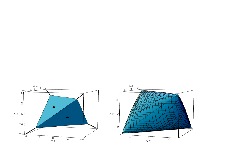
Figure 2: The fundamental domain (left) for constant gauge fields on $S^{3}$, with respect to the instanton framing $e_{\mu}^{a}$, in the “diagonal” representation $A_{a}=x_{a}\sigma_{a}$ (no sum over $a$). By the dots on the faces we indicate the sphalerons, whereas the dashed lines represent the symmetry axes of the tetrahedron. To the right we display the Gribov horizon, which encloses the fundamental domain, coinciding with it at the singular boundary points along the edges of the tetrahedron.

The (anti-)instantons in these framings are obtained from those for ${\rm I\kern-1.79993ptR}^{4}$ by identifying the radius in ${\rm I\kern-1.79993ptR}^{4}$ with the exponential of the time $t$ in the space $S^{3}\times{\rm I\kern-1.79993ptR}$. The (anti-)instanton that tunnels through the (anti-)sphaleron, has for each time a constant energy density, and is particularly simple with respect to this framing. One finds $A_{0}=0$, $A_{a}=A^{\mu}e_{\mu}^{a}=-f(t)\sigma_{a}$ for the instanton (and $A_{a}=A^{\mu}\bar{e}_{\mu}^{a}=-f(t)\sigma_{a}$ for the anti-instanton) with $f(t)=1/(1+e^{-2t})$. The (anti-)sphaleron occurs in this parametrisation at $t=0$. It is a saddle point of the energy functional with one unstable mode, corresponding to the direction of tunnelling. At $t=\infty$, $A_{a}=-\sigma_{a}$ has zero energy and is a gauge copy of $A_{a}=0$, by a gauge transformation $h=n\cdot\sigma^{\dagger}$ with winding number one. This gauge transformation also maps the anti-sphaleron to the sphaleron. The two dimensional space containing the tunnelling paths through the (anti-)sphalerons is parametrised by $A_{\mu}(u,v)={\scriptstyle{{1\over 2}}}(-ue^{a}_{\mu}-v\bar{e}^{a}_{\mu})\sigma_{a}$. The gauge transformation $h=n\cdot\sigma$ with winding number $-1$ is easily seen to map $(u,v)=(w,0)$ into $(u,v)=(0,2-w)$. The space of modes degenerate with these and of lowest energy is described by $A_{\mu}(c,d)=A_{i}(c,d)e_{\mu}^{i}={\scriptstyle{{1\over 2}}}(c^{a}_{i}e^{i}_{\mu}+d^{a}_{j}\bar{e}^{j}_{\mu})\sigma_{a}$. The $c$ and $d$ modes are mutually orthogonal and satisfy the Coulomb gauge condition $\partial_{i}A_{i}(c,d)=0$. The energy functional is given by [3]

$$\mbox{$\cal V$}(c,d) \equiv -\int_{S^{3}}\frac{1}{2}\mbox{\,tr\,}(F_{ij}^{2})=\mbox{$\cal V$}(c)+\mbox{$\cal V$}(d)+\frac{2\pi^{2}}{3}\left\{(c^{a}_{i})^{2}(d^{b}_{j})^{2}-(c^{a}_{i}d^{a}_{j})^{2}\right\},$$

$$\mbox{$\cal V$}(c) = 2\pi^{2}\left\{2(c^{a}_{i})^{2}+6\det c+\frac{1}{4}[(c^{a}_{i}c^{a}_{i})^{2}-(c^{a}_{i}c^{a}_{j})^{2}]\right\},$$ (4)

from which the degeneracy to second order in $c$ and $d$ can be verified. There are no modes with a lower zero-point frequency than these [13].

An effective Hamiltonian for the $c$ and $d$ modes is derived from the one-loop effective action [15]. To lowest order it is given by

$$H=-\frac{g^{2}(R)}{2R}\left(\left(\frac{\partial}{\partial c_{i}^{a}}\right)^{2}+\left(\frac{\partial}{\partial c_{i}^{a}}\right)^{2}\right)+\frac{1}{g^{2}(R)R}\mbox{$\cal V$}(c,d),$$ (5)

where $g(R)$ is the running coupling constant. It can be shown [13] that the boundary of the fundamental domain will touch the Gribov horizon $\partial\Omega$, such that it contains singular points. This is illustrated in figure 2, which shows the fundamental and Gribov regions for $d=0$, using the rotational and gauge invariance to rotate $c$ to a “diagonal” form.

It is essential that the sphalerons do not lie on the Gribov horizon and that the potential energy near $\partial\Omega$ is relatively high as can be seen from figure 1. This is why we can take the boundary identifications near the sphalerons into account without having to worry about singular boundary points, as long as the energies of the low-lying states will be not much higher than the energy of the sphaleron. It allows one to study the glueball spectrum as a function of the CP violating angle $\theta$, but more importantly it incorporates for $\theta=0$ the noticeable influence of the barrier crossings, i.e. of the instantons.

Figure 3: The full one-loop results for the masses of scalar, tensor and odd glueballs on $S^{3}$ as a function of $f=g^{2}(R)/2\pi^{2}$ for $\theta=0$. The dashed lines correspond to the perturbative result.

The boundary conditions are chosen so as to coincide with the appropriate boundary conditions near the sphalerons, but such that the gauge and (left and right) rotational invariances are not destroyed. Projections on the irreducible representations of these symmetries turned out to be essential to reduce the size of the matrices to be diagonalised in a Rayleigh-Ritz analysis. Remarkably all this could be implemented in a tractable way [15]. Results are summarised in figure 3. One of the most important features is that the $0^{-}$ glueball is (slightly) lighter than the $0^{+}$ in perturbation theory, but when including the effects of the boundary of the fundamental domain, setting in at $f\sim 0.2$, the $0^{-}/0^{+}$ mass ratio rapidly increases. Beyond $f\sim 0.28$ it can be shown that the wave functionals start to feel parts of the boundary of the fundamental domain which the present calculation is not representing properly [15]. This value of $f$ corresponds to a circumference of roughly 1.3 fm, when setting the scale as for the torus, assuming the scalar glueball mass in both geometries at this intermediate volume to coincide.

5 Conclusion

Boundary identifications become relevant at large volumes, whereas at very small volumes the wave functional is localised around $A=0$ and one need not worry about these non-perturbative effects. That these effects can be dramatic, even at relatively small volumes (above a tenth of a fermi across), was demonstrated for the case of the torus [1]. Here we have discussed the situation for $S^{3}$. Results for the spectrum are compatible with those of a torus in volumes around one fermi across [16], with $m(2^{+})/m(0^{+})\sim 1.5$ and $m(0^{-})/m(0^{+})\sim 1.7$. For more details and discussions see refs. [15, 17].

The author thanks the (session) organisers Yitzhak Frishman, Robert Perry, Simon Dalley and Pierre Grangé for their invitation. He also thanks the participants for many fruitful discussions on and off the slopes.

References

- [1] P. van Baal, Phys.Lett. 224B (1989) 397; Nucl. Phys. B351 (1991) 183.
- [2] M. Lüscher, Nucl.Phys. B219 (1983) 233
- [3] P. van Baal and N. D. Hari Dass, Nucl.Phys. B385 (1992) 185.
- [4] O. Babelon and C. Viallet, Comm.Math.Phys. 81 (1981) 515.
- [5] I. Singer, Comm.Math.Phys. 60 (1978) 7.
- [6] V. Gribov, Nucl.Phys. B139(1978) 1.
- [7] W. Nahm, in:IV Warsaw Sym.Elem.Part.Phys, 1981, ed. Z.Ajduk, p.275.
- [8] P. van Baal, in: Probabilistic Methods in Quantum Field Theory and Quantum Gravity, ed. P.H. Damgaard et al, (Plenum Press, New York, 1990) p31; Nucl.Phys. B(Proc.Suppl.)20 (1991) 3.
- [9] M.A. Semenov-Tyan-Shanskii and V.A. Franke, Zapiski Nauchnykh Seminarov Leningradskogo Otdeleniya Matematicheskogo Instituta im. V.A. Steklov AN SSSR, 120 (1982) 159. Translation: (Plenum Press, New York, 1986) p.999; D. Zwanziger, Nucl. Phys. B209 (1982) 336.
- [10] N.M. Christ and T.D. Lee, Phys.Rev. D22 (1980) 939.
- [11] G. Dell‘Antonio and D. Zwanziger, Nucl.Phys. B326 (1989) 333.
- [12] P. van Baal, Nucl.Phys. B369 (1992) 259.
- [13] P. van Baal and B. van den Heuvel, Nucl.Phys. B417 (1994) 215.
- [14] G. ’t Hooft, Phys.Rev. D14 (1976) 3432.
- [15] B.M van den Heuvel, Phys.Lett. B368 (1996) 124; B386 (1996) 233; Nucl.Phys. B488 (1997) 282.
- [16] C. Michael and M. Teper, Phys.Lett. B199 (1987) 95.
- [17] P. van Baal, Global issues in gauge fixing, in: ”Non-perturbative approaches to Quantum Chromodynamics”, ed. D. Diakonov, (Gatchina, 1995) p.4.