On the Role of the Annihilation Channel in Front Form Positronium

Abstract

The annihilation channel is implemented into the front form calculations of the positronium spectrum presented in Ref. [1]. The effective Hamiltonian is calculated analytically. Its eigensolutions are obtained numerically. A complete separation of the dynamical and instantaneous part of the annihilation interaction is observed. We find the remarkable effect that the annihilation channel stabilizes the cutoff behavior of the spectrum.

I Introduction

Recently, a calculation of the positronium spectrum within the front form formalism was presented [1]. In this work, the entire spectrum was calculated, i.e. all sectors defined by the kinetic component of the total angular momentum, $J_{z}$, were considered. However, the one photon annihilation channel was omitted. It is the purpose of the present paper to include this channel into the calculations, which are completed with this step.

The article is structured as follows. In Section II the implications of introducing the annihilation channel into the positronium theory are stated. Next, the spectrum of the “full” positronium is calculated and the results are presented. Section IV deals with the parameter dependence of the results, i.e. the dependence on cutoffs and convergence parameters. A discussion of the results follows. The calculation of the matrix elements of the effective Hamiltonian is reviewed in Appx. A.

II The annihilation channel in positronium

It is a topic of its own merit to construct a manageable Hamiltonian for the positronium system. One possible way was shown in Ref. [1], where an effective Fock space, consisting of two sectors $|e\bar{e}\rangle$ and $|e\bar{e}\gamma\rangle$, named $P$- and $Q$-space was considered. One can justify the absence of any higher Fock state [2] from the structure of the applied formalism of effective interactions [3]. The general formalism is set up for a non-abelian $SU(N)$ gauge theory. Unlike QED, the one boson state is absent in these theories because of color neutrality. Nevertheless, one has to take care of the one photon state $|\gamma\rangle$ in QED, and in what follows, we demonstrate how this can be done.

Firstly, it is important to notice not only the differences between the QED Table I and the analogous QCD table in [3], but also the similarities. Some of the graphs occuring in QCD are absent in QED. In particular those graphs with a three- or four-boson interaction and the instantaneous interactions connecting four bosons. But, although an additional sector occurs as a first row and a first column in the QED table, neither is a change in the higher Fock sectors observed, nor is the ordering altered in any way.

Sector

$n$

0

1

2

3

4

5

6

7

8

9

10

11

12

13

$|\gamma\rangle$

0

$\bullet$

V

$\cdot$

F

$\cdot$

$\cdot$

$\cdot$

$\cdot$

$\cdot$

$\cdot$

$\cdot$

$\cdot$

$\cdot$

$\cdot$

$|e\bar{e}\rangle$

1

V

$\bullet$

S

V

F

$\cdot$

F

$\cdot$

$\cdot$

$\cdot$

$\cdot$

$\cdot$

$\cdot$

$\cdot$

$|\gamma\ \gamma\rangle$

2

$\cdot$

S

$\bullet$

V

$\cdot$

V

F

$\cdot$

$\cdot$

$\cdot$

$\cdot$

$\cdot$

$\cdot$

$\cdot$

$|e\bar{e}\,\ \gamma\rangle$

3

F

V

V

$\bullet$

V

S

V

F

$\cdot$

$\cdot$

$\cdot$

$\cdot$

$\cdot$

$\cdot$

$|e\bar{e}\,e\bar{e}\rangle$

4

$\cdot$

F

$\cdot$

V

$\bullet$

$\cdot$

S

V

F

$\cdot$

$\cdot$

F

$\cdot$

$\cdot$

$|\gamma\ \gamma\ \gamma\rangle$

5

$\cdot$

$\cdot$

V

S

$\cdot$

$\bullet$

V

$\cdot$

$\cdot$

V

F

$\cdot$

$\cdot$

$\cdot$

$|e\bar{e}\,\ \gamma\ \gamma\rangle$

6

$\cdot$

F

F

V

S

V

$\bullet$

V

$\cdot$

S

V

F

$\cdot$

$\cdot$

$|e\bar{e}\,e\bar{e}\,\ \gamma\rangle$

7

$\cdot$

$\cdot$

$\cdot$

F

V

$\cdot$

V

$\bullet$

V

$\cdot$

S

V

F

$\cdot$

$|e\bar{e}\,e\bar{e}\,e\bar{e}\rangle$

8

$\cdot$

$\cdot$

$\cdot$

$\cdot$

F

$\cdot$

$\cdot$

V

$\bullet$

$\cdot$

$\cdot$

S

V

F

$|\gamma\ \gamma\ \gamma\ \gamma\rangle$

9

$\cdot$

$\cdot$

$\cdot$

$\cdot$

$\cdot$

V

S

$\cdot$

$\cdot$

$\bullet$

V

$\cdot$

$\cdot$

$\cdot$

$|e\bar{e}\,\ \gamma\ \gamma\ \gamma\rangle$

10

$\cdot$

$\cdot$

$\cdot$

$\cdot$

$\cdot$

F

V

S

$\cdot$

V

$\bullet$

V

$\cdot$

$\cdot$

$|e\bar{e}\,e\bar{e}\,\ \gamma\ \gamma\rangle$

11

$\cdot$

$\cdot$

$\cdot$

$\cdot$

F

$\cdot$

F

V

S

$\cdot$

V

$\bullet$

V

$\cdot$

$|e\bar{e}\,e\bar{e}\,e\bar{e}\,\ \gamma\rangle$

12

$\cdot$

$\cdot$

$\cdot$

$\cdot$

$\cdot$

$\cdot$

$\cdot$

F

V

$\cdot$

$\cdot$

V

$\bullet$

V

$|e\bar{e}\,e\bar{e}\,e\bar{e}\,e\bar{e}\rangle$

13

$\cdot$

$\cdot$

$\cdot$

$\cdot$

$\cdot$

$\cdot$

$\cdot$

$\cdot$

F

$\cdot$

$\cdot$

$\cdot$

V

$\bullet$

TABLE I.: The Hamiltonian matrix for QED. The sectors $n$ are numbered starting at zero. The vertex, seagull and fork interactions are denoted by V, S, F respectively. Diagonal matrix elements are symbolized by $\bullet$.

In addition to the $P$- and $Q$-spaces defined above, we introduce the $N$-space, i.e. the sector containing the $|\gamma\rangle$ states, into the system. The corresponding projector is

$$\hat{N}:=\sum_{n}^{\rm all\;\;QN}|(\gamma)_{n}\rangle\langle(\gamma)_{n}|.$$ (1)

The whole procedure of subsequent projections of higher Fock states onto the remaining Hilbert space of states can be carried out like before [1] until one arrives at a $(2\times 2)$ matrix, operating in the $N$- and $P$-space rather than in the $P$- and $Q$-space

$$H_{\rm LC}\;\psi=\left(\begin{array}[]{cc}H_{NN}&H_{NP}\\ H_{PN}&H_{PP}\\ \end{array}\right)\left(\begin{array}[]{c}\psi_{\gamma}\\ \psi_{e\bar{e}}\\ \end{array}\right)=\omega\left(\begin{array}[]{c}\psi_{\gamma}\\ \psi_{e\bar{e}}\\ \end{array}\right).$$ (2)

From Table I one can read off the interaction of the one photon state with all other sectors: the vertex interaction annihilates the photon into an electron-positron pair and a fork interaction scatters it into the sector $|e\bar{e}\gamma\rangle$. The latter interaction is already contained in the effective interaction, Eq. (2), because of the projection of the $Q$-space.

FIG. 1.: The positronium spectrum including the annihilation channel in the $J_{z}{=}0$ sector. Parameters of the calculation: $\alpha=0.3,\Lambda=1.0\,m_{f}$. The mass squared eigenvalues $M^{2}_{n}$ in units of the electron mass $m^{2}_{f}$ are shown as functions of the number of integration points $N\equiv N_{1}=N_{2}$. The triplet states, especially $1^{3}S_{1}$, are lifted up by the annihilation interaction, whereas the singlet mass eigenvalues stay the same.

	=		+
	+
	+		+

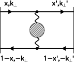
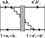
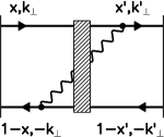
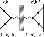
FIG. 2.: The graphs of the positronium model. Effective photon lines are labelled by hashed rectangles. The graphs of the annihilation interaction are at the bottom line.

Although we projected the higher Fock sectors onto the lower ones to construct the effective interaction up to now, one is, of course, free to project the (lower) $|\gamma\rangle$-sector onto the (higher) $|e\bar{e}\rangle$-sector, and obtains

$$H_{\rm eff}(\omega)=H_{PP} + H_{PN}\frac{1}{\omega-H_{NN}}H_{NP}$$ (3)

$$+ H_{PQ}\frac{1}{\omega-H_{QQ}}H_{QP}$$ (4)

Of course we do this for convenience; we could just as well solve the eigenvalue problem of Eq. (2). The projection is depicted in the two graphs in the bottom line of Fig. 2. One is the dynamic annihilation graph, the other is the corresponding seagull annihilation graph. The latter is a $P$-space graph and was omitted in Ref. [1] following the gauge principle of Tang [4].

III Spectrum including the annihilation channel

The spectrum including the annihilation channel shows the expected properties: the singlet eigenvalues remain unchanged, while the triplet states change. An essential point in the actual calculations is that one has to use the same counterterms for the Coulomb singularity as used without the annihilation channel. This is due to the fact that the one photon annihilation part of the interaction has no additional singularity that needs to be taken care of numerically, because of the simple energy denominator, Eq. (A2). We compiled our results in the form of binding coefficients in Table III.

FIG. 3.: Deviation of corresponding eigenvalues for $J_{z}{=}0$ and $J_{z}{=}1$ including the annihilation channel as a function of the number of integration points $N$ for $\alpha{=}0.3$, $\Lambda{=}1.0\,m_{f}$. The graph shows $\Delta M^{2}{:=}$ $M^{2}_{n}(J_{z}=0)-M^{2}_{n}(J_{z}=1)$ for the states $1^{3}S_{1}\,(\triangle)$, $2^{3}P_{1}\,(\Box)$, and $2^{1}P_{1}\,(\circ)$.

One notes a slightly larger breaking of rotational symmetry as in the case of missing annihilation channel. The triplet ground states of different $J_{z}$ are still degenerate to a very good approximation, but the discrepancy is bigger than without the annihilation channel. The dependence of these discrepancies between corresponding eigenvalues for $J_{z}{=}0$ and $J_{z}{=}1$ on the number of integration points is shown in Fig. 3. The behavior of the curves is similar to those of the calculations without annihilation channel, cf. Fig. 13 of Ref. [1]. An additional plot, Fig. 3, shows the dependence of the rotational symmetry breaking on the cutoff $\Lambda$. The discrepancies of corresponding eigenvalues are almost independent of the cutoff $\Lambda$.

FIG. 4.: Deviation of corresponding eigenvalues for $J_{z}{=}0$ and $J_{z}{=}1$ including the annihilation channel as a function of the cutoff $\Lambda$ for $\alpha{=}0.3,\Lambda{=}1.0\,m_{f}$. The graph shows $\Delta M^{2}:=M^{2}_{n}(J_{z}{=}0)-M^{2}_{n}(J_{z}{=}1)$ for the states $1^{3}S_{1}\,(\triangle)$, $2^{3}P_{1}\,(\Box)$, and $2^{1}P_{1}\,(\circ)$.

To make a comparison of our results to those of perturbation theory easier, we show in Fig. 10 the values for the principal quantum number $n{=}2$ for both theories graphically. The structure of the two plots is almost the same, only the $2^{1}S_{0}$ state and the $2^{3}P_{0}$ state are exchanged in our results. This is due to the cutoff dependence of the S-state, which is larger than that of the other states (cf. Fig. 5(b) and next paragraph). We stress that the results of the perturbative calculations change considerably, when the next higher order in $\alpha$ is considered. For example, the mass squared of the triplet $2^{3}S_{1}$ is, according to Fulton and Martin [5], $M^{2}(2^{3}S_{1})=3.9780186070$ up to order $\alpha^{3}{Ry\;}$, which is nearer to our result than the value of perturbative calculations up to order ${\cal O}(\alpha^{4})$, displayed in Fig. 10. $\mbox{Cutoff: }\Lambda$ $B_{s}$ $B_{t}$ $C_{hf}$ 1.8 1.16373904 0.96234775 0.55942025 3.6 1.25570163 0.96446614 0.80898748 5.4 1.29978067 0.96482118 0.93044303 7.2 1.32941926 0.96541695 1.01111752 9.0 1.35224000 0.96603457 1.07279285 10.8 1.37112216 0.96661006 1.12364471 12.6 1.38744792 0.96713137 1.16754595 14.4 1.40198469 0.96760110 1.20662108 16.2 1.41520247 0.96802548 1.24215830 18.0 1.42740143 0.96841025 1.27497551 ETPT 1.11812500 0.90812500 0.58333333 ${\cal O}(\alpha^{6}\ln\alpha)$ 0.48792985 TABLE II.: The binding coefficients of the singlet ($B_{s}$), the triplet ($B_{t}$), and the hyperfine coefficient $C_{hf}$ are listed for $\alpha=0.3,$ $N_{1}=41,N_{2}=11$. For a comparison, the coefficients of equal time perturbation theory are also listed, up to order ${\cal O}(\alpha^{4})$ (ETPT) and to ${\cal O}(\alpha^{6}\ln\alpha)$

IV Parameter dependence of the spectrum

The convergence of the eigenvalues with growing number of integration points $N$ is the same as the case of no annihilation channel. To be explicit, the convergence of the eigenvalues can be shown to be exponential. We performed a $\chi^{2}$ fit to the function

$$f(N)=a-b\exp\left\{(N-N_{0})/c\right\}.$$ (5)

and obtain for the singlet ground state $1\,^{1\!}S_{0}$ $a=3.9061000\pm 0.0000008$, $b=(9.6399\pm 0.0193)\times 10^{-4},$ and $c=2.2372\pm 0.0063,$ with $\chi^{2}=5.7$. We did not perform the limit $N\rightarrow\infty$, because the accuracy of the results for $N>20$ suffices to compare to other data.

The cutoff dependence of the positronium spectrum including the annihilation channel is comparable to that of the spectrum without it. However, a striking difference occurs: the inclusion of the annihilation channel stabilizes the cutoff dependence of the eigenstates. In particular, the triplet ground state in Fig. 5(a) shows only a small dependence on the cutoff, when one compares it to the behavior of the same state in the calculations without annihilation channel [1]. One can fit these curves with a polynomial in $\log\Lambda$. The singlet ground state eigenvalues are the same as without the annihilation graph and for the triplet one obtains

$$M^{2}_{t}(\Lambda)\simeq 3.91392-0.00029\log\Lambda+0.00015\log^{2}\Lambda.$$ (6)

Comparison with Eq. (22) of Ref. [1] shows that the decrease of the triplet with $\log\Lambda$ is suppressed by including the annihilation channel by a factor of 60. Also the excited states, $n{=}2$, show a different behavior, when compared to Fig. 13 of Ref. [1]. Here, only one state shows level crossing as $\Lambda$ grows large. The eigenvalue of the $2^{3}P_{1}$ state, however, depends only weakly on the cutoff.

FIG. 5.: The spectrum with annihilation channel as a function of the cutoff $\Lambda$: ground states ($n{=}1$). The parameters for the calculation are $\alpha=0.3$, $J_{z}=0$, $N_{1}=25$, $N_{2}=21$.

FIG. 6.: The spectrum with annihilation channel as a function of the cutoff $\Lambda$: first radial excited states ($n{=}2$). The parameters for the calculation are $\alpha=0.3$, $J_{z}=0$, $N_{1}=25$, $N_{2}=21$.

The values for the binding coefficients $B_{n}$ and the coefficient of the hyperfine splitting $C_{hf}$ are presented in Table II. The values are correct for a cutoff $\Lambda\simeq 2m_{f}$ when compared to results of perturbation theory up to ${\cal O}(\alpha^{4})$. However, the effects of higher order correction to perturbative calculations are significant for a large coupling such as $\alpha=0.3$. The result of perturbation theory to ${\cal O}(\alpha^{6}\ln\alpha)$ for the coefficient $C_{hf}$ is considerably smaller than that to order ${\cal O}(\alpha^{4})$.

Concluding, we state that the cutoff dependence of the spectrum is improved as compared with the case of missing annihilation channel. This makes it evident that the annihilation channel is a necessary part of the theory. Note that in muonium, the annihilation state is absent. This can lead to problems in interpreting the stabilizing feature of the channel [6].

As a further investigation of the properties of our model, we will vary the coupling constant and interpret the spectrum. A similar procedure was performed by Dykshoorn et al. [7, 8], who studied coupled integral equations for QED-bound states in equal-time quantization with a variational ansatz. They calculate masses for the lowest eigenstates of positronium with and without the annihilation channel and plot them versus the coupling constant. The prominent feature of their figures is the occurrence of a critical coupling at which the masses become smaller than zero. We have performed the analogous calculations within our approach. It seems at first glance [Fig. 8(a)] as if the eigenvalues, after decreasing quadratically with the coupling as expected by perturbation theory, stabilize at a coupling $\alpha\simeq 1.5$. However, further investigation shows that this is merely an effect of the cutoff dependence of the spectrum. The eigenvalues in Fig. 8(a) were calculated with a cutoff $\Lambda=1.0\;m_{f}$, which is too small for a coupling constant of $\alpha=1.0$, since then the Bohr momentum is of the same order as the cutoff. Fig. 8(b) shows clearly that there is a critical coupling. The masses calculated with a cutoff of $\Lambda=20\,m_{f}$ tend to zero at $\alpha\simeq 0.5$. A similar value was found in [8].

V Discussion

In the present work we completed in a sense the theory of positronium in front form dynamics set up in Ref. [1]. The theory was enlarged by including the one photon annihilation channel. The inclusion is a test for the consistency of the model. In particular, the conception of an effective theory operating with resolvents can be falsified if the annihilation channel cannot be implemented without special assumptions. Our results show that the implementation of the annihilation channel is unproblematic in the sense that the same formalism can be applied as in the case of the projection of the effective $|e\bar{e}\gamma\rangle$-sector onto the electron-positron sector. As an interesting property of the annihilation channel we find a strict separation of the instantaneous and the non-instantaneous interaction: the seagull interaction is present only in the $J_{z}=0$ sector, whereas the dynamic graph has non-vanishing matrix elements only for $J_{z}=\pm 1$. Our approach passes another test: both graphs yield the same contributions to the eigenvalues and consequently rotational symmetry is seen also in the spectrum including the annihilation channel. Moreover, the inclusion of the annihilation channel improves the results for the hyperfine splitting.

We stress the point that the implementation of the annihilation channel completes the investigations of how to construct an effective interaction for the electromagnetic fermion-antifermion system in the meaning of the method of iterated resolvents. We have put all effects of higher Fock states into an effective $|e\bar{e}\gamma\rangle$-sector, as far as the spectator interaction is concerned, i.e. the interactions in which the photons are not directly involved. The remainder of the interaction relies in the coupling function of the vertices. A hint to this conclusion is the logarithmic cutoff dependence of our results. It is clear that the coupling constant depends on the cutoff and has to be analyzed. A future aim, beyond the scope of this work, will be to show that the physical results of our model become independent of the cutoff, as soon as renormalization group techniques are consistently applied. This is supported by the fact that we find a stabilizing effect of the annihilation channel on the dependence of the spectrum on the cutoff: all eigenvalues show slower variation with growing cutoff $\Lambda$ when the annihilation graph is added, in some cases this even prevents level crossings with other states. However, in muonium for instance, this channel is absent and it remains unclear which interpretation this should yield. We therefore conclude that our model is correct as long as the vacuum polarization effects are not considered.

The possibility of one boson annihilation is the main difference between QED and QCD in effectively truncated Fock spaces where the dynamic three- or four-gluon interaction is not possible but resides in the coupling function. The one boson sector exists only in QED because of the constraint of color neutrality in QCD. We showed that this sector can be projected onto the (already) effective electron-positron sector.

$n$	Term	$\hfill B_{n}(J_{z}{=}0)\hfill$	$\hfill B_{n}(J_{z}{=}+1)\hfill$	$\hfill\Delta B_{n}\hfill$
1	$1^{1}S_{0}$	1.049552(17)	—	—
2	$1^{3}S_{1}$	0.936800(189)	0.937902(151)	-0.001102
3	$2^{1}S_{0}$	0.260237(169)	—	—
4	$2^{3}S_{1}$	0.255292(184)	0.255359(179)	-0.000067
5	$2^{1}P_{1}$	0.257969(160)	0.258037(168)	-0.000068
6	$2^{1}P_{1}$	0.267090(160)	—	—
7	$2^{3}P_{1}$	0.259667(206)	0.260013(163)	-0.000346
8	$2^{3}P_{2}$	0.245615(239)	0.245755(228)	-0.000140
9	$3^{1}S_{0}$	0.115206(314)	—	—
10	$3^{3}S_{1}$	0.113434(156)	0.113497(179)	-0.000063
11	$3^{1}P_{1}$	0.114490(269)	0.114521(283)	-0.000032
12	$3^{1}P_{1}$	0.117142(272)	—	—
13	$3^{3}P_{1}$	0.115127(326)	0.115102(275)	0.000025
14	$3^{3}P_{2}$	0.113731(284)	0.113753(283)	-0.000023
15	$3^{1}D_{2}$	0.112816(150)	0.112842(158)	-0.000027
16	$3^{3}D_{1}$	0.112977(161)	0.112987(164)	-0.000010
17	$3^{3}D_{2}$	0.112520(158)	0.112524(160)	-0.000004
18	$3^{3}D_{3}$	0.111027(377)	0.111072(373)	-0.000045
19	$4^{1}S_{0}$	0.065490(588)	—	—
20	$4^{3}S_{1}$	0.064707(480)	0.064723(481)	-0.000016
21	$4^{1}P_{1}$	0.065003(467)	0.065061(486)	-0.000059
22	$4^{1}P_{1}$	0.066119(470)	—	—
23	$4^{3}P_{1}$	0.065331(487)	0.065276(475)	0.000055
24	$4^{3}P_{2}$	0.064265(309)	0.064372(348)	-0.000107
25	$4^{1}D_{2}$	0.063968(430)	0.064041(363)	-0.000073
26	$4^{3}D_{1}$	0.064099(319)	0.064090(325)	0.000009
27	$4^{3}D_{2}$	0.063870(391)	0.063881(477)	-0.000011
28	$4^{3}D_{3}$	0.063788(387)	0.063807(381)	-0.000019
29	$4^{1}F_{3}$	0.063141(96)	0.063112(104)	0.000030
30	$4^{3}F_{2}$	0.063299(112)	0.063233(116)	0.000065
31	$4^{3}F_{3}$	0.063234(119)	0.063209(119)	0.000024
32	$4^{3}F_{4}$	0.063103(104)	0.063422(158)	-0.000319
33	$5^{1}S_{0}$	0.043253(806)	—	—
34	$5^{3}S_{1}$	0.043046(682)	0.042912(739)	0.000134
35	$5^{1}P_{1}$	0.043412(1100)	0.042724(853)	0.000688

TABLE III.: The positronium spectrum for $\alpha=0.3,$ $\Lambda=1.0\,m_{f},N_{1}=N_{2}=21$. The non-relativistic notation for the terms and the binding coefficients $B_{n}:=(4-M_{n})/\alpha^{2}$ for $J_{z}{=}0$ and $J_{z}{=}+1$ including the annihilation channel are shown. The discrepancy between the eigenvalues is $\Delta B_{n}:=B_{n}(J_{z}{=}0)-B_{n}(J_{z}{=}+1)$. The numerical errors are estimated from the difference between the values for maximum and next to maximum number of integration points. The actual errors are smaller due to the exponential convergence of the eigenvalues with $N$. The $k$ numbers in brackets are the errors in the last $k$ digits.

FIG. 7.: Compiled spectra of positronium with different $J_{z}=-3,-2,\ldots,+3$ including the annihilation channel. All spectra have been calculated with $\alpha=0.3$, $\Lambda=1.0\,m_{f}$, $N_{1}=N_{2}=21$. The mass squared eigenvalues $M^{2}_{n}$ in units of the electron mass $m^{2}_{f}$ are shown. The notation for the states is ${}^{3S+1}L^{J_{z}}_{J}$. The resolution of the plot is inadequate for the multiplets. Nevertheless, the numerical degeneracy of the three triplet ground states ${}^{3}S^{-1}_{1}$,${}^{3}S^{0}_{1}$, and ${}^{3}S^{1}_{1}$ becomes very clear.

FIG. 8.: The spectrum as a function of the coupling constant for $\Lambda=1.0\,m_{f}$. Here, the eigenvalues seem to converge to a stable value as $\alpha$ grows large. However, this is just an effect of the cutoff dependence of the spectrum: for a larger cutoff $\Lambda=20\,m_{f}$ the eigenvalues become negative at a critical coupling $\alpha_{c}\simeq 0.5$.

FIG. 9.: The spectrum as a function of the coupling constant for $\Lambda=20.0\,m_{f}$. For this large cutoff the eigenvalues become negative at a critical coupling $\alpha_{c}\simeq 0.5$.

A Calculation of effective matrix elements

The implementation of the annihilation channel is straightforward, but non-trivial. We describe shortly the calculation in the $(J_{z}{=}0)$ and $(J_{z}{=}\pm 1)$ sectors. The corresponding diagrams, displayed in the lowest line of Fig. 2, vanish in all other sectors because of the helicity of the photon: no angular momentum larger than $J=1$ is possible. The functions derived depend on the light-cone momenta, $(x,\,\vec{k}_{\perp})$, and are given in Table V. They have to be added to the functions listed in Ref. [1], Table V, to obtain the full Hamiltonian. Following the procedure described in Ref. [1] (cf. also Ref. [9]), we use for the energy denominator the following averaged kinetic energy

$$T^{*}(x,\vec{k}_{\perp};x^{\prime},\vec{k}^{\prime}_{\perp})=\frac{1}{2}\left(\frac{m_{f}^{2}+\vec{k}_{\perp}}{x(1-x)}+\frac{m_{f}^{2}+\vec{k}^{\prime}_{\perp}}{x^{\prime}(1-x^{\prime})}\right).$$ (A1)

The denominator in the one photon sector is simple because the photon has zero mass:

$$G(\omega)=\frac{1}{\omega-H_{\gamma}}=\frac{1}{T^{*}}.$$ (A2)

Note that this denominator does not depend on the directions of the vectors $\vec{k}_{\perp}$, $\vec{k}_{\perp}^{\prime}$, i.e. on the angles $\varphi$, $\varphi^{\prime}$.

The matrix elements of the vertex interaction $V_{g\rightarrow q\bar{q}}$ (cf. e.g. Ref. [10]) split up into their three components with different helicity factors, are

$$\langle e\bar{e}|V_{A}|\gamma\rangle = -m\sqrt{\beta}\frac{1}{x(1-x)}\times\delta^{+\lambda_{1}}_{+\lambda_{2}}\delta^{+\lambda_{1}}_{+\lambda_{3}},$$ (A3)

$$\langle e\bar{e}|V_{B}|\gamma\rangle = -\sqrt{\beta}\frac{k_{\perp}}{1-x}e^{+i\lambda_{2}\varphi}\times\delta^{+\lambda_{1}}_{+\lambda_{2}}\delta^{+\lambda_{1}}_{-\lambda_{3}},$$ (A4)

$$\langle e\bar{e}|V_{C}|\gamma\rangle = \sqrt{\beta}\frac{k_{\perp}}{x}e^{-i\lambda_{2}\varphi}\times\delta^{+\lambda_{1}}_{-\lambda_{2}}\delta^{+\lambda_{1}}_{+\lambda_{3}}.$$ (A5)

The complete matrix elements are obtained by symmetry, since $\langle e\bar{e}|V_{i}|\gamma\rangle=\overline{\langle\gamma|V_{i}|e\bar{e}\rangle}.$ To classify the states according to their quantum numbers with respect to the third (kinetic) component of the total angular momentum, ${\cal J}_{3}$, we project on sectors of definite $J_{z}$. It turns out that because of the simple energy denominator, Eq. (A2), the only dependence on the angles comes from the projectors on the $J_{z}$ sectors and is proportional to $\cos\{\varphi-\varphi^{\prime}\}$ or $\sin\{\varphi-\varphi^{\prime}\}$. As a result, all matrix elements of the dynamic annihilation graph for $J_{z}{=}0$ vanish when integrated over the angles. Only for $J_{z}{=}\pm 1$ do some of the matrix elements survive the integration.

Because of the combination of matrix elements with the projectors onto the $J_{z}$ sectors, two types of functions emerge for $J_{z}{=}\pm 1$: one is independent of the angles, the other has a dependence proportional to $\exp\{\pm 2i(\varphi-\varphi^{\prime})\}$. The latter vanishes after angular integration. The helicity table IV is given to illustrate the helicity dependencies. It holds for $J_{z}{=}+1$. The analogous table for $J_{z}{=}-1$ is obtained by the operation

$\displaystyle W_{ij}(J_{z}{=}\!+\!1;\,\lambda_{1},\lambda_{2})=-\lambda_{1}W_{ij}(J_{z}{=}\!-\!1;\,-\lambda_{1},-\lambda_{2}).$

The simple kinematics ($x_{e}+x_{\bar{e}}=1$) of the seagull annihilation graph result in a constant contribution of this graph to the Hamiltonian matrix. It is

$$\langle e\bar{e}|S|e\bar{e}\rangle=-2\beta\delta^{+\lambda_{2}}_{-\lambda_{1}}\times\delta^{+\lambda_{2}^{\prime}}_{-\lambda_{1}^{\prime}}.$$ (A6)

Because of its helicity factors, the graph acts only between states with

$$S_{z}=S_{z}^{\prime}=0.$$ (A7)

This means that the seagull graph does not contribute when $J_{z}{\neq}0$, because it has a factor proportional to $\cos(\varphi-\varphi^{\prime})$ resulting from (A7). A rather surprising consequence is that the dynamic graph contributes only for $J_{z}=\pm 1$, the instantaneous graph only for $J_{z}=0$. However, to maintain rotational invariance, both diagrams must yield the same value, though one shows much more structure than the other. Degeneracy of the orthopositronium ground state with respect to $J_{z}$ is found without the annihilation channel and inclusion must not destroy it. At first glance, there seems to be a manifest breaking of rotational symmetry: the helicity table IV separates between states with $(\lambda_{1},\lambda_{2})=(\uparrow\uparrow)$ and $(\lambda_{1},\lambda_{2})=(\downarrow\downarrow)$. But this is only a consequence of the integration over the angles: for $J_{z}=+1$ the $(\downarrow\downarrow)$- combination gives no contribution, and likewise does the $(\uparrow\uparrow)$-combination for $J_{z}=-1$.

out : in	$\lambda_{1}^{\prime},\lambda_{2}^{\prime}=\uparrow\uparrow$	$\lambda_{1}^{\prime},\lambda_{2}^{\prime}=\uparrow\downarrow$	$\lambda_{1}^{\prime},\lambda_{2}^{\prime}=\downarrow\uparrow$	$\lambda_{1}^{\prime},\lambda_{2}^{\prime}=\downarrow\downarrow$
$\lambda_{1},\lambda_{2}=\uparrow\uparrow$	$W_{AA}$	$W_{AB}$	$W_{AC}$	$0$
$\lambda_{1},\lambda_{2}=\uparrow\downarrow$	$W_{BA}$	$W_{BB}$	$W_{BC}$	$0$
$\lambda_{1},\lambda_{2}=\downarrow\uparrow$	$W_{CA}$	$W_{CB}$	$W_{CC}$	$0$
$\lambda_{1},\lambda_{2}=\downarrow\downarrow$	$0$	$0$	$0$	$0$

TABLE IV.: Symbolic helicity table for the dynamic annihilation graph. The functions $W_{ii}$ are identical with the expressions $F_{i}$ listed in Table V. Here, terms proportional to $\delta_{|J_{z}|,0}$ are omitted.

The dependence of the effective interaction on the helicities of in- and out-going particles is displayed in the form of tables. The following notation is used for functions of the type $F(x,k_{\perp};x^{\prime},k_{\perp}^{\prime})$. An asterisk denotes the permutation of particle and anti-particle

$\displaystyle F_{3}^{*}(x,k_{\perp};x^{\prime},k_{\perp}^{\prime}):=F_{3}(1-x,-k_{\perp};1-x^{\prime},-k_{\perp}^{\prime}).$If the function additionally depends on the component of the total angular momentum $J_{z}=n$, a tilde symbolizes the operation $\tilde{F}_{i}(n)=F_{i}(-n)$.

1 Helicity table of the annihilation graph

The functions $F_{i}(1;2):=F_{i}(x,k_{\perp};x^{\prime},k_{\perp}^{\prime})$ displayed in Table V are:

$$F_{1}(x,k_{\perp};x^{\prime},k_{\perp}^{\prime}) := \frac{\alpha}{\pi}\frac{2}{\omega^{*}}\frac{m^{2}}{xx^{\prime}(1-x)(1-x^{\prime})}\delta_{|J_{z}|,1}$$

$$F_{2}(x,k_{\perp};x^{\prime},k_{\perp}^{\prime}) := \frac{\alpha}{\pi}\left(\frac{2}{\omega^{*}}\frac{k_{\perp}k_{\perp}^{\prime}}{xx^{\prime}}\delta_{|J_{z}|,1}+4\delta_{J_{z},0}\right)$$

$$F_{3}(x,k_{\perp};x^{\prime},k_{\perp}^{\prime}) := \frac{\alpha}{\pi}\frac{2}{\omega^{*}}\lambda_{1}\frac{m}{x(1-x)}\frac{k_{\perp}^{\prime}}{1-x^{\prime}}\delta_{|J_{z}|,1}$$

$$F_{4}(x,k_{\perp};x^{\prime},k_{\perp}^{\prime}) := -\frac{\alpha}{\pi}\left(\frac{2}{\omega^{*}}\frac{k_{\perp}k_{\perp}^{\prime}}{x^{\prime}(1-x)}\delta_{|J_{z}|,1}-4\delta_{J_{z},0}\right).$$

The table for $J_{z}=-1$ is obtained by inverting all helicities. Note that the table has non-vanishing matrix elements for $|J_{z}|\leq 1$ only. This restriction is due to the angular momentum of the photon.

out:in	$\lambda^{\prime}_{1}\lambda^{\prime}_{2}=\uparrow\uparrow$	$\lambda^{\prime}_{1}\lambda^{\prime}_{2}=\uparrow\downarrow$	$\lambda^{\prime}_{1}\lambda^{\prime}_{2}=\downarrow\uparrow$	$(\lambda^{\prime}_{1},\lambda^{\prime}_{2}=\downarrow\downarrow$
$\lambda_{1}\lambda_{2}=\uparrow\uparrow$	$F_{1}(1;2)$	$F_{3}(2;1)$	$F^{*}_{3}(2;1)$	$0$
$\lambda_{1}\lambda_{2}=\uparrow\downarrow$	$F_{3}(1;2)$	$F^{*}_{2}(1;2)$	$F_{4}(2;1)$	$0$
$\lambda_{1}\lambda_{2}=\downarrow\uparrow$	$F_{3}^{*}(1;2)$	$F_{4}(1;2)$	$F_{2}(1;2)$	$0$
$\lambda_{1}\lambda_{2}=\downarrow\downarrow$	$0$	$0$	$0$	$0$

TABLE V.: Helicity table of the annihilation graph for $J_{z}\geq 0$.

FIG. 10.: Comparison of multiplets for $n{=}2$: (a) results of the present work with $\alpha=0.3$, $\Lambda=1.0\,m_{f}$, $N_{1}=N_{2}=21$; (b) equal-time perturbation theory (ETPT) up to order ${\cal O}(\alpha^{4})$.

REFERENCES

- [1] U. Trittmann and H.-C. Pauli, On rotational invariance in front form dynamics, 1997, hep-th/9705021.
- [2] Or rather the substitution of effects of higher Fock sectors with the use of effective matrix elements in the remaining sectors.“Higher” here in the sense of ascending in Table I.
- [3] H.-C. Pauli, Solving Gauge field Theory by Discretized Light-Cone Quantization, 1996, hep-th/9608035.
- [4] A. C. Tang, S. J. Brodsky, and H.-C. Pauli, Phys. Rev. D 44, 1842 (1991).
- [5] T. Fulton and P. Martin, Phys. Rev. 95, 811 (1954).
- [6] S. J. Brodsky, private communication.
- [7] W. Dykshoorn and R. Koniuk, Phys. Rev. A 41, 60 (1990).
- [8] W. Dykshoorn and R. Koniuk, Phys. Rev. A 41, 64 (1990).
- [9] U. Trittmann and H.-C. Pauli, Quantum electrodynamics at strong couplings, 1997, hep-th/9704215.
- [10] A. Tang, S. J. Brodsky, and H.-C. Pauli, Phys. Rev. D 44, 1842 (1991).