hep-th/9704169

CERN-TH/97-58

CTP-TAMU-22/97

ACT-07/97

OUTP-97–16P

Quantum Decoherence in a $D$-Foam Background
John Ellis^a, N.E. Mavromatos^b,⋄, D.V. Nanopoulos^c,d,e
Abstract

Within the general framework of Liouville string theory, we construct a model for quantum $D$-brane fluctuations in the space-time background through which light closed-string states propagate. The model is based on monopole and vortex defects on the world sheet, which have been discussed previously in a treatment of $1+1$-dimensional black-hole fluctuations in the space-time background, and makes use of a $T$-duality transformation to relate formulations with Neumann and Dirichlet boundary conditions. In accordance with previous general arguments, we derive an open quantum-mechanical description of this $D$-brane foam which embodies momentum and energy conservation and small mean energy fluctuations. Quantum decoherence effects appear at a rate consistent with previous estimates.

^a Theory Division, CERN, CH-1211, Geneva, Switzerland,
^b University of Oxford, Dept. of Physics (Theoretical Physics), 1 Keble Road, Oxford OX1 3NP, United Kingdom,
^c Center for Theoretical Physics, Dept. of Physics, Texas A & M University, College Station, TX 77843-4242, USA,
^d Astroparticle Physics Group, Houston Advanced Research Center (HARC), The Mitchell Campus, Woodlands, TX 77381, USA.
^e Academy of Athens, Chair of Theoretical Physics, Division of Natural Sciences, 28 Panepistimiou Avenue, Athens 10679, Greece.
^⋄ P.P.A.R.C. Advanced Fellow.

CERN-TH/97-58

CTP-TAMU-22/97

ACT-07/97

OUTP-97-16P

April 1997

Our objective in this paper is to set up a formalism suitable for describing the propagation of a low-energy light particle, interpreted as a closed string state, through a fluctuating quantum space-time background, for which we adapt and develop emergent $D$-brane technology. The physical question towards which this study is directed is whether conventional quantum mechanics can be maintained in the presence of such a space-time foam. Hawking has argued [1] that a quantum state propagating through such a fluctuating background inevitably decoheres in general, as a result of information loss through Planck-scale event horizons. His arguments were based heuristically on model calculations in a quantum treatment of a conventional field-theoretical gravity [1, 2]. We have made similar arguments [3] and developed an appropriate open quantum-mechanical treatment of the evolution of a microscopic system, using as a guide a $(1+1)$-dimensional string black-hole model [4].

We argued that, whilst the Hawking-Bekenstein black-hole entropy was given by the number of stringy black-hole microstates in $(1+1)$ and presumably in $(3+1)$ dimensions [5], and these were in principle distinguishable, enabling quantum coherence to be maintained at the full string level, in practice experiments do not measure all these microstates, and hence entanglement entropy grows and effective quantum coherence is lost. Formally, we argued that this physics could be represented by Liouville string [6, 7], with microscopic black holes in the background space-time foam pushing the theory away from criticality, leading to non-trivial dynamics for the Liouville field [3], which should be interpreted as the time variable [3, 6, 8].

A more complete formalism for higher-dimensional black holes in string theory has now been provided by $D$ branes [9], whose quantum states give an exact microscopic accounting for the black-hole entropy in higher dimensions, providing a laboratory for the explicit extension of our previous arguments on quantum decoherence to the realistic $(3+1)$-dimensional case. As a first step in this programme, we have demonstrated [10] that quantum recoil effects in the scattering of a light closed-string state off a $D$ brane generate entanglement entropy in the light-particle system when one sums over the unseen quantum excitations of the recoiling $D$ brane.

The next step, undertaken in this paper, is the treatment of quantum $D$-brane fluctuations in the space-time background, and the propagation of light-particle states through this $D$-brane foam. To this end, we first recall relevant aspects of our $(1+1)$-dimensional string black-hole analysis [3], discussing correlators in Liouville theory, and showing that S-matrix elements are not in general well defined, whereas $/S$-matrix elements are. As an analogue for this technical development, we make an explicit connection between our Liouville formalism and the closed-time path (CTP) formalism [11] used in conventional finite-density field theory. Next we show that the appearance and disappearance of virtual $D$ branes may be represented by monopole-antimonopole pairs on the world-sheet, as was previously shown [3] to be the case in the $(1+1)$-dimensional string model. Monopole-antimonopole pairs are connected by Dirac-string singularities which cut slits along the world sheet, introducing open strings, which may be given Dirichlet boundary conditions. This formalism provides an explicit realization of the Liouville-string approach, including the departure from criticality and the resulting non-trivial Liouville dynamics, from which we derive a time-evolution equation for the effective light-state density matrix that is reminiscent of open quantum-mechanical systems and incorporates quantum decoherence.

To establish our basic framework, we first consider a generic conformal field theory action $S[g^{*}]$ perturbed by a non-conformal deformation $\int d^{2}zg^{i}V_{i}$, whose couplings have world-sheet renormalization-group $\beta$-functions $\beta_{i}=(h_{i}-2)(g^{i}-g^{*i})+c^{i}_{jk}(g^{j}-g^{*j})(g^{k}-g^{*k})+\dots$, where the $c^{i}_{jk}$ are operator product expansion (OPE) coefficients defined in the normal way. Coupling this theory to two-dimensional quantum gravity restores conformal invariance at the quantum level, by introducing the Liouville mode $\phi$, which scales the world-sheet metric $\gamma_{\alpha\beta}=e^{\varphi}{\hat{\gamma}}_{\alpha\beta}\equiv e^{\phi/Q}{\hat{\gamma}}_{\alpha\beta}$, with $Q$ to be defined below, and ${\hat{\gamma}}$ a some suitable fiducial metric, and makes the gravitationally-dressed operators $[V_{i}]_{\phi}$ exactly marginal. The corresponding gravitationally-dressed conformal theory is:

$$S_{L-m}=S[g^{*}]+\frac{1}{4\pi\alpha^{\prime}}\int d^{2}z\{\partial_{\alpha}\phi\partial^{\alpha}\phi-QR^{(2)}+\lambda^{i}(\phi)V_{i}\}$$ (1)

where [7, 12]:

$$\lambda^{i}(\phi)=g^{i}e^{\alpha_{i}\phi}+\frac{\pi}{Q\pm 2\alpha_{i}}c^{i}_{jk}g^{j}g^{k}\phi e^{\alpha_{i}\phi}+\dots~{}~{};~{}~{}\alpha_{i}=-\frac{Q}{2}+\sqrt{\frac{Q^{2}}{4}-(h_{i}-2)}$$ (2)

We identify the Liouville field $\phi$ with a dynamical local scale on the world-sheet and focus on the operators $V_{i}$ that are $(1,1)$ but not exactly marginal, i.e. have $h_{i}=2$ but $c^{i}_{jk}\neq 0$. The couplings obey $\frac{d}{d\tau}\lambda^{i}(\phi)=\beta^{i}$, where $\tau=-\frac{1}{\alpha Q}{\rm ln}A:~{}A\equiv\int d^{2}z\sqrt{{\hat{\gamma}}}e^{\alpha\phi(z,{\bar{z}})}$ is the world-sheet area, and $\alpha=-\frac{Q}{2}+\frac{1}{2}\sqrt{Q^{2}+8}$ with:

$$Q=\sqrt{\frac{|25-C[g,\phi]|}{3g_{s}^{\chi}}+\frac{1}{2}\beta^{i}G_{ij}\beta^{j}}$$ (3)

Here $C[g,\phi]$ is the Zamolodchikov $C$ function [13], which on account of the $C$ theorem [13] is given by:

$$C[g,\phi]=c^{*}-g_{s}^{\chi}\int_{\phi_{*}}^{\phi}d\phi^{\prime}\beta^{i}G_{ij}\beta^{j}$$ (4)

where $*$ denotes a fixed point of the world-sheet flow, $g_{s}=e^{-<\Phi>}$ is the string coupling , $\Phi$ is the dilaton field, $\chi$ is the Euler characteristic of the world-sheet manifold, and the other part of $Q$ is due to the local character of the renormalization-group scale [3], with $G_{ij}$ related to divergences of $<V_{i}V_{j}>$ and hence the Zamolodchikov metric [13].

Correlation functions in such a theory may be written in the form

$$A_{N}\equiv<V_{i_{1}}\dots V_{i_{N}}>_{\mu}=\Gamma(-s)\mu^{s}<(\int d^{2}z\sqrt{{\hat{\gamma}}}e^{\alpha\phi})^{s}{\tilde{V}}_{i_{1}}\dots{\tilde{V}}_{i_{N}}>_{\mu=0}$$ (5)

where the ${\tilde{V}}_{i}$ have the Liouville zero mode removed, $\mu$ is a scale related to the world-sheet cosmological constant, and $s$ is the sum of the anomalous dimensions of the $V_{i}~{}:~{}s=-\sum_{i=1}^{N}\frac{\alpha_{i}}{\alpha}-\frac{Q}{\alpha}$. As it stands, (5) is ill defined for $s=n^{+}\in Z^{+}$, because of the $\Gamma(-s)$ factor [14]. To regularize this factor, we use the integral representation [15, 3] $\Gamma(-s)=\int dAe^{-A}A^{-s-1}$, where $A$ is the covariant area of the world sheet, and analytically continue to the contour shown in Fig. 1. Intepreting the Liouville field $\phi$ as time [3]: $t\propto{\rm ln}A$, we interpret the contour of Fig. 1 as representing evolution in both directions of time between fixed points of the renormalization group: ${\rm Infrared}~{}{\rm fixed}~{}{\rm point}\rightarrow{\rm Ultraviolet}~{}{\rm fixed}~{}{\rm point}\rightarrow{\rm Infrared}~{}{\rm fixed}~{}{\rm point}$.

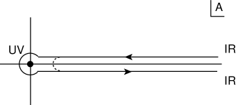
Figure 1: The solid line is the the Saalschutz contour in the complex area ($A$) plane, which is used to continue analytically the prefactor $\Gamma(-s)$ for $s\in Z^{+}$; it has been used in conventional quantum field theory to relate dimensional regularization to the Bogoliubov-Parasiuk-Hepp-Zimmermann renormalization method. The dashed line denotes the regularized contour, which avoids the ultraviolet fixed point $A\rightarrow 0$, which is used in the Closed Time-like Path formalism.

Within this approach, it is not difficult to see that conventional $S$-matrix elements are in general ill-defined in Liouville-string theory, and that scattering must be described by a non-factorizable $/S$-matrix. Decomposing the Liouville field in an orthonormal mode sum: $\phi(z,{\bar{z}})=\sum_{n}c_{n}\phi_{n}=c_{0}\phi_{0}+\sum_{n\neq 0}\phi_{n}$, where $\nabla^{2}\phi_{n}=-\epsilon_{n}\phi_{n}~{}:~{}n=0,1,2,\dots$, and we separate the zero mode $\phi_{0}\propto A^{-\frac{1}{2}}$ with $\epsilon_{0}=0$. The correlation function with $\phi_{0}$ subtracted may be written as

$${\tilde{A}}_{N}\propto \int \Pi_{n\neq 0}dc_{n}exp(-\frac{1}{8\pi}\sum_{n\neq 0}\epsilon_{n}c_{n}^{2}-\frac{Q}{8\pi}\sum_{n\neq 0}R_{n}c_{n}+$$

$$\sum_{n\neq 0}\alpha_{i}\phi_{n}(z_{i})c_{n})(\int d^{2}\xi\sqrt{{\hat{\gamma}}}e^{\alpha\sum_{n\neq 0}\phi_{n}c_{n}})^{s}$$ (6)

with $R_{n}=\int d^{2}\xi R^{(2)}(\xi)\phi_{n}$. We can compute (6) by analytically continuing [16] $s$ to a positive integer $s\rightarrow n^{+}\in{\bf Z}^{+}$. Denoting $f(x,y)\equiv\sum_{n,m~{}\neq 0}\frac{\phi_{n}(x)\phi_{m}(y)}{\epsilon_{n}}$ and integrating over the $c_{n}$, we find

$${\tilde{A}}_{n+N}\propto exp[\frac{1}{2}\sum_{i,j}\alpha_{i}\alpha_{j}f(z_{i},z_{j})+$$

$$\frac{Q^{2}}{128\pi^{2}}\int\int R(x)R(y)f(x,y)-\sum_{i}\frac{Q}{8\pi}\alpha_{i}\int\sqrt{{\hat{\gamma}}}R(x)f(x,z_{i})]$$ (7)

When one makes an infinitesimal Weyl transformation $\gamma(x,y)\rightarrow\gamma(x,y)(1-\sigma(x,y))$, the correlator ${\tilde{A}}_{N}$ transforms as follows [17, 18]:

$$\delta{\tilde{A}}_{N}\propto[\sum_{i}h_{i}\sigma(z_{i})+\frac{Q^{2}}{16\pi}\int d^{2}x\sqrt{{\hat{\gamma}}}{\hat{R}}\sigma(x)+$$ (8)

$$\frac{1}{{\hat{A}}}\{Qs\int d^{2}x\sqrt{{\hat{\gamma}}}\sigma(x)+(s)^{2}\int d^{2}x\sqrt{{\hat{\gamma}}}\sigma(x){\hat{f}}_{R}(x,x)+$$

$$Qs\int\int d^{2}xd^{2}y\sqrt{{\hat{\gamma}}}R(x)\sigma(y){\hat{\cal G}}(x,y)-s\sum_{i}\alpha_{i}\int d^{2}x\sqrt{{\hat{\gamma}}}\sigma(x){\hat{\cal G}}(x,z_{i})-$$

$$\frac{1}{2}s\sum_{i}\alpha_{i}{\hat{f}}_{R}(z_{i},z_{i})\int d^{2}x\sqrt{{\hat{\gamma}}}\sigma(x)-$$

$$\frac{Qs}{16\pi}\int\int d^{2}xd^{2}y\sqrt{{\hat{\gamma}(x)}{\hat{\gamma}}(y)}{\hat{R}}(x){\hat{f}}_{R}(x,x)\sigma(y)\}]{\tilde{A}}_{N}$$

where the hat notation denotes transformed quantities, and ${\cal G}(z,\omega)\equiv f(z,\omega)-\frac{1}{2}(f_{R}(z,z)+f_{R}(\omega,\omega))$: $f_{R}(z,z)={\rm lim}_{\omega\rightarrow z}\left(f(z,\omega)+{\rm ln}d^{2}(z,\omega)\right)$, where $d(z,\omega)$ is the geodesic distance on the world sheet. We see explicitly that (8) contains non-covariant terms $\propto A^{-1}$ if the sum of the anomalous dimensions $s\neq 0$. Thus the generic correlation function $A_{N}$ does not have a well-defined limit as $A\rightarrow 0$.

In [3] we identified the target time as $t=\phi_{0}=-{\rm ln}A$, where $\phi_{0}$ is the world-sheet zero mode of the Liouville field. The normalization follows from a consequence of the canonical form of the kinetic term for the Liouville field $\phi$ in the Liouville $\sigma$ model [6, 3]. The opposite flow of the target time, as compared to that of the Liouville mode, is, on the other hand, a consequence of the ‘bounce’ picture [15, 3] for Liouville flow of Fig. 1. This identification implies that, as a result of the above-mentioned singular behaviour in the ultraviolet limit $A\rightarrow 0$, the correlator ${\tilde{A}}_{N}$ cannot be interpreted as an $S$-matrix element, whenever there is a departure from criticality $s\neq 0$.

When one integrates over the Saalschultz contour in Fig. 1, the integration around the simple pole at $A=0$ yields an imaginary part [15, 3], associated with the instability of the Liouville vacuum. We note, on the other hand, that the integral around the dashed contour shown in Fig. 1, which does not encircle the pole at $A=0$, is well defined. This can be intepreted as a well-defined $/S$-matrix element, which is not, however, factorisable into a product of $S-$ and $S^{\dagger}-$matrix elements, due to the $t$ dependence acquired after the identification $t=-{\rm ln}A$. This formalism is similar to the Closed-Time-Path (CTP) formalism used in non-equilibrium quantum field theories [11], as we now discuss.

In the path-integral formulation of the CTP approach to non-equilibrium field theory [11], the partition function is expressed as an integral over the path of Fig. 2:

$$Z[J_{1},J_{2}:\rho]=\int[D\Phi]<\Phi_{1},t=t_{0}|\rho|\Phi_{2},t=t_{0}>expi\{Tr\Phi D^{-1}\Phi+S_{int}[\Phi]+TrJ.\Phi\}$$ (9)

where $[D\Phi]=[D\Phi_{1}][D\Phi_{2}]$, with $\Phi_{1}(\Phi_{2})$ denoting fields whose time arguments are on the upper (lower) segments of the CTP, with corresponding actions $S_{int}[\Phi_{1,2}]$, $D^{-1}$ is the inverse field propagator and $S_{int}[\Phi]=S_{int}[\Phi_{1}]-S_{int}[\Phi_{2}]$. The density matrix in (9) may be represented as [11]:

$$<\Phi_{1},t_{0}|\rho|\Phi_{2},t_{0}>=exp\{\frac{i}{2}\int K[\Phi_{j}]\}$$ (10)

where the integral extends over space only, at some initial time $t_{0}$, and the kernel $K[\Phi_{i}]$ may in general be expanded in powers of the boundary fields $\Phi_{i}$: $\int K[\Phi_{j}]=const+\int K_{j}\Phi_{j}+\int\frac{1}{2}\Phi_{i}K^{ij}\Phi_{j}+\int\frac{1}{6}K^{ijk}\Phi_{i}\Phi_{j}\Phi_{k}+\dots$.

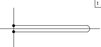
Figure 2: Contour of integration in the complex $t$ plane, used in the Closed Time Path (CTP) formalism. In the Liouville string case $t=-{\rm ln}A$, where $A$ is the world-sheet area.

In our string equivalent of this formalism, the rôle of the action $S_{int}[\Phi_{i}]$ is taken by the Zamolodchikov $C$ function (4), which depends on the $\sigma$-model background couplings/fields $\{g^{i}\}$. The topological summation over genera induces quantum fluctuations in the $\{g^{i}\}$ [19] via a second-quantized effective partition function $Z_{overgenera}=\int[Dg]{\cal P}[g]e^{-C[g]}$: $C[g]=c^{*}-g_{s}^{\chi}\int_{-\infty}^{+\infty}dt{\hat{\beta}}^{i}G_{ij}{\hat{\beta}}^{j}$, where $G_{ij}$ is the Zamolodchikov metric in theory space, which is occupied with a probability distribution ${\cal P}[g]$. An extreme case of a non-trivial topology leading to a divergence is one in which an infinitely long tube joins two distant parts of a Riemann surface. In this case, the string propagator along the tube takes the form

$${\cal D}=\sum_{m}\int_{\delta}\frac{dq}{q}\frac{d{\overline{q}}}{{\overline{q}}}q^{L_{0}}{\overline{q}}^{{\overline{L}}_{0}}|m><m|$$ (11)

which has a double logarithmic divergence as the ‘size’ of the tube $\delta\rightarrow 0$. This scale may be absorbed in a generalized version of the Fischler-Susskind mechanism [20], by introducing quantized couplings, ${\hat{g}}^{i}(t):t=-{\rm ln}\delta$, with a theory-space probability distribution

$${\cal P}[g]=e^{-({\hat{g}}^{i}(t)-g^{*i})G_{ij}({\hat{g}}^{j}(t)-g^{*j})/\Gamma(\delta)}$$ (12)

where $\Gamma(\delta)\propto|{\rm ln}\delta|$ as $\delta\rightarrow 0$ absorbs the infinities associated with the pinched world-sheet tube. The analysis requires the introduction of world-sheet wormhole parameters [21, 19, 22], which parallels the treatment of space-time wormhole parameters in four-dimensional field theories [23]. In our interpretation of the Liouville scale as target time, flowing opposite to the conventional renormalization-group flow [3, 8, 15], the above picture matches the standard renormalization-group approach, when one identifies $t_{\infty}$ with the infrared fixed point. In this way one arrives at a (Liouville) string equivalent of the initial-state density matrix (10).

After these preliminaries, we are now ready to present our construction of $D$-brane foam, as an example of the above formalism. Compared to previous quantum treatments of $D$ branes [9], the key physics step is to find a representation of the appearance and disappearance of virtual $D$ branes. We shall argue that this may be found in the context of the $\sigma$-model description of point defects on the world sheet, namely monopoles and vortices, which are described by the following partition function [24]:

$$Z = \int D{\tilde{X}}exp(-\beta S_{eff}({\tilde{X}}))$$

$$\beta S_{eff} = \int d^{2}z[2\partial{\tilde{X}}{\overline{\partial}}{\tilde{X}}+\frac{1}{4\pi}[\gamma_{v}\omega^{\frac{\alpha}{2}-2}(2\sqrt{|g(z)|})^{1-\frac{\alpha}{4}}:cos(\sqrt{2\pi\sqrt{\beta}q}[{\tilde{X}}(z)+{\tilde{X}}({\bar{z}})]):$$ (13)

$$+ \frac{1}{4\pi}[\gamma_{v}\omega^{\frac{\alpha^{\prime}}{2}-2}(2\sqrt{|g(z)|})^{1-\frac{\alpha^{\prime}}{4}}:cos(\frac{e}{\sqrt{\beta}}[{\tilde{X}}(z)-{\tilde{X}}({\bar{z}})]):]$$

where $\alpha\equiv 2\pi\beta q$,$\alpha^{\prime}\equiv e^{2}/2\pi\beta$: $q$ ($e$) is the vortex (monopole) charge, $\gamma_{v,m}$ are the fugacities for vortices and monopoles, and ${\tilde{X}}$ is a $\sigma$-model field, whose world-sheet equation of motion admits vortex and monopole solutions:

$$\partial_{z}\partial_{\bar{z}}{\tilde{X}}_{v}=i\pi\frac{q}{2}[\delta(z-z_{1})-\delta(z-z_{2})],\qquad\partial_{z}\partial_{\bar{z}}{\tilde{X}}_{m}=-\frac{e\pi}{2}[\delta(z-z_{1})-\delta(z-z_{2})]$$ (14)

We note that $\beta^{-1}$ plays the rôle of an effective temperature in (13), which requires for its specification an ultraviolet (angular) cut-off $\omega$. The vortex and monopole operators have anomalous dimensions:

$$\Delta_{m}=\frac{\alpha}{4}=\frac{\pi\beta}{2}q^{2},\qquad\Delta_{m}=\frac{\alpha^{\prime}}{4}=\frac{e^{2}}{8\pi\beta}$$ (15)

and the system (13) is invariant under the T-duality transformation [24]: $\pi\beta\leftarrow\rightarrow\frac{1}{4\pi\beta}~{};~{}q\leftarrow\rightarrow e$. We identify ${\tilde{X}}$ in (13) with the rescaled Liouville field $\sqrt{\frac{C-25}{3g_{s}^{\chi}}}\phi$, in which classical solutions to the equations of motion and spin-wave fluctuations have been subtracted [24], and relate $\beta$ to the Zamolodchikov $C$ function of the accompanying matter [24]: $\beta\rightarrow\frac{3g_{s}^{\chi}}{\pi(C-25)}$. We will be interested in the case $C>25$, and we shall consider only irrelevant deformations, that do not drive the theory to a new fixed point. The world-sheet system is then in a dipole phase [24]. We note that this system has the general features discussed previously, namely non-conformal deformations, non-trivial Liouville dynamics, and dependence on an ultraviolet cutoff. Furthermore, this system was discussed previously [3] as a model for space time foam in the context of $(1+1)$-dimensional string black holes.

To see why we claim that it can be used to represent $D$-brane foam, we first consider the scattering of close string states $V_{T}(X)=exp(ik_{M}X^{M}-iEX^{0}):M=1,\dots D_{cr}-1$, where $D_{cr}$ is the critical space-time dimension, in the presence of a monopole defect. An essential aspect of this problem is the singular behaviour of the operator product expansion of $V_{T}$ and a monopole operator $V_{m}$. Treating the latter as a sine-Gordon deformation of (13), computing at the tree level using the free world-sheet action, and suppressing for brevity anti-holomorphic parts, we find

$$\hbox{Lim}_{z\rightarrow w}<V_{T}(X^{0},X^{i})(z)V_{m}(X^{0})(w)\dots>$$ (16)

$$\sim\int d^{D}k\int dE\delta^{D}(k)(\dots)[\delta(\Sigma E+\beta)(z-w)^{-\Delta_{T}-\Delta_{m}}+$$

$$\delta(\Sigma E-\beta)(z-w)^{-\Delta_{T}-\Delta_{m}}]$$

where $\Delta_{T}=\frac{E^{2}}{2}$, the energy-conservation $\delta$ functions result from integration over the Liouville field ${\tilde{X}}\equiv X^{0}$, and $(\dots)$ indicates factors related to the spatial momentum components of $V_{T}$, other vertex operators in the correlation function, etc.. We see that (16) has cuts for generic values of $\Delta_{T}+\Delta_{m}$, causing the theory to become that of an open string.

In the particular case of the tree-level three-point correlation function ${\cal A}_{TTm}=<V_{T}(E_{1})V_{T}(E_{2})V_{m}(e/\beta^{1/2})>$, integration over the Liouville field $X^{0}$ imposes energy conservation in the form: ${\cal A}_{TTm}\propto[\delta(E_{1}+E_{2}+e/\sqrt{\beta}){\cal A}_{1}^{\prime}+\delta(E_{1}+E_{2}-e/\sqrt{\beta}){\cal A}_{2}^{\prime}]$ where the two terms arise from the cosine form of the monopole vertex operator (13), though only the second term is in the physical region $E_{1,2}>0$:

$$E_{1}+E_{2}=e/\sqrt{\beta}=e\left(\pi(C-25)/3g_{s}^{\chi}\right)^{\frac{1}{2}}$$ (17)

This equation is consistent with the monopole describing a massive particle in target space-time if $C>25$. For this, we consider a model with 25 additional space-like coordinates $X^{i}$ coupled to a linear dilaton background [6]: $\int d^{2}z\partial X^{i}\partial X^{j}\delta_{ij}+i\int d^{2}zQ\eta_{i}X^{i}R^{(2)}$, where $\eta_{i}$ a fixed vector, which has $C=26+{\cal O}(\beta^{i})^{2}$ if $Q=\sqrt{{C-25\over 3}}$.

In the open string picture (16), induced by the interaction of matter with the defects, one may assume that the world-sheet curvature $R^{(2)}$ is concentrated along the cut, in which case the linear-dilaton background term contributes an extrinsic-curvature term ${\hat{k}}$ on the world-sheet boundary

$$i\int_{\partial\Sigma}Q\eta_{i}X^{i}{\hat{k}}$$ (18)

Since we wish to study the effects of virtual $D$ branes, we need to be able to sew tree-level amplitudes into loop diagrams with internal monopoles. This requires a better understanding of the appropriate boundary conditions along the cut in the world sheet. In the case of the Liouville field $\phi=X^{0}$, the appropriate boundary condition in open string theory has been derived in [25]:

$$\partial_{n}X^{0}+i\frac{{\hat{k}}}{2}Q=0$$ (19)

where ${\hat{k}}$ is the extrinsic curvature of the fiducial metric, up to a possible cosmological constant term and higher-order quantum corrections. We note that (19) reduces to Neumann boundary conditions in the critical limit $Q\rightarrow 0$, as is the case in the simplified situation considered here and in ref. [24], where the cosmological constant term is ignored in the Liouville action, thereby allowing the decoupling of the spin-wave part from the monopole field ${\tilde{X}}\equiv X^{0}$. The space coordinates $X^{i}$ may be taken to have either Neumann or Dirichlet boundary conditions, which are related by a T-duality transformation. If Neumann boundary conditions are chosen, one must introduce a background gauge field $A_{i}$ related to possible Chan-Paton factors at the ends of the open string, and the corresponding $\sigma$-model path integral is:

$$Z=\int DX^{i}DX^{0}e^{-\int_{\Sigma}d^{2}z\frac{1}{4\pi\alpha^{\prime}}[\partial X^{i}{\overline{\partial}}X^{i}\delta_{ij}-\partial X^{0}{\overline{\partial}}X^{0}]-i\int_{\partial\Sigma}A_{i}(X^{0})\partial_{\tau}X^{i}+i\int_{\partial\Sigma}{\hat{k}}Q\eta_{i}X^{i}}$$ (20)

where $\partial_{\tau}$ denotes a tangential derivative on the world-sheet boundary $\partial\Sigma$. The Abelian background gauge field depends on time $X^{0}$ only, and we work in the gauge $A_{0}=0$ for simplicity.

It is convenient for our purposes to make a $T$-duality transformation: $Y_{\alpha}^{i}=\partial_{\alpha}X^{i}$: $\epsilon_{\alpha\beta}\partial_{\alpha}Y_{\beta}^{i}=0$, which yields a tractable weak-coupling formalism. This we implement in (20) using Lagrange multipliers $\lambda_{\alpha}^{i},{\widehat{X}}^{i}$ [26]:

$$Z=\int D{\widehat{X}}^{i}\int DX^{i}DY^{i}_{\alpha}\delta(Y^{i}_{\alpha}-\partial_{\alpha}X^{i})e^{-\int_{\Sigma}d^{2}z[(Y_{\alpha}^{i})^{2}-\partial X^{0}{\overline{\partial}}X^{0}]-i\int_{\partial\Sigma}A_{i}(X^{0})Y_{\tau}^{i}}$$ (21)

$$e^{-i\int_{\Sigma}d^{2}z{\widehat{X}}^{i}\epsilon_{\alpha\beta}\partial_{\beta}Y^{\alpha}_{i}-i\int_{\partial\Sigma}{\hat{k}}Q\eta_{i}X^{i}}=$$

$$\int D{\widehat{X}}^{i}\int D\lambda_{\tau}^{i}\int DX^{i}DY^{\alpha}_{i}e^{-\int_{\Sigma}d^{2}z[(Y_{\alpha}^{i})^{2}-\partial X^{0}{\overline{\partial}}X^{0}]-i\int_{\partial\Sigma}A_{i}(X^{0})Y_{\tau}^{i}-i\int_{\partial\Sigma}Y_{\tau}^{i}{\widehat{X}}^{i}}$$

$$e^{i\int_{\Sigma}d^{2}zY_{\alpha}^{i}\epsilon_{\alpha\beta}\partial_{\beta}{\widehat{X}}^{i}-i\int_{\partial\Sigma}(Y_{\tau}^{i}\lambda_{\tau}^{i}+X^{i}\partial_{\tau}\lambda_{\tau}^{i}+{\hat{k}}Q\eta_{i}X^{i})}$$

The boundary term in the integration over $Y_{\tau}^{i}$ results in the Dirichlet constraints:

$${\widehat{X}}^{i}+\lambda_{\tau}^{i}+A^{i}(X^{0})=0,~{}~{}\partial_{\tau}\lambda_{\tau}^{i}+i{\hat{k}}Q\eta^{i}=0\qquad{\rm on~{}\partial\Sigma}$$ (22)

with ${\widehat{X}}^{i}$ described by a free $\sigma$-model action in the bulk . The boundary condition (22) is not conformally invariant, which is known to be the case for fixed Dirichlet boundary conditions in the presence of a linear-dilaton background [9]. This ‘conformal anomaly’ in the dual theory keeps track of the fact that the matter system has central charge 26, but a non-critical number ($D=25$) of spatial dimensions [6].

Conformal invariance can be restored by Liouville dressing . Fixed Dirichlet boundary conditions are obtained by shifting the $X^{0}$ field in such a way so that $A_{i}(X^{0})+\lambda_{\tau}^{i}=A_{i}^{\prime}(X^{{}^{\prime}0})$, which can be done with an appropriate choice of $A(X^{0})$ (‘Liouville dressing’). The simplest choice is a gauge potential corresponding to a constant ‘electric’ field $v_{i}$:

$$A_{i}(X^{0})={\rm const}+v_{i}X^{0}$$ (23)

where $v_{i}$ is determined from (22), and is found to be proportional to $\eta_{i}{\hat{k}}Q$. Physically, this means that a non-critical-dimension matter string theory, in a linear-dilaton background [6], corresponds, upon $T$-dualization in our Liouville framework, to a moving $D$-brane with a velocity $v_{i}$ determined by the matter central charge deficit $Q$. The ‘motion’ of the $D$-brane implies target-time dependence provided by the Liouville field [3].

We note that, by applying the above dualization procedure for $p$ of the spatial coordinates, one can generate generic $p$-brane configurations, with $p\geq 1$ Dirichlet directions. The $D0$ particle is the first non-trivial structure in this hierarchy of stringy structures. Since the collective coordinates of such $D0$ branes are associated with a canonically-quantized phase space [22, 19], the above construction may be thought of as providing for the emergence of a target space-time from string solitonic structures, where the space is provided by the collective coordinates describing the position of the string soliton, and the time is given by the Liouville mode of the non-critical two-dimensional model describing the interaction of string matter with the world-sheet defects.

From the point of view of the target-space wave function of the string, the above background gauge fields appear as Bohm-Aharonov phase factors. To see this, suppose that a closed-string state encounters a monopole defect on the world sheet at $(\sigma_{0},\tau_{0})$, corresponding to a spatial location $y^{i}$ and a time $X^{0}=\tau_{0}$ in the light-cone gauge. The gauge field was absent before this encounter, so has a step-function singularity:

$$A(X^{0})^{i}=(y^{i}-(X^{0}-\tau_{0})F^{0i})\Theta(X^{0}-\tau_{0})$$ (24)

where $F^{0i}$ is the electric field strength, which has a $\delta(X^{0}-\tau_{0})$ singularity, but is otherwise conformally invariant. In the T-dual picture, there is a corresponding ‘sudden’ appearance of Dirichlet boundary conditions, breaking conformal invariance, that we interpret as the excitation of a $D$ brane in the vacuum. There is a corresponding singularity in the space-time curvature [10] associated with the creation of the world-sheet monopole:

$$R~{}\ni~{}-2\frac{25\delta(X^{0}-\tau_{0})}{[1+\Theta(X^{0}-\tau_{0})(\sum_{i=1}^{25}y_{i}^{2})]^{2}}$$ (25)

which confirms our interpretation that the appearance of the world-sheet monopole corresponds to the appearance of a black hole represented by a $D$ brane.

Propagation of a light closed-string particle through this representation of $D$-brane foam involves, at the lowest order, a diagram with a disk topology, internal tachyon vertices, and the boundary conditions (19, 22). This may describe scattering through a real (or virtual) $D$-brane state, with production and decay amplitudes $A_{TTm}$, subject to the energy-conservation condition (17). The next term in a topological expansion in genus $g=2-2\#_{handles}-\#_{holes}$ is an annulus with closed-string operator insertions. As has been discussed elsewhere [28], this has a singularity ${\cal A}\sim\delta(E_{1}+E_{2})\sqrt{\frac{1}{{\rm ln}(\delta)}}$ in the pinched annulus configuration $\delta\rightarrow 0$, which is regularized by introducing recoil operators [19, 29, 10] $C,D$ to describe the back reaction of the struck $D$ brane:

$$V_{rec}=y_{i}C+u_{i}D\qquad:C\equiv\epsilon\int_{\partial\Sigma}\Theta_{\epsilon}(X^{0})\partial_{n}X^{i}\qquad D\equiv\int_{\partial\Sigma}X^{0}\Theta_{\epsilon}(X^{0})\partial_{n}X^{i}$$ (26)

where ${\rm lim}_{\epsilon\rightarrow 0}\Theta_{\epsilon}(X^{0})$ is a suitable integral representation of the step function, and $y_{i}$, $u_{i}$ are the position and momentum of the recoiling $D$ brane. As discussed in [10], we identify $1/\epsilon^{2}\sim\hbox{ln}\delta$, and in turn, using the Fischler-Susskind mechanism [20] on the world sheet to relate renormalization-group infinities among different genus surfaces, we identify $t\sim{\rm ln}\delta$. The operators $C,D$ consitute a logarithmic pair [29] with $<C(z)C(0)>$, $<C(z)D(0)>$ non-singular as $\epsilon\rightarrow 0^{+}$, whereas $<D(z)D(0)>$ is singular with a world-sheet scale dependence [29] $D\rightarrow D+tC$, from which we infer that $u_{i}\rightarrow u_{i}$, $y_{i}\rightarrow y_{i}+u_{i}t$, corresponding to a Galilean time transformation [22], as is appropriate for a heavy $D$ brane with mass $\propto 1/g_{s}$ (28).

The logarithmic operators (26) make divergent contributions to the genus-0 amplitude in the limit where it becomes a pair of Riemann surfaces $\Sigma_{1},\Sigma_{2}$ connected by a degenerate strip [19, 22]:

$${\cal A}_{strip}\sim g_{s} ({\rm ln}^{2}\delta)\int d^{2}z_{1}D(z_{1})\int d^{2}z_{2}C(z_{2}),$$ (27)

$$g_{s} {\rm ln}\delta\int d^{2}z_{1}D(z_{1})\int d^{2}z_{2}D(z_{2}),\quad g_{s}{\rm ln}\delta\int d^{2}z_{1}C(z_{1})\int d^{2}z_{2}C(z_{2})$$

Assuming a dilute gas of monopole defects on the world sheet, the amplitudes (27) become contributions to the effective action [19, 22]. One may then seek to cancel them or else to absorb them into scale-dependent $\sigma$-model couplings as described in equations (11, 12). If they could all be cancelled, the corresponding $\sigma$-model would be conformally invariant, whereas absorption of these divergent contributions would result in departures from criticality.

The leading double logarithm associated with the CD combination in (27) may indeed be cancelled [22] by imposing the momentum conservation condition

$$u_{i}=g_{s}(k_{1}+k_{2})_{i}$$ (28)

as expected for a $D$ brane soliton of mass $1/g_{s}$, which is also consistent with the tree-level energy-conservation condition in (17), obtained by integration over the Liouville zero mode. From the point of view of the Liouville theory on the open world sheet (21, 22), the tree-level monopole mass term arises from a boundary term $i\int_{\partial\Sigma}QX^{0}{\hat{k}}$ in the effective action [25], where ${\hat{k}}$ is the extrinsic curvature and $Q$ is given by equation (3). When the Liouville integration is performed at the quantum level, $Q$ is replaced by its value in (3), which receives a contribution from $\beta_{y_{i}}=u_{i}$ [10], by virtue of the logarithmic operator product expansion of $C$ and $D$ [29]. Expanding the right-hand-side of (3), using (4), for small $|u_{i}u^{i}|<<1$, we find the quantum energy conservation condition:

$$E_{1}+E_{2}=\frac{e}{\sqrt{\beta}}=e\left(\pi(C-25)/3g_{s}\right)^{1/2}=\frac{e}{\sqrt{g_{s}}}(1+\frac{u_{i}^{2}}{2}+\dots)$$ (29)

The result (29) matches the momentum conservation condition (28) upon setting $e\sqrt{\pi/3}=1/\sqrt{g_{s}}$, thereby confirming our interpretation of time as the Liouville field [3, 8]. Thus, cancellation of the leading double logarithm in (27) enforces energy conservation $\frac{d}{dt}<E>=0$, as argued previously [3] in a general renormalization-group approach to Liouville dynamics.

The single logarithms associated with the CC and DD contributions in (27) are a different story, since they can only be absorbed into quantum coupling parameters [19, 22]: ${\hat{y}_{i}}=y_{i}+\alpha_{C}\sqrt{{\rm ln}\delta},{\hat{u}}_{i}=u_{i}+\alpha_{D}\sqrt{{\rm ln}\delta}$. The resulting probability distribution in theory space (12) becomes time dependent [19, 22]:

$${\cal P}\sim\frac{1}{g_{s}^{2}ln\delta}e^{-\frac{({\hat{q}}_{m}-q_{m})G^{mn}({\hat{q}}_{n}-q_{n})}{g_{s}^{2}ln\delta}}$$ (30)

where $q_{m}\equiv\{y_{i},u_{i}\}$. Within the CTP-like interpretation of the Saalschutz contour reviewed earlier, this corresponds to a time-dependent $/S$-matrix transition from the initial-state density matrix.

Although this is compatible with energy conservation in the mean, as discussed previously, it entails a non-quantum-mechanical modification of the energy fluctuations $(E-<E>)^{2}$. It has been shown elsewhere [3] that these may be related to the non-zero renormalization group functions $\beta_{i}$:

$$\frac{d}{dt}<(E-<E>)^{2}>=<(\frac{d}{dt}\beta^{i})G_{ij}\beta^{j}>$$ (31)

It has been shown [19] in the Liouville-string framework that $\frac{d}{dt}G_{ij}=QG_{ij}$. Thus, using the result [3] that ${\dot{S}}=\beta^{i}G_{ij}\beta^{j}$, we find

$$\frac{d}{dt}<(E-<E>)^{2}>=\frac{1}{2}{\ddot{S}}-Q{\dot{S}}$$ (32)

which may be considered as a quantum-gravitational version of the fluctuation-dissipation theorem of statistical mechanics [3, 19]. We see that, the closer the system lies to its infrared fixed point as $t\rightarrow\infty$, the more classical it becomes, in the sense of an increase in entropy and a corresponding decrease in its energy fluctuations. This result in the context of Liouville $D$ branes is in agreement with the general picture, advocated in [3], that a classical field-theoretic vacuum is obtained from a non-critical string theory via decoherence in ‘theory space’.

To acquire some feeling for the possible order of magnitude of such decohering effects, we estimate from (28) that $|\beta_{y_{i}}|=|u_{i}|={\cal O}(E/M_{P})$, where $E$ is the typical energy of a closed-string light-particle state, and we neglect numerical factors, powers of $g_{s}$, etc. Correspondingly, assuming an effective $D$-brane density of order unity per Planck volume, we estimate ${\dot{S}}={\cal O}(E^{2}/M_{P}^{2})$, whereas $\frac{d}{dt}<(E-<E>)^{2}>$ vanishes to this order, since our heavy branes do not accelerate: $\frac{d}{dt}u_{i}=0$ [10, 22]. As has been discussed elsewhere [3], the corresponding time-evolution equation for the density matrix $\rho$ of a light-particle state takes the form:

$$\frac{\partial}{\partial t}\rho=i[H,\rho]+/\delta H\rho:~{}~{}/\delta H=i\beta^{i}G_{ij}[g^{j},~{}]$$ (33)

and we estimate $|/\delta H|={\cal O}(E^{2}/M_{P})$, in agreement with previous estimates [3, 30], and close in order of magnitude to the experimental bound from the $K^{0}-{\overline{K}}^{0}$ system [2, 31]. In higher orders, we expect $\frac{d}{dt}\beta^{i}=\beta^{m}\partial_{m}\beta^{i}\sim 2\beta^{m}~{}(c^{i}_{mk}g^{k}+{\cal O}[g^{2}])$, where the operator-product-expansion coefficients $c^{i}_{jk}$ are of order $E^{2}/M_{P}^{2}$ in the closed-string sector, or $E/M_{P}$ in the open-string sector, as in the case of $D$ branes. Thus, (31) is suppressed - as compared to ${/\delta H}$ (33) - by higher powers of Planck Mass, at least as $E^{3}/M_{P}^{2}$ in the open-string sector, which makes such energy fluctuations difficult to detect in foreseeable experimental facilitites.

Finally, we comment on the new uncertainty relations that stem from the above construction, which could be used to probe the quantum-gravity structure of a $D$-brane space time. The key observation is that the target time $X^{0}\propto\sqrt{C-25}\varphi$, where $\varphi$ is the original Liouville field appearing in the conformal scale factor of the world-sheet metric. From (3), then, and the fact that summing over world-sheet genera leads to a canonical quantization of the $\sigma$-model couplings $y_{i},u_{i}$ [19, 22], we see that in this picture $X^{0}$ appears as an ‘operator’ in the $D$-brane collective phase space, leading to non-trivial commutation relations between the time $X^{0}$ and the position (collective) coordinates of the $D$ brane [32]. It can be easily seen that, for slowly-moving non-relativistic branes: $|u_{i}|^{2}<<1$ as we are considering here, such commutators lead to the following space-time uncertainty relation:

$$\Delta y_{i}\Delta X^{0}\geq g_{s}^{1/2}u_{i}+\dots$$ (34)

Non-trivial space time uncertainty relations of the form (34), but independent of the string coupling, had been derived previously in the context of critical (conformal) strings and $D$ branes in ref. [33].

References

- [1] S. Hawking, Comm. Math. Phys. 87 (1982), 395.
- [2] J. Ellis, J. Hagelin, D.V. Nanopoulos, and M. Srednicki, Nucl. Phys. B241 (1984), 381.
- [3] J. Ellis, N.E. Mavromatos and D.V. Nanopoulos, Lectures presented at the Erice Summer School 1993; Published in Erice Subnuclear Series (World Sci.) Vol. 31 (1993), 1, hep-th/9403133.
- [4] E. Witten, Phys. Rev. D44 (1991), 344.
- [5] J. Ellis, N.E. Mavromatos and D.V. Nanopoulos, Phys. Lett. B272 (1991), 56.
- [6] I. Antoniadis, C. Bachas, J. Ellis, and D.V. Nanopoulos, Phys. Lett. B211 (1988), 393; Nucl. Phys. B328 (1989), 117.
- [7] F. David, Mod. Phys. Lett. A3 (1988), 1651; J. Distler and H. Kawai, Nucl. Phys. B321 (1989), 509.
- [8] I. Kogan, preprint UBCTP-91-13 (1991); Proc. Particles and Fields 91, p. 837, Vancouver 18-21 April 1991 (eds. D. Axen, D. Bryman and M. Comyn, World Sci. 1992).
- [9] J. Dai, R.G. Leigh and J. Polchinski, Mod. Phys. Lett. A4 (1989), 2073; J. Polchinski, Phys. Rev. D50 (1994), 6041 ; Phys. Rev. Lett. 75 (1995) 184; C. Bachas, Phys. Lett. B374 (1996), 37; J. Polchinski, S. Chaudhuri and C. Johnson, NSF-ITP-96-003 preprint, hep-th/9602052, and references therein; J. Polchinski, NSF-ITP-96-145, hepth/9611050, and references therein.
- [10] J. Ellis, N.E. Mavromatos and D.V. Nanopoulos, preprint CERN-TH/96-264, OUTP-57-P, hep-th/9609238.
-
[11]
The CTP formalism may be attributed to:
J. Schwinger, J. Math. Phys. 2 (1961), 407. For recent reviews, whose formalism we follow here, see: E. Calzetta and B.L. Hu, Phys. Rev. D37 (1988), 2878; E. Calzetta, S. Habib and B.L. Hu, Phys. Rev. D37 (1988), 2901. - [12] I. Klebanov, I. Kogan and A.M. Polyakov, Phys. Rev. Lett. 71 (1993), 3243; C. Schmidhuber, Nucl. Phys. B404 (1993), 342.
- [13] A.B. Zamolodchikov, JETP Lett. 43 (1986), 730; Sov. J. Nucl. Phys. 46 (1987), 1090.
- [14] J. Ellis, N.E. Mavromatos and D.V. Nanopoulos, CERN, ENS-LAPP and Texas A & M Univ. preprint, CERN-TH.6897/93, ENS-LAPP-A427-93, CTP-TAMU-30/93; ACT-10/93 (1993); hep-th/9305117.
- [15] I. Kogan, Phys. Lett. B265 (1991), 269.
- [16] M. Goulian and M. Li, Phys. Rev. Lett. 66 (1991), 345.
- [17] N.E. Mavromatos and D.V. Nanopoulos, Int. J. Mod. Phys. B11 (1997), 851.
- [18] L. Alvarez-Gaumé, unpublished notes on Two-Dimensional Gravity and Liouville Theory (1991).
- [19] J. Ellis, N.E. Mavromatos and D.V. Nanopoulos, Mod. Phys. Lett. A10 (1995), 1685; preprint ACT-04/96, CERN-TH/96-81, CTP-TAMU-11/96, OUTP-96-15P; hep-th/9605046, Int. J. Mod. Phys. A, in press.
- [20] W. Fischler and L. Susskind, Phys. Lett. B171 (1986), 383; ibid. 173 (1986), 262.
- [21] W. Fischler, S. Paban and M. Rozali, Phys. Lett. B352 (1995), 298; Phys. Lett. B381 (1996), 62; D. Berenstein, R. Corrado, W. Fischler, S. Paban and M. Rozali, Phys. Lett. B384 (1996), 93.
- [22] F. Lizzi and N.E. Mavromatos, OUTP-96-66P preprint (1996), hep-th/9611040, Phys. Rev. D in press.
- [23] S. Coleman, Nucl. Phys. B310 (1988), 643; T. Banks, I. Klebanov and L. Susskind, Nucl. Phys. B (1988), .
- [24] B. Ovrut and S. Thomas, Phys. Lett. B257 (1991), 292.
- [25] J. Ambjorn, K. Hasayaka and R. Nakayama, hep-th/9702019.
- [26] H. Dorn and H-J. Otto, Phys. Lett. B381 (1996); hep-th/9702018; J. Borlaf and Y. Lozano, hep-th/9607051.
- [27] M. Li, Phys. Rev. D54 (1996), 1644.
- [28] V. Periwal and O. Tafjord, Phys. Rev. D54 (1996), 3690.
- [29] I. Kogan, N. E. Mavromatos and J.F. Wheater, Phys. Lett. B387 (1996), 483.
- [30] J. Ellis, N.E. Mavromatos, D.V. Nanopoulos and E. Winstanley, Mod. Phys. Lett. A12 (1997), 243.
- [31] CPLEAR Collaboration and J. Ellis, J. Lopez, N.E. Mavromatos and D.V. Nanopoulos, Phys. Lett. B364 (1995), 239.
- [32] G. Amelino-Camelia, J. Ellis, N.E. Mavromatos and D.V. Nanopoulos, hep-th/9701144.
- [33] T. Yoneya, Mod. Phys. Lett. A4 (1989), 1587; M. Li and T. Yoneya, Phys. Rev. Lett. 78 (1997), 1219.