DAMTP 97-33. hep-th/9704153.
SU(3) monopoles and their fields.

Abstract

Some aspects of the fields of charge two SU(3) monopoles with minimal symmetry breaking are discussed. A certain class of solutions look like SU(2) monopoles embedded in SU(3) with a transition region or “cloud” surrounding the monopoles. For large cloud size the relative moduli space metric splits as a direct product ${\cal AH}\times\hbox{\upright\hbox to0.0pt{I\hss}\kern 1.7ptR}^{4}$ where ${\cal AH}$ is the Atiyah-Hitchin metric for SU(2) monopoles and $\hbox{\upright\hbox to0.0pt{I\hss}\kern 1.7ptR}^{4}$ has the flat metric. Thus the cloud is parametrised by $\hbox{\upright\hbox to0.0pt{I\hss}\kern 1.7ptR}^{4}$ which corresponds to its radius and SO(3) orientation. We solve for the long-range fields in this region, and examine the energy density and rotational moments of inertia. The moduli space metric for these monopoles, given by Dancer, is also expressed in a more explicit form.

1 Introduction

In this paper we examine some aspects of charge two BPS monopoles in a gauge theory SU(3) spontaneously broken by an adjoint Higgs to U(2). Their moduli space was found by Dancer in [1], and subsequently studied in [2, 3, 4]. Magnetic monopoles in SU(2) gauge theory have been the focus of considerable interest. Recently, there has been renewed interest in monopoles of higher rank gauge groups mainly in relation to electric-magnetic duality [5, 6, 7, 8, 9]. Substantial progress has been made in theories where the gauge symmetry is broken to the maximal torus. However if the unbroken symmetry group contains a non-Abelian component various complications arise and much less is known. For SU(3) monopoles with minimal symmetry breaking the topological charge is specified by a single integer $k$. But as pointed out in [10] there is a further gauge invariant classification of monopoles, with the result that the charge $k$ moduli space is stratified into different connected components. Charge one monopoles are given by embeddings of the charge one SU(2) monopole. Their moduli space is given by $\hbox{\upright\hbox to0.0pt{I\hss}\kern 1.7ptR}^{3}\times S^{3}$, which is fibred over $S^{2}$ with fibre $\hbox{\upright\hbox to0.0pt{I\hss}\kern 1.7ptR}^{3}\times U(1)$. Points in $S^{2}$ label different possible embeddings of the SU(2) solution, however it is well known that it is not possible to move along the $S^{2}$ factor [11, 12, 13] due to the non-Abelian nature of the long-range fields (the long-range magnetic field does not commute with all the generators of the unbroken gauge group).

Charge two monopoles appear in two distinct categories depending on whether or not the long-range fields are Abelian. Monopoles with non-Abelian long-range magnetic fields are given by embeddings of charge two SU(2) solutions, the moduli space is of dimension ten (which is fibred over $S^{2}$ with fibre the charge two SU(2) moduli space). However if the long-range magnetic fields are Abelian the moduli space is more complicated and has dimension twelve. This phenomenon where the charge $k$ moduli space is stratified, with different components having different dimensions occurs for any gauge theory in which the unbroken subgroup is non-Abelian [14, 15].

In the presence of a monopole whose long-range fields are non-Abelian it is not possible in general to define a global color gauge transform which is orthogonal to the orbits of gauge transforms which are 1 at spatial infinity (i.e. little gauge transforms) [11]. As Abouelsaood showed in [12], this is a consequence of the result [13], which showed the impossibility of globally defining (in any regular gauge) a full set of generators that commute with the Higgs field on a two sphere at infinity when the monopole has long-range non-Abelian fields. In the SU(3) theory this is so for embedded SU(2) monopoles. However, when the long-range fields are Abelian such transformations are possible and the moduli space gains a normalisable action of SU(2). This suggests that the moduli space for the larger strata would be of dimension eleven rather than eight as for embedded SU(2) monopoles (ignoring the $S^{2}$ fibre). However, it is known that the moduli space is of dimension twelve [14, 16], and so an extra parameter appears whose physical interpretation is somewhat unclear. We shall see that in certain regions the monopoles look like embedded SU(2) monopoles surrounded by a non-Abelian cloud whose approximate radius can be attributed to this extra parameter.

It has been proved that the moduli space of monopoles for many gauge groups is in 1-1 correspondence with the moduli space of solutions to Nahm’s equations on a given interval with certain boundary conditions [17]. This correspondence is known to be an isometry for SU(2) monopoles and SU(n+1) monopoles broken to U(n), which includes the present case [18, 19]. In [1], Dancer has constructed the metric on the moduli space of solutions to Nahm’s equations which is a twelve dimensional hyperkähler manifold with free, isometric actions of $R^{3}$, U(2), and Spin(3). By [19] this gives the metric on the two monopole moduli space.

The Dancer manifold can be thought of as having a boundary which corresponds to the space of embedded SU(2) monopoles (however the manifold with the induced $L^{2}$ metric is complete and the boundary is infinitely far away in metric distance). Like in the SU(2) case, the monopoles have a well-defined center of mass and total U(1) phase. In [1] an implicit expression was given for the relative moduli space metric which has isometry group SO(3)$\times$SO(3). Below, this metric is expressed in terms of invariant one-forms corresponding to the actions of each of the SO(3)’s and two other parameters which roughly measure the monopoles’ separation and how “close” the monopole configuration is to an embedded SU(2) monopole configuration. The expressions for the metric are very complicated and are relegated to the Appendix. However for regions of the moduli space which approach the boundary the metric simplifies into a direct product of ${\cal AH}\times\hbox{\upright\hbox to0.0pt{I\hss}\kern 1.7ptR}^{4}$. An interpretation is that the configuration looks like an embedded charge two SU(2) monopole surrounded by a “cloud” [6], which is parametrised by its physical radius (which is related to the inverse of the coordinate distance from the boundary of the Dancer manifold) and its SO(3) orientation (residual gauge group action). Evidence for this is given by solving for the long-range Higgs and gauge fields in this region of the moduli space. Here, the long-range fields do indeed have this cloud where the fields change from those of a non-Abelian embedded SU(2) monopole to the Abelian fall-off of these monopoles. The long-range fields are obtained from a spherical symmetry ansatz and so our results are only valid at a distance much larger than the separation of the two monopoles. The kinetic energy obtained by varying the size of the cloud may be calculated and is shown to agree with the kinetic energy deduced from the metric. The moments of inertia, corresponding to the SO(3) gauge action, can be read off from the metric and they diverge as the cloud spreads out to infinity.

The presence of the cloud can alter the possible types of monopole scattering from the SU(2) case. For SU(2) monopoles if two monopoles collide head on, they form a torus and then scatter at right angles. Here a different outcome is possible [3]. Incoming monopoles can collide, forming instantaneously a spherically symmetric monopole, but now instead of scattering outwards they continue to approach the embedded SU(2) torus. Due to the conservation of kinetic energy of the incoming monopoles (and angular momentum conservation) the SU(2) monopoles must scatter but in the SU(3) case the kinetic energy is carried off by the cloud while the monopoles’ core is static in the limit of large time.

An alternative description of this cloud was given by Lee, Weinberg and Yi [6]. They proposed that the moduli space of monopoles whose magnetic charge is Abelian can be obtained as a limit of a monopole moduli space in a theory where the gauge group is broken to its maximal torus. Our case, where SU(3) is broken to U(2), can be viewed as a limit of SU(3) broken to U(1)$\times$U(1) as the Higgs expectation value is varied. Then the Dancer moduli space would arise from a space of three monopoles : two of the same type, and the third distinct and becoming massless in the limit. As this monopole becomes massless its core radius expands and eventually loses its identity as a monopole and is manifested as a cloud surrounding the remaining two monopoles.

Section 2 is a review of SU(3) monopoles. For completeness we discuss both cases, SU(3) broken to U(1)$\times$U(1) and SU(3) broken to U(2). In section 3 we consider the charge two monopoles where SU(3) is broken to U(2). In particular we solve for the long-range gauge and Higgs fields in regions of the moduli space which are close to the boundary of embedded SU(2) monopoles. In the Appendix the metric given in [1] is reexpressed in an explicit form.

2 Review of SU(3) Monopoles

We assume throughout that the Higgs field is in the adjoint representation and we are in the BPS limit in which the scalar potential is zero but a nonzero Higgs expectation value is imposed at spatial infinity as a boundary condition. An SU(3) gauge theory can be broken by an adjoint Higgs mechanism to either U(1)$\times$U(1) or U(2). Monopole solutions will occur in either theory. The generators of SU(3) may be chosen to be two commuting operators $H_{1}$, $H_{2}$, together with ladder operators, associated with the roots $\pm\mbox{\boldmath$\alpha$}$, $\pm\mbox{\boldmath$\beta$}$, $\pm(\mbox{\boldmath$\alpha$}+\mbox{\boldmath$\beta$})$ (see figure 1), that obey

$$[H_{i},E_{\mbox{\boldmath$\gamma$}}]=\gamma^{i}E_{\mbox{\boldmath$\gamma$}},\;\;\;\;\;[E_{\mbox{\boldmath$\gamma$}},E_{-\mbox{\boldmath$\gamma$}}]=\gamma^{i}H_{i}\;,$$ (2.1)

for $\gamma$ any root. Following [16] we let $\Phi_{\infty}$ be the asymptotic value of the Higgs field along the positive $x^{3}$-axis. Choose this to lie in the Cartan subalgebra and this defines a vector $\bf{h}$ by $\Phi_{\infty}=\bf{h}.\bf{H}$. If SU(3) is broken to U(1)$\times$U(1), all roots have nonzero inner product with $\bf{h}$ and there is a unique set of simple roots with positive inner product with $\bf{h}$. If SU(3) is broken to U(2) then one of the roots, say $\beta$, is perpendicular to $\bf{h}$. Now there are two choices of simple roots with non-negative inner product with $\bf{h}$; namely $(\mbox{\boldmath$\alpha$},\mbox{\boldmath$\beta$})$ and $(\mbox{\boldmath$\alpha$}+\mbox{\boldmath$\beta$},-\mbox{\boldmath$\beta$})$. Figure 1 illustrates the two different types of symmetry breaking.

Figure 1: (a) SU(3)$\rightarrow U(1)\times U(1)\;\;\;\;$(b) SU(3)$\rightarrow$ U(2)

For any finite energy solution, asymptotically

$$B_{i}=\frac{r_{i}}{4\pi r^{3}}G(\Omega)$$ (2.2)

$G(\Omega)$ is a covariantly constant element of the Lie algebra of SU(3), and takes the value $G_{0}$ along the positive $x^{3}$-axis. The Cartan subalgebra may be chosen so that $G_{0}=\bf{g}.\bf{H}$. The quantisation of magnetic charge [10, 20], ensures that $\bf{g}$ is of the form

$${\bf{g}}=\frac{4\pi}{e}\left\{n\mbox{\boldmath$\alpha$}^{*}+m\mbox{\boldmath$\beta$}^{*}\right\}\;,\;\;\;\;\;\;\mbox{\boldmath$\alpha$}^{*}=\frac{\mbox{\boldmath$\alpha$}}{\mbox{\boldmath$\alpha$}\cdot\mbox{\boldmath$\alpha$}}$$ (2.3)

where $e$ is the gauge coupling, and $n$, $m$ are non-negative integers. We denote such a charge by $(n,m)$.

When SU(3) is broken to U(1)$\times$U(1) the topological charges of the monopoles are determined by a pair of integers, ie. the monopoles can be charged with respect to either of the unbroken U(1)’s. All BPS monopoles may be thought of as superpositions of two fundamental monopoles given by embeddings of the charge one SU(2) monopole [16]. To embed an SU(2) solution note that any root $\gamma$ defines an SU(2) subalgebra by

$$t^{1}(\mbox{\boldmath$\gamma$}) = (2{\mbox{\boldmath$\gamma$}\cdot\mbox{\boldmath$\gamma$}})^{-1/2}(E_{\mbox{\boldmath$\gamma$}}+E_{-\mbox{\boldmath$\gamma$}})$$ (2.4)

$$t^{2}(\mbox{\boldmath$\gamma$}) = -i(2{\mbox{\boldmath$\gamma$}\cdot\mbox{\boldmath$\gamma$}})^{-1/2}(E_{\mbox{\boldmath$\gamma$}}-E_{-\mbox{\boldmath$\gamma$}})$$

$$t^{3}(\mbox{\boldmath$\gamma$}) = \mbox{\boldmath$\gamma$}^{*}\cdot{\bf{H}}\;.$$

If $A_{i}^{a}$ and ${\Phi}^{a}$ is an SU(2) charge $n$ BPS solution with Higgs expectation value $v$, then a monopole with magnetic charge

$${\bf{g}}=\frac{4\pi n}{e}\mbox{\boldmath$\gamma$}^{*}$$ (2.5)

is given by [21]

$$\Phi = \Phi^{a}t^{a}+({\bf h}-\frac{{\bf h}\cdot\mbox{\boldmath$\gamma$}}{\mbox{\boldmath$\gamma$}\cdot\mbox{\boldmath$\gamma$}}\mbox{\boldmath$\gamma$})\cdot{\bf H}$$ (2.6)

$${\bf A}_{i} = A_{i}^{a}t^{a}$$

$$v = {\bf h}\cdot\mbox{\boldmath$\gamma$}\;\;.$$

The two fundamental monopoles are obtained by embedding charge one solutions along the simple roots, $\alpha$ and $\beta$. Each fundamental monopole has four zero modes, corresponding to its position and a U(1) phase. Embedding along the root $\alpha$ gives the (1,0) monopole charged with respect to one of the U(1)’s. Similarly, one can embed along the root $\beta$ to give the monopole (0,1) charged with respect to the other U(1). Any BPS solution of topological charge ($n$,$\,m$) can be viewed as a collection of $n$  $\alpha$-monopoles and $m$  $\beta$-monopoles. The dimension of the $(n,\,m)$ moduli space is $4(n+m)$. The ($n$,$\,0$) and ($0$,$\,n$) moduli spaces will be copies of the charge $n$ SU(2) moduli space. The ($1$,$\,1$) moduli space was studied in [7], see also [5]. It contains the spherically symmetric solution obtained by embedding a single SU(2) monopole along the root $\mbox{\boldmath$\alpha$}+\mbox{\boldmath$\beta$}$. The relative moduli space is Taub-NUT (Newman-Unti-Tamburino) with positive mass parameter. Because the monopoles are charged with respect to different U(1)’s their interaction is simpler than for two SU(2) monopoles. The other moduli spaces are known as spaces of holomorphic rational maps from the two sphere into a flag manifold [22]. But their moduli space metrics are as yet unknown, although a conjectured form for the (2,1) moduli space metric was given in [23].

For SU(3) broken to U(2) the situation is quite different. Now the vacuum expectation value of the Higgs field along the $x^{3}$-axis, ${\bf h}$, is perpendicular to one of the roots, $\beta$. Embedding an SU(2) solution using the SU(2) subalgebra defined by the root $\beta$, (2.4), now gives the trivial zero solution so (0,1) solutions do not exist here. In general, the quantization of magnetic charge is again given by (2.3) but now $n$ is the only topological charge. Solutions for a given value of $n$ exist only if $m\leq n$, and the $(n,m)$ moduli space is identical to the $(n,n-m)$ moduli space.

Two distinct charge one solutions are given by embeddings along the roots $\alpha$ and $\mbox{\boldmath$\alpha$}+\mbox{\boldmath$\beta$}$, they are (1,0) and (1,1) respectively. The long-range magnetic field has a non-Abelian component ie., $G_{0}$ does not commute with the generator of the unbroken SU(2) (${\bf{g}}\cdot\mbox{\boldmath$\beta$}\neq 0$) so it is not possible in general to perform a global gauge transform $g=e^{-\Gamma}$, taking values in the unbroken U(2) at infinity which is orthogonal to little gauge transforms [11], i.e. $D_{i}D_{i}\Gamma+[\Phi,[\Phi,\Gamma]]=0$. This is so only for gauge transforms generated by $E_{\mbox{\boldmath$\beta$}},\,E_{-\mbox{\boldmath$\beta$}}$. Gauge transforms in the Cartan subalgbra pose no such difficultly. However a linear combination of the Cartan generators leaves the monopole invariant so only a global U(1) charge rotation remains ($g=e^{-\chi\Phi}$) exactly as for SU(2) monopoles. However there are more charge one solutions than this, because one may act with the global SU(2) in the singular gauge, but one cannot move between these solutions dynamically (the embedded solutions based on the roots $\alpha$ and $\mbox{\boldmath$\alpha$}+\mbox{\boldmath$\beta$}$ are related in this fashion). This gives a three dimensional family of solutions parametrised by $S^{3}$, and with translational invariance the space of solutions is of the form $\hbox{\upright\hbox to0.0pt{I\hss}\kern 1.7ptR}^{3}\times S^{3}$ which may be viewed as a fibre bundle over $S^{2}$ with fibre $\hbox{\upright\hbox to0.0pt{I\hss}\kern 1.7ptR}^{3}\times$U(1). However, the zero modes corresponding to the action of the global unbroken SU(2) gauge group on the monopole (corresponding to the $S^{2}$ factor in the moduli space) cannot satisfy $both$ the linearized BPS equation and orthogonality to little gauge orbits. Only the U(1) factor corresponding to electric charge rotations can do this. So, although the space of solutions is $\hbox{\upright\hbox to0.0pt{I\hss}\kern 1.7ptR}^{3}\times S^{3}$, it is clear that the usual procedure of finding the metric by calculating the $L^{2}$ norms of the zero modes satisfying $D_{i}\delta{\bf A}_{i}+[\Phi,\delta\Phi]=0$ is not possible here.

For topological charge two solutions, either one can embed charge two SU(2) solutions along the root $\alpha$ or $\mbox{\boldmath$\alpha$}+\mbox{\boldmath$\beta$}$, giving (2,0), (2,2) respectively, or, alternatively one may combine the two charge one solutions based on the roots $\alpha$ and $\mbox{\boldmath$\alpha$}+\mbox{\boldmath$\beta$}$ giving (2,1). In the former case, again there is a long-range non-Abelian magnetic field and the same problems as for charge one solutions are present. The moduli space will be the charge two SU(2) monopole space fibred over $S^{2}$. In the latter case, the magnetic charge is Abelian, (${\bf{g}}\cdot\mbox{\boldmath$\beta$}=0$), so global color (SU(2)) gauge transforms are possible with finite $L^{2}$ norm for the zero modes [11]. The moduli space acquires an action of SU(2), but as stated in the introduction another parameter is present on the moduli space whose appearance is somewhat surprising. As noticed in [14] the parameter counting means these monopoles cannot be interpreted as a superposition of any fundamental monopoles, unlike the SU(3)$\rightarrow$U(1)$\times$U(1) case. In the following we shall be studying SU(3) broken to U(2) charge (2,1) monopoles which have an Abelian magnetic charge.

3 The Asymptotic Fields

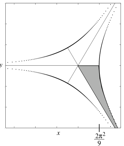
Figure 2: The geodesic submanifold $Y$.

Nakajima and Takahasi have proved that the metric on the moduli space of SU(2) monopoles and SU(n+1) monopoles broken to U(n) is equivalent to the metric on a corresponding moduli space of solutions of Nahm’s equations [18, 19]. This equivalence provides a direct method of finding metrics on monopole moduli spaces, at least for low charges where Nahm’s equations can be solved. Using the Hyperkähler quotient construction, Dancer [1], has constructed the metric on the moduli space of Nahm data corresponding to SU(3) broken to U(2) charge (2,1) monopoles denoted $M^{12}$ and by Takahasi’s proof on the equivalence of the the two metrics this gives the monopole metric. $M^{12}$ is a twelve dimensional manifold with commuting actions of Spin(3) (rotations), U(2) (unbroken gauge group), and $\hbox{\upright\hbox to0.0pt{I\hss}\kern 1.7ptR}^{3}$ (translations). Let $M^{8}$ be the quotient of $M^{12}$ by $\hbox{\upright\hbox to0.0pt{I\hss}\kern 1.7ptR}^{3}\times U(1)$ where U(1) is the center of U(2). $M^{8}$ has free commuting actions of SO(3) and SU(2)$/\hbox{\upright\hbox to0.0pt{\sans Z\hss}\kern 2.7pt{\sans Z}}_{2}$. The metric on $M^{12}$ is just the Riemannian product of the metric on $M^{8}$ with the flat metric on $\hbox{\upright\hbox to0.0pt{I\hss}\kern 1.7ptR}^{3}\times U(1)$ so the manifold $M^{8}$ describes the relative motion of the monopoles. $M^{8}$ may be quotiented by the SU(2)$/\hbox{\upright\hbox to0.0pt{\sans Z\hss}\kern 2.7pt{\sans Z}}_{2}$ action to give a manifold denoted by $N^{5}$ which has a non-free action of SO(3), corresponding to rotations. In [1], an explicit expression was given for the metric on $N^{5}$ and an implicit expression for the metric on $M^{8}$. In the Appendix the metrics on $N^{5}$ and $M^{8}$ are reexpressed in terms of coordinates $D$, $k$, on the quotient space $N^{5}/$SO(3) and left-invariant 1-forms on SO(3) corresponding to the action of SO(3) on $N^{5}$ and SO(3)$\times$SU(2)$/\hbox{\upright\hbox to0.0pt{\sans Z\hss}\kern 2.7pt{\sans Z}}_{2}$ on $M^{8}$.

Here we are interested in the interpretation of the moduli space coordinates in terms of the monopole fields. After the removal of gauge freedom, spatial translations and rotations, we are left with the two dimensional space $N^{5}/$SO(3). $N^{5}/$SO(3) may be parametrised by $D$, $k$ with $0\leq k\leq 1$ and $0\leq D<\frac{2}{3}K(k)$, where $K(k)$ denotes the first complete elliptic integral $K(k)=\int^{\frac{\pi}{2}}_{0}(1-k^{2}\sin^{2}\theta\,)^{-1/2}d\,\theta$ [1].

Figure 2 depicts a totally geodesic submanifold of $M^{8}$, $\,Y$, corresponding to monopoles which are reflection symmetric (up to a gauge transform) in each of the three Cartesian axes. $Y$ is composed of six regions each isomorphic to $N^{5}/$SO(3). The metric and geodesic flow on $Y$ was studied in [3]. In the shaded region $x,\,y$ are given in terms of $D,\,k$ by

$$x=(2-k^{2})D^{2}\,,\qquad y=-\sqrt{3}k^{2}D^{2}\;.$$ (3.1)

Similar formulae for $x,\,y$ in terms of $D,\,k$ exist in the other regions of $Y$. The origin, $x=y=0$ corresponds to the spherically symmetric monopole for which the fields are known, [2, 24]. The line segments $-\infty<x\leq 0$,$\,\,y=0$ and $0\leq x<\frac{2}{9}\pi^{2}$,$\,\,y=0$ correspond to axially symmetric monopoles, denoted in [2] as hyperbolic and trigonometric monopoles respectively, because the Nahm data involves hyperbolic and trigonometric functions. In terms of $D$ and $k$ these are lines $k=1$ and $k=0$. These line segments together correspond to a geodesic on $Y$. As $x$ varies from $-\infty$ to $\frac{2}{9}\pi^{2}$, two infinitely separated hyperbolic monopoles approach each other, collide to form the spherically symmetric monopole, which then deforms to trigonometric monopoles and approaches the axially symmetric embedded SU(2) monopole. In [2], for these cases, the Higgs field was determined along the axis of axial symmetry. The dotted boundaries of $Y$ [which is $D=\frac{2}{3}K(k)$ in $N^{5}/$SO(3)] corresponds to embedded SU(2) monopoles. $Y$ is geodesically complete and the boundary is infinitely far away in metric distance.

We want to understand the nature of the metric and the fields in different regions of $Y$. From numerical evidence in [2, 3], for large $D$, $D$ represents the separation of the monopoles. The asymptotic regions of Figure 2 (the legs of $Y$) correspond to well separated monopoles along each of the three axes. The central region corresponds to configurations of coincident or closely separated monopoles. It is interesting to try to understand the effect on the fields as one moves towards the boundary of $Y$. The coefficient of $1/r$, $(r=|{\bf x}|),$ in the asymptotic expansion of the Higgs field, $\Phi({\bf x})$, of an SU(3) monopole is $-\frac{i}{2}\mbox{diag}(-1,-1,2)$ whereas the $1/r$ coefficient of an embedded SU(2) monopole is $-\frac{i}{2}\mbox{diag}(-2,0,2)$. If one is close to the boundary of $Y$ then the fields should look like embedded SU(2) fields (since the boundary corresponds to embedded SU(2) monopoles), but with a cloud where the $1/r$ coefficient of the Higgs field changes from -$\frac{i}{2}\mbox{diag}(-2,0,2)$ to $-\frac{i}{2}\mbox{diag}(-1,-1,2)$ [2]. A useful parametrization near the boundary of $Y$ which measures approximately the radius of the cloud is given by $z=2\sqrt{\frac{D}{\rho}}$ with $\rho=2K(k)-3D$: $z$ is related to the inverse of the coordinate distance (not metric) from the boundary of $Y$. Near the boundary the expressions for the metric (A.14) may be simplified to

$$ds^{2}=dz^{2}+\frac{z^{2}}{4}(\hat{\sigma}_{1}^{2}+\hat{\sigma}_{2}^{2}+\hat{\sigma}_{3}^{2})+\frac{b^{2}}{D^{2}}dD^{2}+a^{2}\sigma_{1}^{2}+b^{2}\sigma_{2}^{2}+c^{2}\sigma_{3}^{2}\;\;+\;\;O(z^{-4})\;\;\;.$$ (3.2)

$\sigma_{i},\,\hat{\sigma}_{i}$ are left-invariant 1-forms (defined in the appendix (A.11)), corresponding to rotational and SU(2) degrees of freedom; $a^{2},\,b^{2},\,c^{2}$ are evaluated at the boundary ,$\;D=\frac{2}{3}K(k)$, giving

$$a^{2}=\frac{2K(K-E)(E-k^{\prime 2}K)}{3E}\,,\qquad b^{2}=\frac{2EK(K-E)}{3(E-k^{\prime 2}K)}\,,\qquad c^{2}=\frac{2EK(E-k^{\prime 2}K)}{3(K-E)}\,.$$ (3.3)

Here $k^{\prime 2}=1-k^{2}$ and $E(k)=\int_{0}^{\frac{\pi}{2}}(1-k^{2}\sin^{2}\theta)^{1/2}\,d\theta$.

Now, noting that (3.2) describes the flat space metric for $\hbox{\upright\hbox to0.0pt{I\hss}\kern 1.7ptR}^{4}$ and the Atiyah-Hitchin (${\cal AH}$) metric for SU(2) monopoles (with a scale factor of $1/3$) [25], we see that in the limit the metric decouples into the direct product $\hbox{\upright\hbox to0.0pt{I\hss}\kern 1.7ptR}^{4}\times{\cal AH}$. We can interpret this by saying the monopole configuration looks like an embedded charge two SU(2) monopole surrounded by a cloud, parametrized by $\hbox{\upright\hbox to0.0pt{I\hss}\kern 1.7ptR}^{4}$. In this limit the geodesics on $M^{8}$ are easy to analyse. They are given by a straight line in the $\hbox{\upright\hbox to0.0pt{I\hss}\kern 1.7ptR}^{4}$ factor and the usual geodesics on the Atiyah-Hitchin manifold. From numerical evidence in [3], it was shown that all geodesics (except for the axially symmetric monopole collision) approach the asymptotic regions of $Y$. In fact, we were able to check (using MATLAB) that generic geodesics approach the boundary of the asymptotic region, i.e. $D\rightarrow\infty$ and $D\rightarrow\frac{2}{3}K(k)$. It is interesting to ask whether similar behaviour occurs for generic geodesics on $M^{8}$ not restricted to the submanifold $Y$. From (3.2) it can be seen that if a configuration is close to the boundary and heading towards the boundary ($\dot{z}>0$) then the monopoles will continue to approach $z=\infty$. Also (3.2) suggests that the cloud will be spherically symmetric in the limit $z\rightarrow\infty$ because the coefficients of $\hat{\sigma}_{i}^{2}$ are all equal.

With the assumption that near the boundary the long-range fields are spherically symmetric we may now solve for these fields and independently verify that the $\hbox{\upright\hbox to0.0pt{I\hss}\kern 1.7ptR}^{4}$ part of the metric in (3.2) is correct. This is simplest for the axially symmetric trigonometric monopoles, ($k=0$). For such monopoles in [2], the Higgs field was given along the axis of axial symmetry. The long-range part of the Higgs field on the axis of symmetry may be found by dropping all terms exponentially small in $r$. Spherical symmetry determines the long-range Higgs field in all directions. On the axis of symmetry,

$\Phi=i$diag$(\Phi_{11},\,-\Phi_{11}-\Phi_{33},\,\Phi_{33})\,+O(e^{-6r})$ with

$$\Phi_{11}=-1+\frac{1}{D^{2}+4r^{2}}\left\{\frac{(4r^{2}-D^{2})\sin 3D-4Dr\cos 3D}{2r\sin 3D-D\cos 3D}\right\}\,,\;\;\Phi_{33}=2-\frac{4r}{4r^{2}+D^{2}}\;.$$ (3.4)

To solve the spherically symmetric BPS equations the Higgs field needs to be further truncated to

$$\Phi_{11}=-1+\frac{1}{r}\left\{\frac{r\sin 3D-D\cos 3D}{2r\sin 3D-D\cos 3D}\right\}\;,\qquad\Phi_{33}=2-\frac{1}{r}\;.$$ (3.5)

Because $D<\pi/3$ and $r$ is large this is a valid approximation. The equations may then be solved for all values of $D$. However we are only interested in configurations near the boundary $(D\rightarrow\pi/3)$ where the $\hbox{\upright\hbox to0.0pt{I\hss}\kern 1.7ptR}^{4}$ part of the metric decouples. We expand $\sin 3D,\,\cos 3D$ to order $\rho$, (here $\rho$ is $\pi-3D$ because $k=0$) and express the fields in terms of $z=2\sqrt{\frac{D}{\rho}}$. Then using [26] the spherically symmetric BPS equations may be solved to give the long-range part of the gauge field $A_{i}^{a}$ (in a gauge with a Dirac string). The singularity at the origin is not relevant here as we are only interested in the long-range fields. We find

$$\Phi(r) = i\left(\begin{array}[]{ccc}-1&0&0\\ 0&-1&0\\ 0&0&2\end{array}\right)+\frac{i}{r}\left(\begin{array}[]{ccc}\frac{z^{2}+4r}{z^{2}+8r}&0&0\\ 0&\frac{4r}{z^{2}+8r}&0\\ 0&0&-1\end{array}\right)$$ (3.12)

$${\bf A}(r,\theta) = \frac{i}{2r}\,\frac{8r}{z^{2}+8r}\left(\begin{array}[]{ccc}0&-i&0\\ i&0&0\\ 0&0&0\end{array}\right)\hat{\theta}$$ (3.16)

$$- \left\{\frac{i}{2r}\,\frac{8r}{z^{2}+8r}\left(\begin{array}[]{ccc}0&1&0\\ 1&0&0\\ 0&0&0\end{array}\right)-i\frac{\cos\theta}{r\sin\theta}\left(\begin{array}[]{ccc}1&0&0\\ 0&0&0\\ 0&0&-1\end{array}\right)\right\}\hat{\phi}$$ (3.23)

where $r$, $\theta$, $\phi$ are spherical polar coordinates. If $z$ is large enough so that $z^{2}\gg r$ then the $1/r$ coefficient in $\Phi$ is approximately $-\frac{i}{2}\mbox{diag}(-2,0,2)$. However as $r\rightarrow\infty$ the $1/r$ coefficient in $\Phi$ is $-\frac{i}{2}\mbox{diag}(-1,-1,2)$ as required. Near the boundary of $Y$ ($z\rightarrow\infty$), the change in fall-off in the $1/r$ term is extremely slow. As $r\rightarrow\infty$ with $z^{2}\ll r,\;\Phi_{11}$ may be expanded to give

$$\Phi_{11}=-i+\frac{i}{2r}+\frac{iz^{2}}{16r^{2}}\;,$$ (3.24)

so $z$ may be seen as changing the dipole term in $\Phi$. The foregoing analysis leads us to interpret $z^{2}$ as the cloud radius.

From ${\bf A}$, the magnetic field ${\bf B}$ may be found, giving

$${\bf B} = \frac{i}{2r^{2}}\left\{\left(\begin{array}[]{ccc}-1&0&0\\ 0&-1&0\\ 0&0&2\end{array}\right)-\frac{z^{2}(z^{2}+16r)}{(z^{2}+8r)^{2}}\left(\begin{array}[]{ccc}1&0&0\\ 0&-1&0\\ 0&0&0\end{array}\right)\right\}\hat{r}$$ (3.31)

$$+ \frac{4iz^{2}}{r(z^{2}+8r)^{2}}\left\{\left(\begin{array}[]{ccc}0&1&0\\ 1&0&0\\ 0&0&0\end{array}\right)\hat{\theta}+\left(\begin{array}[]{ccc}0&-i&0\\ i&0&0\\ 0&0&0\end{array}\right)\hat{\phi}\right\}\;\;.$$ (3.38)

The magnetic field is seen to be non-Abelian in the cloud region $r\approx z^{2}$. As $r\rightarrow\infty$ the non-Abelian components decay like $1/r^{3}$ leaving an Abelian magnetic field at infinity,

$${\bf B}=\frac{i}{2}\left(\begin{array}[]{ccc}-1&0&0\\ 0&-1&0\\ 0&0&2\end{array}\right)\,\frac{\hat{r}}{r^{2}}\;.$$ (3.39)

The cloud may be viewed as some form of shield for the non-Abelian magnetic field. The fields described here exhibit very similar behaviour to the fields given in [6] for the SO(5) monopole where again there is a cloud parameter describing the extent to which the long-range non-Abelian fields penetrate beyond the monopoles’ core.

Now $0\leq z<\infty$ and $k=0$ is part of a geodesic on $Y$ [1]. The kinetic energy, $T$, from the asymptotic fields obtained by varying $z$ may be calculated and compared to that from the metric (the constant of proportionality between the metric and the Lagrangian for the two monopole system is one sixth the reduced mass of a pair of monopoles, which is $\pi$). Normally one needs to add a little gauge transform to ensure that the variation of the fields is orthogonal to gauge orbits, but in this case, $D_{i}\delta A_{i}+[\Phi,\delta\Phi]=0$ is satisfied anyway with $\delta A_{i}=\dot{z}\,\partial A_{i}/\partial z\,\,$, $\delta\Phi=\dot{z}\,\partial\Phi/\partial z\;$. Thus, the kinetic energy $T$ is given by

$$T=\frac{1}{2}\int d^{3}x\left\{<\frac{\partial\Phi}{\partial z},\frac{\partial\Phi}{\partial z}>+<\frac{\partial A_{i}}{\partial z},\frac{\partial A_{i}}{\partial z}>\right\}\;\dot{z}^{2}\;,$$ (3.40)

where $<X,Y>=-2\mbox{Tr}XY\;$. One finds

$$T=\pi\dot{z}^{2}\;+\;O(z^{-4})\,\dot{z}^{2}\;.$$ (3.41)

In the limit $z\rightarrow\infty$, this formula agrees with that found from the metric (3.2), however not to $O(z^{-4})$. This means that as $z\rightarrow\infty$ all the kinetic energy is outside the core (and indirectly verifies the assumption of asymptotic spherical symmetry). The geodesic equation may be solved near the boundary to give

$$z(t)=\beta t\;,$$ (3.42)

with $\beta$ constant and total kinetic energy, $T=\pi\beta^{2}$.

For the line of hyperbolic monopoles $(k=1)$, the Higgs field was given on the axis of axial symmetry in [2]. It was seen that there is no cloud in this case. The line $k=1$ (or $z=0$) is infinitely far from the boundary and the cloud should not be expected to exist here.

The long-range fields for the 1-parameter family of trigonometric monopoles is given in (3.6), (3.7). For all points in $Y$ near the boundary the long-range fields must behave in a similar fashion, with a cloud where the $1/r$ part of the Higgs field changes from $-\frac{i}{2}$diag$(-2,0,2)$ to $-\frac{i}{2}$diag$(-1,-1,2)$. This cloud will necessarily be larger than the monopoles’ separation which is $D$. We may view the long-range fields as functions of $D$, $z$. In analogy with the trigonometric case we expect that as $z\rightarrow\infty$ the kinetic energy of the long-range fields obtained by varying the cloud parameter $z$ should equal the kinetic energy derived from the corresponding term in the metric, i.e. $\pi\dot{z}^{2}$. This is indeed the case if the long-range fields are gauge equivalent to (3.6), (3.7) for all $k$.

It is worth noting that this cloud cannot be interpreted as a kink, i.e. some region where the fields rapidly change their $1/r$ fall-off from $-\frac{i}{2}\mbox{diag}(-2,0,2)$ to $-\frac{i}{2}\mbox{diag}(-1,-1,2)$. As seen from (3.6) the change in $1/r$ fall-off in $\Phi$ is very slow as $z\rightarrow\infty$. Also the static energy density ${\cal{E}}$, $({\cal{E}}=<B^{i},\,B^{i}>)$, in this region may be easily found from (3.9) to be

$${\cal E}=\frac{4}{r^{4}}-\frac{z^{2}+2r}{2r(r+z^{2}/8)^{4}}$$ (3.43)

We see that for large $z$, $\cal{E}$ is of order $1/r^{4}$ varying from $4/r^{4}$ to $3/r^{4}$ as $r$ changes from $r\ll z^{2}$ to $r\gg z^{2}$. The energy density outside the monopole cores is small irrespective of $z$. For large $z$ the long-range fields and energy density change only slightly with $z$.

At an arbitrary point in $M^{8}$ represented by $(\Phi,\,{\bf A})$ a tangent vector may be written as $(\delta\Phi,\,\delta{\bf A})$ with $D_{i}\delta A_{i}+[\Phi,\delta\Phi]=0$, and $(\delta\Phi,\,\delta{\bf A})$ also satisfy the linearized Bogomol’nyi equations. From one such tangent vector other tangent vectors may be generated by

$$\delta^{\prime}\Phi = -\hat{\bf n}\cdot\delta{\bf A}$$ (3.44)

$$\delta^{\prime}{\bf A} = \hat{\bf n}\delta\Phi+\hat{\bf n}\times\delta{\bf A}$$

where $\hat{\bf n}$ is any constant unit vector. It is easy to see that these also satisfy the above conditions for a tangent vector. By choosing an orthonormal triplet $\hat{\bf n}_{1},\,\hat{\bf n}_{2},\,\hat{\bf n}_{3}$ we obtain four zero modes which are mutually orthogonal. Denoting by $J_{i}$ the action that takes $(\delta\Phi,\,\delta{\bf A})$ to $(-\hat{\bf n}_{i}\cdot\delta{\bf A},\,\hat{\bf n}_{i}\delta\Phi+\hat{\bf n}_{i}\times\delta{\bf A})$ it is obvious that $J_{i}J_{j}=-\delta_{ij}+\epsilon_{ijk}J_{k}$ thus giving a realisation of the hyperkähler structure on $M^{8}$. For large $z$,$\;M^{8}$ splits as a product of hyperkähler manifolds, $\cal{AH}$ and $\hbox{\upright\hbox to0.0pt{I\hss}\kern 1.7ptR}^{4}$. Thus one would expect that from the zero mode $\delta A_{i}=\delta z\,\partial A_{i}/\partial z$, $\,\delta\Phi=\delta z\,\partial\Phi/\partial z$ one may generate three other zero modes which correspond to the unbroken SU(2) action. In fact, it is not difficult to check that these zero modes may be written as

$$\delta^{\prime}A_{i} = D_{i}\,\Delta({\bf r})$$ (3.45)

$$\delta^{\prime}\Phi = [\Delta({\bf r}),\,\Phi]$$

with $\Delta({\bf r})$ in the unbroken SU(2) whose explicit form is

$$\Delta({\bf r})=\frac{8ir\delta z}{z(z^{2}+8r)}\left\{\hat{{\bf n}}\cdot\hat{\theta}\left(\begin{array}[]{ccc}0&1&0\\ 1&0&0\\ 0&0&0\end{array}\right)+\hat{{\bf n}}\cdot\hat{\phi}\left(\begin{array}[]{ccc}0&-i&0\\ i&0&0\\ 0&0&0\end{array}\right)+\hat{{\bf n}}\cdot\hat{r}\left(\begin{array}[]{ccc}1&0&0\\ 0&-1&0\\ 0&0&0\end{array}\right)\right\}\,.$$ (3.55)

The gauge rotation angle is given by $\lim_{r\rightarrow\infty}\,\parallel\Delta({\bf r})\parallel$ which is $2\delta z/z$, independent of $\hat{{\bf n}}$, where $\parallel X\parallel=\sqrt{<X,X>}\;$. This implies that the metric coefficients for the SU(2) action are isotropic for large $z$ and their norm is $z^{2}/4$ times that of the $dz^{2}$ coefficient, in agreement with (3.2).
Acknowledgments  Thanks to Conor Houghton, Bernd Schroers and especially Nick Manton for many helpful discussions. I also acknowledge the financial support of the PPARC.

Appendix A Appendix : The metric

The natural metric on the moduli space is defined by computing the $L^{2}$ norms of the zero-modes (solutions of the linearized Bogomol’nyi equations). The zero-modes must be orthogonal to little gauge transforms, which means the zero-modes $\delta\Phi$, $\delta{\bf A}_{i}$ must satisfy

$$D_{i}\delta{\bf A}_{i}+[\Phi,\delta\Phi]=0$$ (A.1)

However in most cases it is extremely difficult to compute the metric in this fashion and other techniques must be used [25, 17]. Nahm’s equations are the following system of nonlinear ordinary differential equations

$$\dot{T}_{1}+[T_{0},\,T_{1}]=[T_{2},\,T_{3}]$$ (A.2)

$$\dot{T}_{2}+[T_{0},\,T_{2}]=[T_{3},\,T_{1}]$$

$$\dot{T}_{3}+[T_{0},\,T_{3}]=[T_{1},\,T_{2}]$$

where the $T_{i}$ are matrix-valued functions on an interval of the real line parametrized by $s$. They are obtained from the self-dual Yang-Mills equations in four dimensions by imposing translational invariance in three dimensions just as the Bogomol’nyi equations are obtained by imposing translational invariance in one dimension. It is known that solutions to Nahm’s equations with certain boundary conditions are in 1-1 correspondence with monopoles via the Atiyah-Drinfeld-Hitchin-Manin- (ADHM) Nahm transform. The boundary conditions of Nahm’s equations determine what gauge group the monopole is in. This transform is known to be an isometry for SU(n+1) broken to U(n) [18, 19] (this includes SU(2) monopoles) and is believed to be true generally.

Nahm data corresponding to Dancer monopoles are given by the space ${\cal C}$ of quadruples ($T_{0}\,,T_{1}\,,T_{2}\,,T_{3}$) where

(i) $T_{u}$ ($u=0,\,1,\,2,\,3)$ are functions defined on the interval $[0,\,3]$ taking values in the Lie algebra of U(2).

(ii) $T_{0}$ is analytic on $[0,\,3]$. $T_{1}$, $T_{2}$, $T_{3}$ are analytic on $(0,\,3]$ with simple poles at $s=0$ of residue $\frac{i}{2}\tau_{1}$, $\frac{i}{2}\tau_{2}$, $\frac{i}{2}\tau_{3}$, where $\tau_{i}$ are the Pauli matrices.

(iii) The $T_{i}$ satisfy Nahm’s equations.

Nahm data for embedded SU(2) monopoles are as above except now the $T_{i}$ also have poles at $s=3$. Let $G^{0}_{0}$ be the group of analytic U(2)-valued functions on $[0,3]$ which are the identity at $s=0,\,3$. This group acts on ${\cal C}$ in the following manner

$$T_{0} \rightarrow gT_{0}g^{-1}-\frac{dg}{ds}g^{-1}$$ (A.3)

$$T_{i} \rightarrow gT_{i}g^{-1}\;,\;\;\;\;\;\;\;\;\;(i=1,\,2,\,3)\;.$$

The moduli space of Nahm data, denoted $M^{12}$, is the quotient of ${\cal C}$ by $G^{0}_{0}$. $M^{12}$ has the following isometric group actions.

(a) There is an action of $\hbox{\upright\hbox to0.0pt{I\hss}\kern 1.7ptR}^{3}$ on $M^{12}$, given by

$$T_{i}\rightarrow T_{i}-i\lambda_{i}\mbox{Id}\qquad(i=1,2,3)\,,$$ (A.4)

where $(\lambda_{1},\lambda_{2},\lambda_{3})\in\hbox{\upright\hbox to0.0pt{I\hss}\kern 1.7ptR}^{3}\,.$

(b) Let $G_{0}$ be the group of analytic U(2)-valued functions on $[0,3]$ which are the identity at $s=0$. This acts on ${\cal C}$ as in (A.3) with $g(3)=P$ say. This action descends to an action of $G_{0}/G_{0}^{0}\cong$U(2) on $M^{12}.$

(c) There is a Spin(3) action on $M^{12}$ induced from the following action on ${\cal C}$. Let $R\in$ SU(2) descend to $(R_{ij})\in$ SO(3). $g$ is an analytic U(2)-valued function on $[0,3]$ which satisfies $g(0)=R,\;g(3)=\,$Id. Then the Spin(3) action is defined by

$$T_{0} \rightarrow gT_{0}g^{-1}-\frac{dg}{ds}g^{-1}$$ (A.5)

$$T_{i} \rightarrow g(\,\sum R_{ij}T_{j}\,)g^{-1}\;,\;\;\;\;\;\;\;\;\;(i=1,\,2,\,3)\,.$$

$M^{8}$ is defined as the quotient of $M^{12}$ by $\hbox{\upright\hbox to0.0pt{I\hss}\kern 1.7ptR}^{3}\times$U(1) where the U(1) is the center of U(2) and $N^{5}$ is the quotient of $M^{8}$ by the SU(2) action. Using the SU(2) action to set $T_{0}$ to zero, Nahm’s equations become $\dot{T}_{1}=[T_{2},\,T_{3}]$ + cyclic.

We may now use the Spin(3) action to set $T_{i}=-\frac{i}{2}f_{i}\tau_{i}$ (no sum on $i$) and Nahm’s equations reduce to the Euler top equations

$$\dot{f}_{1}=f_{2}f_{3}\;\;+\mbox{cyclic}$$ (A.6)

whose solution is

$$f_{1}(s)=-\frac{Dcn_{k}(Ds)}{sn_{k}(Ds)}\,,\qquad f_{2}(s)=-\frac{Ddn_{k}(Ds)}{sn_{k}(Ds)}\,,\qquad f_{3}(s)=-\frac{D}{sn_{k}(Ds)}\;.$$ (A.7)

$D$, $k$ are coordinates on the quotient space $N^{5}/$SO(3). In order to express the metric it is useful to define $X,\,g_{1},\,g_{2}$ by

$$X(k,D)=f_{1}(3)f_{2}(3)f_{3}(3)\,,\qquad g_{1}(k,D)=\int_{0}^{3}\frac{1}{f_{2}^{2}}\,ds\,,\qquad g_{2}(k,D)=\int_{0}^{3}\frac{1}{f_{3}^{2}}\,ds\;.$$ (A.8)

By the isometry proved in [19] the metric on the moduli space $M^{12}$ induced from the natural $L^{2}$ metric on ${\cal C}$ gives the metric on the moduli space of charge $(2,\,1)$ SU(3) monopoles. In [1], an explicit expression was given for the metric on $N^{5}$ and an implicit expression for the metric on $M^{8}$. Here we want an explicit expression for the metric in terms of $dD,\,dk$ and left-invariant 1-forms corresponding to the SO(3)$\times$SO(3) action. In [1] the metric on $N^{5}$ was expressed in terms of coordinates $\alpha_{i}$ which are related to the inner products of the Nahm matrices. Explicitly,

$$\alpha_{1} = <T_{1},T_{1}>-<T_{2},T_{2}>\;,$$ (A.9)

$$\alpha_{2} = <T_{1},T_{1}>-<T_{3},T_{3}>\;,$$

$$\alpha_{3} = <T_{1},T_{2}>\;,$$

$$\alpha_{4} = <T_{1},T_{3}>\;,$$

$$\alpha_{5} = <T_{2},T_{3}>\,,$$

and again $<X,Y>=-2\mbox{Tr}XY$. $\alpha_{i}$ may be expressed in terms of $D$, $k$ and an SO(3) matrix $(R_{ij})$. The SO(3) symmetry of the metric means that it may be written in the form

$$ds^{2}=A(k,D)dk^{2}+2B(k,D)dkdD+C(k,D)dD^{2}+a_{ij}(k,D)\sigma_{i}\sigma_{j}$$ (A.10)

with $\sigma_{i}$ left-invariant 1-forms on SO(3) defined by $\frac{i}{2}\tau_{i}\sigma_{i}=R^{\dagger}\,dR$ where $R\in$SU(2) descends to $(R_{ij})$. If $\theta$, $\phi$, $\psi$ are the usual Euler angles for SO(3), with $0\,\leq\,\theta\,\leq\,\pi$, $0\,\leq\,\phi\,\leq\,2\pi$, $0\,\leq\,\psi\,\leq\,2\pi$, then,

$$\sigma_{1} = -\sin\psi\,d\theta+\cos\psi\,\sin\theta\,d\phi$$ (A.11)

$$\sigma_{2} = \cos\psi\,d\theta+\sin\psi\,\sin\theta\,d\phi$$

$$\sigma_{3} = d\psi+\cos\theta\,d\phi\;.$$

The coefficients $A,B,C$ are known from [3], however it is easier to express the metric in terms of $\tilde{\alpha}_{1}=-(1-k^{2})D^{2},\;\tilde{\alpha}_{2}=-D^{2}$, which are $\alpha_{1},\,\alpha_{2}$ restricted to $N^{5}/$SO(3). $a_{ij}$ can be found by letting $R=1+\delta$ with all entries in $\delta$ close to zero and expressing the metric in terms of the invariant 1-forms at this point. Hence (A.10) may be written as

$$ds^{2}=\frac{1}{4}\left\{X(g_{1}d\tilde{\alpha}_{1}+g_{2}d\tilde{\alpha}_{2})^{2}+g_{1}d\tilde{\alpha}_{1}^{2}+g_{2}d\tilde{\alpha}_{2}^{2}\right\}+a_{1}\sigma_{1}^{2}+a_{2}\sigma_{2}^{2}+a_{3}\sigma_{3}^{2}$$ (A.12)

with

$$a_{1} = k^{4}D^{4}\frac{g_{1}g_{2}}{g_{1}+g_{2}}$$ (A.13)

$$a_{2} = D^{4}\left\{g_{2}+\frac{Xg_{2}^{2}}{Xg_{1}+1}\right\}$$

$$a_{3} = D^{4}(1-k^{2})^{2}\left\{g_{1}+\frac{Xg_{1}^{2}}{Xg_{2}+1}\right\}\;.$$

$a_{ij}$ is diagonal due to a $\hbox{\upright\hbox to0.0pt{\sans Z\hss}\kern 2.7pt{\sans Z}}_{2}\times\hbox{\upright\hbox to0.0pt{\sans Z\hss}\kern 2.7pt{\sans Z}}_{2}$ symmetry on $N^{5}$. The coefficients of the metric depend only on $D$, $k$. The metric on $M^{8}$ will contain the left-invariant 1-forms $\sigma_{i},\check{\sigma}_{i}$, corresponding to the SO(3)$\times$SO(3) action where $\check{\sigma}_{i}$ is defined by $\frac{i}{2}\tau_{i}\check{\sigma}_{i}=P^{\dagger}\,dP$ and again $P\in$ SU(2) descends to $(P_{ij})\in$ SO(3). $\hat{\sigma}_{i}$ which appeared in Section $3$ will be defined below in terms left $and$ right-invariant 1-forms corresponding to $P,\,R$. The metric coefficients on $M^{8}$ in [1] are determined by orthogonality conditions depending on $D$, $k$ and $(R_{ij})$, $(P_{ij})$ in SO(3). These may be solved for $(R_{ij})$, $(P_{ij})$ in the neighbourhood of the identity to get the metric in this region in terms of $d\tilde{\alpha}_{1}$, $d\tilde{\alpha}_{2}$, $\sigma_{i},\check{\sigma}_{i}$ and again this holds everywhere in $M^{8}$ due to the SO(3)$\times$SO(3) symmetry of the metric. We have

$$ds^{2} = \frac{1}{4}\left\{X(g_{1}d\tilde{\alpha}_{1}+g_{2}d\tilde{\alpha}_{2})^{2}+g_{1}d\tilde{\alpha}_{1}^{2}+g_{2}d\tilde{\alpha}_{2}^{2}\right\}+a_{1}\sigma_{1}^{2}+a_{2}\sigma_{2}^{2}+a_{3}\sigma_{3}^{2}$$

$$+ \left\{b_{1}\sigma_{1}-c_{1}(\frac{f_{3}(3)}{f_{2}(3)}\sigma_{1}-\check{\sigma}_{1})\right\}^{2}+\left\{b_{2}\sigma_{2}-c_{2}(\frac{f_{1}(3)}{f_{3}(3)}\sigma_{2}-\check{\sigma}_{2})\right\}^{2}$$

$$+ \left\{b_{3}\sigma_{3}-c_{3}(\frac{f_{1}(3)}{f_{2}(3)}\sigma_{3}-\check{\sigma}_{3})\right\}^{2}$$

$a_{i}$ are as before, and

$$b_{1} = k^{2}D^{2}\sqrt{\frac{g_{1}^{2}}{(g_{1}+g_{2})(Xg_{1}+Xg_{2}+1)}}\;,\quad c_{1}=f_{2}(3)f_{3}(3)\sqrt{\frac{g_{1}+g_{2}}{Xg_{1}+Xg_{2}+1}},$$ (A.15)

$$b_{2} = \frac{g_{2}D^{2}}{\sqrt{Xg_{1}^{2}+g_{1}}}\;,\quad\qquad\qquad\qquad\qquad\quad\;\,c_{2}=\frac{\sqrt{Xg_{1}^{2}+g_{1}}}{f_{2}(3)g_{1}}\;,$$

$$b_{3} = \frac{g_{1}D^{2}k^{\prime 2}}{\sqrt{Xg_{2}^{2}+g_{2}}}\;,\quad\qquad\qquad\qquad\qquad\quad\;\,c_{3}=\frac{\sqrt{Xg_{2}^{2}+g_{2}}}{f_{3}(3)g_{2}}\;.$$

Again $b_{i}$, $c_{i}$ depend only on $D$, $k$. $D$ satisfies $0\leq D<\frac{2}{3}K(k)$ . The manifold thus has a boundary $D=\frac{2}{3}K(k)$ corresponding to Nahm data which are singular at $s=0$ and $s=3$. As one approaches the boundary on $M^{8}$ the metric (A.14) becomes

$$ds^{2} = dz^{2}+\frac{z^{2}}{4}\left\{(\sigma_{1}-\check{\sigma}_{1})^{2}+(\sigma_{2}+\check{\sigma}_{2})^{2}+(\sigma_{3}+\check{\sigma}_{3})^{2}\right\}$$

$$+ \frac{b^{2}}{D^{2}}dD^{2}+a^{2}\sigma_{1}^{2}+b^{2}\sigma_{2}^{2}+c^{2}\sigma_{3}^{2}\;+\;O(z^{-4})\;,$$

with $a^{2},\,b^{2},\,c^{2}$ defined in (3.3). As stated previously the second line in (A.16) is the Atiyah-Hitchin metric. We now do a coordinate transform so that the first line in (A.16) is explicitly seen to be the flat metric on $\hbox{\upright\hbox to0.0pt{I\hss}\kern 1.7ptR}^{4}$. We redefine the Spin(3) action, (A.5), so that $g(3)=e^{\frac{i\pi}{2}\sigma_{1}}R^{\dagger}e^{\frac{i\pi}{2}\sigma_{1}}$ (the purpose of the $e^{\frac{i\pi}{2}\sigma_{1}}$ terms is to change the signs of $\check{\sigma}_{2},\,\check{\sigma}_{3})$. $\hat{\sigma}_{i}$ which appears in (3.2) is defined by $\frac{i}{2}\tau_{i}\hat{\sigma}_{i}=X^{\dagger}dX$ where $X=Pe^{\frac{i\pi}{2}\sigma_{1}}R^{\dagger}e^{\frac{i\pi}{2}\sigma_{1}}$. Expressed in terms of 1-forms corresponding to the matrices $R,\,P$ the metric will now contain both left and right-invariant 1-forms but for large cloud parameter (A.16) now takes the simple form given in (3.2), essentially because $\sigma_{1}^{2}+\sigma_{2}^{2}+\sigma_{3}^{2}$ is independent of whether $\sigma_{i}$ is a left or right-invariant 1-form. The point is that $g(3)$ can be chosen arbitrarily and we choose it as above so that the form of the metric near the boundary, (A.16), takes an especially simple form.

References

- [1] A.S. Dancer, Commun. Math. Phys. 158 (1993) 545.
- [2] A.S. Dancer, Nonlinearity 5 (1992) 1355.
- [3] A.S. Dancer and R.A. Leese, Proc. R. Soc. 440 (1993) 421.
- [4] A.S. Dancer and R.A. Leese, Phys. Lett. B390 (1997) 252.
- [5] J. Gauntlett and D. Lowe, Nucl. Phys. B472 (1996) 194. K. Lee, E. J. Weinberg, P. Yi, Phys. Lett. B376 (1996) 97.
- [6] K. Lee, E. J. Weinberg, P. Yi, Phys. Rev. D54 (1996) 6351.
- [7] S.A. Connell, The dynamics of the SU(3) charge (1,1) magnetic monopole, University of South Australia preprint.
- [8] K. Lee, E. J. Weinberg, P. Yi, Phys. Rev. D54 (1996) 1633.
- [9] G.W. Gibbons and P. Rychenkova, hep-th/9608085, to appear in Commun. Math. Phys.
- [10] P. Goddard, J. Nuyts and D. Olive, Nucl. Phys. B125 (1977) 1.
- [11] A. Abouelsaood, Phys. Lett. 125B (1983) 467.
- [12] A. Abouelsaood, Nucl. Phys. B226 (1983) 309.
- [13] P. Nelson and A. Manohar, Phys. Rev. Lett. 50 (1983) 943. A. Balachandran, G. Marmo, M. Mukunda, J. Nilsson, E. Sudarshan and F. Zaccaria, Phys. Rev. Lett. 50 (1983) 1553.
- [14] M.C. Bowman, Phys. Rev. D32 (1985) 1569.
- [15] M. K. Murray, Comm. Math. Phys 125 (1989) 661.
- [16] E. J. Weinberg, Nucl. Phys. B167 (1980) 500.
- [17] W. Nahm, in Monopoles in Quantum Field Theory, N. Craigie et al. (eds.) Singapore: World Scientific (1982).
- [18] H. Nakajima, in Sanda 1990, Proceeedings, Einstein metrics and Yang-Mills connections.
- [19] M. Takahasi, Phd. Thesis, University of Tokyo.
- [20] F. Englert and P. Windey, Phys. Rev. D14 (1976) 2728.
- [21] F. A. Bais, Phys. Rev. D18 (1978) 1206.
- [22] J. Hurtubise, Commum. Math. Phys 120 (1989) 613.
- [23] G. Chalmers, Multi Monopole Moduli Spaces for Gauge Group, hep-th/9605182.
- [24] F. A. Bais and D. Wilkinson, Phys. Rev. D19 (1979) 2410.
- [25] M. F. Atiyah and N. J. Hitchin, The geometry and dynamics of magnetic monopoles, Princeton University Press 1988.
- [26] N.S. Manton, Ann. Phys. 132 (1981) 108.