A doubled discretisation of abelian Chern–Simons theory

Abstract

A new discretisation of a doubled, i.e. BF, version of the pure abelian Chern–Simons theory is presented. It reproduces the continuum expressions for the topological quantities of interest in the theory, namely the partition function and correlation function of Wilson loops. Similarities with free spinor field theory are discussed which are of interest in connection with lattice fermion doubling.

The abelian Chern–Simons (CS) theory [1, 2, 3] is an important topological field theory in three dimensions. It provides the topological structure of topologically massive (abelian) gauge theory [2] and, in the euclidean metrics, provides a useful theoretical framework for the description of interesting phenomena in planar condensed matter physics as, for example, fractional statistics particles [5], the quantum Hall effect, and high $T_{c}$ superconductivity [6]. It is also essentially the same as the weak coupling (large $k$) limit of the non-abelian CS gauge theory, a solvable yet highly non-trivial topological quantum field theory [3]. In this paper we describe a discretisation of the abelian CS theory which reproduces the topological quantities of interest after introducing a field doubling in the theory. This doubling leads to the abelian Chern–Simons action being replaced by the action for the so-called abelian BF gauge theory ((2) below), in which the correlation function of Wilson loops and partition function become the square and norm-square respectively of what they originally were. Note that discretising the theory is not the same as putting it on a lattice in the usual way. Instead, it involves using a lattice to construct a discrete analogue of the theory which reproduces the key topological quantities and/or features, without having to take a continuum limit. A detailed version of this work [7] will be published elsewhere.

We take the spacetime to be euclidean ${\bf R}^{3}$ (the case of general 3-manifolds is dealt with in [7]). The abelian CS action for gauge field $A\!=\!A_{\mu}dx^{\mu}$ can be written as

$$S(A)=\lambda\int_{\bf R^{3}}dx\,\epsilon_{\mu\nu\rho}A_{\mu}\partial_{\nu}A_{\rho}=\lambda\int_{\bf R^{3}}A\wedge{}dA=\lambda\langle{}A\,,(\ast{}d)A\rangle$$ (1)

where $\lambda$ is the coupling parameter, $d$ is the exterior derivative, $\ast$ is the Hodge star operator, and $\langle\cdot\,,\cdot\rangle$ is the inner product in the space of 1-forms determined by euclidean metric in ${\bf R}^{3}$. All the ingredients the last expression in (1) have natural lattice analogues (as we will see explicitly below); however the lattice analogue of the operator $\ast$ is the duality operator, which maps between cells of the lattice $K$ and cells of the dual lattice $\widehat{K}$. To accommodate this feature we introduce a new gauge field $A^{\prime}$ and consider a doubled version of the action (1):

$$\widetilde{S}(A,A^{\prime})\,\equiv\,\lambda\langle\left({A\atop A^{\prime}}\right)\,,\,\left({0\atop\ast{}d}\;{\ast{}d\atop 0}\right)\left({A\atop A^{\prime}}\right)\rangle=2\lambda\int_{\bf R^{3}}A^{\prime}\wedge{}dA$$ (2)

This is the action of the so-called abelian BF gauge theory [4]. In this theory the correlation function of framed Wilson loops can be considered: A framed loop is a closed ribbon which we denote by $(\gamma,\gamma^{\prime})$ where $\gamma$ and $\gamma^{\prime}$ are the two boundary loops of the ribbon. The Wilson correlation function of oriented framed loops $(\gamma^{(1)},\gamma^{(1)}{}^{\prime}),\dots,(\gamma^{(r)},\gamma^{(r)}{}^{\prime})$ is

$$\langle(\gamma^{(1)},\gamma^{(1)}{}^{\prime}),\dots,(\gamma^{(r)},\gamma^{(r)}{}^{\prime})\rangle\equiv\widetilde{Z}(\lambda)^{-1}\int_{{\cal A}\times{\cal A}}{\cal D\/}A{\cal D\/}A^{\prime}\,[\prod_{l=1}^{r}\Bigl{(}\,e^{i\oint_{\gamma^{(l)}}A}\Bigr{)}\Bigl{(}\,e^{i\oint_{\gamma^{(l)}{}^{\prime}}A^{\prime}}\Bigr{)}]\,e^{i\widetilde{S}(A,A^{\prime})}$$ (3)

This can be formally evaluated using standard techniques [4] to obtain

$$\langle(\gamma^{(1)},\gamma^{(1)}{}^{\prime}),\dots,(\gamma^{(r)},\gamma^{(r)}{}^{\prime})\rangle=\exp\Bigl{(}{\textstyle\frac{-i}{2\lambda}}\Bigl{(}\,\sum_{l\neq{}m}L(\gamma^{(l)},\gamma^{(m)})+\sum_{l=1}^{r}L(\gamma^{(l)},\gamma^{(l)}{}^{\prime})\Bigr{)}\Bigr{)}$$ (4)

where $L(\gamma,\gamma^{\prime})$ denotes the Gauss linking number of $\gamma$ and $\gamma^{\prime}$. The partition function of this theory,

$$\widetilde{Z}(\lambda)\equiv\int_{{\cal A}\times{\cal A}}{\cal D\/}A{\cal D\/}A^{\prime}\,e^{i\widetilde{S}(A,A^{\prime})}\,,$$ (5)

is also a quantity of topological interest. After compactifying the spacetime to $S^{3}$ and imposing the the covariant gauge-fixing condition

$$d^{\dagger}A=0\qquad,\qquad{}d^{\dagger}A^{\prime}=0\ ,$$ (6)

(where $d^{\dagger}$ is the adjoint of $d$) the partition function can be formally evaluated as in [1] (see also [8]) to obtain

$$\widetilde{Z}(\lambda)=\det(\phi_{0}^{\dagger}\phi_{0})^{-1}\det{}^{\prime}(d_{0}^{\dagger}d_{0})\det{}^{\prime}\Bigl{(}{\textstyle\frac{-i\lambda}{\pi}\left({0\atop\ast{}d}\;{\ast{}d\atop 0}\right)}\Bigr{)}^{-1/2}$$ (7)

where we denote by $d_{q}$ the restriction of $d$ to the space $\Omega^{q}(S^{3})$ of $q$-forms, and $\phi_{0}:{\bf R}\to\Omega^{0}(S^{3})$ maps $r\!\in\!{\bf R}$ to the constant function equal to $r$. In this expression $\det{}^{\prime}(d_{0}^{\dagger}d_{0})$ is the Faddeev–Popov determinant corresponding to (6) and $\det(\phi_{0}^{\dagger}\phi_{0})^{-1}$ ($=V(S^{3})^{-1}$) is a “ghosts for ghosts” determinant which arises because constant gauge transformations act trivially on the gauge fields. The determinants in (7) are regularised via zeta-regularisation as in [1, 8]. Using Hodge duality and the techniques of [1, 8] we can rewrite (7) as

$$\widetilde{Z}(\lambda)=\Bigl{(}{\textstyle\frac{\lambda}{\pi}}\Bigr{)}^{-1}\tau_{RS}(S^{3};d)$$ (8)

(the general phase factor of [8, eq.(6)] is trivial here since the operator in (2) has symmetric spectrum) where

$$\tau_{RS}(S^{3};d)=\det(\phi_{0}^{\dagger}\phi_{0})^{-1/2}\det(\phi_{3}^{\dagger}\phi_{3})^{1/2}\prod_{q=0}^{2}\det{}^{\prime}(d_{q}^{\dagger}d_{q})^{\frac{1}{2}(-1)^{q}}$$ (9)

is the Ray–Singer torsion of $d$ [9] (see in particular §3 of the second paper in [9]). (In (9) $\phi_{3}:{\bf R}\to\Omega^{3}(S^{3})$ maps $r\!\in\!{\bf R}$ to the harmonic 3-form $\omega$ with $\int_{S^{3}}\omega\!=\!r$ and we have used $\det(\phi_{3}^{\dagger}\phi_{3})\!=\!V(S^{3})^{-1}\!=\!\det(\phi_{0}^{\dagger}\phi_{0})^{-1}$ [7].) The Ray–Singer torsion is a topological invariant of $S^{3}\,$, i.e. it is independent of the metric on $S^{3}$ used to construct $\ast$ and $\langle\cdot\,,\cdot\rangle$ in (2), $d^{\dagger}$ in (6), and $\phi_{0}^{\dagger}$ in (7). The physical significance of this is as follows: When compactifying ${\bf R}^{3}$ to $S^{3}\approx{\bf R}^{3}\cup\{\infty\}$ (e.g. via stereographic projection) the euclidean metric on ${\bf R}^{3}$ must be deformed towards infinity in order that it extend to a well-defined metric on $S^{3}$. The topological invariance of $\tau_{RS}(S^{3},d)$ means that the resulting partition function (8) is independent of how this deformation is carried out. In fact $\tau_{RS}(S^{3},d)\!=\!1$ (the argument for this will be given below) so $\widetilde{Z}(\lambda)\!=\!\pi/\lambda$. If ${\bf R}^{3}$ is compactified in a topologically more complicated way, leading to a general closed oriented 3-manifold $M\,$, then the preceding derivation of (8) continues to hold (with $S^{3}$ replaced by $M$) if $H^{1}(M)\!=\!0$ and can be generalised if $H^{1}(M)\neq 0$ [7]. For example, if $M$ is a lens space $L(p,q)$ then $\tau_{RS}(L(p,q),d)\!=\!1/p$ and $\widetilde{Z}(\lambda)\!=\!\pi/p\lambda$.

We will construct a discrete version of the doubled theory $\widetilde{S}(A,A^{\prime})$ which reproduces the continuum expressions (4) and (8) for the correlation function of framed Wilson loops and partition function respectively. Let $K$ be a lattice decomposition of ${\bf R}^{3}$ which, for convenience, we take to be cubic. It is well-known [10, 11] that the space $\Omega^{p}$ of antisymmetric tensor fields of degree $p$ (i.e. $p$-forms) has a discrete analogue, the space $C^{p}(K)$ of $p$-cochains (i.e. ${\bf R}$-valued functions on the $p$-cells of $K$), in particular $C^{1}(K)$ is the analogue of the space ${\cal A}\!=\!\Omega^{1}$ of gauge fields. The space $C_{p}(K)$ of $p$-chains (i.e. formal linear combinations over ${\bf R}$ of oriented $p$-cells) has a canonical inner product $\langle\cdot\,,\cdot\rangle$ defined by requiring that the $p$-cells be orthonormal; this allows to identify $C_{p}(K)$ with its dual space $C^{p}(K)$ so we will speak only of $C_{p}(K)$ in the following. The analogue of $d$ is the coboundary operator $d^{K}:C_{p}(K)\to{}C_{p+1}(K)\,$, i.e. the adjoint of the boundary operator $\partial^{K}$. The new feature of our discretisation is that we also use the (co)chain spaces $C_{q}(\widehat{K})$ associated with the dual lattice $\widehat{K}$ (i.e. the cubic lattice whose vertices are the centres of the 3-cells of $K$). The cells of $K$ and $\widehat{K}$ are related by the duality operator $\ast^{K}\,$, defined in Fig. 1. An orientation for a $p$-cell $\alpha$ determines an orientation for the dual $(3\!-\!p)$-cell $\ast^{K}\alpha$ by requiring that the product of the orientations of $\alpha$ and $\ast^{K}\alpha$ coincides with the standard orientation of ${\bf R}^{3}$. Thus the duality operator $\ast^{K}$ determines a linear map $\ast^{K}:C_{p}(K)\stackrel{{\scriptstyle\simeq}}{{\to}}C_{3-p}(\widehat{K})\,$; this is the discrete analogue of the Hodge star operator $\ast$ in (1)–(2). Set $\ast^{\widehat{K}}\equiv(\ast^{K})^{\dagger}\!=\!(\ast^{K})^{-1}$. The discrete theory is now constructed by

$$(A,A^{\prime})\in{\cal A}\times{\cal A} \longrightarrow (a,a^{\prime})\in{}C_{1}(K)\times{}C_{1}(\widehat{K})$$ (10)

$$\widetilde{S}(A,A^{\prime})\,\equiv\,\lambda\Big{\langle}\left({A\atop A^{\prime}}\right)\,,\,\left({0\atop\ast{}d}\;{\ast{}d\atop 0}\right)\left({A\atop A^{\prime}}\right)\Big{\rangle} \longrightarrow \widetilde{S}_{K}(a,a^{\prime})\,\equiv\,\lambda\Big{\langle}\left({a\atop a^{\prime}}\right)\,,\,\left({0\atop\ast^{K}d^{K}}\;{\ast^{\widehat{K}}d^{\widehat{K}}\atop 0}\right)\left({a\atop a^{\prime}}\right)\Big{\rangle}$$ (11)

The discrete action $S_{K}(a,a^{\prime})$ is invariant under $a\to{}a\!+\!d^{K}b\,$, $\;a^{\prime}\to{}a^{\prime}\!+\!d^{\widehat{K}}b^{\prime}$ for all $(b,b^{\prime})\in{}C_{0}(K)\times{}C_{0}(\widehat{K})$ since $d^{K}d^{K}\!=\!0$ and $d^{\widehat{K}}d^{\widehat{K}}\!=\!0\,$; this is the discrete analogue of the gauge invariance of the continuum theory.

Framed Wilson loops fit naturally into this discrete setup: The framed loops are taken to be ribbons $(\gamma_{K},\gamma_{\widehat{K}})$ where one boundary loop $\gamma_{K}$ is an edge loop in the lattice $K$ and the other boundary loop $\gamma_{\widehat{K}}$ is an edge loop in the dual lattice $\widehat{K}$. (It is always possible to find such a framing of an edge loop $\gamma_{K}$ [7].) There is a natural discrete version of line integrals:

$$\oint_{\gamma_{K}}A\ \longrightarrow\ \langle\underline{\gamma}_{K}\,,a\rangle\qquad,\qquad\oint_{\gamma_{\widehat{K}}}A^{\prime}\ \longrightarrow\ \langle\underline{\gamma}_{\widehat{K}}\,,a^{\prime}\rangle$$ (12)

where $\underline{\gamma}_{K}\in{}C_{1}(K)$ denotes the sum of the 1-cells in $K$ making up $\gamma_{K}\,$, and $\underline{\gamma}_{\widehat{K}}\in{}C_{1}(\widehat{K})$ denotes the sum of the 1-cells in $\widehat{K}$ making up $\gamma_{\widehat{K}}$. Then the correlation function of non-intersecting oriented framed edge loops $(\gamma_{K}^{(1)},\gamma_{\widehat{K}}^{(1)}),\dots,(\gamma_{K}^{(r)},\gamma_{\widehat{K}}^{(r)})$ in the discrete theory is

$$\langle(\gamma_{K}^{(1)},\gamma_{\widehat{K}}^{(1)}),\dots,(\gamma_{K}^{(r)},\gamma_{\widehat{K}}^{(r)})\rangle\equiv\widetilde{Z}_{K}(\lambda)^{-1}\int_{C_{1}(K)\times{}C_{1}(\widehat{K})}{\cal D\/}a{\cal D\/}a^{\prime}\,[\prod_{l=1}^{r}\Bigl{(}\,e^{i\langle\underline{\gamma}_{K}^{(l)}\,,a\rangle}\Bigr{)}\Bigl{(}\,e^{i\langle\underline{\gamma}_{\widehat{K}}^{(l)}\,,a^{\prime}\rangle}\Bigr{)}]\,e^{i\widetilde{S}_{K}(a,a^{\prime})}$$ (13)

A formal evaluation analogous to the evaluation of (3) leading to (4) gives

$$\langle(\gamma_{K}^{(1)},\gamma_{\widehat{K}}^{(1)}),\dots,(\gamma_{K}^{(r)},\gamma_{\widehat{K}}^{(r)})\rangle = \exp\Bigl{(}{\textstyle\frac{-i}{4\lambda}\Big{\langle}\biggl{(}{\underline{\gamma}_{K}^{(1)}+\dots+\underline{\gamma}_{K}^{(r)}\atop\underline{\gamma}_{\widehat{K}}^{(1)}+\dots+\underline{\gamma}_{\widehat{K}}^{(r)}}\biggr{)}\,,\,\left({0\atop\ast^{K}d^{K}}\;{\ast^{\widehat{K}}d^{\widehat{K}}\atop 0}\right)^{\!-1}\biggl{(}{\underline{\gamma}_{K}^{(1)}+\dots+\underline{\gamma}_{K}^{(r)}\atop\underline{\gamma}_{\widehat{K}}^{(1)}+\dots+\underline{\gamma}_{\widehat{K}}^{(r)}}\biggr{)}\Big{\rangle}}\Bigr{)}$$ (14)

$$= \exp\Bigl{(}{\textstyle\frac{-i}{2\lambda}}\sum_{l,m=1}^{r}\langle\underline{\gamma}_{K}^{(l)}\,,(\ast^{K}d^{K})^{-1}\underline{\gamma}_{\widehat{K}}^{(m)}\rangle\Bigr{)}$$ (15)

where we have used $(\ast^{K}d^{K})^{\dagger}\!=\!\ast^{\widehat{K}}d^{\widehat{K}}$. To show that this coincides with the continuum expression (4) we must show that for any oriented edge loop $\gamma_{K}$ in $K$ and oriented edge loop $\gamma_{\widehat{K}}$ in $\widehat{K}\,$,

$$\langle\underline{\gamma}_{K}\,,(\ast^{K}d^{K})^{-1}\underline{\gamma}_{\widehat{K}}\rangle\;=\,L(\gamma_{K},\gamma_{\widehat{K}})\,.$$ (16)

Then taking $\gamma_{K}\!=\!\gamma_{K}^{(l)}$ and $\gamma_{\widehat{K}}\!=\!\gamma_{\widehat{K}}^{(m)}$ in (16) and substituting in (15) reproduces the continuum expression (4). To derive (16) we recall that the linking number of $\gamma_{K}$ and $\gamma_{\widehat{K}}$ can be characterised as follows. Let $D$ be a surface in ${\bf R}^{3}$ with $\gamma_{K}$ as its boundary, and such that all intersections of $D$ with $\gamma_{\widehat{K}}$ are transverse, then

$$L(\gamma_{K},\gamma_{\widehat{K}})=\sum_{D\,\cap\,\gamma_{\widehat{K}}}\pm 1$$ (17)

where the sign of $\pm 1$ for a given intersection of $D$ and $\gamma_{\widehat{K}}$ is $+$ if the product of the orientations of $D$ (induced by the orientation of $\gamma_{K}$) and $\gamma_{\widehat{K}}$ at the intersection coincides with the standard orientation of ${\bf R}^{3}\,$, and $-$ otherwise. We now show that the l.h.s. of (16) coincides with (17). First note that

$$\langle\underline{\gamma}_{K}\,,(\ast^{K}d^{K})^{-1}\underline{\gamma}_{\widehat{K}}\rangle\;=\;\langle((\ast^{K}d^{K})^{-1})^{\dagger}\underline{\gamma}_{K}\,,\underline{\gamma}_{\widehat{K}}\rangle\;=\;\langle\ast^{K}(\partial^{K})^{-1}\underline{\gamma}_{K}\,,\underline{\gamma}_{\widehat{K}}\rangle\,.$$ (18)

Choose a surface $D_{K}$ in ${\bf R}^{3}$ made up of a union of 2-cells of $K$ and with $\gamma_{K}$ as its boundary (illustrated in Fig. 2; such a choice is always possible [7]) and equip $D_{K}$ with the orientation induced by $\gamma_{K}$. The formal sum of the oriented 2-cells making up $D_{K}$ is then an element $\underline{D}_{K}\in{}C_{2}(K)\,$, and $\partial^{K}\underline{D}_{K}\!=\!\underline{\gamma}_{K}\,$, so (18) gives

$$\langle\underline{\gamma}_{K}\,,(\ast^{K}d^{K})^{-1}\underline{\gamma}_{\widehat{K}}\rangle\;=\;\langle\ast^{K}\underline{D}_{K}\,,\underline{\gamma}_{\widehat{K}}\rangle$$ (19)

Now $\ast^{K}\underline{D}_{K}\in{}C_{1}(\widehat{K})$ is the sum of all the 1-cells in $\widehat{K}$ which are dual to the 2-cells making up $D_{K}\,$, as indicated in Fig. 2. Since $\gamma_{\widehat{K}}$ is an edge loop in the dual lattice $\widehat{K}$ all the 1-cells $\beta$ making up $\gamma_{\widehat{K}}$ are duals of 2-cells $\alpha$ in $K$ as illustrated in Fig. 1(b) above. Hence intersections of $\gamma_{\widehat{K}}$ and $D_{K}$ occur precisely when a 1-cell in $\gamma_{\widehat{K}}$ is the dual of a 2-cell in $D_{K}$ (up to a sign) and it follows that the r.h.s. of (19) equals (17) with $D\!=\!D_{K}$. This completes the derivation of (16), thereby showing that the Wilson correlation function (15) in the discrete theory reproduces the continuum expression (4) as claimed.

The partition function in this discrete theory is

$$\widetilde{Z}_{K}(\lambda)\equiv\int_{C_{1}(K)\times{}C_{1}(\widehat{K})}{\cal D\/}a{\cal D\/}a^{\prime}\,e^{i\widetilde{S}_{K}(a,a^{\prime})}\,.$$ (20)

As before we compactify the spacetime to $S^{3}\,$; taking $K$ to be a lattice decomposition for $S^{3}$ the analogue of the gauge-fixing condition (6) is

$$\partial^{K}a=0\qquad,\qquad\partial^{\widehat{K}}a^{\prime}=0\ ,$$ (21)

and a formal evaluation of (20) analogous to the one leading to (7) gives

$$\widetilde{Z}(\lambda)=\det((\phi_{0}^{K})^{\dagger}\phi_{0}^{K})^{-1/2}\det((\phi_{0}^{\widehat{K}})^{\dagger}\phi_{0}^{\widehat{K}})^{-1/2}\det{}^{\prime}(\partial_{1}^{K}d_{0}^{K})^{1/2}\det{}^{\prime}(\partial_{1}^{\widehat{K}}d_{0}^{\widehat{K}})^{1/2}\det{}^{\prime}\Bigl{(}{\textstyle\frac{-i\lambda}{\pi}\left({0\atop\ast^{K}d_{1}^{K}}\;{\ast^{\widehat{K}}d_{1}^{\widehat{K}}\atop 0}\right)}\Bigr{)}^{-1/2}$$ (22)

Here $\phi_{0}^{K}:{\bf R}\to{}C_{0}(K)$ and $\phi_{0}^{\widehat{K}}:{\bf R}\to{}C_{0}(\widehat{K})$ are natural discrete analogues of $\phi_{0}\,$; $\,\det((\phi_{0}^{K})^{\dagger}\phi_{0}^{K})\!=\!N_{0}^{K}$ and $\det((\phi_{0}^{\widehat{K}})^{\dagger}\phi_{0}^{\widehat{K}})\!=\!N_{0}^{\widehat{K}}$ where $N_{p}^{K}\equiv\dim{}C_{p}(K)\,$, $\,N_{q}^{\widehat{K}}\!=\!\dim{}C_{q}(\widehat{K})$ [7]. There is a natural discrete analogue $\phi_{3}^{K}$ of $\phi_{3}$ with $\det((\phi_{3}^{K})^{\dagger}\phi_{3}^{K})\!=\!1/N_{3}^{K}\!=\!1/N_{0}^{\widehat{K}}\!=\!\det((\phi_{0}^{\widehat{K}})^{\dagger}\phi_{0}^{\widehat{K}})^{-1}\,$; using this and the properties of $\ast^{K}$ ($\partial_{q}^{K}\!=\!(-1)^{q}\ast^{\widehat{K}}d_{3-q}^{\widehat{K}}\ast^{K}$) we can rewrite (22) as [7]

$$\widetilde{Z}_{K}(\lambda)=\Bigl{(}{\textstyle\frac{\lambda}{\pi}}\Bigr{)}^{-1+N_{0}^{K}-N_{1}^{K}}\tau(S^{3};K,d^{K})$$ (23)

where

$$\tau(S^{3};K,d^{K})=\det((\phi_{0}^{K})^{\dagger}\phi_{0}^{K})^{-1/2}\det((\phi_{3}^{K})^{\dagger}\phi_{3}^{K})^{1/2}\prod_{q=0}^{2}\det{}^{\prime}(\partial_{q+1}^{K}d_{q}^{K})^{\frac{1}{2}(-1)^{q}}$$ (24)

is the R–torsion of $d^{K}$ [9]. The R–torsion is a combinatorial invariant of $S^{3}\,$, i.e. it is the same for all choices of lattice $K$ for $S^{3}$ (including non-cubic, e.g. tetrahedral, lattices). Thus when compactifying the spacetime ${\bf R}^{3}$ to $S^{3}$ the resulting expression (23) for the partition function in the discrete theory is independent of how the lattice $K$ for ${\bf R}^{3}$ is modified to obtain a lattice decomposition of $S^{3}\,$, except for the exponent of $\lambda/\pi$ in (23). A straightforward calculation using the tetrahedral lattice for $S^{3}$ obtained by identifying $S^{3}$ with the boundary of the standard 4-simplex in ${\bf R}^{4}$ gives $\tau(S^{3};K,d^{K})\!=\!1$. Thus $\widetilde{Z}_{K}(\lambda)\!=\!(\pi/\lambda)^{1-N_{0}^{K}+N_{1}^{K}}$ in the present case. As in the continuum case, if $S^{3}$ is replaced by a general closed oriented 3-manifold $M$ in the preceding then the derivation of (23) (with $S^{3}$ replaced by $M$) continues to hold if $H^{1}(M)\!=\!0$ and can be generalised if $H^{1}(M)\neq 0$ [7]. A deep mathematical result, proved independently by J. Cheeger and W. Müller [12], states that R–torsion and Ray–Singer torsion are equal; in particular $\tau(M;K,d^{K})\!=\!\tau_{RS}(M,d)$ (so $\tau_{RS}(S^{3},d)\!=\!1$ as mentioned earlier). It follows that the partition function $\widetilde{Z}_{K}(\lambda)$ of the discrete theory reproduces the continuum partition function $\widetilde{Z}(\lambda)$ when $\lambda\!=\!\pi\,$, and also when $\lambda\neq\pi$ after a lattice-dependent renormalisation of $\lambda$ in the discrete theory.

The field doubling required in the preceding is reminiscent of the doubling required in Thermo Field Dynamics in order that the vacuum expectation value of an operator reproduces the statistical average [13].

The results of this paper are of interest in connection with lattice fermion doubling. From (1) and (2) we see that the lagrangians ${\cal L}_{CS}$ and ${\cal L}_{BF}$ of the abelian CS and BF theories can be written in an analogous way to the lagrangian $\psi^{*}\gamma^{\mu}\partial_{\mu}\psi$ for a free spinor field:

$${\cal L}_{CS}=A^{\dagger}e^{\mu}\partial_{\mu}A\quad,\quad{\cal L}_{BF}=\widetilde{A}^{\dagger}\widetilde{e}^{\mu}\partial_{\mu}\widetilde{A}$$ (25)

where $A\!=\!(A_{\mu})$ and $\widetilde{A}\!=\!(A,A^{\prime})$ are considered as a 3-vector and 6-vector, $A^{\dagger}$ and $\widetilde{A}^{\dagger}$ are their transposes, $e^{\mu}$ is a $3\times 3$ matrix ($(e^{\mu})_{\nu\rho}\!=\!\epsilon_{\nu\mu\rho}$) and $\widetilde{e}^{\mu}$ is a $6\times 6$ matrix. If we formulate the abelian CS and BF theories on a spacetime lattice in the same way as for a spinor field theory and calculate the momentum space propagator in the standard way we find a “doubling” of exactly the same kind as for spinor fields on the lattice (described, e.g., in ch. 5 of [14]). Thus, one the one hand, when the abelian CS or BF theory is put on the lattice in the same way as a spinor theory an analogue of “fermion doubling” appears, while on the other hand the discretisation of the abelian BF theory described in this paper successfully reproduces continuum quantities.

The doubled, i.e. BF, version of the abelian CS theory has the following analogue of chiral invariance. The $6\times 6$ matrix $\widetilde{C}$ defined by $\widetilde{C}(A,A^{\prime})\!=\!(A,-A^{\prime})$ satisfies the chirality conditions $\widetilde{C}^{2}\!=\!I$ and $\widetilde{C}\widetilde{e}^{\mu}\!=\!-\widetilde{e}^{\mu}\widetilde{C}$. Thus $\widetilde{C}$ is analogous to $\gamma^{5}$ in spinor theory, and the abelian BF lagrangian in (25) has chiral invariance under $\widetilde{A}\to{}e^{\alpha\widetilde{C}}\widetilde{A}$ ($\alpha\!\in\!{\bf R}$). The original field $A$ and new field $A^{\prime}$ then have positive- and negative chirality respectively, in analogy with spinors of positive- and negative chirality. (This is reminiscent of the connection between doubling and chirality discussed in Ref. [15].) These observations, together with the results of this paper, suggest that when formulating lattice spinor theories (in particular in the Kähler–Dirac framework [10]) the spinors of positive- and negative chirality should be associated with the lattice and its dual lattice respectively.

I am grateful to Siddhartha Sen for many helpful discussions and encouragement. I also thank Jim Sexton and Alfredo Iorio for helpful suggestions. This work was partially supported by FORBAIRT and Hitachi Labs, Dublin.

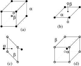
FIG. 1.: Definition of the duality operator $\ast^{K}\;$: $\alpha$ is a $p$-cell in $K$ and $\beta\!=\!\ast^{K}\alpha$ is the dual $(3\!-\!p)$-cell in $\widehat{K}$. (In (a) $\beta$ is the point (vertex in $\widehat{K}$) at the centre of the 3-cell $\alpha\,$, while in (d) $\beta$ is the 3-cell in $\widehat{K}$ which has the point $\alpha$ at its centre.)

FIG. 2.: $\gamma_{K}$ is the boundary of the surface $D_{K}$ made up of 2-cells of $K$. The vertical line segments are the duals of the 2-cells making up $D_{K}$.

REFERENCES

[1]
A. S. Schwarz, Lett. Math. Phys. 2, 247 (1978).
[2]
S. Deser, R. Jackiw, and S. Templeton, Phys. Rev. Lett. 48, 975 (1983);
Ann. Phys. (N.Y.) 140, 372 (1982).
[3]
E. Witten, Commun. Math. Phys. 121, 351 (1989).
[4]
M. Blau and G. Thompson, Ann. Phys. (N.Y.) 205, 130 (1991).
[5]
F. Wilczek, Phys. Rev. Lett. 48, 1144 (1982); Phys. Rev. Lett.
49, 957 (1982); Fractional Statistics and Anyon Superconductivity
(World Scientific, Singapore, 1990).
[6]
A. M. Polyakov, Mod. Phys. Lett. A3, 325 (1988);
S. Bahcall and L. Susskind, Int. J. Mod. Phys. B5, 2735 (1991).
[7]
D. H. Adams, Preprint in preparation.
[8]
D. H. Adams and S. Sen, Phys. Lett. B 353, 495 (1995).
[9]
D. B. Ray and I. M. Singer, Adv. Math. 7, 145 (1971); Proceedings
of Symposia in Pure Mathematics, Vol. 23, p. 167
(American Mathematical Society, 1973).
[10]
P. Becher and H. Joos, Z. Phys. C 15, 343 (1982).
[11]
A. R. Kavalov and R. L. Mkrtchian, Phys. Lett. B 242, 429 (1990);
Int. J. Mod. Phys. A 6 3919 (1991).
[12]
J. Cheeger, Ann. Math. 109, 259 (1979); W. Müller, Adv. Math.
28, 233 (1978).
[13]
Y. Takahashi and H. Umezawa, Collective Phenomena 1975 (Gordon and
Breach Scientific Publishers Ltd, 1975), Vol. 2, p. 55.
Reprinted in Int. J. Mod. Phys. B 10, 1755 (1996).
[14]
M. Creutz, Quarks, Gluons and Lattices (Cambridge Univ. Press,
Cambridge, 1983).
[15]
M. Creutz and M. Tytgat, Phys. Rev. Lett. 76, 4671 (1996).