IASSNS-HEP 97/28

SLAC-PUB-7468

SNUTP 97-043

SU-ITP 97/13

hep-th/9704142

CRITICAL POINTS AND PHASE TRANSITIONS

IN 5D COMPACTIFICATIONS OF M-THEORY
Aaron Chou^a, R. Kallosh^b, J. Rahmfeld^b,
Soo-Jong Rey ^abcd, M. Shmakova^be, Wing Kai Wong<sup>b

a</sup>Stanford Linear Accelerator Center, Stanford University, Stanford, CA 94309
^bPhysics Department, Stanford University, Stanford, CA 94305-4060
^cSchool of Natural Sciences, Institute for Advanced Study, Princeton, NJ 08540
^dPhysics Department, Seoul National University, Seoul 151-742 KOREA
^eUniversity of Tennessee, Knoxville, TN 37996

We study critical points of the BPS mass $Z$, the BPS string tension $Z_{m}$, the black hole potential $V$ and the gauged central charge potential $P$ for M-theory compactified on Calabi-Yau three-folds. We first show that the stabilization equations for $Z$ (determining the black hole entropy) take an extremely simple form in five dimensions as opposed to four dimensions. The stabilization equations for $Z_{m}$ are also very simple and determine the size of the infinite $adS_{3}$-throat of the string. The black hole potential in general exhibits two classes of critical points: supersymmetric critical points which coincide with those of the central charge and non-supersymmetric critical points. We then generalize the discussion to the entire extended Kähler cone encompassing topologically different but birationally equivalent Calabi-Yau three-folds that are connected via flop transitions. We examine behavior of the four potentials to probe the nature of these phase transitions. We find that $V$ and $P$ are continuous but not smooth across the flop transition, while $Z$ and its first two derivatives, as well as $Z_{m}$ and its first derivative, are continuous. This in turn implies that supersymmetric stabilization of $Z$ and $Z_{m}$ for a given configuration takes place in at most one point throughout the entire extended Kähler cone. The corresponding black holes (or string states) interpolate between different Calabi-Yau three-folds. At the boundaries of the extended Kähler cone we observe that electric states become massless and/or magnetic strings become tensionless.

1 Introduction

In the moduli space encompassing all known perturbative string theories, it has been discovered [1] that there exists a special point at which perturbative string theories are strongly coupled and are best described by a more fundamental eleven-dimensional theory. For low-energy excitations, this so-called M-theory is given by eleven-dimensional $N=1$ supergravity [2] appended with gravitational anomaly cancellation terms. Not only providing a more fundamental description of non-perturbative string theories, M-theory is also indispensable for constructing a phenomenologically viable four-dimensional string compactifications. Witten [3] has shown that strongly coupled phase of $E_{8}\times E_{8}$ heterotic string theory, which is most appropriately described by M-theory compactified on an orbifold ${\bf S}_{1}/{\bf Z}_{2}$, is crucial for unification of all gauge and gravitational couplings at the grand-unification scale .

The above consideration points to the importance of a better understanding of M-theory compactification vacua. With such motivation, in the present paper, we study M-theory compactified on Calabi-Yau three-folds $CY_{3}$ to five dimensions. The compactification appropriately encodes the strong coupling limit of type IIA compactification on the same Calabi-Yau three-fold $CY_{3}$. After the compactification, the low-energy dynamics is governed by a $d=5,N=2$ supergravity. Its field content and interactions are determined by the topological data of $CY_{3}$, which may be understood, for example, from eleven-dimensional supergravity compactified on $CY_{3}$[5, 6].

In understanding the web of moduli spaces of string compactification vacua, it has become clear that two aspects are essential. First, the classical moduli space may undergo topology changing phase transitions accompanied by the appearance of massless states. Resolution of conifold singularities [7], symmetry enhancement by small instantons [8] and the appearance of tensionless strings [9, 10, 11, 12, 13] are well-known instances. At the same time, it has become clearer that BPS black holes with finite horizon serve as a spacetime probe of the compactified internal space [14, 16, 17, 18, 19, 20, 21]. For example, for $d=4,N=2$ supergravity theory, the so-called doubly extreme black holes attract Kähler moduli scalar fields to a critical point of the central charge, $\partial Z/\partial\phi^{i}=0$. The extremized BPS black hole mass then becomes equal to the square root of the entropy, and depends only on topological data of the compactified space such as intersection numbers, the second Chern class and rational, elliptic instanton numbers.

In five dimensions, Witten [22] has shown that all phases of the M-theory compactification vacua are purely geometrical. Since the Kähler moduli do not admit complexificiation in five dimensions, the topology changing phase transitions in five dimensions are sharp. As such, the nature of phase transitions is quite distinct from that in four dimensions. It is therefore of interest to understand all distinct features of the phase transition explicitly by means of simple probes. As in thermodynamical systems, the nature of phase transitions and the corresponding critical behavior can be probed by various supersymmetry potentials of Landau-Ginzburg type. The BPS central charge $Z$, defined as the electric charge of the gravi-photon, which is the BPS mass of the electric 5d black holes, is one of such potentials. Similarly, the magnetic charge of the gravi-photon $Z_{m}$ defines the tension of the magnetic 5d string and also can be used to probe the phase transition. Likewise, the black hole potential $V$ and the gauged central charge potential $P$ are other additional physical quantities that can be used for analyzing the topology-changing phase transitions. All these potentials are defined for fixed electric charges (wrapping numbers of M-branes on two-cycles of the Calabi-Yau three-fold) and may be regarded as independent thermodynamic potentials in the canonical ensemble. The critical point in the vector moduli space is determined entirely by the chosen charge configuration for the potentials. The idea is that, by considering different charge configurations, the critical configuration of the Kähler moduli for each of the above physical quantities may be located at different phases of the Calabi-Yau three-fold, hence, probing the nature of phase transitions.

This paper is organized as follows. In section 2 we review the compactification of M-theory on a Calabi-Yau threefold. The resulting low-energy approximation, $d=5,N=2$ supergravity coupled to abelian vector supermultiplets, is based on the structure of very special geometry [24]. In section 3, we derive the stabilization equations of five-dimensional vector moduli scalars for electrically charged particle states and magnetic string states. The central charge $Z$ evaluated at these fixed scalar field values turns out to be a minimum as expected. In section 4, we introduce two five-dimensional potentials of interest :– the black hole potential $V$ and the scalar potential $P$ which arises in gauged supergravities. The central charge $Z$ and these two potentials are explicitly discussed in a simple example. Section 5 constitutes the main results of our study. After reviewing briefly some basic notions of the five-dimensional extended Kähler cone, we probe the topology-changing phase transitions using the supersymmetry potentials $Z$, $Z_{m}$, $V$ and $P$. Particular emphasis is put on flop transitions connecting two adjacent Kähler cones. We analyze how $Z$, $V$ and $P$ are affected by it. We find that the electric central charge and its first two derivatives are in fact continuous along the flop transition. Since, as we will also show, any extremum of $Z$ has to be a minimum one finds uniqueness of the critical point of $Z$ in the entire extended Kähler cone. Whereas the magnetic central charge (BPS tension) and its first derivative are continuous, also implying uniqueness of the stabilization point in the extended Kähler cone, $V$ on the other hand shows a kink at the flop transition. Before we conclude, our results are verified by an explicit example in section 6, where we study one particular extended Kähler cone in detail. The behavior of the potentials is graphically displayed. In addition we find new critical points for the potentials $V$ and $P$. We observe that extremal transitions in five dimensions between Calabi-Yau spaces with different numbers of Kähler moduli often involve tensionless strings.

2 Very Special Geometry and Calabi-Yau Manifolds

We begin by recalling relevant aspects [5, 25] of M-theory compactification on a Calabi-Yau three-fold $CY_{3}$ with Hodge numbers $h_{(1,1)}$, $h_{(2,1)}$ and intersection numbers $C_{IJK}(I,J,K=1,\cdots,h_{(1,1)})$. The bosonic fields of the supergravity multiplet in eleven dimensions consist of the metric $g_{MN}$ and the 3-form antisymmetric tensor potential ${\cal A_{MNP}}$. Denote the complex coordinates of $CY_{3}$ as ${\cal I},{\cal J},{\overline{\cal I}},{\overline{\cal J}}=1,2,3$. After compactification on the $CY_{3}$, the action contains one CY complex axion ${\cal A}_{{\cal IJK}}=\epsilon_{\cal IJK}b$, one universal axion $a\,\,(da\sim{}^{*}d{\cal A})$, the Calabi-Yau volume ${\rm det}~{}{\cal G_{I{\overline{J}}}}$, $h_{(1,1)}-1$ real Kähler moduli ${\cal G_{I{\overline{J}}}}$ and $h_{(2,1)}$ pairs of complex scalars $({\cal G_{IJ}},{\cal A_{IJ{\overline{K}}}})$. In addition, $h_{(1,1)}$ abelian vector potentials ${\cal A}_{\mu{\cal I{\overline{J}}}}$ arise, one of which becomes the gravi-photon. They combine into $d=5$ supermultiplets as follows. Taking into account one graviphoton in the supergravity multiplet, there are $h_{(1,1)}-1$ vector multiplets consisting of uni-modular $({\cal G_{I{\overline{J}}}},{\cal A}_{\mu{\cal I{\overline{J}}}})$, one universal hypermultiplet $({\rm det}~{}{\cal G_{I{\overline{J}}}},a,{\cal A_{IJK}})$, and $h_{(2,1)}$ hypermultiplets containing $({\cal G_{IJ}},{\cal A_{IJ{\overline{K}}}})$. Supersymmetry non-renormalization theorems [26, 27] ensure that the moduli space of the hypermultiplets containing the complex structure moduli (and the size of the entire Calabi-Yau space) is completely disconnected from the Kähler moduli space.

In this paper we will restrict ourselves to the moduli space of the vector multiplets, corresponding to the Kähler moduli $t^{I}$ of the Calabi-Yau space. The Kähler moduli are derived from the Kähler form $J$ on $CY_{3}$ by expanding into a fundamental 2-form basis $J_{I}$ as

$$J=t^{I}J_{I}.$$ (2.1)

With this definition the moduli $t^{I}$ correspond to the sizes of 2-cycles in $CY_{3}$ dual to the $J_{I}$.

The supersymmetric coupling of $d=5,N=2$ vector multiplets to N=2 supergravity has been constructed in [28]. The vector multiplet coupling is determined completely by specifying a prepotential

$${\cal V}=C_{IJK}t^{I}t^{J}t^{K},\hskip 28.45274ptI=(1,\cdots,h_{(1,1)}),$$ (2.2)

which defines intrinsic ‘very special geometry’ [24]. The prepotential is related to the overall volume of Calabi-Yau three-fold. In five dimensions, the overall volume belongs to the so-called universal hypermultiplet. Therefore, the prepotential which encodes independent degrees of freedom of the vector multiplet moduli space is constrained to satisfy

$${\cal V}=1.$$ (2.3)

The variables $t^{I}$ are related to the conventional very special coordinates [29] $X^{I}$ by the rescaling

$$t^{I}=6^{\frac{1}{3}}X^{I}.$$ (2.4)

The $h_{(1,1)}-1$ independent, real scalar fields parametrizing the vector multiplet moduli space are denoted by $\phi^{i}$, and the $t^{I}$ are functions of them. It is often convenient to identify the $\phi^{i}$ with $h_{(1,1)}-1$ of the $t^{I}$ and to take the remaining Kähler moduli to be a function of the other ones defined by the constraint ${\cal V}=1$.

In terms of the aforementioned normalization convention, the bosonic part of the action is given by

$$e^{-1}{\cal L}=-{1\over 2}R-{1\over 4}G_{IJ}(\phi)F_{\mu\nu}{}^{I}F^{\mu\nu J}-{1\over 2}g_{ij}(\phi)\partial_{\mu}\phi^{i}\partial^{\mu}\phi^{j}+{e^{-1}\over 48}\epsilon^{\mu\nu\rho\sigma\lambda}C_{IJK}F_{\mu\nu}^{I}F_{\rho\sigma}^{J}A_{\lambda}^{K}.$$ (2.5)

The vector multiplet coupling is defined by

$$G_{IJ}=-\frac{1}{2\cdot 6^{\frac{2}{3}}}\partial_{I}\partial_{J}(\ln{\cal V})|_{{\cal V}=1},$$ (2.6)

while the moduli space metric $g_{ij}$ is given by

$$g_{ij}=6^{\frac{2}{3}}G_{IJ}t^{I}_{,i}t^{J}_{,j}=-3C_{IJK}t^{I}t^{J}_{,i}t^{K}_{,j}.$$ (2.7)

The scalar fields $\phi^{i},\,\,(i=1,\cdots,h_{(1,1)}-1)$ parametrize the vector multiplet moduli space ${\cal M}_{V}$. For a given ${\cal M}_{V}$, consider the second covariant derivative of the very special coordinate with respect to the moduli scalar fields $\phi^{i}$

$$(t^{I})_{,i;j}=(2/3)g_{ij}t^{I}-\sqrt{2/3}\;T_{ijk}t^{I,k}.$$ (2.8)

The symmetric tensor $T_{ijk}$, which is a function of the moduli scalar fields, encodes local geometric structures of ${\cal M}_{V}$. If $T_{ijk}$ is covariantly constant, $T_{ijk;l}=0$, the scalar manifold ${\cal M}_{V}$ is locally a symmetric space. $d=5,N=2$ supergravity with locally symmetric ${\cal M}_{V}$ has been studied extensively with the aid of Jordan algebras [28]. Generically, with $n\equiv h_{(1,1)}-1$,

$${\cal M}={SO(1,1)}\times{SO(1,n-1)\over SO(n-1)}.$$ (2.9)

In this case the prepotential ${\cal V}=C_{IJK}t^{I}t^{J}t^{K}$ should be factorizable into a linear and a quadratic polynomial parts. That is,

$${\cal V}=C_{IJK}t^{I}t^{J}t^{K}=t^{1}Q(t^{\lambda})$$ (2.10)

where $\lambda=2,..,n$ and $Q$ is a quadratic form of signature $(+,-,-,\dots,-)$. If ${\cal V}$ is not factorizable, ${\cal M}_{V}$ may or may not be a symmetric space. The cases with locally symmetric and homogeneous manifold ${\cal M}_{V}$, but with non-factorizable prepotential ${\cal V}$ have been classified in [28]. There are only four exceptional cases, so-called ‘magic square’ supergravities, for which $n=3(1+{\rm dim}{\bf A})$ where ${\bf A}$ is one of the division algebras and $n=5,8,14,26$.

In generic Calabi-Yau compactifications of M-theory, the prepotentials do not belong to the set based on the Jordan algebra classification of $d=5$ supergravities. Possible exceptions are Calabi-Yau compactifications described by factorizable prepotentials of the form (2.10) or the ‘magic square’ cases $n=5,8,14,26$. In all other cases, the $d=5$ compactifications do not share many of the properties of the known $d=5$ supergravities based on the Jordan algebras. In following sections, we will study Calabi-Yau prepotentials with small dimensions of vector moduli spaces $n=1,2$, which are neither factorizable nor belong to the “magic square” cases. As we will see, these examples are simple enough to allow a detailed analysis, while rich enough to capture all the essentials of geometric phase transitions in five dimensions.

3 Stabilization Conditions

In $d=5,N=2$ supergravity theories, the gravi-photon field $T$ is given by a linear combination of all vector fields $F^{I}$ of the theory with moduli dependent coefficients: $T=t^{I}(\phi)G_{IJ}(\phi)F^{I}$. Associated to the gravi-photon is the electric central charge [25]

$$Z=t^{I}(\phi)q_{I}$$ (3.1)

where $q_{I}$ is the quantized electric charge for each vector field $G_{I}\equiv G_{IJ}F^{I}$. In the context of M-theory the electrically charged point-particle states are identified with BPS winding states of the M-theory membrane around 2-cycles of the Calabi-Yau three-fold $CY_{3}$ [5, 25, 27]. Magnetically charged string states are identified with BPS winding states of the M-theory five-brane around 4-cycles. The magnetic central charge describing the string tension is given by [25]

$$Z_{m}=t_{I}(\phi)m^{I}$$ (3.2)

where the dual moduli $t_{I}$ defined by

$$t_{I}=C_{IJK}t^{J}t^{K}$$ (3.3)

encode the sizes of four-cycles of the $CY_{3}$. The mass spectrum of BPS states varies over the vector multiplet moduli space. As such, the mass of a BPS state can often be extremized as a function of moduli for given values of charges $q_{I}$ [16, 15]. It is therefore of interest to study critical behavior of the BPS mass-squared over the moduli space ${\cal M}_{V}$

$$M^{2}_{\rm BPS}=Z^{2}(q_{I},C_{IJK},\phi^{i})=t^{I}t^{J}q_{I}q_{J}.$$ (3.4)

The critical points of the BPS mass-squared are specified by the extremal value of the central charge $\partial_{i}Z=0$ or by the vanishing of the central charge $Z=0$ since

$${\partial M^{2}_{\rm BPS}\over\partial\phi^{i}}=2Z\,\partial_{i}Z=2(t^{I})_{,i}\;q_{I}\;t^{J}q_{J}=0.$$ (3.5)

In the $d=4,N=2$ theory the extremal configuration of the central charge $\partial_{i}Z=0$ has been found to be a solution of a set of so-called stabilization equations, which define functional relations between microscopic charges and moduli scalar fields at the critical points [16, 15]. Quite often, the stabilization condition equations are easier to solve than the problem of extremizing directly the central charge [17, 18, 19, 20, 21].

In what follows, we derive the corresponding stabilization condition equations for $d=5,N=2$ supergravity in two alternative ways. The first derivation extends the method utilized in the $d=4,N=2$ context [16, 15]: the very special geometry that underlies the vector moduli space is used to invert the implicit functional relations $\partial_{i}Z=(t^{I})_{,i}q_{I}=0$ into equations between charges and moduli. The second method employs a Lagrange multiplier to the constraint equation ${\cal V}(t)=C_{IJK}t^{I}t^{J}t^{K}=1$ and also effectively inverts the $(t^{I})_{,i}q_{I}=0$ condition.

3.1 Stabilization of the Electric Central Charge: Very Special Geometry

To invert $\partial_{i}Z=(t^{I})_{,i}q_{I}=0$ and find the expression for $q_{I}$’s in terms of $t^{I}$’s we will utilize some of the properties of the very special geometry presented in [29]. We first multiply $\partial_{i}Z$ by $g^{ij}t^{J}{}_{,j}$ and get

$$\partial_{i}Z=(t^{I})_{,i}q_{I}=0\qquad\Longrightarrow\qquad g^{ij}t^{I}{}_{,i}t^{J}{}_{,j}\,q_{I}\equiv\Pi^{IJ}q_{I}=-{1\over 3}((C^{IJ}-t^{I}t^{J})q_{I}=0$$ (3.6)

where the matrix $C^{IJ}$ is the inverse matrix of $C_{IJ}=C_{IJK}t^{K}$. Multiplying this equation by $C_{KJ}$, we find that

$$q_{K}=C_{KJ}t^{J}Z=C_{IJK}t^{J}t^{K}Z$$ (3.7)

at $\partial_{i}Z=0$. Thus the $d=5$ stabilization condition equations have a particularly simple form

$$q_{I}=Zt_{I}$$ (3.8)

where $t_{I}$, as defined in (3.3), is the coordinate dual to the very special coordinate $t^{I}$.

3.2 Alternative Derivation: Lagrange Multiplier Method

We use the linear sigma model approach to the constraint of the prepotential. Consider a function:

$$\tilde{Z}(t^{I})=Z+\lambda({\cal V}-1)=q_{I}t^{I}+\lambda(C_{IJK}t^{I}t^{J}t^{K}-1),$$ (3.9)

where the $t^{I}$’s are a priori unconstrained and $\lambda$ denotes a Lagrange multiplier. Taking derivatives with respect to $t^{I}$ we obtain a set of extremization equations:

$$q_{I}+3\lambda C_{IJK}t^{J}t^{K}=0.$$ (3.10)

Similarly, the extremization condition with respect to $\lambda$ gives:

$$C_{IJK}t^{I}t^{J}t^{K}=1.$$ (3.11)

Contracting (3.10) with $t^{I}$ and using the constraint (3.11) we solve for $\lambda$ as

$$3\lambda=-q_{I}t^{I}=-Z.$$ (3.12)

Substituting (3.11) into (3.10) we obtain

$$q_{I}-ZC_{IJK}t^{J}t^{K}=0.$$ (3.13)

In terms of the dual variable $t_{I}$, the solution is

$$q_{I}=Zt_{I},$$ (3.14)

yielding the same result as the very special geometry method.

For later use, we find it useful to put the $d=5$ stabilization equation with a suitable rescaling. Let us call $\bar{t}^{I}$ the original very special coordinate rescaled by the square root of the central charge

$$\bar{t}^{I}\equiv\sqrt{Z}\;t^{I}.$$ (3.15)

Since the coordinates $t^{I}$ of the very special geometry are real, the rescaled coordinates $\bar{t}^{I}$ have to be real for configurations with positive value of the central charge. In $d=5$, one can also consider the case of imaginary $\bar{t}$ with negative $Z$. One can see however that this case is easily reproduced starting with the configuration with positive $Z$ and real solutions for $\bar{t}$ by flipping the signs of all charges, as the critical points of $Z$ and $-Z$ do coincide manifestly. It is then possible to rewrite the $d=5$ stabilization equation into a rather suggestive form

$$q_{I}=C_{IJK}\bar{t}^{J}\bar{t}^{K}.$$ (3.16)

This equation implies that, for a given choice of Calabi-Yau manifold with specific topological intersection numbers and a given number of moduli fields, the value of the electric charge $q_{I}$ defines the real (imaginary) values of rescaled moduli via eq.(3.16), which is quadratic in the rescaled moduli. The solution may or may not exist for the real (or purely imaginary) $\bar{t}^{I}$. In cases where the solution exists we have an explicit expression for the extremum of the BPS mass and for the black hole entropy. Once the solution to eq. (3.16) is found in the form $\bar{t}^{I}(q_{L},C_{IJK})$ we find the critical value of the central charge in the form

$$\left(\bar{t}^{I}q_{I}\right)^{2}=Z^{3}_{\rm cr}(q_{L},C_{IJK}).$$ (3.17)

This in turn defines the entropy of the black hole [16, 15, 29]

$$S(q_{L},C_{IJK})={\pi^{2}\over 12}|Z_{\rm cr}|^{3/2}.$$ (3.18)

Recall that the near horizon geometry of the $d=5$ black hole is given by $adS_{2}\times S^{3}$, hence, the black hole entropy is proportional to the volume of the $S^{3}$. The expression for the critical value of the central charge has been found previously [16, 15, 29] in the form $(Z)^{2}_{\rm cr}=q_{I}q_{J}(C^{IJ})_{\rm cr}$. The new $d=5$ stabilization equation (3.16) enables to find the entropy of $d=5$ black holes explicitly as a function of the microscopic electric charges and of the CY topological intersection numbers.

Indeed, the structure of the $d=5$ stabilization equations are far simpler to solve than those in the $d=4$ case. In [30] it was found that the $d=4,N=2$ black hole entropy with classical Calabi-Yau prepotential can be understood completely once a real solution is found to the following set of algebraic equations: $\Delta_{I}=C_{IJK}\tilde{x}^{J}\tilde{x}^{K}$ where $\Delta_{I}$ is some particular combination of microscopic electric and magnetic charges and topological intersection numbers. When these equations have a solution with real $\tilde{x}^{J}$, an algorithm was presented for finding the fixed values of moduli, the central charge and the entropy of black holes. The algorithm was general enough but the explicit form of the result was rather complicated.

In $d=5$ the situation has been simplified considerably. The stabilization equations $q_{I}=C_{IJK}\bar{t}^{J}\bar{t}^{K}$ coincide with the algebraic equations of [30] $\Delta_{I}=C_{IJK}\tilde{x}^{J}\tilde{x}^{K}$ upon identification $\Delta_{I}\sim q_{I}$ and $\bar{t}^{J}\sim\tilde{x}^{J}$. Moreover, the algorithm for obtaining the critical value of the BPS mass and the entropy after $\bar{t}$ is found is very simple in $d=5$ and displayed in eqs. (3.17 ) and (3.18). If one would like to use the critical value of the $d=4$ central charge directly to find the critical value of its 5d counterpart the following restrictions have to be applied to the $d=4$ charges: $p^{I}=q_{0}=p^{0}-1=0$.

3.3 Stabilization of the Magnetic String Tension

The magnetic central charge determining the tension of the magnetic string states [25] is a function of the moduli as well, hence, one can also have a critical point for fixed values of the microscopic magnetic charges $m^{I}$

$$\partial_{i}Z_{m}=(t_{I})_{,i}m^{I}=2C_{IJK}t^{I}(t^{J})_{,i}m^{K}=0.$$ (3.19)

To invert this relation we proceed similarly as before

$$C_{IJK}t^{I}(t^{J})_{,i}(t^{L})_{,j}g^{ij}m^{K}=C_{IJK}t^{I}m^{K}(C^{JL}-t^{J}t^{L})=0.$$ (3.20)

It follows that

$$m^{L}=t^{L}Z_{m}\qquad\Rightarrow\qquad t^{L}={m^{L}\over Z_{m}}.$$ (3.21)

The critical value of the dual coordinate is

$$t_{I}={C_{IJK}m^{J}m^{K}\over Z^{2}_{m}}$$ (3.22)

and the critical value of the BPS string tension is

$$(Z_{m})^{3}_{\rm cr}=(t_{L}m^{L})^{3}_{\rm cr}=C_{IJK}m^{I}m^{J}m^{K}.$$ (3.23)

For the electrically charged $d=5$ BPS black holes, the critical value of the BPS mass was related to the horizon volume $S^{3}$, where the near horizon geometry was given by $adS_{2}\times S^{3}$. This in turn was proportional to the black hole entropy. For the magnetically charged $d=5$ BPS black string, we find similarly that the extremized value of the BPS tension is related to the volume of the $S^{2}$ as well as to the size of the infinite throat of $adS_{3}$ where the near horizon geometry is given by $adS_{3}\times S^{2}$. The volume of $S^{2}$ is moduli independent and is proportional to $Z_{m}^{2}=(C_{IJK}m^{I}m^{J}m^{K})^{2\over 3}$. For $d=4$ black holes the relevant no-axion black hole solution with the entropy proportional to $\sqrt{q_{0}C_{IJK}m^{I}m^{J}m^{K}}$ was found in [19] and an empirical rule of state counting in M-theory was proposed in [31], [32] to explain the entropy. Upon decompactification to $d=5$ this black hole solution was identified with the magnetic string in [33]. Here we have found that the stabilization of the magnetic string tension in $d=5$ describes the same structure as the stabilization of the magnetic no-axion black hole in $d=4$ with unit electric charge $q_{0}=1$. The critical value of the 5d magnetic tension can be obtained from the stabilization of the 4d black hole mass at $q_{0}-1=q_{I}=p^{0}=0$. This result follows simply from comparing $d=4$ results for the black hole with the $d=5$ results for the magnetic string.

3.4 The Extremum of the BPS Mass is a Minimum

A natural question to address is under what conditions the extremum of the BPS mass is a minimum. An analogous issue has been already addressed in the context of $d=4$ special geometry [34], where it was found that

$$D_{i}D_{j}Z^{2}=\frac{1}{2}g_{ij}Z^{2}\qquad{\rm at}\qquad\partial_{i}Z=0.$$ (3.24)

In $d=5$ the corresponding calculation yields, using eq. (2.8):

$$D_{i}D_{j}Z=\partial_{i}\partial_{j}Z={2\over 3}g_{ij}Z_{\rm cr}\qquad{\rm at}\quad\partial_{i}Z=0\ .$$ (3.25)

This shows that the extremum of the central charge is a minimum (maximum) if the central charge at the critical point is positive (negative), using the fact that the metric of the moduli space is positive definite. For the square of the BPS mass we get

$$D_{i}D_{j}(Z)^{2}=\partial_{i}\partial_{j}(Z)^{2}={4\over 3}g_{ij}(Z^{2})_{\rm cr}\qquad{\rm at}\quad\partial_{i}Z=0\ .$$ (3.26)

The same is true for the magnetic BPS mass. Thus, as long as the very special geometry is regular viz. $g_{ij}$ and $G_{IJ}$ are positive definite and non-degenerate, the BPS mass has a minimum at the critical point. Hence, for a given choice of charges and signs of moduli at infinity the corresponding minimum, if it exists, is unique.

4 The Black Hole and Gauged Central Charge Potentials

In the last section we have studied the critical points of the central charge $Z$ in detail. For black holes, a quantity of more direct significance is the black hole potential $V$. In this section we introduce this potential along with a gauged central charge potential $P$, which arises in gauged supergravities, and discuss their respective critical points in detail. We will also compare the critical behavior of $Z^{2}$, $V$ and $P$ for an example defined by prepotential ${\cal V}=STU$.

4.1 The Black Hole Potential and Its Critical Points

In the context of $d=4,N=2$ supergravity, it was explained in [34] that the stabilization of moduli fields of BPS black holes near the black hole horizon depends on the properties of the so-called black hole potential $V$. For extremal (but not necessarily supersymmetric) black holes with regular horizon and regular moduli scalars, the following relations have been established. The entropy is defined (in eq. (26) of [34]) as the value of the black hole potential evaluated at the horizon:

$${S\over\pi}=V(p,q,\phi_{h}).$$ (4.1)

Furthermore, in [35, 34, 36], it was found that the ADM mass of a generic non-extreme black hole consists of three contributions: the black hole potential depending on the value of moduli at infinity, some function of the scalar charges and the $(2ST)^{2}$ term, where $T$ is the black hole temperature:

$$(M_{\rm ADM})^{2}=V(p,q,\phi_{\infty})-G_{ab}\Sigma^{a}\Sigma^{b}+(2ST)^{2}.$$ (4.2)

For the case of $d=4,N=2$ supergravity, utilizing special geometry relations, $V$ was found to be equal to $|Z|^{2}+|\partial Z|^{2}$. In the extreme case when $TS=0$ there are two possibilities: (1) the extreme black hole is supersymmetric

$$(M_{\rm ADM})^{2}=(M_{\rm BPS})^{2}=|Z(p,q,\phi_{\infty})|^{2},$$ (4.3)

which requires for consistency that $|\partial Z(p,q,\phi_{\infty})|^{2}=G_{ab}\Sigma^{a}\Sigma^{b}$ and the entropy is given by ${S\over\pi}=V(p,q,\phi_{h})=|Z|^{2}$ at $\partial_{i}|Z|=0$, or (2) the extreme black hole is not supersymmetric

$$(M_{\rm ADM})^{2}=|Z|^{2}+|\partial Z|^{2}-G_{ab}\Sigma^{a}\Sigma^{b}>|Z(p,q,\phi_{\infty})|^{2}=(M_{\rm BPS})^{2}$$ (4.4)

and the black hole horizon area is still given by the value of the potential at the horizon ${S\over\pi}=V(p,q,\phi_{h})$ if the moduli are regular (in such cases the critical point of the black hole potential is not defined by the enhancement of unbroken supersymmetry ($\partial_{i}|Z|=0$) as it happens for supersymmetric black holes). The potential has a critical point which describes the stabilization of moduli near the horizon of extreme non-supersymmetric black holes. These non-supersymmetric critical points have not been studied much previously. However, the extreme non-supersymmetric solutions with (or without) regular horizon have been known to exist [37, 38, 39, 40]. The most recent detailed study of such solutions in $N=4$ and $N=8$ supergravity theories was given in [41].

In what follows we will study the analogous black hole potential in $d=5$. We will find as expected both types of critical points. The gauge kinetic term in the Lagrangian responsible for the black hole potential is proportional to $G_{IJ}F^{I}F^{J}$. Using eqs. (16,29) from [29] one finds that the $d=5$ potential whose critical points describe the BPS mass and the stabilization of moduli for extreme black holes is given by

$$V=Z^{2}+{3\over 2}g^{ij}\partial_{i}Z\partial_{j}Z=\left(t^{I}t^{J}+{3\over 2}g^{ij}(t^{I})_{,i}(t^{J})_{,j}\right)q_{I}q_{J}.$$ (4.5)

It can be shown that the potential is proportional to the gauge couplings

$$V={6^{1/3}\over 4}G^{IJ}(\phi)q_{I}q_{J}$$ (4.6)

and the critical points of this potential are given by

$$\partial_{i}V=4\partial_{i}ZZ-\sqrt{6}\;T_{ikj}\partial^{k}Z\partial^{j}Z=0.$$ (4.7)

There can be

1. Supersymmetric critical points. Obviously the critical point of the central charge is also a critical point of the potential

$$\partial_{i}V=0\qquad{\rm at}\quad\partial_{i}Z=0.$$ (4.8)

This applies to supersymmetric extreme black holes. The inverse is not true: it is possible that there is a

2. Non-supersymmetric critical point where

$$\partial_{i}V=0\qquad{\rm at}\quad\partial_{i}Z\neq 0$$ (4.9)

which give rise to stabilization of the moduli also for non-supersymmetric black holes. The calculation of the second derivative of the potential at the supersymmetric critical point is straightforward and is given by

$$(V)_{,i;j}=\partial_{i}\partial_{i}V={8\over 3}g_{ij}V_{\rm cr}\qquad{\rm at}\qquad\partial_{i}V=\partial_{i}Z=0.$$ (4.10)

We conclude that for a positive definite metric of very special geometry the potential has a minimum at the supersymmetric critical point (4.8), which exists under the condition that the stabilization equation (3.16) for the moduli in terms of charges has a real solution.

The non-supersymmetric critical points (4.9) do not seem to allow a simple general treatment. We will study them for a few examples and show that indeed such critical points do exist.

4.2 The Gauged Central Charge Potential

The gauged central charge of $N=2$ supergravity arises in theories in which an $U(1)$ subgroup of the $SU(2)$ automorphism group of the $N=2$ supersymmetry algebra is gauged [28]. The gauging which breaks $SU(2)$ down to $U(1)$ is realized by making the gravitino and gaugino charged so that their covariant derivatives are

$$(D_{\mu}\lambda^{i})^{\alpha} = \nabla_{\mu}\lambda^{i^{\alpha}}+gV_{I}A_{\mu}{}^{I}\delta^{\alpha\beta}\lambda^{i}{}_{\beta}$$ (4.11)

$$(D_{\mu}\psi_{\nu})^{\alpha} = \nabla_{\mu}\psi_{\nu}^{\alpha}+gV_{I}A_{\mu}{}^{I}\delta^{\alpha\beta}\psi_{\nu}{}_{\beta}\ ,\qquad\alpha,\beta=1,2.$$ (4.12)

To maintain the $N=2$ supersymmetry intact after the gauging, one has to add to the theory the gauged central charge potential proportional to $g^{2}P$, where

$$P=Z^{2}-{3\over 4}g^{ij}\partial_{i}Z\partial_{j}Z.$$ (4.13)

In the context of gauged supergravity the central charge is actually a moduli dependent combination of gravitino and gaugino charges defined by

$$Z=t^{I}V_{I}$$ (4.14)

where $V_{I}$ is the charge defining the gravitino-gravitino-vector and gaugino-gaugino-vector interactions as may be deduced from their respective covariant derivatives. In addition to the potential, there are gravitino and gaugino mass terms proportional to

$$L_{\rm mass}^{\rm grav} = -i\bar{\psi}^{\alpha}_{\mu}\Gamma^{\mu\nu}\psi^{\beta}_{\nu}\delta_{\alpha\beta}Z$$ (4.15)

$$L_{\rm mass}^{\rm gauge} = -i\bar{\lambda}^{\alpha i}\lambda^{\beta j}\delta_{\alpha\beta}\left(g_{ij}Z+4\sqrt{2}T_{ijk}Z^{,k}\right)$$ (4.16)

and a mixing term proportional to the derivative of the central charge $\bar{\lambda}^{\alpha i}\Gamma^{\nu}\psi^{\beta}_{\nu}\delta_{\alpha\beta}Z_{,i}$. Thus in this theory the masses of gravitino and gaugino coincide with the BPS mass in the generic point of the moduli space up to terms proportional to the derivative of the central charge in the moduli space. This observation implies that at supersymmetric critical points where $Z_{,i}=0$, one finds

$$M^{\rm grav}=M^{\rm gauge}=|(t^{I})_{\rm cr}V_{I}|=|Z_{\rm cr}(V_{I},C_{IJK})|\qquad{\rm at}\qquad Z_{,i}=0.$$ (4.17)

It is interesting to note that, as a function of gravitino charges and topological intersection numbers, the gravitino mass is given by the same topological formula which defines the entropy of the extreme supersymmetric black holes as function of black hole charges. The critical points of the $P$ are given by

$$\partial_{i}P=Z\,\partial_{i}Z+\sqrt{3/2}\;T_{ijk}\partial^{j}Z\partial^{k}Z=0.$$ (4.18)

As in previous cases it is straightforward to study supersymmetric critical point where the second derivative of the potential is proportional to the metric on the moduli space:

$$(P)_{,i;j}=\partial_{i}\partial_{i}P={2\over 3}g_{ij}(Z^{2})_{\rm cr}\qquad{\rm at}\qquad\partial_{i}P=\partial_{i}Z=0.$$ (4.19)

Within the validity range of very special geometry, this potential has a minimum whenever the stabilization equation has a solution. In the case of potentials related to Jordan algebras all critical points of $P$ have been classified in [28], where two types of critical points were described. It was found that the first derivative of the potential vanishes when the configuration of charges is such that either the derivative of the central charge is vanishing in our formalism or the potential is vanishing

$$\partial_{i}P\sim\partial_{i}Z\>P=0\qquad{\rm at}\qquad\partial_{i}Z=0\quad{\rm or}\qquad P=0.$$ (4.20)

In the first case, the potential is non-zero at the minimum giving rise to a cosmological constant. This critical point is associated with supersymmetric black holes and extremization of their mass. The second case with the identically vanishing potential (cosmological constant) is specific to the theories associated with irreducible idempotents of the Jordan algebra.

As explained in section 2, M-theory compactified on a $CY_{3}$ manifold typically does not give rise to a factorizable prepotential nor corresponds to one of the magic square supergravity theories. Properties of the supersymmetric critical points of $V$ and $P$ can be studied using eqs. (4.8,4.19). However, critical points of any other nature are neither known nor excluded for the two potentials in case generic $CY_{3}$ compactifications. We will see however in section 6 by analyzing specific examples that generically there exist additional critical points.

To become familiar with the various kinds of potentials discussed so far we will examine a simple example defined by ${\cal V}=STU$. Although this prepotential does not directly correspond to a Calabi-Yau compactification it is useful enough to illustrate some essential ideas.

4.3 The ${\cal V}=STU=1$ Example

This example corresponds to a factorizable case, hence, the full Jordan algebra apparatus applies and in fact this prepotential has been studied in detail in [28]. The solutions to the stabilization equations are given by

$$S = (\frac{q_{T}q_{U}}{q_{S}^{2}})^{\frac{1}{3}}$$

$$T = (\frac{q_{U}q_{S}}{q_{T}^{2}})^{\frac{1}{3}}$$ (4.21)

$$U = (\frac{q_{S}q_{T}}{q_{U}^{2}})^{\frac{1}{3}}$$

and lead to the central charge

$$Z=3(q_{S}q_{T}q_{U})^{\frac{1}{3}}.$$ (4.22)

At this point we have not explicitly required positivity of the moduli fields. The result (4.21) shows that we find exactly one critical point of the central charge for a given set of charges. However, only if all of them are positive corresponding to no anti-brane configurations, we find the stabilization of the central charge for positive values of the moduli fields.

To understand the structure of the moduli space it is also instructive to analyze the moduli space metric $g_{ij}$ and the gauge couplings $G_{IJ}$. Taking $S$ as the dependent field, we find

$$g_{(TU)} = \pmatrix{\frac{1}{T^{2}}&\frac{1}{2TU}\cr\frac{1}{2TU}&\frac{1}{U^{2}}\cr}$$

$$G = \frac{1}{2\times 6^{\frac{2}{3}}}\pmatrix{\frac{1}{T^{2}}&0&0\cr 0&\frac{1}{U^{2}}&0\cr 0&0&T^{2}U^{2}\cr}.$$ (4.23)

Clearly, whenever either of the boundaries $T=0$ or $U=0$ is approached the corresponding matrix elements in $g$ and $G$ diverge. This implies that the boundaries are infinitely far away from a generic point in the moduli space. Also, it is to be noted that the vector field $F_{S}$ becomes strongly coupled at the boundaries.

The potentials are easily calculated. We find

$$Z^{2} = (\frac{q_{S}}{TU}+q_{T}T+q_{U}U)^{2}$$

$$V = 3\left((\frac{q_{S}}{TU})^{2}+(q_{T}T)^{2}+(q_{U}U)^{2}\right)$$ (4.24)

$$P = 3(TUq_{T}q_{U}+\frac{q_{S}q_{U}}{T}+\frac{q_{S}q_{T}}{U}).$$

As discussed earlier the stabilization equations provide only critical points of $Z$ (and $Z^{2}$) which in turn are also critical points of $V$ and $P$. However, already in this example we find new stabilization points of $V$. To see this consider for example the case of $q_{T},q_{U}<0,q_{S}>0$. The result of (4.21) indicates the existence of an extremum only in the $U,T<0$ domain. On the other hand, since in $V$ the charges arise in quadratic form only, we do find an extremum also in the positive domain of $U$ and $T$ as well. Hence, critical points of the potential can also occur when $\partial_{i}Z\neq 0$. This behavior is visualized in Figure 1. We plot contour graphs for $Z^{2},V$ and $P$ with charge configurations $(q_{S},q_{T},q_{U})=(1,1,1),(1,-1,1),(1,-1,-1)$ in the neighborhood of $(T,U)=(1,1)$. Indeed, the central charge and $P$ stabilize for positive charges only, whereas $V$ has always a minimum.

$$\begin{array}[]{cccc}Z^{2}&\epsfbox[0100200200]{stuz1.eps}&\epsfbox[0100200200]{stuz2.eps}&\epsfbox[0100200200]{stuz3.eps}\vspace{20mm}\\ \vspace{20mm}\par V&\epsfbox[0100200200]{stuv1.eps}&\epsfbox[0100200200]{stuv1.eps}&\epsfbox[0100200200]{stuv1.eps}\\ \vspace{7mm}\par P&\epsfbox[0100200200]{stup1.eps}&\epsfbox[0100200200]{stup2.eps}&\epsfbox[0100200200]{stup3.eps}\end{array}$$

Figure 1: Contour plots of $Z^{2}$, $V$ and $P$ for charge configurations $(q_{S},q_{T},q_{U})=(1,1,1),(1,-1,1),(1,-1,-1)$

Hence, we see that the behavior of $Z$ and $V$ can be quite different from those of supersymmetric extreme black holes.

The gauged central charge potential $P$ does admit also additional critical points for special charge configurations. If only one of the three charges is non-vanishing, $Z$ and $V$ do not have any critical points at all. However, $P$ is identically zero in this case. This has been already observed in [28].

5 Boundaries of the Kähler and Extended Kähler Cones

In the previous sections we have concentrated on a particular version of $d=5,N=2$ supergravity with a given set of intersection numbers and have discussed critical points of the BPS mass, $V$ and $P$ respectively. Special geometry by itself did not require the moduli fields necessarily to be positive, as long as the gauge couplings and the moduli space metric are regular and positive definite. However, since these moduli correspond to sizes of 2-cycles in the Calabi-Yau three-fold they must be positive, thus defining the Kähler cone. If one of the moduli approaches zero one of the following three scenarios takes place [22]:

(1) a complex curve $E$ (2-cycle) collapses as one approaches the boundary. This results in a topology change via a flop transition between two different but birationally equivalent $CY_{3}$ manifolds.

(2) a complex divisor $D$ may collapse (a) to a curve, or (b) to a point.

We first recapitulate some essential features of the flop transition. Detailed discussions can be found in [22, 25]. We start with a cubic surface defining an effective $d=5$ supergravity before the phase transition

$${\cal V}=C_{IJK}t^{I}t^{J}t^{K}\$$ (5.1)

where all $t^{I}$ are positive. Let the $t^{2}=0$ boundary of the Kähler cone constitute a flop transition. Generically, the gauge couplings $G_{IJ}$ and the moduli space metric $g_{ij}$ are regular and non-degenerate at the flop transition line.

A phase transition from a positive to a negative $t^{2}$ value has the following geometrical interpretation: a 2-cycle shrinks to a zero size and is subsequently blown up into a topologically distinct manner. The size of the new 2-cycle is given by $t^{\prime 2}=-t^{2}$. Mathematically, the effect is that the topological intersection numbers change by a new term $C_{222}=-\frac{1}{6}$ [25]. In [22] a physical interpretation of this topology change via one-loop renormalization was given. At the $t^{2}=0$ transition point, BPS states in a massive hypermultiplet with charge $q=(0,\pm 1,0..,0)$ and mass $m=t^{2}$ becomes massless. The fermions in this multiplet contribute to the parity-violating one-loop diagram involving three $A^{2}$ photon vertices. This one-loop diagram gives rise to an induced Chern-Simons interaction whose coupling is governed by the intersection number $C_{222}$. Across the transition the mass parameter $m$ becomes formally negative. The induced Chern-Simons coupling is proportional to the sign change of these mass parameter. Once the numerical factors and multiplicity factor two are properly taken into account, it turns out that the parity-violating one-loop Feynman diagram induces a change of the topological intersection numbers of $\Delta C_{222}=-1/6$. By a supersymmetry non-renormalization theorem, there is no further perturbative nor non-perturbative renormalization to this result beyond one-loop. The prepotential of the new phase, when expressed in variables of the original CY space, is given by

$$\hat{\cal V}=C_{IJK}t^{I}t^{J}t^{K}-{1\over 6}t^{2}t^{2}t^{2}\ .$$ (5.2)

In this form $t^{2}$ is negative, hence, while satisfactory for the original effective supergravity, this description is not satisfactory for the flopped CY manifold. We need to switch to different coordinates so that the new Kähler cone past the phase transition is well described. After a change of variables, hence, a change of basis for basic cycles in the new phase, of the type

$$t^{2}=-t^{\prime 2}\qquad t^{1}=t^{\prime 1}+t^{2}\quad etc.$$ (5.3)

one finds that the new prepotential

$${\cal V^{\prime}}=C^{\prime}_{IJK}t^{\prime I}t^{\prime J}t^{\prime K}$$ (5.4)

describes the new Kähler cone for the flopped but birationally equivalent $CY_{3}$ space where all intersection numbers $C^{\prime}_{IJK}$ and all moduli $t^{\prime I}$ are positive.

The extended Kähler cone consists of the union of Kähler cones related by flop transitions. This enlarged region has boundaries [22] at which divisors shrink to a complex curve (2a) or a point (2b). In both cases the moduli space simply ends as opposed to four dimensional cases, where non-geometric conformal field theory phases exist beyond the extended Kähler cone.

In case (2a) the tension of a BPS string is proportional to the magnetic central charge $Z_{m}$ and behaves as

$$Z_{m}\sim(t^{k})^{1}$$ (5.5)

where $t^{k}$ denotes the shrinking 2-cycle. Associated with a shrinking 2-cycle is an $A_{1}$ singularity. Therefore, as approaching the type (2a) boundary of the extended Kähler cone, we expect a $SU(2)$ gauge symmetry enhancement.

The physics at the (2b) transition is more involved. Here, the BPS strings become tensionless with

$$Z_{m}\sim(t^{k})^{2}.$$ (5.6)

This shows that excitations of this magnetic string become massless at the same rate as electric point-particle BPS states. Extremal transitions are possible here if the singularity left by the collapsing divisor can be removed by the appearance of new complex structure deformations. As in the $d=4$ case, Kähler deformations can be traded for complex structure deformations.

We will not attempt to give a more detailed discussion of the general framework here. We are mainly interested in the behavior of various physical quantities across the boundary of flop phase transitions.

5.1 Physical Quantities at the Flop Transition

The natural question to address is how the electric central charge $Z$, the magnetic string tension $Z_{m}$ and the other potentials are affected by these phase transitions, particularly by the flop phase transition. We will study the analyticity properties of various physical quantities at this transition line. Quantities of particular interest are

1. the electric central charge $Z=t^{I}q_{I}$ for particle states,

2. the gauge couplings $G_{IJ}$,

3. the black hole potential $V=\frac{6^{\frac{1}{3}}}{4}G^{IJ}q_{I}q_{J}$, and

4. the magnetic central charge $Z_{m}=t_{I}m^{I}$ which determines the tension of BPS string states.

For this purpose we describe the system before and after the transition using the same set of special coordinates $t^{I}$. At the transition, one of the independent special coordinates (for concreteness $t^{2}$) changes its sign. Let the prepotential for positive $t^{2}$ be given by

$${\cal V}(t^{1},\dots,t^{n-1},t^{n})$$ (5.7)

where $t^{n}$ is the function of $t^{1},...,t^{n-1}$ defined by ${\cal V}=1$. Then the change in topology induces a change in the prepotential for the region of negative $t^{2}$, corresponding to the induced change in the Chern-Simons coupling $C_{222}$. The prepotential in this Kähler cone is given by

$$\hat{\cal V}={\cal V}(t^{1},\dots,t^{n-1},\hat{t}^{n})-\frac{1}{6}t^{2}t^{2}t^{2}.$$ (5.8)

The notation $\hat{t}^{n}$ is to emphasize the fact that the new term in the prepotential will change the functional form of the dependent variable as a function of the independent ones.

To understand the behavior of various potentials we first need to work out how $t^{n}$ is affected by the transition, and how the charges in both CY spaces have to be identified. Let us first consider $t^{n}$. Close to the transition, the change enforced by the constraints ${\cal V}=1$ and $\hat{\cal V}=1$ in $t^{n}$ is easily found from (5.7) and (5.8) to be

$$\Delta t^{n}=\hat{t}^{n}-t^{n}\sim-{1\over 6}(t^{2})^{3}\left({\partial{\cal V}\over\partial t^{n}}\right)^{-1}\ \qquad{\rm as}\ t^{2}\rightarrow 0.$$ (5.9)

The prepotential ${\cal V}$ is given by a function which may have a cubic, quadratic, linear and constant dependence on $t^{n}$. Therefore in generic cases the function $\left({\partial{\cal V}\over\partial t^{n}}\right)^{-1}$ is regular near the boundary. The case that the dependence on $t^{n}$ enters only via $t^{n}t^{2}t^{I}$ or $t^{n}t^{2}t^{2}$ is excluded since this would lead to $G_{nI}\rightarrow 0$ and divergent gauge couplings at the phase transition. This would not constitute a flop transition. Thus, we have established the fact that the dependent variable is affected only very mildly, as it behaves as

$$\Delta t^{n}=\hat{t}^{n}-t^{n}\sim(t^{2})^{3}\rightarrow 0\ ,\qquad{\rm as}\ t^{2}\rightarrow 0.$$ (5.10)

The question of the identification of the charges in both Calabi-Yau manifolds also finds an easy answer. As the charges $q_{1},q_{3},..,q_{n}$ correspond to membrane wrappings around two-cycles which do not shrink to zero at $t^{2}=0$, they clearly cannot change under the transition. Slightly more subtle is the issue of $q_{2}$. We will adopt the supergravity point of view [22] and note that the topology change gives rise to a change to the one-loop quantum effect of massive states. Besides the discrete shift of the Chern-Simons coupling the transition is perfectly smooth. We thus conclude that $q_{2}$ is unaffected as well by the flop if $t^{2}$ is taken to be negative after the transition. If one adopts the natural Calabi-Yau variables in this flopped side also, implying

$$t^{2}\rightarrow\hat{t}^{2}=-t^{2}$$ (5.11)

then $q_{2}$ also changes its sign correspondingly. However, we stress that in the variables of the original Calabi-Yau space the charges should be unchanged.

With these preliminaries it is straightforward to determine the analyticity properties of $Z$, as the central charge $\sum_{1}^{n}(t^{I}q_{I})$ is affected by the topology change only via the induced change in $t^{n}$. Before and after the transition we have

$$Z=\sum_{1}^{n-1}(t^{I}q_{I})+t^{n}(t^{1},\dots t^{n-1})q_{n}\qquad\hat{Z}=\sum_{1}^{n-1}(t^{I}q_{I})+\hat{t}^{n}(t^{1},\dots t^{n-1})q_{n}$$ (5.12)

and therefore

$$\Delta Z=\hat{Z}-Z=(\hat{t}^{n}-t^{n})q_{n}\sim(t^{2})^{3}q_{n}\rightarrow 0\ ,\qquad{\rm as}\ t^{2}\rightarrow 0.$$ (5.13)

Thus the electric central charge for a generic set of charges is continuous across the phase transition. This is also the case for the first and second derivatives over $t^{2}$. The third derivative of $Z$ is discontinuous in general. This point is of immense importance, as it implies that there is at most one supersymmetric stabilization point throughout the entire extended Kähler cone! As $Z$ and its first derivative are continuous at flop transitions, additional extrema would require at least one maximum or saddle point. However, special geometry is valid in any section of the extended cone, hence any extrema must be a minimum. This proves uniqueness of the supersymmetric stabilization throughout the entire extended Kähler cone.

This important observation bears the following implications. If a charge configuration is realized by a black hole in space-time the moduli fields at the horizon will take the values of the unique critical point. However, their asymptotic values can be taken arbitrarily, in particular, they can be chosen to the values of a different Kähler cone from the Kähler cone in which the near-horizon values are taken. It is clear that then the Calabi-Yau space at infinity is topologically different from the space close to the black hole. In this sense, the $d=5$ BPS black hole induces an interpolation of CY spaces of different topology. Surrounding the black hole is a surface of codimension one at which the the topology of the internal CY space changes, and which has additional massless states localized on it. This surface around the BPS black hole constitutes a $d=4$ domain wall world with distinct massless physical spectrum.

We now turn to the gauge couplings $G_{IJ}$. They are defined by the second derivative of the prepotential $G_{IJ}=-{1\over{2\cdot 6^{\frac{2}{3}}}}\partial_{I}\partial_{J}\ln{\cal V}|_{{\cal V}=1}$. To lowest order in $t^{2}$ they change at the transition line as

$$\Delta G_{IJ}={1\over{2\cdot 6^{\frac{2}{3}}}}\delta_{I}^{2}\delta_{J}^{2}t^{2}\rightarrow 0\ ,\qquad{\rm as}\ \ t^{2}\rightarrow 0.$$ (5.14)

The first derivative of $G_{22}$ is discontinuous since

$$\partial_{t^{2}}\hat{G}_{IJ}-\partial_{t^{2}}G_{IJ}={1\over{2\cdot 6^{\frac{2}{3}}}}\delta_{I}^{2}\delta_{J}^{2}\ ,\qquad{\rm as}\ t^{2}\rightarrow 0.$$ (5.15)

The continuity and analyticity of the black hole potential $V=\frac{6^{\frac{1}{3}}}{4}q_{I}G^{IJ}q_{J}$ is determined by the properties of the gauge couplings. With (5.14) we find

$$\hat{V}-V=\frac{6^{\frac{1}{3}}}{4}q_{I}(\hat{G}^{IJ}-G^{IJ})q_{J}=-\frac{1}{8\cdot 6^{\frac{1}{3}}}t^{2}\>(q_{I}G^{I2})^{2}\rightarrow 0\ ,\qquad t^{2}\rightarrow 0.$$ (5.16)

Note that $V$ always has an upward concave kink around the transition, since

$$\partial_{t^{2}}\hat{V}-\partial_{t^{2}}V=-\frac{1}{8\cdot 6^{\frac{1}{3}}}(q_{I}G^{I2})^{2}\leq 0\ ,\qquad{\rm as}\ t^{2}\rightarrow 0.$$ (5.17)

This observation might turn out to be crucial for proving uniqueness of non-supersymmetric stabilization as well. Unfortunately, the nature of non-supersymmetric extrema is not quite understood yet. On the other hand, if the uniqueness of the critical point of $V$ can be shown, then the immediate conclusion is that the black hole entropy is not affected by the topology change to a birationally equivalent $CY_{3}$ at infinity. This is also what one would expect. Clearly, the gauged central charge potential $P$ has the same analyticity as the black-hole potential $V$, as it is a linear combination of $Z$ and $V$.

Finally, it is very easy to study the analyticity properties of the BPS string tension

$$Z_{m}=t_{I}m^{I}.$$ (5.18)

As we also do not expect the string charges to be affected by the flop transition, any discontinuity in $Z_{m}$ can only enter via the $t_{I}$ which are given by

$$t_{I}=4\times 6^{1/3}G_{IJ}t^{J}.$$ (5.19)

Hence we find with (5.14) and (5.10)

$$\Delta Z_{m}\sim m^{2}(t^{2})^{2}.$$ (5.20)

In conclusion, the BPS tension and its first derivative are continuous across the flop transition, the second derivative generically is not. Nevertheless, the smoothness is sufficient to show the uniqueness also of the stabilization point of $Z_{m}$ in the extended Kähler cone.

6 Examples of Calabi-Yau Compactifications

We now give an explicit example for the discussions above. We study an extended Kähler cone (displayed in Figure 2) consisting of two elliptically fibered $CY_{3}$ spaces with base $F_{1}$ but with different triangulations of the toric diagram. The first $F_{1}$ vacuum is denoted as model III and contains three Kähler moduli. Its second Chern class is characterized by

$$c_{2}(J_{I})=\int c_{2}\wedge J_{I}=(92,36,24).$$ (6.1)

In this space a flop can be performed to the other triangulation of the base $F_{1}$ (model II), leading to different intersection numbers and

$$c_{2}(J_{I})=(92,102,36).$$ (6.2)

Here, a complex divisor can be shrunk to zero size and the resulting singularity can be resolved by blowing up 29 three-cycles leading to an elliptic fibration with base $P_{2}$, model I. This space contains only two Kähler moduli and has

$$c_{2}(J_{I})=(102,36).$$ (6.3)

These $CY_{3}$ manifolds and their interrelation have been discussed extensively in [42, 43, 44].

We will explicitly study the stabilization of the central charge, $Z$, the black hole potential $V$ and the gauged central charge potential $P$ in all regions of the extended Kähler cone and analyze how various potentials behave under the flop transition. The main results of our study are as follows. We find new critical points for the gauged central charge $P$ which were out of reach of the discussion in [28]. These extrema can be saddle points or maxima, as opposed to the critical points which coincide with the extrema of $Z$, as those are all minima. The supersymmetric stabilization equations are explicitly solved in all regions of the moduli space and we will graphically demonstrate the smoothness of $Z$ and the kink in $V$ along the flop transition. We also study the tension of the BPS strings at the boundaries of each Kähler cone and find that our results are in agreement with the general considerations of [22].

For convenience we start the discussion with the $P_{2}$ vacuum, then blow up a four-cycle and finally consider the flopped vacuum.

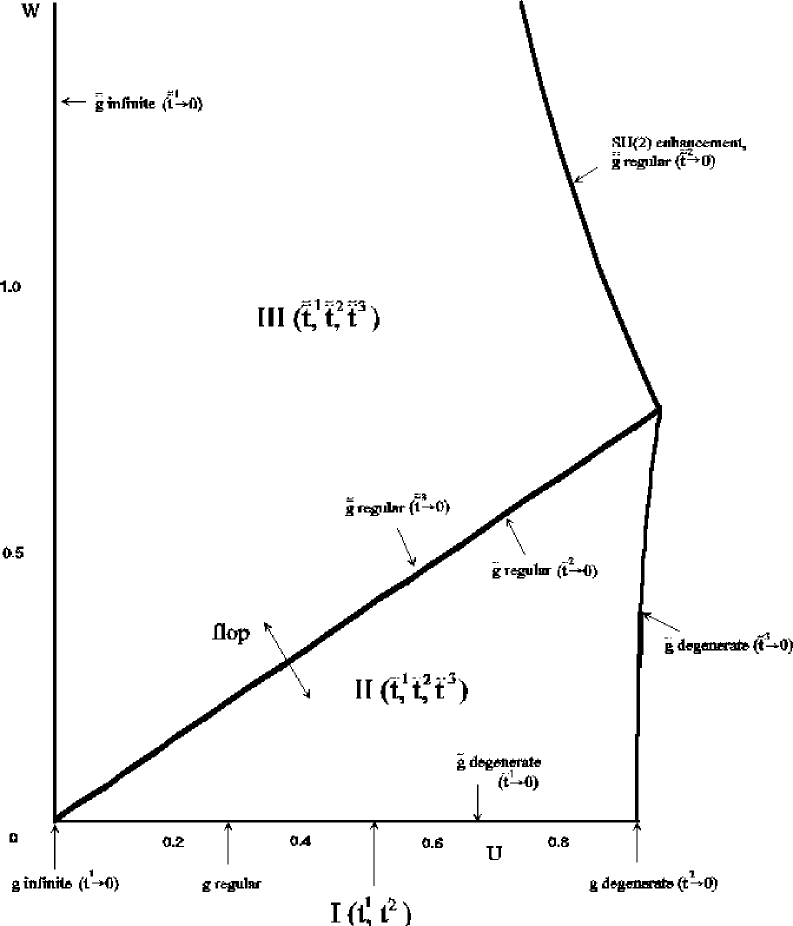
Figure 2: The extended moduli space

6.1 Model I: the Base $P_{2}$ Vacuum

This Calabi-Yau compactification corresponds to the lower boundary of Figure 2. It is a rather simple example as it admits only one independent moduli field. Yet, it incorporates rich and surprising structures.

Its prepotential is given by

$${\cal V}_{I}=9(t^{1})^{3}+9(t^{1})^{2}t^{2}+3t^{1}(t^{2})^{2}=1.$$ (6.4)

To achieve a consistent notation for all three connected models we perform a coordinate redefinition to variables $U$ and $T$, related to the basic cycles $t^{1}$ and $t^{2}$ by

$$U = 6^{\frac{1}{3}}t^{1}$$

$$T = 6^{\frac{1}{3}}(t^{2}+\frac{3}{2}t^{1}).$$ (6.5)

The constraint on the moduli fields translates to

$${\cal V}_{I}=\frac{3}{8}U^{3}+\frac{1}{2}UT^{2}=1.$$ (6.6)

For convenience we choose $U$ as an independent variable. In this case, $T$ is given by

$$T=\sqrt{\frac{2}{U}(1-\frac{3}{8}U^{3})}.$$ (6.7)

Note that it is the basic cycles $t^{1},t^{2}$ of the Calabi-Yau manifold and not the $T,\,\,U$ variables which should be restricted to be positive.

To understand the structure of the moduli space one has to compute the metric which in this case is a scalar. It is determined to be

$$g=\frac{6-9U^{3}}{8U^{2}-3U^{5}}.$$ (6.8)

Important are also the gauge couplings. We do not give the explicit form of $G_{IJ}$ here but note that its determinant is given by

$$\det G_{IJ}=\frac{1}{24\times 6^{1/3}U}(1-\frac{3}{2}U^{3}).$$ (6.9)

In the region $0\leq t^{1},t^{2}$, $g$ and $\det G$ are regular as expected. They diverge at $t^{1}\sim U=0$ and degenerate at

$$U_{0}=(\frac{2}{3})^{1/3}.$$ (6.10)

This is also the point where $t^{2}$ turns negative. Hence, $0\leq U\leq U_{0}$ defines the domain of validity. The regularity of $T$ in this region and on the boundary $t^{2}=0$ is quite crucial as it implies that $Z$ and $\partial Z$ are regular here also.

These considerations allow us to predict some properties of the potentials. First of all, for a range of charge configurations $(q_{U},q_{T})$ we do expect a critical point of the central charge in the regular domain which in turn is a minimum of the potentials $V$ and $P$.

Since $T$ diverges at $U\rightarrow 0$ all three potentials diverge to positive infinity at this boundary of the moduli space. On the other side of the domain of validity, $Z$ and $\partial Z$ are regular but $g^{-1}\rightarrow\infty$, hence $V$ generically diverges to positive infinity whereas $P$ turns negative towards infinity. This implies a second new critical point for potentials of gauged supergravities! In fact, this extrema must be a maximum of $P$ (implying a minimum of the gauge potential, as we flipped the sign for convenience).

The second prediction we can make is that $V$ always admits a minimum, as on both boundaries it diverges to positive infinity.

Let us verify our general considerations. First we solve the stabilization equations, leading to the critical points of the central charge. The charges are denoted by $(q_{U},q_{T})$ where we take $q_{U}\geq 0$ without loss of generality, since $(q_{U},q_{W})\rightarrow-(q_{U},q_{W})$ leaves the potentials invariant. In the domain of validity we find the solution

$$U_{\rm crit} = \frac{2}{\sqrt{3Z^{\rm crit}}}\sqrt{q_{U}-\sqrt{q_{U}^{2}-\frac{9}{4}q_{T}^{2}}}$$

$$T_{\rm crit} = \sqrt{\frac{3}{Z^{\rm crit}}}\sqrt{q_{U}+\sqrt{q_{U}^{2}-\frac{9}{4}q_{T}^{2}}}$$ (6.11)

with the central charge

$$Z^{\rm crit}=\left[q_{U}\frac{2}{\sqrt{3}}\sqrt{q_{U}-\sqrt{q_{U}^{2}-\frac{9}{4}q_{T}^{2}}}+q_{T}\sqrt{3q_{U}+3\sqrt{q_{U}^{2}-\frac{9}{4}q_{T}^{2}}}\right]^{2/3}.$$ (6.12)

The charge configurations allowing for a stabilization of the central charge are constrained by

$$q_{U}\geq\frac{3}{2}q_{T}\geq 0.$$ (6.13)

As anticipated, in the domain $g>0$ ($t^{1},t^{2}>0$) we find precisely one extremum of the central charge (6.13). This should coincide with the extremum of the potentials according to our considerations of the last section. We will not give the explicit form of $V$ and $P$ here as functions of $U$ but rather consider the specific charge configurations $q_{U}=4,q_{T}=2$ and $q_{U}=2,q_{T}=2$. The results are plotted in Figure 3. This can be done without much loss of generality as the general structure of the potentials is rather insensitive to a specific choice of charges, as long as we avoid the boundary values $q_{T}=\frac{2}{3}q_{U}$ and $q_{T}=0$.

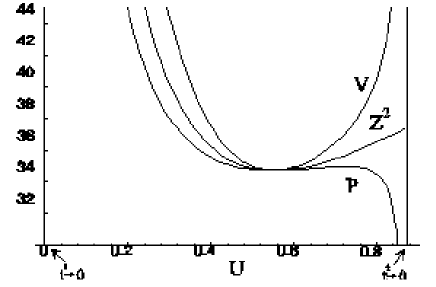
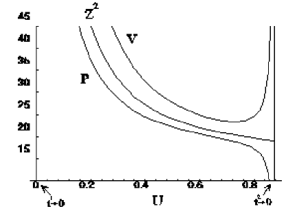
Figure 3: $Z^{2}$, $V$ and $P$ for $(q_{U},q_{W})=(4,2)$ (left) and $(q_{U},q_{T})=(2,2)$ (right)

For the first set of charges the picture is as expected. The minima of $Z^{2},P$ and $V$ coincide exactly at the position predicted by (6.11). However, $P$ indeed admits a new maximum which does not correspond to critical points of the central charge.

The situation is very different for the configuration $(q_{U},q_{T})=(2,2)$. The central charge does not get stabilized anymore, also $P$ does not admit critical points. However, $V$ still has a minimum in agreement with our discussion above. This minimum corresponds to the stabilized values of the moduli in the non-supersymmetric extreme black hole solution with the same charges. In fact one finds that for all charge configurations stabilization of the scalar potential takes place!

There are also the two boundary points:

$$q_{U}=\frac{3}{2}q_{T}\ \ \ \ {\rm and}\ \ \ \ q_{T}=0.$$ (6.14)

Here, we find stabilization at the boundaries (i.e. on the singularities) and the potentials become finite there. An example is given in Figure 4, where the charge configuration $(q_{U},q_{T})=(3,2)$ is shown to admit stabilization at the point $U=U_{0}$, i.e. at $t^{2}=0$.

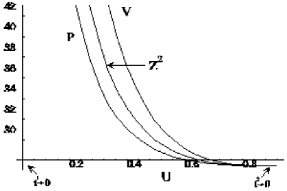
Figure 4: $Z^{2},V,P$ for $q_{U}=3,\ q_{T}=2$

This is rather peculiar as it implies that stabilization takes place right on the edge of a Calabi-Yau space. Stabilization at $t^{1}=0$ occurs for $q_{T}=0$.

To summarize the discussion of $V$ we emphasize again that in this example for all charge configurations $V$ has a minimum in the allowed region of moduli fields (or on its boundaries), as opposed to $Z$ and $P$, where extrema are found only when (6.13) is satisfied.

It is known (see for example [42]) that in this Calabi-Yau manifold 29 complex structure moduli can be shrunk to zero size, and the resulting singularity can be resolved by blowing up a four-cycle. In this manner we obtain a new Calabi-Yau manifold with one more Kähler moduli field, which will be discussed now.

6.2 Model II: the Base $F_{1}$ Vacuum

This space (model II of Figure 2) is more complex than the previous one. Nevertheless, the general structure of critical points is similar to what we have learned above.

If a complex divisor is blown up in the $P_{2}$ space, resulting in a new two-cycle $W$, it turns out that the new prepotential is given by [42]

$${\cal V}_{II}=\frac{3}{8}U^{3}+\frac{1}{2}UT^{2}-\frac{1}{6}W^{3}.$$ (6.15)

Clearly, in the limit $W\rightarrow 0$ one recovers (6.6).

To find the boundary of this Kähler cone a transformation to the basic cycles

$$\tilde{t}^{1} = W$$

$$\tilde{t}^{2} = U-W$$ (6.16)

$$\tilde{t}^{3} = T-\frac{3}{2}U$$

has to be performed in terms of which the prepotential becomes

$${\cal V}_{II}=\frac{4}{3}(\tilde{t}^{1})^{3}+\frac{3}{2}(\tilde{t}^{2})^{3}+\frac{9}{2}(\tilde{t}^{1})^{2}\tilde{t}^{2}+\frac{9}{2}\tilde{t}^{1}(\tilde{t}^{2})^{2}+\frac{3}{2}(\tilde{t}^{1})^{2}\tilde{t}^{3}+\frac{3}{2}(\tilde{t}^{2})^{2}\tilde{t}^{3}+\frac{1}{2}\tilde{t}^{1}(\tilde{t}^{3})^{2}+\frac{1}{2}\tilde{t}^{2}(\tilde{t}^{3})^{2}+3\tilde{t}^{1}\tilde{t}^{2}\tilde{t}^{3},$$ (6.17)

and the domain of this Kähler cone is then defined by $\tilde{t}^{I}\geq 0$.

For the discussion of the critical points the variables $(U,T,W)$ are more convenient. If we choose $U$ and $W$ as independent variables, the constraint ${\cal V}_{II}=1$ leads to

$$T=\sqrt{\frac{24-9U^{3}+4W^{3}}{12U}}$$ (6.18)

and the determinant of the moduli space metric is given by

$$\det\tilde{g}_{ij}=\frac{3W(6-9U^{3}+W^{3})}{2U^{2}(24-9U^{3}+4W^{3})}.$$ (6.19)

The determinant of the gauge couplings is found to be

$$\det\tilde{G}_{IJ}=\frac{W}{288U}-\frac{U^{2}W}{192}+\frac{W^{4}}{1728U}.$$ (6.20)

The boundary of the Kähler cone is reached by setting one (or more) of the fundamental cycles to zero. At these points one can have a flop transition or reaches the end of the extended Kähler cone. At $\tilde{t}^{1}=W=0$ (lower boundary in Fig. 2) we find $\det\tilde{g}_{ij}=0$ and we recover model I as mentioned before. The moduli space metric also degenerates at the boundary $\tilde{t}^{3}=T-\frac{3}{2}U=0$ (right boundary in Fig. 2). We note that some gauge fields become strongly coupled at these boundaries.

$\tilde{t}^{2}=U-W\rightarrow 0$ (upper left boundary) turns out to be a flop transition. Here, the metrics are completely regular and very special geometry is still valid if we pass this boundary. However, physically we enter the new Calabi-Yau space of model III with different intersection numbers.

We begin the discussion of critical points with a few general observations. If we choose a charge configuration which allows for a stabilization of the central charge then the arguments given for model I do apply again and we can deduce some of the properties of the potentials. Consider first $P$. At each of the two intersecting $\det\tilde{g}=0$ lines (i.e. $\tilde{t}^{1}=0$ and $\tilde{t}^{3}=0$) $P$ is expected to diverge to negative infinity. As the supersymmetric stabilization point must be a minimum, there ought to be three additional critical points: two saddle points and one maximum. Hence, we learn once more that the structure of critical points of gauged supergravities is rather rich. We also expect that $V$ has new critical points for charge configurations which do not stabilize $Z$ in the valid domain.

As for model I we verify our intuition by solving the stabilization equations and study the potentials with specific charge configurations. We find that the extremum of the central charge in the valid region is located at

$$U_{\rm crit} = \frac{2}{\sqrt{3Z^{\rm crit}}}\sqrt{q_{U}-\sqrt{q_{U}^{2}-\frac{9}{4}q_{T}^{2}}}$$

$$T_{\rm crit} = \sqrt{\frac{3}{Z^{\rm crit}}\sqrt{q_{U}+\sqrt{q_{U}^{2}-\frac{9}{4}q_{T}^{2}}}}$$ (6.21)

$$W_{\rm crit} = \sqrt{-\frac{6}{Z^{\rm crit}}q_{W}}$$

with the critical value of the central charge

$$Z^{\rm crit}=\left(q_{U}\sqrt{\frac{4}{3}(q_{U}-\sqrt{q_{U}^{2}-\frac{9}{4}q_{T}^{2}})}+q_{T}\sqrt{3(q_{U}+\sqrt{q_{U}^{2}-\frac{9}{4}q_{T}^{2}})}+q_{W}\sqrt{-6q_{W}}\right)^{\frac{2}{3}}.$$ (6.22)

Here, $q_{U}>0$ was chosen without loss of generality due to the ${\bf Z}_{2}$ ($q^{I}\rightarrow-q^{I}$) symmetry of the potentials. Supersymmetric stabilization occurs only for the region

$$q_{U} \geq \frac{3}{2}q_{T}\geq 0$$

$$0 \geq q_{W}\geq-\frac{2}{9}\left(q_{U}-\sqrt{q_{U}^{2}-\frac{9}{4}q_{T}^{2}}\right).$$ (6.23)

At the critical values (saturation of above inequalities) $Z$ gets stabilized on the boundaries of the moduli space. To be explicit, we find for $q_{U}=\frac{3}{2}q_{T}$ stabilization at $\tilde{t}^{3}=0$ and for $q_{W}=0$ at $\tilde{t}^{1}=0$. The latter observation is very much consistent with the expectation that absence of $q_{W}$ drives the internal space in the vicinity of the black hole to the $CY$ space with $P_{2}$ as a base.

If

$$q_{W}<-\frac{2}{9}\left(q_{U}-\sqrt{q_{U}^{2}-\frac{9}{4}q_{T}^{2}}\right)$$ (6.24)

no stabilization occurs in the present Kähler cone. In fact, what we observe is that the critical point moves over the boundary $\tilde{t}^{2}=U-W=0$ into the adjacent Calabi-Yau space.

Let us now turn to the study of $P$ via a specific example. As a typical case with supersymmetric stabilization we consider the charge configuration

$$q_{U}=5,\quad q_{T}=2,\quad q_{W}=-\frac{1}{6},$$ (6.25)

as general properties of the potential are independent of a specific choice. Figure 5 shows beautifully the structure of $P$. This potential admits indeed four critical points as anticipated. The minimum agrees with the ones of $V$ and $Z^{2}$, the two saddle points and the maximum are new.

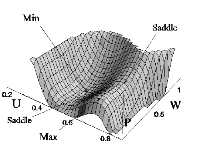
Figure 5: Potential $P$ with 4 critical points

If $q_{W}$ approaches $0$, the pairs of critical points merge on the $W=0$ line rendering the results of model I. If $q_{W}$ becomes positive, the critical points of $P$ and $Z$ disappear, however, $V$ still stabilizes, showing the same characteristics as in the last example. As long as $q_{W}$ is below a certain value, the black hole potential stabilizes in the allowed domain of this Calabi-Yau. There is some critical value for which also the non-supersymmetric stabilization of $V$ takes place in the adjoining Kähler cone in very much the same way as we already observed for $Z$. Note that $\tilde{t}^{2}=U-W$ is the only boundary where the moduli space metric is non-degenerate, hence stabilization points can smoothly “move” across this transition line.

Let us also comment on the other two boundaries. In particular, we will consider the tension of solitonic BPS strings. The tension of these solitonic objects is given by

$$Z_{m}=\tilde{t}_{I}\tilde{m}^{I}$$ (6.26)

where the $\tilde{m}^{I}$ are the winding numbers of eleven-dimensional five-branes wrapping around the four-cycles $\tilde{t}_{I}$ defined in (3.3). At the boundary $\tilde{t}^{1}\rightarrow 0$ (transition to model I) we find indeed tensionless strings consistent with the arguments given in [22]. This can be easily seen as the four-cycle moduli are given by

$$\tilde{t}_{1} = \frac{4}{3}(\tilde{t}^{1})^{2}+3\tilde{t}^{1}\tilde{t}^{2}+\frac{3}{2}(\tilde{t}^{2})^{2}+\tilde{t}^{1}\tilde{t}^{3}+\frac{1}{6}(\tilde{t}^{3})^{2}+\tilde{t}^{2}\tilde{t}^{3}$$

$$\tilde{t}_{2} = \frac{3}{2}(\tilde{t}^{1})^{2}+3\tilde{t}^{1}\tilde{t}^{2}+\frac{3}{2}(\tilde{t}^{2})^{2}+\tilde{t}^{1}\tilde{t}^{3}+\frac{1}{6}(\tilde{t}^{3})^{2}+\tilde{t}^{2}\tilde{t}^{3}$$ (6.27)

$$\tilde{t}_{3} = \frac{1}{2}(\tilde{t}^{1})^{2}+\tilde{t}^{1}\tilde{t}^{2}+\frac{1}{2}(\tilde{t}^{2})^{2}+\frac{1}{3}\tilde{t}^{1}\tilde{t}^{3}+\frac{1}{3}\tilde{t}^{2}\tilde{t}^{3}.$$

If we consider the cycle $\tilde{t}_{1}-\tilde{t}_{2}$ we find

$$\tilde{t}_{1}-\tilde{t}_{2}=-\frac{1}{6}(\tilde{t}^{1})^{2}$$ (6.28)

implying that the BPS string states with charges $\tilde{m}=\pm(1,-1,0)$ indeed become tensionless with $Z\sim(\tilde{t}^{1})^{2}$! We argue that model I is reached via this mechanism.

The boundary $\tilde{t}^{3}\rightarrow 0$ shows the same characteristics, the moduli space metric degenerates and the string states with charges

$$\tilde{m}=\pm(0,1,-3)$$ (6.29)

become tensionless also with tension $\sim(\tilde{t}^{3})^{2}$.

As expected, at the flop transition $\tilde{t}^{2}=0$ it is straightforward to verify that none of the string states becomes tensionless along the entire transition line, i.e. there is no linear combination of $\tilde{t}_{I}$ which vanishes here.

We will now study the flopped Calabi-Yau space in detail.

6.3 Model III: The Flopped $F_{1}$ Base

In model II $\tilde{t}^{2}=U-W\rightarrow 0$ marks a topology change of the mild form. The Hodge numbers are unaffected, but the intersection numbers $C_{IJK}$ change [25, 22]. These topological data changes lead to the new prepotential augmented by the term $-\frac{1}{6}(U-W)^{3}$

$${\cal V}_{III}=\frac{5}{24}U^{3}+\frac{1}{2}U^{2}W-\frac{1}{2}UW^{2}+\frac{1}{2}T^{2}U=1.$$ (6.30)

As discussed in section 5.1 the charges $q_{U},q_{W},q_{T}$ are in fact unchanged by this flop transition.

$U,W$ and $T$ are again not the proper Calabi-Yau variables, the correct parametrization to determine the boundary of this space is

$$\hskip 1.99168pt\tilde{\tilde{t}}\hskip 1.42262pt^{1} = U$$

$$\hskip 1.99168pt\tilde{\tilde{t}}\hskip 1.42262pt^{2} = T-\frac{1}{2}U-W$$ (6.31)

$$\hskip 1.99168pt\tilde{\tilde{t}}\hskip 1.42262pt^{3} = W-U$$

and $\hskip 1.99168pt\tilde{\tilde{t}}\hskip 1.42262pt^{I}>0$ defines this Kähler cone. In these variables the prepotential becomes

$${\cal V}_{III}=\frac{4}{3}(\hskip 1.99168pt\tilde{\tilde{t}}\hskip 1.42262pt^{1})^{3}+\frac{3}{2}(\hskip 1.99168pt\tilde{\tilde{t}}\hskip 1.42262pt^{1})^{2}\hskip 1.99168pt\tilde{\tilde{t}}\hskip 1.42262pt^{2}+\frac{1}{2}\hskip 1.99168pt\tilde{\tilde{t}}\hskip 1.42262pt^{1}(\hskip 1.99168pt\tilde{\tilde{t}}\hskip 1.42262pt^{2})^{2}+(\hskip 1.99168pt\tilde{\tilde{t}}\hskip 1.42262pt^{1})^{2}\hskip 1.99168pt\tilde{\tilde{t}}\hskip 1.42262pt^{3}+\hskip 1.99168pt\tilde{\tilde{t}}\hskip 1.42262pt^{1}\hskip 1.99168pt\tilde{\tilde{t}}\hskip 1.42262pt^{2}\hskip 1.99168pt\tilde{\tilde{t}}\hskip 1.42262pt^{3}=1.$$ (6.32)

The potentials are again analyzed in $(U,T,W)$ variables. Due to the constraint, $T$ is now given by

$$T=\frac{6-8U^{3}-9U^{2}W-3UW^{2}}{6U(U+W)}.$$ (6.33)

We find for the moduli space metric and gauge couplings

$$\det\hskip 0.85358pt\tilde{\tilde{g}}\hskip 1.42262pt_{ij}=\frac{3-4U^{3}}{4U^{2}(U+W)^{2}}$$ (6.34)

and

$$\det\hskip 0.85358pt\tilde{\tilde{G}}\hskip 1.42262pt_{IJ}=\frac{3-4U^{3}}{864}.$$ (6.35)

Hence, $\hskip 0.85358pt\tilde{\tilde{g}}\hskip 1.42262pt$ diverges at $\hskip 1.99168pt\tilde{\tilde{t}}\hskip 1.42262pt^{1}\rightarrow 0$, (left boundary of Fig. 2), but is regular at $\hskip 1.99168pt\tilde{\tilde{t}}\hskip 1.42262pt^{2}\rightarrow 0$ (right boundary) and $\hskip 1.99168pt\tilde{\tilde{t}}\hskip 1.42262pt^{3}\rightarrow 0$ (lower boundary). Regularity at the latter transition is no surprise, as we have just pass back into the Calabi-Yau space of above via the flop. However, $\hskip 1.99168pt\tilde{\tilde{t}}\hskip 1.42262pt^{2}\rightarrow 0$ marks the end of the moduli space in finite distance. We will later interpret this line as the transition where a divisor shrinks to a complex curve. Noteworthy is that, as all metrics are regular here, there is no protection that ensures stabilization before the boundary, not even for $V$.

As the behavior of the potentials is generically not very different from model II we will not give many details. Nevertheless it is useful to consider the supersymmetric stabilization points

$$U_{\rm crit} = \frac{1}{2Z_{\rm crit}^{\frac{1}{2}}}\sqrt{6q_{U}+3q_{W}-3\sqrt{4q_{U}^{2}+4q_{U}q_{W}+9q_{W}^{2}-8q_{T}^{2}}}$$

$$T_{\rm crit} = \frac{3q_{T}}{U}=\frac{6q_{T}}{Z_{\rm crit}^{\frac{1}{2}}\sqrt{6q_{U}+3q_{W}-3\sqrt{4q_{U}^{2}+4q_{U}q_{W}+9q_{W}^{2}-8q_{T}^{2}}}}$$ (6.36)

$$W_{\rm crit} = \frac{U^{2}-6q_{W}}{2U}=\frac{6q_{U}-21q_{W}-3\sqrt{4q_{U}^{2}+4q_{U}q_{W}+9q_{W}^{2}-8q_{T}^{2}}}{4Z_{\rm crit}^{\frac{1}{2}}\sqrt{6q_{U}+3q_{W}-3\sqrt{4q_{U}^{2}+4q_{U}q_{W}+9q_{W}^{2}-8q_{T}^{2}}}}.$$

With some algebra we find that supersymmetric stabilization takes place if

$$q_{U}\geq\frac{3}{2}q_{T}\geq 0$$ (6.37)

and

$$q_{W}\leq-\frac{2}{9}\left(q_{U}-\sqrt{q_{U}^{2}-\frac{9}{4}q_{T}^{2}}\right).$$ (6.38)

If (6.37) is saturated the critical point lies directly on the $\hskip 1.99168pt\tilde{\tilde{t}}\hskip 1.42262pt^{2}=T-\frac{1}{2}U-W=0$ (right) boundary, whereas saturation of (6.38) implies stabilization on the flop transition line $\hskip 1.99168pt\tilde{\tilde{t}}\hskip 1.42262pt^{3}=W-U=0$. In fact, the stabilization points of model II and model III agree with each other for such a configuration as predicted. In both cases, the moduli metric and the gauge couplings are finite. At the flop transition we expect $Z,\partial Z$ and $V$ to be continuous. However, $V$ should have a kink, according to our discussion in section 5.1. Figure 6 and 7 graphically illustrate this behavior. The minima of $V$ and $Z^{2}$ are marked by an ellipse.

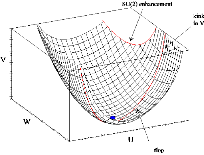
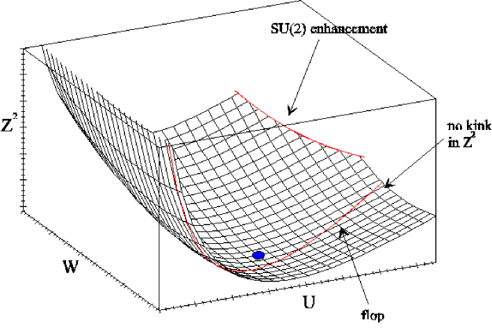
Figure 6: Continuity and kink of $V$

Figure 7: Continuity and smoothness of $Z^{2}$

Figure 8 shows how the stabilization point smoothly moves over the flop boundary if we vary $q_{W}$.

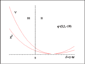
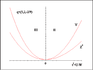
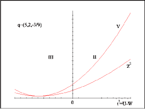
Figure 8: Stabilization for configurations $(q_{U},q_{T},q_{W})=(5,2,-1/9),(5,2,-2/9),(5,2,-3/9)$

The right hand side boundary $\hskip 1.99168pt\tilde{\tilde{t}}\hskip 1.42262pt^{2}=T-\frac{1}{2}U-W=0$ is different in the sense that there is no flop transition to another Calabi-Yau space possible, although the metric is also regular. Hence, the conclusion is that this line corresponds to an end of the moduli space in finite distance. Let us see again whether strings become tensionless at this point. Indeed, one finds that the magnetic central charge for string states with charges

$$\hskip 1.99168pt\tilde{\tilde{m}}\hskip 1.42262pt=\pm(1,-2,1)$$ (6.39)

vanishes. However, in this case $Z_{m}$ behaves as

$$Z_{m}\sim\hskip 1.99168pt\tilde{\tilde{t}}\hskip 1.42262pt^{2}$$ (6.40)

which implies that the tension of the string is decreasing much slower than we found for the two non-flop boundaries of model II. This behavior again agrees with the one expected in [22] for the case where a divisor shrinks to a curve and symmetry enhancement to $SU(2)$ takes place. This symmetry enhancement is indeed expected in our model, as one can perform a redefinition of variables to write the prepotential as ${\cal V}_{III}=S^{\prime}T^{\prime}U^{\prime}-\frac{1}{3}U^{\prime 3}$. In these variables $\hskip 1.99168pt\tilde{\tilde{t}}\hskip 1.42262pt^{2}\rightarrow 0$ corresponds to $T^{\prime}=U^{\prime}$ which is known to be a symmetry enhancement point.

At the other boundary $\hskip 1.99168pt\tilde{\tilde{t}}\hskip 1.42262pt^{1}\rightarrow 0$ we again find the phenomenon of strings becoming tensionless faster than any particle becomes massless. We observe that at the end of the moduli space of our example special geometry remains valid if a divisor shrinks to a curve. If the divisor shrinks to a point, special geometry breaks down and the moduli space metric and gauge couplings degenerate or diverge.

7 Conclusions

In this paper we have studied phase transition of $d=5$ M-theory compactifications on Calabi-Yau three-folds. We have probed the nature of the phase transitions utilizing several physical potentials including the electric BPS mass $Z$, the magnetic string tension $Z_{m}$, the black hole potential $V$ and the gauged central charge potential $P$. They are direct supersymmetric and supergravity analogs of the Landau-Ginzburg potentials used in thermodynamic systems that undergo phase transitions.

A lot of attention recently was directed to the properties of the entropy of the extreme black holes. The entropy is given by the area of the horizon and is related to the size of the infinite throat of $adS_{2}$. It has a topological origin, being independent on the values of moduli far away from the horizon [14]. The value of the entropy is given by the central charge extremized in the moduli space [15]. We found that in five dimensions the corresponding stabilization equations take an extremely simple form.

For the extended objects $p>0$ other than black holes, which have a vanishing area of the horizon, the analogous critical behavior was not studied before. Here we have found that the tension of the magnetic string which is not equal to the area of the horizon, but describes a size of an infinite throat of $adS_{3}$, is given by a critical value of the magnetic central charge. We found that the tension of the magnetic string in 5d can take a minimal value $T^{3}=C_{IJK}m^{I}m^{J}m^{K}$ for a given choice of winding numbers $m^{I}$ of an 11d fivebrane wrapped on four-cycles inside the CY space. We expect that new results on critical behavior of various extended objects will emerge based on these results.

We also have shown explicitly that $V$ and $P$ admit new extrema which are not related to supersymmetric stabilization.

One of the main goal in this work was to obtain a better understanding of the structure of the above supersymmetry potentials in the entire extended Kähler cone. In $d=5$, because of absence of non-geometric phases, the extended Kähler cone is generically a geodesically incomplete, bounded domain. Since $Z$ and $\partial Z$ turned out to be continuous across flop transitions, and any critical point of $Z$ must be a minimum, we were able to draw the important conclusion that supersymmetric stabilization can take place in at most one point in the entire extended Kähler cone. The same conclusion was drawn for the string tension $Z_{m}$. The analytic properties of $V$ were shown to be slightly different. At the flop $V$ is continuous but not differentiable. It remains to be shown that also the critical point of $V$ (for fixed charges) is unique. This result would prove that the black hole entropy is unaffected even though a topology change takes place as one moves away from the black hole horizon to spatial infinity.

Finally we have studied in detail several explicit examples of Calabi-Yau compactifications with small dimensions of the Kähler moduli space. We have verified our general results of previous sections on these examples and found that at the boundaries of the extended Kähler cone, BPS magnetically charged strings become tensionless. In some cases, these tensionless strings can be related to extremal phase transitions to Calabi-Yau spaces with different Hodge numbers.

8 Acknowledgments

We are grateful for useful discussions with P. Candelas, S. Ferrara, E. Gimon, C. Johnson, X. de la Ossa, Y. Oz and E. Witten. The work of R.K., J.R., M.S. and W.K.W. is supported by the NSF grant THY-9219345. The work of M.S. is also supported by the Department of Energy under contract DOE-DE-FG05-91ER40627. The work of S.-J. R. is supported in part by DOE DE-FG-02-90ER40542, NSF Grant PHY-9513835, NSF-KOSEF Bilateral Grant, KOSEF Purpose-Oriented Research Grant and SRC Program, Ministry of Education BSRI Program 97-2410 and the Monell Foundation and the Seoam Foundation Fellowships.

References

- [1] E. Witten, String theory dynamics in various dimensions, Nucl. Phys. B443 (1995) 85.
- [2] E. Cremmer, B. Julia and J. Scherk, Supergravity theory in eleven-dimensions, Phys. Lett. 76B (1978) 409.
- [3] E. Witten, Strong coupling expansion of Calabi-Yau compactification, Nucl. Phys. B471 (1996) 135.
- [4] H. P. Nilles and S. Stieberger, String-unification, universal one-loop corrections and strongly coupled heterotic string theory, hep-th/9702110 (1997).
- [5] A. C. Cadavid, A. Ceresole, R. D’Auria and S. Ferrara, Eleven-dimensional supergravity compactified on Calabi-Yau threefolds, Phys. Lett. B357 (1995) 76.
- [6] S. Ferrara, R. R. Khuri and R. Minasian, M-theory on a Calabi-Yau manifold, Phys. Lett. B375 (1996) 81.
- [7] A. Strominger, Massless black holes and conifolds in string theory, Nucl. Phys. B451 (1995) 96.
- [8] E. Witten, Small instantons in string theory, Nucl. Phys. B460 (1996) 541.
- [9] E. Witten, Some comments on string dynamics, hep-th/9507121 (1995).
- [10] O. J. Ganor and A. Hanany, Small instantons and tensionless non-critical strings, Nucl. Phys. B474 (1996) 122.
- [11] N. Seiberg and E. Witten, Comments on string dynamics in six dimensions, Nucl. Phys. B471 (1996) 121.
- [12] M. J. Duff, H. Lu and C. N. Pope, Heterotic phase transitions and singularities of the gauge dyonic string, Phys. Lett. B378 (1996) 101.
- [13] N. Kim, S.-J. Rey, S. Theisen and S. Yankielowitz, Non-perturbative heterotic string vacua and tensionless gravitational strings, (to appear).
- [14] S. Ferrara, R. Kallosh and A. Strominger, N=2 extremal black holes, Phys. Rev. D52 (1995) 5412.
- [15] S. Ferrara and R. Kallosh, Supersymmetry and attractors, Phys. Rev. D54 (1996) 1514.
- [16] S. Ferrara and R. Kallosh, Universality of supersymmetric attractors, Phys. Rev. D54 (1996) 1525.
- [17] R. Kallosh, M. Shmakova and W. K. Wong, Freezing of moduli by N= 2 dyons, Phys. Rev. D54 (1996) 6284.
- [18] K. Behrndt, R. Kallosh, J. Rahmfeld, M. Shmakova and W. K. Wong, STU black holes and string triality, Phys. Rev. D54 (1996) 6293.
- [19] K. Behrndt, G. L. Cardoso, B. de Wit, R. Kallosh, D. Lüst and T. Mohaupt, Classical and quantum N=2 supersymmetric black holes, hep-th/9610105 (1996).
- [20] S.-J. Rey, Classical and quantum aspects of bps black holes in N = 2, d = 4 heterotic string compactifications, hep-th/9610157 (1996).
- [21] K. Behrndt and W. A. Sabra, Static N=2 black holes for quadratic prepotentials, hep-th/9702010 (1997).
- [22] E. Witten, Phase Transitions in M-Theory and F-Theory, Nucl. Phys. B471 (1996) 195.
- [23] S. Ferrara, C. Kounnas, D. Lüst, F. Zwirner, Duality invariant partition functions and automorphic superpotentials for (2,2) string compactifications, Nucl. Phys. B365 (1991) 431.
- [24] B. de Wit and A. V. Proeyen, Broken Sigma-Model Isometries in Very Special Geometry, Phys. Lett. B293 (1992) 94.
- [25] I. Antoniadis, S. Ferrara and T. R. Taylor, N=2 heterotic superstring and its dual theory in five dimensions, Nucl. Phys. B460 (1996) 489.
- [26] B. de Wit, P. G. Lauwers and A. Van Proeyen, Lagrangians of N=2 supergravity - matter systems, Nucl. Phys. B255 (1985) 569.
- [27] K. Becker, M. Becker and A. Strominger, Fivebranes, membranes and nonperturbative string theory, Nucl. Phys. B456 (1995) 130.
- [28] M. Gunaydin, G. Sierra and P. K. Townsend, The geometry of N=2 Maxwell-Einstein supergravity and Jordan algebras, Nucl. Phys. B242 (1984) 244.
- [29] A. Chamseddine, S. Ferrara, G. W. Gibbons and R. Kallosh, Enhancement of supersymmetry near 5d black hole horizon, Phys. Rev. D55 (1997) 3647.
- [30] M. Shmakova, Calabi-Yau black holes, hep-th/9612076 (1996).
- [31] K. Behrndt and T. Mohaupt, Entropy of N = 2 black holes and their m-brane description, hep-th/9611140 (1996).
- [32] J. Maldacena, N = 2 extremal black holes and intersecting branes, hep-th/9611163 (1996).
- [33] K. Behrndt, Decompactification near the horizon and non-vanishing entropy, hep-th/9611237 (1996).
- [34] S. Ferrara, G. W. Gibbons and R. Kallosh, Black holes and critical points in moduli space, (1997).
- [35] P. Breitenlohner, D. Maison and G. Gibbons, Four-dimensional black holes from Kaluza-Klein theories, Commun. Math. Phys. 120 (1988) 295.
- [36] G. Gibbons, R. Kallosh and B. Kol, Moduli, scalar charges, and the first law of black hole thermodynamics, Phys. Rev. Lett. 77 (1996) 4992.
- [37] S. B. Giddings, J. Polchinski and A. Strominger, Four-dimensional black holes in string theory, Phys. Rev. D48 (1993) 5784.
- [38] R. R. Khuri and T. Ortin, A nonsupersymmetric dyonic extreme Reissner-Nordstrom black hole, Phys. Lett. B373 (1996) 56.
- [39] M. J. Duff and J. Rahmfeld, Bound states of black holes and other p-branes, Nucl. Phys. B481 (1996) 332.
- [40] M. J. Duff, J. T. Liu and J. Rahmfeld, Dipole moments of black holes and string states, hep-th/9612015 (1996).
- [41] T. Ortin, Extremality versus supersymmetry in stringy black holes, hep-th/9612142 (1996).
- [42] J. Louis, J. Sonnenschein, S. Theisen and S. Yankielowicz, Non-perturbative properties of heterotic string vacua compactified on K3 x T2, Nucl. Phys. B480 (1996) 185.
- [43] D. R. Morrison and C. Vafa, Compactifications of F-theory on Calabi–Yau threefolds – II, Nucl. Phys. B476 (1996) 437.
- [44] P. Candelas, A. Font, S. Katz and D. R. Morrison, Mirror symmetry for two parameter models. 2, Nucl. Phys. B429 (1994) 626.