Abstract

April 16 1997

1 Introduction

Dualities and nonperturbative phenomena in string theory have been a subject of extensive study for the last two years. Beginning with the work of refs. [4, 5, 6] it has been realized that compactifications of string theories on singular spaces lead to extra massless degrees of freedom and hence to a variety of possibilities for new connections between apparently different string theories. In particular, in [5] it was conjectured for the first time that if a type IIA string is compactified on a $K3$ surface with an orbifold singularity then the resulting theory can exhibit a simply-laced nonabelian gauge group of the type which matches exactly the $ADE$ singularity type of the $K3$ surface in question. Consequently, similar statements were made about type II strings compactified on Calabi–Yau threefolds. Namely, in [6] it was shown that a conifold type singularity leads to the appearance of massless black hole hypermultiplets in the low energy theory, and it was anticipated in [7, 8, 9] and shown in [10] that a curve of singularities brings about the occurrence of an enhanced gauge symmetry. The latter fact, among other things, makes possible the duality between heterotic strings on $K3\times T^{2}$ and type IIA on a Calabi–Yau threefold leading to $N=2$ supersymmetry in four dimensions, the study of which was pioneered in [11] and continued in numerous articles.

On the type II side of this duality, the enhanced gauge symmetry appears nonperturbatively and is due to the fact that the compactification manifold is singular. It has to be a $K3$ fibration [12, 13], and if we are interested in constructing duals to perturbative heterotic vacua, the singularity in question is an orbifold singularity of a generic fiber [9]. The singularity type (according to $ADE$ classification) is nothing else than the type of the gauge group appearing in the low energy theory. Going to the Coulomb branch of the latter means resolving the singularities by means of consecutive blow-ups. The intersection pattern of rational curves introduced in the process reproduces the Dynkin diagram of the gauge group.

Switching off Wilson lines on $T^{2}$ and making the torus big, this duality can be lifted to six dimensions. The Calabi–Yau manifold then must be an elliptic fibration and the type IIA string becomes F-theory on that Calabi–Yau [14]. F-theory provides a powerful tool for constructing duals to heterotic vacua [15, 16]. The gauge groups appearing in the compactified theory are due to the degeneration of the elliptic fiber over a codimension one locus in the base. A detailed dictionary between such geometric data and physics was given in [17].

The authors of [18] studied the Heterotic/Type II duality in four dimensions by means of toric geometry. They constructed reflexive polyhedra describing the (resolved version of) the singular Calabi–Yau threefolds for the type II side. They observed a regular structure present in the polyhedra. In particular, the generic $K3$ fiber could be identified as a subpolyhedron and the Dynkin diagrams of the gauge groups present in four dimensions (including non-simply laced ones) were visible directly in the subpolyhedron. Later in [19, 20, 21] it was further demonstrated that the methods of toric geometry allow one to easily read off the essential information from the corresponding polyhedra and construct Calabi–Yau manifolds relevant to different aspects of string dualities. The relation between enhanced gauge symmetry and toric diagrams was also noted in [22, 23].

The purpose of the present article is to explain the appearance of Dynkin diagrams in the examples of [18] as well as give a dictionary between the structure of the polyhedra and geometry (and hence physics) which is used in [21] to find the spectra of F-theory compactified on Calabi–Yau threefolds with large numbers of Kähler class parameters.

The paper is organized as follows. In section 2, we give some background information about divisors and intersection theory on toric varieties and the construction of Calabi–Yau hypersurfaces. In section 3, we show how to calculate the Picard lattice of a toric $K3$ manifold, or in other words, how to determine the orbifold singularity type which results upon blowing down the rational curves in the Picard lattice. In section 4, we specialize to the case of an elliptic $K3$ and show that the Dynkin diagrams of [18] appear in a natural way. Section 5 is devoted to the study of a Calabi–Yau threefold case. In particular we demonstrate the appearance of Dynkin diagrams of non-simply laced groups. Finally, section 6 summarizes our results and contains a brief discussion of more complicated cases not covered in this work.

2 Toric Preliminaries

2.1 Divisors in Toric Varieties and their Intersections

In this section we will give a brief review of the facts concerning intersection theory on toric varieties which are relevant for the following discussion. We assume the reader’s familiarity with basic notions of toric geometry, such as the definitions of cones and fans (see, e.g., [24] or [25]). We use standard notation, denoting the dual lattices by $M$ and $N$, their real extensions by $M_{\mathbb{R}}$ and $N_{\mathbb{R}}$, and the fan in $N_{\mathbb{R}}$ by $\Sigma$.

A fan $\Sigma$ in $N_{\mathbb{R}}$ defines a toric variety denoted by $X(\Sigma)$. Let $\tau$ be any $k$-dimensional cone in $\Sigma$ and $N_{\tau}$ be the sublattice of $N$ generated by $\tau\cap N$ and

$$N(\tau)=N/N_{\tau}.$$ (1)

The images in $N(\tau)$ of the cones in $\Sigma$ that contain $\tau$ as a face form a fan in $N(\tau)$ denoted by Star$(\tau)$. Then

$$V(\tau)=X({\rm Star}(\tau))$$ (2)

is an $(n-k)$-dimensional closed subvariety of $X(\Sigma)$. $V(\tau)$ is called the orbit closure. (A toric variety $X(\Sigma)$ is a disjoint union of orbits $O_{\tau}$ of the torus action, one such orbit corresponding to each cone $\tau$ in $\Sigma$.)

The Chow group $A_{n-k}$ on an arbitrary toric variety $X(\Sigma)$ is generated by the classes of the orbit closures $V(\tau)$ of the cones $\tau$ of dimension $k$. In particular, each edge (one-dimensional cone) $\tau_{i}$, generated by a unique lattice vector $v_{i}$, gives rise to a T-Weil divisor

$$D_{i}=V(\tau_{i}).$$ (3)

Suppose $D$ is a Cartier divisor on a variety $X$ and $V$ is an irreducible subvariety of $X$ which $D$ meets properly. In this case we can define an intersection cycle $D\cdot V$ by restricting $D$ to $V$, determining a Cartier divisor $D|_{V}$ on $V$, and taking the Weil divisor of this Cartier divisor: $D\cdot V=[D|_{V}]$. Now, take $X$ to be a toric variety, $D=\sum a_{i}D_{i}$ a T-Cartier divisor, and $V=V(\tau)$. In this case we obtain

$$D\cdot V(\tau)=\sum b_{\gamma}V(\gamma),$$ (4)

where the sum is over all cones $\gamma$ containing $\tau$ with dim$(\gamma)={\rm dim}(\tau)+1$, and $b_{\gamma}$ are integers computed in the following way. Suppose $\gamma$ is spanned by $\tau$ and a set of minimal edge vectors $v_{i}$. Let $e$ be the generator of the one-dimensional lattice $N_{\gamma}/N_{\tau}$ such that the image of each $v_{i}$ in $N_{\gamma}/N_{\tau}$ is $s_{i}\cdot e$ with $s_{i}$ integers. Then $b_{\gamma}$ is given by the formula

$$b_{\gamma}={a_{i}\over s_{i}},$$ (5)

all $i$’s giving the same result. If $X$ is nonsingular, then there is only one $i$ and $s_{i}=1$, so $b_{\gamma}$ is the coefficient of $D_{i}$ in $D$. In this case, $D_{k}$ is a Cartier divisor, and

$$D_{k}\cdot V(\tau)=\left\{\begin{array}[]{ll}V(\gamma)&\mbox{if $\tau$ and $v_{k}$ span a cone $\gamma$}\\ 0&\mbox{if $\tau$ and $v_{k}$ don't span a cone in $\Sigma$}\end{array}\right.$$ (6)

We can now use (6) one more time to obtain a formula for the triple intersection $D_{j}\cdot D_{k}\cdot V(\tau)$ and so on. In particular, when $\tau$ itself is a one-dimensional cone we obtain the following formula for the intersection of Cartier (Weil) divisors on a nonsingular toric variety

$$D_{k_{1}}\cdot D_{k_{2}}\cdot\ldots\cdot D_{k_{m}}=\left\{\begin{array}[]{ll}V(\gamma)&\mbox{if $v_{k_{i}}$, $i=1,\ldots m$, span a cone $\gamma$}\\ 0&\mbox{if $v_{k_{i}}$, $i=1,\ldots m$, don't span a cone in $\Sigma$}\end{array}\right.$$ (7)

If we are interested in the intersection of $n$ divisors, i.e. $m=n$ in (7), we arrive at the intersection number. Namely, provided the $v_{k_{i}}$ in (7) span an $n$-dimensional cone $\gamma$, $D_{k_{1}}\cdot D_{k_{2}}\cdot\ldots\cdot D_{k_{m}}=X({\rm Star}(\gamma))$, where ${\rm Star}(\gamma)$ is simply a toric variety of dimension zero, that is a point. Thus, we finally obtain the formula for intersection number which will be of most use for us in what follows.

$$D_{k_{1}}\cdot D_{k_{2}}\cdot\ldots\cdot D_{k_{n}}=\left\{\begin{array}[]{ll}1&\mbox{if $v_{k_{i}}$, $i=1,\ldots n$, span an $n$-dimensional cone in $\Sigma$}\\ 0&\mbox{if $v_{k_{i}}$, $i=1,\ldots n$, don't span a cone in $\Sigma$}\end{array}\right.$$ (8)

Not all of $D_{k}$’s are linearly independent though. There are certain relations between them which can be described as follows. Let $m\in M$. Then it can be shown that

$$[{\rm div}(f)]=\sum_{i}\langle m,v_{i}\rangle D_{i},$$ (9)

where $f$ is a certain nonzero rational function and the sum extends over all one-dimensional cones in $\Sigma$. Thus div$(f)$ is a principal divisor, i.e. the sum in the r.h.s. of (10) is linearly equivalent to zero:

$$\sum_{i}\langle m,v_{i}\rangle D_{i}~{}\sim~{}0~{}~{}~{}~{}\forall~{}m\in M.$$ (10)

It is obvious that we can write $n$ independent relations of the form (10), and hence, in general rank(Pic($X))\leq d_{1}-n$, where $d_{1}$ is the number of one-dimensional cones in $\Sigma$. If $X$ is nonsingular (in fact, it is sufficient to require that each cone in $\Sigma$ be simplicial), the above inequality becomes an equality:

$${\rm rank}({\rm Pic}(X))=d_{1}-n.$$ (11)

There is a convenient way of describing toric varieties which has been introduced in [26] and will be used in what follows. Namely, to each one-dimensional cone in $\Sigma$ with primitive generator $v_{k}$ we can assign a homogeneous coordinate $z_{k}$, $k=1,\ldots N$. Then we remove the set $Z_{\Sigma}$ from the resulting ${\mathbb{C}}^{N}$, where

$$Z_{\Sigma}=\bigcup_{I}\{(z_{1},\ldots,z_{N}):\;z_{i}=0\;\forall i\in I\}$$ (12)

with the union taken over all sets $I\subseteq\{1,\cdots,N\}$ for which $\{v_{i}:\;i\in I\}$ does not belong to a cone in $\Sigma$.

Then the toric variety $X(\Sigma)$ is given by the quotient of ${\mathbb{C}}^{N}\setminus Z_{\Sigma}$ by $({\mathbb{C}}^{*})^{N-n}$ (times, perhaps, a finite abelian group) whose action is given by

$$(z_{1},\ldots,z_{N})\sim(\lambda^{w^{1}_{j}}z_{1},\ldots,\lambda^{w^{N}_{j}}z_{N})~{}~{}~{}~{}~{}{\rm if}~{}~{}~{}~{}\sum_{k}w^{k}_{j}v_{k}=0$$ (13)

where $N-n$ of such linear relations are independent, and we can limit ourselves by $j=1,\ldots,N-n$.

In such a description the divisors $D_{k}$ are given simply by $z_{k}=0$ and it is very easy to see, for example, that in the case when two one-dimensional cones do not belong to a higher-dimensional cone in $\Sigma$ the corresponding divisors do not intersect in $X(\Sigma)$. Indeed, in this case we simply are not allowed to set both $z$’s to zero simultaneously (the resulting set falls into $Z_{\Sigma}$ as we can see from (12) and hence does not belong to our variety).

2.2 Hypersurfaces of Vanishing First Chern class

We will be dealing with Calabi–Yau manifolds given as hypersurfaces in toric varieties [27]. To such a manifold there correspond a reflexive polyhedron $\Delta\subset M_{\mathbb{R}}$ and its dual $\Delta^{*}$. The dual of any set $S\subset M_{\mathbb{R}}$ is given by the set

$$S^{*}=\{y\in N_{\mathbb{R}}:~{}\langle x,y\rangle\geq-1\},$$ (14)

with an analogous definition for duals of sets in $N_{\mathbb{R}}$. A reflexive polyhedron $\Delta$ is a lattice polyhedron (i.e., a polyhedron whose vertices are lattice points) containing the lattice origin 0 such that its dual $\Delta^{*}$ is again a lattice polyhedron. Then $(\Delta^{*})^{*}=\Delta$, and in any lattice basis the coordinates of the vertices of $\Delta^{*}$ are just the coefficients of the equations for the bounding hyperplanes of $\Delta$, with the r.h.s. normalized to $-1$.

The fan $\Sigma$ defining the ambient toric variety consists of cones that are determined by some triangulation of $\Delta^{*}$, which we will always assume to be maximal. In particular, the one-dimensional cones of $\Sigma$ correspond to the lattice points (except 0) of $\Delta^{*}$. If we want to construct a hypersurface of trivial canonical class, we must choose it as the zero locus of some section of an appropriate line bundle. This line bundle is determined by a polynomial with monomials that correspond to points in $\Delta$ in such a way that each lattice point $m\in\Delta$ gives rise to a monomial in the $z_{i}$’s with exponents $\langle m,v_{i}\rangle+1$. The resulting polynomial is quasihomogeneous w.r.t. the relations (13), with transformation properties that correspond precisely to those of the monomial $\prod_{i=1}^{N}z_{i}$. Thus, viewed as a divisor in the ambient space, the Calabi–Yau hypersurface is linearly equivalent to $\sum_{i=1}^{N}D_{i}$.

Provided the complex dimension of the manifold is greater than one, the rank of its Picard group can be calculated from the combinatorial data on the polyhedron as follows. If every divisor of $X(\Sigma)$ intersected the Calabi–Yau hypersurface precisely once, then the Picard number of the hypersurface would be determined by formula (11) with $d_{1}=l(\Delta^{*})-1$, where $l(\Delta^{*})$ is the number of lattice points in $\Delta^{*}$ and the subtraction of 1 reflects that fact that the origin does not correspond to a one-dimensional cone. From this number we have to subtract the number of divisors in $X(\Sigma)$ that don’t intersect the hypersurface at all; it is known (and we will rederive this fact for the $K3$ case) that these are precisely the divisors corresponding to points interior to facets (codimension one faces) of $\Delta^{*}$. Finally we have to add a correction term for the cases where a single divisor in $X(\Sigma)$ leads to more than one divisor in the hypersurface. Thus we arrive at

$${\rm rank}({\rm Pic}(X_{\rm CY}))=l(\Delta^{\ast})-\sum_{{\rm codim}(\theta^{*})=1}l^{\prime}(\theta^{*})+\sum_{{\rm codim}(\theta^{*})=2}l^{\prime}(\theta^{*})l^{\prime}(\theta)-(n+1),$$ (15)

where $\theta^{*}$ and $\theta$ are dual faces of $\Delta^{*}$ and $\Delta$, respectively, and $l^{\prime}(\theta)$ denotes the number of points in the interior of the face $\theta$. The first two terms in (15) count the number of points which are not interior to codimension one faces. We will call these points relevant. The third term in (15) is the correction term. To keep the discussion manageable, we will sometimes assume in the following that the correction term vanishes. This is not a severe restriction because in many cases it is possible to pass from a toric description that requires this term to one that does not [28, 18]. It will play an important role, however, when we discuss monodromies and non-simply laced gauge groups in the context of $K3$ fibered Calabi–Yau threefolds.

3 The Picard Lattice of a Toric $K3$ Surface

In this section we will analyze in detail the intersection pattern of divisors in a $K3$ surface which is described by a three- dimensional reflexive polyhedron $\Delta^{*}$. Our discussion will be valid whether or not the correction term in (15) vanishes; in the latter case we will find that some of the divisors corresponding to points in $\Delta^{*}$ must be reducible . The reader who is not interested in all the technical details of the calculations of intersection numbers may wish to jump to the summary at the end of this section.

Let us assume now that the fan $\Sigma$ is given by a triangulation of the faces of $\Delta^{*}$ (we will see later that it is irrelevant which triangulation we choose) into elementary simplices (lattice simplices containing no lattice points except for their vertices). As any elementary triangle is also regular (of volume one in lattice units), the fan $\Sigma$ consists of cones whose integer generators $v_{i}$ generate the full lattice, implying that the ambient space $X(\Sigma)$ is smooth. We will use the same symbol $v_{i}$ both for lattice vectors and for points determined by these vectors. Triple intersections of three different toric divisors in $X(\Sigma)$ are one if these divisors form a cone and zero otherwise. For calculating intersections in the $K3$ surface, we have to evaluate expressions of the type $D_{1}\cdot D_{2}\cdot K3$ in the ambient space. If all of the divisors of the $K3$ are intersections of divisors of the ambient space with the $K3$ surface, this is all we need. The $K3$ surface, as a divisor in the ambient space, is linearly equivalent to $\sum D_{i}$, so this task can be reduced to calculations of the type $D_{1}\cdot D_{2}\cdot D_{3}$ in $X(\Sigma)$. In particular, it is clear that $D_{1}\cdot D_{2}\cdot K3$ can be nonzero only if $v_{1}$ and $v_{2}$ belong to the same cone in $\Sigma$ (the same triangle on the surface of $\Delta^{*}$). Let us first assume that $v_{1}$ and $v_{2}$ are distinct. Then we have the situation shown in the first picture of figure 1, which depicts the part of the surface of $\Delta^{*}$ that is relevant for the calculation of $D_{1}\cdot D_{2}\cdot K3$.

Figure 1: Parts of the surface of the polytope $\Delta^{*}$

It is obvious that no divisors except $D_{1},\ldots,D_{4}$ are involved in the calculation, so

$$D_{1}\cdot D_{2}\cdot K3=D_{1}\cdot D_{2}\cdot(D_{1}+D_{2}+D_{3}+D_{4}).$$ (16)

Let $m_{123}$ be the element of the $M$ lattice dual to the plane that is affinely spanned by $v_{1},v_{2},v_{3}$. Then we know that $\sum\langle m_{123},v_{i}\rangle D_{i}\sim 0$. With $\langle m_{123},v_{i}\rangle=-1$ for $i=1,2,3$ we get $D_{1}+D_{2}+D_{3}\sim\langle m_{123},v_{4}\rangle D_{4}+\cdots$, where we have omitted divisors that don’t intersect $D_{1}$ or $D_{2}$. This gives

$$D_{1}\cdot D_{2}\cdot K3=\langle m_{123},v_{4}\rangle+1.$$ (17)

This formula has a nice interpretation: We notice that $\langle m_{123},x\rangle+1=0$ is just the equation for the plane carrying $v_{1},v_{2},v_{3}$. Thus $\langle m_{123},x\rangle+1=n$ is the equation for a plane at integer distance $|n|$ from the one spanned by $v_{1},v_{2},v_{3}$. Given that the triangle $v_{1}v_{2}v_{3}$ is regular, we see that $\langle m_{123},v_{4}\rangle+1$ is just the volume of the tetrahedron $v_{1}v_{2}v_{3}v_{4}$. In particular the intersection of $D_{1}$ and $D_{2}$ in the $K3$ surface is zero whenever $v_{1},v_{2},v_{3},v_{4}$ are in a plane, i.e. when $v_{1}v_{2}$ is not part of an edge of $\Delta^{*}$. Conversely, if $v_{1}$ and $v_{2}$ are neighbors along an edge $\theta_{12}^{*}$, then $m_{123}$ and $m_{124}$ are vertices of $\Delta$ that define the dual edge $\theta_{12}$ of $\Delta$. This edge $\theta_{12}$ may or may not contain lattice points in its interior. As $v_{1},v_{2},v_{3}$ generate $N$, a vector $m\in M_{\mathbb{R}}$ is integer if and only if $\langle m,v_{i}\rangle$ is integer for $i=1,2,3$. Given this, it is easily checked that the integer points of $\theta_{12}$ are precisely the points $(km_{123}+(n-k)m_{124})/n$, where $n$ is the volume of the tetrahedron $v_{1}v_{2}v_{3}v_{4}$ and $k=0,1,\ldots,n$. This means that $n$ is the length (in lattice units) $l_{12}$ of the edge $\theta_{12}$ of $\Delta$ dual to the edge ${v_{1}v_{2}}$, i.e. that

$$D_{1}\cdot D_{2}\cdot K3=l_{12}=l^{\prime}(\theta_{12})+1,$$ (18)

where $l^{\prime}(\theta_{12})$ is the number of interior points of $\theta_{12}$.

Let us now turn our attention to self-intersections $D_{1}\cdot D_{1}\cdot K3$. We start with an observation concerning self-intersections of curves in $K3$ surfaces that is not restricted to the toric case. By the adjunction formula, the first Chern classes of the tangent and normal bundles of a curve in a $K3$ surface must add up to the first Chern class of the $K3$, i.e. to zero. For a curve embedded algebraically in a surface, the self-intersection is given by the first Chern class of its normal bundle, and the first Chern class of the tangent bundle of a curve is just its Euler characteristic $\chi$. Thus the self-intersection of an algebraic curve in a $K3$ surface is $-\chi$. In particular, rational curves have self-intersections of $-2$ and elliptic curves have vanishing self-intersections.

Returning to the toric case, let $m\in M$ be dual to a plane bounding $\Delta^{*}$ and containing $v_{1}$ (the lattice vector corresponding to $D_{1}$). Then $D_{1}\sim\sum_{i>1}\langle m,v_{i}\rangle D_{i}+\cdots$, so

$$D_{1}\cdot D_{1}\cdot K3=\sum_{i>1}\langle m,v_{i}\rangle D_{1}\cdot D_{i}\cdot K3+\cdots.$$ (19)

We can now use the knowledge we just gained about intersections of different divisors in the hypersurface. In particular, if $v_{1}$ is in the interior of a face, we see that its self-intersection is 0. If $v_{1}$ is in the interior of an edge, and if its neighbors on the edge are $v_{2}$ and $v_{3}$, then we know that $D_{2}$ and $D_{3}$ are the only divisors that intersect $D_{1}$. Moreover, they must necessarily lie in the plane $\langle m,x\rangle+1=0$, so

$$D_{1}\cdot D_{1}\cdot K3=-D_{1}\cdot D_{2}\cdot K3-D_{1}\cdot D_{3}\cdot K3=-2l,$$ (20)

where $l$ is the length of the edge dual to the one carrying $v_{1},v_{2}$ and $v_{3}$. By the general discussion above, we conclude that $D_{1}$ must be reducible whenever $l>1$. We note that this happens only when both an edge and its dual have interior points, i.e. when the correction term in eq. (15) is nonzero.

Similar arguments may be used for self-intersections of divisors corresponding to vertices. If $v_{1}$ is a vertex from which 3 edges originate, we have a situation as depicted in the second picture in figure 1. With arguments as before,

$$D_{1}\cdot D_{1}\cdot K3=-D_{1}\cdot D_{2}\cdot K3-D_{1}\cdot D_{3}\cdot K3-D_{1}\cdot D_{4}\cdot K3+(\langle m_{123},v_{4}\rangle+1)D_{1}\cdot D_{4}\cdot K3.$$ (21)

To see that this expression is invariant under permutations of $v_{1},v_{2},v_{3}$, we may note that the volume of the tetrahedron $v_{1}v_{2}v_{3}v_{4}$ can be described alternatively as $(\langle m_{123},v_{4}\rangle+1)a_{123}$ or as $l_{14}a_{124}a_{134}$, where $a_{134}$ is the area (in lattice units) of the triangle $v_{1}v_{3}v_{4}$, or by any expression obtained from one of these by permuting the labels 2,3,4. These identities also allow us to give a bound on $D_{1}\cdot D_{1}\cdot K3$: We may use them to rewrite (21) as

$$D_{1}\cdot D_{1}\cdot K3=-l_{12}-l_{13}-l_{14}+a_{134}l_{13}l_{14}.$$ (22)

Assuming, without loss of generality (otherwise permute among 2,3,4), that $l_{12}\leq l_{13}\leq l_{14}$, it is easily checked that

$$-l_{12}-l_{13}-l_{14}+a_{134}l_{13}l_{14}\geq l_{12}(l_{12}a_{134}-3)\geq-2,$$ (23)

the last inequality being true for any positive integer values of $l_{12}$ and $a_{134}$.

For a slightly different way of obtaining the self-intersection of $D_{1}$ consider figure 2 (the lines not originating in $v_{1}$ serve for better visualization and need not correspond to parts of the triangulation).

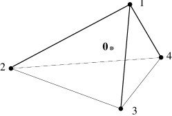
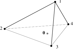
Figure 2: Self-intersection for the vertex $v_{1}$

Now we use the equation $\langle m_{234},v_{i}\rangle=a$ of the plane through the $v_{i}$ with $i=2,3,4$. Here the r.h.s. need not equal $-1$ because this plane need not bound $\Delta^{*}$. With $\langle m_{234},v_{1}\rangle=b$ we get

$$D_{1}\cdot D_{1}\cdot K3=-{a\over b}(D_{1}\cdot D_{2}\cdot K3+D_{1}\cdot D_{3}\cdot K3+D_{1}\cdot D_{4}\cdot K3).$$ (24)

Corresponding to the three different situations depicted in figure 2, we have the following possibilities: $D_{1}\cdot D_{1}\cdot K3$ is positive if 0 and $v_{1}$ are on the same side of the plane spanned by $v_{1},v_{2},v_{3}$. An example for this case is $X(\Sigma)={\mathbb{P}}^{3}$. Here $v_{1},v_{2},v_{3},v_{4}$ and 0 are the only lattice points in $\Delta^{*}$. All $D_{i}$ are linearly equivalent, so their mutual and self-intersections are equal and are easily found to be $+4$. $D_{1}\cdot D_{1}\cdot K3$ vanishes if 0 lies in the plane spanned by $v_{1},v_{2},v_{3}$ and is negative if 0 and $v_{1}$ are on different sides of this plane. In the latter case our previous arguments lead to the conclusion that we are dealing with a single rational curve of self-intersection $-2$. The same argument would apply with more than three neighbors of $v_{1}$ as long as they are in a plane. Other self-intersections of divisors corresponding to vertices with more edges originating from them can be calculated by similar means.

Let us summarize the results of this section: A divisor $D$ of the ambient space corresponding to a point $v$ of the polyhedron $\Delta^{*}$ does not intersect the $K3$ hypersurface if $v$ lies in the interior of a facet of $\Delta^{*}$. Mutual intersections of divisors $D_{1}$ and $D_{2}$ are nonzero if and only if the corresponding points $v_{1}$ and $v_{2}$ are neighbors along an edge $\theta^{*}$ of $\Delta^{*}$. In that case the intersection number is equal to the length $l$ (in lattice units) of the dual edge $\theta$ in $\Delta$. Self-intersections of divisors corresponding to points interior to edges are equal to $-2l$, where $l$ is again the length of the dual edge. If $l>1$, such a divisor must be reducible. Self-intersections of divisors corresponding to vertices are positive in the first case of figure 2. They are 0 in the second case; here we are dealing with elliptic curves. Finally, they are equal to $-2$ in the third case; this is the case of a rational curve.

4 Elliptic $K3$ Surfaces

4.1 Toric description of fibrations

Now we turn our attention to $K3$ surfaces that are elliptic fibrations. As shown in [29, 30], this means that we have a distinguished direction in the $M$ lattice, given by a primitive vector $m_{\rm fiber}$, which determines a distinguished linear hyperplane

$$N_{\rm fiber}=\{y\in N:\langle y,m_{\rm fiber}\rangle=0\}$$ (25)

in the $N$ lattice such that

$$\Delta^{*}_{\rm fiber}:=\Delta^{*}\cap N_{\rm fiber}$$ (26)

is reflexive. $N_{\rm fiber}$ divides $\Delta^{*}$ into an ‘upper’ and a ‘lower’ half to which we will refer as ‘top’ and ‘bottom’, respectively. The base space of the fibration is a ${\mathbb{P}}_{1}$ with homogeneous coordinates $(z_{\rm upper}:z_{\rm lower})$, where

$$z_{\rm upper}~{}~{}=\prod_{i:\langle v_{i},m_{\rm fiber}\rangle>0}z_{i}^{\langle v_{i},m_{\rm fiber}\rangle},~{}~{}~{}~{}~{}~{}~{}~{}~{}z_{\rm lower}~{}~{}=\prod_{i:\langle v_{i},m_{\rm fiber}\rangle<0}z_{i}^{-\langle v_{i},m_{\rm fiber}\rangle}.$$ (27)

So the linear equivalence class of the fiber is given by

$$D_{\rm fiber}~{}~{}\sim\sum_{i:\langle v_{i},m_{\rm fiber}\rangle>0}{\langle v_{i},m_{\rm fiber}\rangle}D_{i}~{}~{}~{}\sim~{}~{}~{}-\sum_{i:\langle v_{i},m_{\rm fiber}\rangle<0}{\langle v_{i},m_{\rm fiber}\rangle}D_{i}.$$ (28)

Given this, it is easy to check that the self-intersection of the generic fiber as well as the intersections of the generic fiber with any component of one of the exceptional fibers are zero. What about the self-intersections of the exceptional fibers? Self-intersections of divisors corresponding to interior points of edges are of course always negative. In all other cases we are dealing with vertices. If there is only one upper point, this point simply corresponds to the fiber without being exceptional; this is in agreement with our above analysis (self-intersection of a divisor corresponding to a point whose neighbors form a plane that contains 0). Let us now consider a vertex that is not the only upper point. At least when there are only three neighbors, they will form a plane that lies between the vertex we are considering and 0, implying a self-intersection of $-2$.

4.2 Weierstrass fibers

Specializing further, we now assume that $\Delta^{*}_{\rm fiber}$ is a triangle spanned by three vectors $v_{x}$, $v_{y}$ and $v_{z}=-2v_{x}-3v_{y}$ that generate $N_{\rm fiber}$. Our toric variety will then be described by coordinates

$$(x,y,z,z_{1},\ldots)\sim(\lambda^{2}x,\lambda^{3}y,\lambda z,z_{1},\ldots),$$ (29)

and the $K3$ surface is determined by a polynomial of degree 6 in $\lambda$. With the usual redefinitions this polynomial can be chosen as the Weierstrass polynomial in $x,y,z$ with coefficients that are functions of $z_{1},\ldots$. We also assume that $v_{z}$ lies in an edge of $\Delta^{*}$, and that its neighbors along this edge are the points $v_{a}$ ‘above’ and $v_{b}$ ‘below’ $v_{z}$, with $\langle v_{a},m_{\rm fiber}\rangle=1$, $\langle v_{b},m_{\rm fiber}\rangle=-1$. This ensures, among other things, that the points interior to the edges of the triangle $v_{x}v_{y}v_{z}$ are also interior to faces of $\Delta^{*}$, so we can disregard them in the following analysis. If there is no correction term, the Picard lattice is generated by the divisors corresponding to points of $\Delta^{*}$ that do not lie on a facet modulo three relations of linear equivalence. We may choose as the basis for the Picard lattice the following divisors:

$$D_{\rm fiber},~{}~{}~{}~{}D_{\rm section}={D_{z}},~{}~{}~{}~{}\{D_{z_{i}}\}\setminus\{D_{a},D_{b}\}.$$ (30)

It is easily checked that this is a good basis (for example, one may use linear equivalence to eliminate $D_{x},D_{y},D_{a}$ and trade $D_{\rm fiber}$ for $D_{b}$). The divisors in this basis can be grouped into three distinct sets with intersections only among members of the same set: The first one is the system $\{D_{\rm fiber},D_{\rm section}\}$ with

$$D_{\rm fiber}\cdot D_{\rm fiber}=0,~{}~{}~{}D_{\rm fiber}\cdot D_{\rm section}=1,~{}~{}~{}D_{\rm section}\cdot D_{\rm section}=-2.$$ (31)

In addition there are the sets of divisors corresponding to upper points except $v_{a}$ and those corresponding to lower points except $v_{b}$. Within each of these sets, different divisors intersect if and only if they correspond to points that are connected by edges of $\Delta^{*}$.

So far we have talked only about smooth $K3$ surfaces. Let us now consider the scenario that we shrink to zero size all of the divisors except for $D_{\rm fiber}$ and $D_{\rm section}$. Thus we obtain a surface with two point singularities. Such singularities have an $ADE$ classification which is reflected in the intersection pattern of the divisors of its blow-up. But this blow-up is just our original $K3$, and its intersection pattern is given by the structure of edges. We conclude that the Dynkin diagrams of the gauge groups that appear when the exceptional fibers are blown down to points are nothing but the ‘edge diagrams’ of the upper and lower parts of $\Delta^{*}$ without $v_{a},v_{b}$, respectively.

There is a slightly different way to find the singularity type given more than one point projecting onto a given one-dimensional cone in $\Sigma_{\rm base}$. It uses the Kodaira classification of degenerations of elliptic fibrations [31]. The possible types of degenerate fibers are shown in figure 3 and the gauge groups corresponding to those fibers are presented in table 1.

Figure 3: Classification of elliptic fibers

Fiber	I0	IN	II	III	IV	I${}_{0}^{\ast}$	I${}_{N-6}^{\ast}$	IV∗	III∗	II∗
Singularity type	—	$A_{N-1}$	—	$A_{1}$	$A_{2}$	$D_{4}$	$D_{N-2}$	$E_{6}$	$E_{7}$	$E_{8}$

Table 1: The correspondence between Kodaira and $ADE$ classifications

Each line on the figure (except for the $I_{0}$ case which is a generic smooth elliptic fiber) represents a rational curve. In order for the exceptional fiber to be homologous to the generic fiber each rational curve should be taken with multiplicity indicated by the number next to it. Now notice that in our toric picture the class of the generic fiber is given by eq. (28). Interpreting the numbers $\pm\langle v_{i},m_{\rm fiber}\rangle$ as the multiplicities of rational curves and comparing them to those shown in figure 3 we can read off the type of the exceptional fiber occurring over the point $z_{\rm upper}=0$ ($z_{\rm lower}=0$) in the base. In other words, the multiplicities shown in figure 3 are nothing else than the heights of the corresponding points in the ‘top’ in our toric picture.

Let us briefly make the connection between the present description of singularities (via blowing down divisors) and the description that is more common in the physics literature, namely by choosing particular equations. Consider the case where $\Delta^{*}$ has as vertices only $v_{x}$, $v_{y}$, $v_{a}$ and $v_{b}$, i.e. where both ‘top’ and ‘bottom’ are trivial. The most general equation (up to linear redefinitions of $x,y$) that would lead to a $K3$ hypersurface is then given by

$$y^{2}=x^{3}+p_{8}(z_{a},z_{b})xz^{4}+p_{12}(z_{a},z_{b})z^{6},$$ (32)

where $p_{8}(z_{a},z_{b})$ and $p_{12}(z_{a},z_{b})$ can be arbitrary polynomials of degrees 8 and 12, respectively. Upon restriction to

$$p_{8}=\alpha z_{a}^{4}z_{b}^{4}~{}~{}~{}~{}\hbox{ and }~{}~{}~{}p_{12}=z_{a}^{5}z_{b}^{7}+\beta z_{a}^{6}z_{b}^{6}+z_{a}^{7}z_{b}^{5},$$ (33)

we get a homogeneous version of the equation considered in [16] for the description of an $E_{8}\times E_{8}$ symmetry. This can be explained in the following way: When passing from the general form of eq. (32) to that determined by (33), we restrict $\Delta$ to a smaller polyhedron $\Delta^{\prime}$. The singularity coming from considering the non-dual pair $(\Delta^{*},\Delta^{\prime})$ may be resolved by blow-ups that change $\Delta^{*}$ to $(\Delta^{\prime})^{*}$, so we can read off the singularity type we get when we restrict eq. (32) to (33) by analyzing the structure of $(\Delta^{\prime})^{*}$. Indeed, as it should be, both the top and the bottom of $(\Delta^{\prime})^{*}$ correspond to the ‘$E_{8}$ top’ that we will shortly introduce.

4.3 Examples of $ADE$ groups

The ‘tops’ for many $ADE$ series groups were constructed in [18]. There they were identified on the basis of the Hodge numbers of the resulting Calabi–Yau threefolds and of Dynkin diagrams formed by the points in the ‘tops’. Using the methods described in the present article we can calculate intersection numbers for the divisors in the corresponding elliptic $K3$ and indeed confirm the statements made in [18].

The ‘top’ corresponding to the $SU(3)$ gauge group is shown in figure 4. The extended Dynkin diagram of $SU(3)$ is formed by the three white points one level above the plane of the generic fiber (grey points). The intersection numbers between divisors in the $K3$ whose reflexive polyhedron can be formed by adding one point just below $v_{z}$ in the triangle of the generic fiber turn out to be 1 for each pair connected by an edge. The self-intersections likewise are easily shown to be $-2$ for all three points. This exactly corresponds to the occurrence of an $I_{3}$ fiber in the elliptic $K3$ leading to an enhanced $SU(3)$ gauge symmetry in space-time if the rational curves in the degenerate fiber are blown down. Note also that the three points describing the reducible fiber are all at height 1 above the triangle in precise agreement with the fact that the $I_{3}$ fiber is formed by three rational curves which should be taken with multiplicity 1 each in order for the degenerate fiber to be homologous to the generic one.

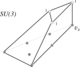
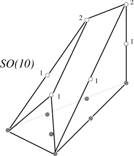
Figure 4: The ‘tops’ for $SU(3)$ and $SO(10)$. The point $v_{z}$ is shown in the $SU(3)$ picture and is the same in the following examples.

We illustrate the $D$ series case by the $SO(10)$ example shown in figure 4. There are 6 points in the ‘top’ forming an extended Dynkin diagram of $SO(10)$ (as in all the rest of our examples, we do not show the points interior to codimension one faces in the ‘tops’ since, as was explained earlier, the corresponding divisors in the ambient space do not intersect the hypersurface we are interested in). The divisors corresponding to points joined by the edges intersect with intersection number 1 for all pairs. The self-intersections found from figure 4 are all $-2$, precisely what we expect for an $I_{1}^{\ast}$ fiber. Note again that two points in the middle of the extended Dynkin diagram at hand are at height 2 above the triangle, all the rest of them being at height 1. These numbers follow exactly the multiplicities pattern shown for the $I_{1}^{\ast}$ fiber in figure 3.

The ‘tops’ corresponding to $E$ series groups are shown in figures 5 and 6. The divisors corresponding to points joined by an edge intersect and all intersection numbers are indeed found to be 1, as well as all self-intersection numbers turn out to be $-2$ revealing the intersection patterns of rational curves constituting $IV^{\ast}$, $III^{\ast}$ and $II^{\ast}$ degenerations of elliptic fibers respectively. Extended Dynkin diagrams are hence formed by those points, again confirming the observation made in [18]. The heights of the points above the plane of the triangle follow precisely the multiplicities of rational curves shown in figure 3. It is also amusing to calculate the ranks of Picard groups for the $K3$ surfaces described by the reflexive polyhedra obtained by adding a trivial ‘bottom’ (in terminology of [18]) to our ‘tops’. The application of (15) yields 8, 9 and 10 in the $E_{6}$, $E_{7}$ and $E_{8}$ cases, respectively, the correction (third) term in (15) being always zero.

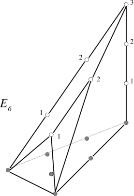
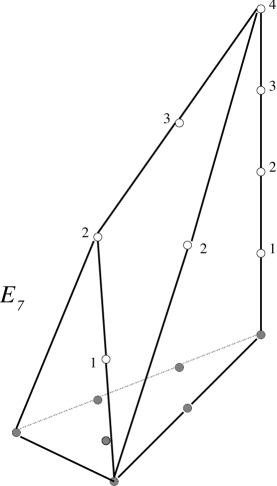
Figure 5: The ‘tops’ for $E_{6}$ and $E_{7}$

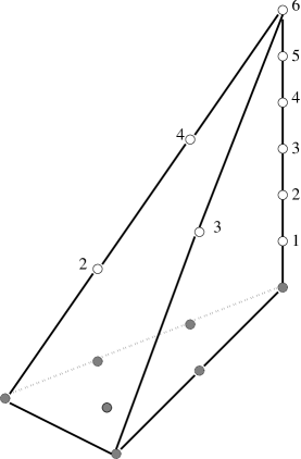
Figure 6: The ‘top’ for $E_{8}$ (the vertical scale is half of that for the rest of ‘tops’ figures)

5 Threefold Case

5.1 Toric description

In this section, we generalize the construction presented in the previous one to the case of elliptically fibered Calabi–Yau threefolds. Namely, we present an explanation of the methods used in [21] to unravel the singularity structure of elliptic Calabi–Yau threefolds given as hypersurfaces in toric varieties.

Again, as in the elliptic $K3$ case of the previous section, such a Calabi–Yau threefold being an elliptic fibration is equivalent to the existence of a two-dimensional plane $H$ in $N_{\mathbb{R}}$ such that $H\cap\Delta^{\ast}=\Delta^{\ast}_{\rm fiber}$ is a reflexive polyhedron describing the generic fiber of the elliptic fibration. This observation was first made in [18]. As was shown in [30], the base in this case can be seen by projecting the $N$ lattice along the linear space $H$ spanned by $\Delta^{\ast}_{\rm fiber}$. The projection map from $X(\Sigma)$ (four-dimensional embedding variety of the Calabi-Yau threefold, in our case) to the base was given as follows.

The set of one-dimensional cones in $\Sigma_{\rm base}$ is the set of images of one-dimensional cones in $\Sigma_{CY}$ that do not lie in $N_{\rm fiber}$. The image of a primitive generator $v_{i}$ of a cone in $\Sigma_{CY}$ is the origin or a positive integer multiple of a primitive generator $\tilde{v}_{j}$ of a one-dimensional cone in $\Sigma_{\rm base}$. Thus we can define a matrix $r^{i}_{j}$, most of whose elements are $0$, through $\pi v_{i}=r_{i}^{j}\tilde{v}_{j}$ with $r_{i}^{j}\in{\mathbb{N}}$ if $\pi v_{i}$ lies in the one-dimensional cone defined by $\tilde{v}_{j}$ and $r_{i}^{j}=0$ otherwise. Our base space is the multiply weighted space determined by

$$(\tilde{z}_{1},\ldots,\tilde{z}_{\tilde{N}})\sim(\lambda^{\tilde{w}^{1}_{j}}\tilde{z}_{1},\ldots,\lambda^{\tilde{w}^{\tilde{N}}_{j}}\tilde{z}_{\tilde{N}}),~{}~{}~{}~{}~{}~{}j=1,\ldots,\tilde{N}-\tilde{n}$$ (34)

where the $\tilde{w}^{i}_{j}$ are any integers such that $\sum_{i}\tilde{w}^{i}_{j}\tilde{v}_{i}=0$. The projection map from $X(\Sigma)$ (and also, as was demonstrated in [30], from the Calabi–Yau hypersurface) to the base is given by

$$\tilde{z}_{i}=\prod_{j}z_{j}^{r_{j}^{i}}.$$ (35)

The fiber can degenerate. There are two possible mechanisms for that. Since the fiber is a hypersurface in $X(\Sigma_{\rm fiber})$, it can happen either when the embedding variety $X(\Sigma_{\rm fiber})$ itself degenerates or the equation of the hypersurface becomes singular. As all divisors are manifest in the blown-up toric picture, the second case can only correspond to the cases $I_{1}$ or $II$ in the Kodaira classification, which do not lead to enhanced gauge groups. If a one-dimensional cone with primitive generator $\tilde{v}_{i}$ in $\Sigma_{\rm base}$ is the image of more than one one-dimensional cone in $\Sigma$, the fiber over the divisor $\tilde{D}_{i}$ determined by $\tilde{z}_{i}=0$ is reducible: different components of the fiber corresponding to equations $z_{j}=0$ project on $\tilde{D}_{i}$ whenever different cones $v_{j}$ project on one cone $\tilde{v}_{i}$ in $\Sigma_{\rm base}$.

If we take a small disk $D\subset{\mathbb{C}}$ in the base that intersects the divisor $\tilde{D}_{i}$ transversely at a generic point we can consider the picture locally near the point of intersection $p$. To determine the singularity type along the divisor $\tilde{D}_{i}$ we need to find the intersection numbers of the components of the fiber over $p$ in the two-dimensional manifold which is a fibration over $D$. To accomplish this task by our toric means we consider only the points of $\Delta^{\ast}$ which project to the one-dimensional cone in $\Sigma_{\rm base}$ corresponding to $\tilde{D}_{i}$. These points form a three-dimensional fan describing the local data we are after. Indeed, the divisor $\tilde{D}_{i}$ is given by $\tilde{z_{i}}=0$, where $\tilde{z_{i}}$ is the coordinate assigned to the one-dimensional cone corresponding to that divisor. Taking only that one-dimensional cone means that the only coordinate we are left with is $\tilde{z_{i}}$. Varying it we move in a direction in the base transverse to our divisor. What we get is in fact one of the ‘tops’ discussed in section 3, with the ‘heights’ determined by the numbers $r_{j}^{i}$. The computation of the intersections presented there carries over to the threefold case.

5.2 Monodromy and non-simply laced groups

Up until now the enhanced gauge symmetry occurring in the uncompactified dimensions coincided with the corresponding singularity type of the internal manifold. This does not have to be the case though as was first shown in [32]. It is indeed so provided the rational curves within the exceptional fiber are monodromy invariant as we move around the corresponding curve within the base. In the cases when those curves are not monodromy invariant, the gauge group appearing in space-time is actually a subgroup invariant under the outer automorphism obtained by translating the monodromy action on the rational curves into an action on the Dynkin diagrams of the simply-laced gauge group corresponding to the singularity type. The possible outer automorphisms and their actions on the Dynkin diagrams are shown in figure 7.

Figure 7: Outer automorphisms of Lie algebras

What happens from the toric point of view is the following. If there is a monodromy action on the rational curves in the fiber over a point $p$ then several divisors in the $K3$ which are exchanged by the monodromy action yield only one divisor in the Calabi–Yau threefold when transported over the whole of $\tilde{D}_{i}$, the divisor in the base. Hence, they are represented by just one point in the polar polyhedron $\Delta^{\ast}$ of the Calabi–Yau threefold. In the complex surface which is a fibration over the disk $D$, that point in $\Delta^{\ast}$ (when regarded as a point in the particular ‘top’, the inverse image of the cone $\tilde{v}_{i}$ in $\Sigma_{\rm base}$) corresponds to several divisors or, more precisely, to their sum. Hence, the self-intersection of the divisor class represented by this particular point in the ‘top’ should turn out to be $-2m$, where $m$ is the number of rational curves identified under the monodromy. One more point is worth mentioning. By inspection of figures 3 and 7, we can convince ourselves that the rational curves exchanged by a monodromy always have equal multiplicity. Hence the points representing the divisor classes of their sum should have the height in the corresponding ‘tops’ equal to that multiplicity. We will see that this is indeed the case in the examples below.

5.3 Examples of non-simply laced groups

5.3.1 $SO(2n+1)$

An $SO(2n+1)$ gauge group appears as a result of a monodromy action on $I_{n-3}^{\ast}$ fibers which exchanges two rational curves leading to only one divisor in the Calabi–Yau threefold when transported over the divisor in the base of the elliptic fibration. Thus these two rational curves are represented by one point in the polyhedron $\Delta^{\ast}$. This point when regarded as a point in the corresponding ‘top’ represents the sum of the two rational curves exchanged by the monodromy. Thus the self-intersection of the divisor class should be $-4$. The intersection number between this divisor class and the divisor class corresponding to the point in the Dynkin diagram of $SO(2n+2)$ connected to the two points exchanged by the outer automorphism equals $1+1=2$. The remaining intersections involve simply rational curves and should be equal to $-2$ for self-intersections and 1 for mutual ones. As an illustration to this case, we depict the ‘top’ corresponding to the gauge group $SO(9)$ in figure 8. The self-intersection number calculated for the black dot in the figure is $-4$ and the intersection number between the black dot and the white one connected to it by an edge is 2. The other self-intersections are $-2$ as expected. The heights of the white points are exactly as in $SO(10)$ case. The height of the black point is 1 since the multiplicities of the rational curves in the $I_{1}^{\ast}$ fiber exchanged by the monodromy are 1. As always, the extended Dynkin diagram of $SO(9)$ is visible in the ‘top’. The $K3$ polyhedron obtained by adding one point just below $v_{z}$ has Picard number 6, in agreement with the presence of an $SO(10)$ lattice in the Picard lattice.

5.3.2 $Sp(n)$

In order to obtain $Sp(n)$ symmetry in space-time we need a curve of $SU(2n)$ singularities in our Calabi–Yau threefold, or, in other words, a divisor in the base with $I_{2n}$ fibers over it subject to a monodromy action. The pairs of curves exchanged by the monodromy will produce only one divisor in the Calabi–Yau each when transported over the divisor in the base. Hence, in our complex surface which is a fibration over the small disk $D$, the divisor classes of the sums of the rational curves identified under the monodromy will be represented by points in $\Delta^{\ast}$ of the Calabi–Yau threefold. That is, we expect $n+1$ relevant points in the corresponding ‘top’, $n-1$ of them with self-intersection $-4$ and all mutual intersections equal to 2. The self-intersections for the remaining two points are $-2$, each of them representing only one rational curve in the complex surface. We illustrate this case by an $Sp(3)$ ‘top’ found in [18]. It is shown in figure 8. As before, the points in the subpolyhedron of the generic fiber are shown in grey color. All the relevant points are white and black, the black ones corresponding to sums of the rational curves identified under the monodromy. All the multiplicities in $I_{6}$ fibers are one. Hence the heights of all points in the $Sp(3)$ ‘top’ should be 1. We see that this is indeed the case. The extended Dynkin diagram of $Sp(3)$ is clearly visible and appears in a natural fashion. As an additional check, note that adding one point below the point $v_{z}$ we obtain a reflexive polyhedron of a $K3$ surface whose Picard number equals 7, in agreement with the presence of an $SU(6)$ gauge group (which gives $Sp(3)$ under the outer automorphism action).

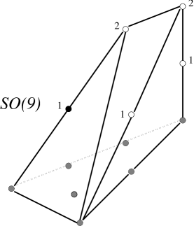
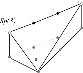
Figure 8: The ‘tops’ for the gauge groups $SO(9)$ and $Sp(3)$.

5.3.3 $F_{4}$

When the monodromy acts on a curve of $IV^{\ast}$ fibers $F_{4}$ gauge symmetry results. Two pairs of rational curves are exchanged under this monodromy leading to two points in the Calabi–Yau threefold which describe divisor classes in the complex surface with self-intersections of $-4$. The self-intersection of the remaining three rational curves in the $IV^{\ast}$ fiber we expect to be simply $-2$. The mutual intersections involving divisor classes of sums of rational curves are easily seen to be 2, and 1 otherwise. This is exactly what we calculated in the $F_{4}$ ‘top’ shown in figure 9. As before, black dots represent the sums of rational curves and white ones rational curves forming the extended Dynkin diagram of $F_{4}$. Note also that the heights of the points shown in the figure are exactly as in the $E_{6}$ case except for the fact that two white points of height 2 and two white points of height 1 are replaced by one black point of the same height, respectively, following the monodromy action on the rational curves. As in the previous case, we can construct a reflexive polyhedron of a $K3$ by adding one point to the ‘top’. The Picard number of this $K3$ turns out to be 8, as we could expect.

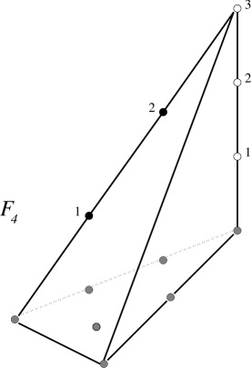
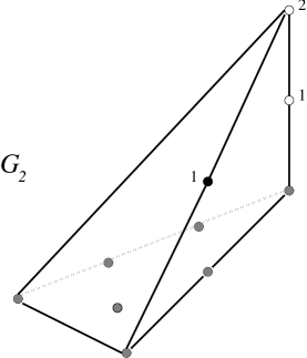
Figure 9: The ‘tops’ for $F_{4}$ and $G_{2}$

5.3.4 $G_{2}$

$G_{2}$ gauge symmetry is a result of a monodromy action on a curve of $I_{0}^{\ast}$ fibers. Under this monodromy three rational curves are exchanged, so we expect the divisor class of their sum to be represented by one point in the corresponding Calabi–Yau threefold. The self-intersection of this divisor class we expect to be $-6$. Correspondingly, the intersection number between this divisor class and the divisor which is invariant under the monodromy should be 3. The intersection between the latter and another such (the one which corresponds to the extending point in the extended Dynkin diagram of $G_{2}$) should be 1. Of course the self-intersections of the latter two are $-2$ as they represent rational curves. The ‘top’ corresponding to $G_{2}$ is shown in figure 9. The black dot represents the sum of three rational curves. The $I_{0}^{\ast}$ fiber has one rational curve with multiplicity 2. It is invariant under the monodromy. Hence there is one white point of height 2 in our ‘top’. The three curves exchanged by the monodromy all have multiplicity 1. The black dot is at height 1 in agreement with that. The extended Dynkin diagram of $G_{2}$ is again clearly visible. By adding one point below $v_{z}$ we obtain the reflexive polyhedron of the $K3$. The calculation of the Picard number gives 6, in agreement with the presence of $SO(8)$ in the Picard lattice.

6 Discussion

In this article we have given a systematic exposition of methods allowing one to read off the singularity structure of Calabi–Yau manifolds described as hypersurfaces in toric varieties. We particularly focused on the cases leading to enhanced gauge symmetries in F-theory (or type II) compactifications. These methods have already been used in the literature [18, 21] but an explanation was lacking. We have shown that $ADE$ orbifold singularities of a toric $K3$ surface (upon their resolution) exhibit themselves in the form of extended Dynkin diagrams of corresponding simply laced Lie groups appearing in the reflexive polyhedra, the fact noticed and used in [18]. These are precisely the groups observed in the low energy spectrum of the corresponding compactified theory. Moreover, we have shown that a nontrivial monodromy action in the case of a Calabi–Yau threefold with curves of singularities leading to the appearance of non-simply laced groups is also encoded in the corresponding polyhedra in a rather simple fashion. As also was noticed in [18], the extended Dynkin diagram of a simply laced group (the singularity type along the curve) undergoes just the right outer automorphism to yield the extended Dynkin diagram of the non-simply laced group which is observed in the effective theory.

These methods, though discussed in the case of elliptic Calabi–Yau threefolds carry over without any major changes to the elliptic fourfold case (and, in principle, to $n$-folds with $n>4$). Each ray in the fan of the base represents a divisor and the points of the polyhedron projecting on a given ray encode the way the elliptic fiber degenerates over that divisor. One more remark is in order. The methods we described and explained apply to the cases in which the singularity structure of a threefold (or $n$-fold) can be analyzed in terms of that of a complex surface, i.e. it is enough to consider a small disc $D\in{\mathbb{C}}$ (or $D\in{\mathbb{C}}^{n-2}$) cutting the divisor in the base transversely and analyze the geometry of the complex surface which is a fibration over $D$. There are cases which cannot be reduced to that and which are encountered in string theory. We think that torically one of the signs of such cases is the fact that the points irrelevant in the corresponding ‘top’ become relevant in the polyhedron of the threefold. It would be interesting to find a systematic toric way of analyzing such more complicated cases.

Acknowledgements: We would like to thank P. Candelas, S. Katz and G. Rajesh for useful discussions. This work was supported by the Austrian “Fonds zur Förderung der wissenschaftlichen Forschung” with a Schrödinger fellowship, number J012328-PHY, NSF grant PHY-9511632 and the Robert A. Welch Foundation.

References

- [1]
- [2]
- [3]
- [4] C. Hull and P. Townsend, Unity of Superstring Dualities, Nucl. Phys.B438 (1995) 109, hep-th/9410167.
- [5] E. Witten, String Theory Dynamics in Various Dimensions, Nucl. Phys.B443 (1995) 85, hep-th/9503124.
- [6] A. Strominger, Massless Black Holes and Conifolds in String Theory, Nucl. Phys. B451 (1995) 96, hep-th/9504090.
- [7] P.S. Aspinwall, An Dual Pair and a Phase Transition, Nucl. Phys. B460 (1996) 57, hep-th/9510142.
- [8] M. Bershadsky, V. Sadov and C. Vafa, D-Strings on D-Manifolds, Nucl. Phys. B463 (1996) 398, hep-th/9510225.
- [9] P.S. Aspinwall, Enhanced Gauge Symmetries and Calabi-Yau Threefolds, Phys. Lett. B371 (1996) 231, hep-th/9511171.
- [10] S. Katz, D.R. Morrison and M.R. Plesser, Enhanced Gauge Symmetry in Type II String Theory, Nucl. Phys. B477 (1996) 105 hep-th/9601108.
- [11] S. Kachru and C. Vafa, Exact Results for N=2 Compactifications of Heterotic Strings, Nucl. Phys. B450 (1995) 69, hep-th/9505105.
- [12] A. Klemm, W. Lerche and P. Mayr, K3–Fibrations and Heterotic-Type II String Duality, Phys. Lett. B357 (1995) 313, hep-th/9506112.
- [13] P.S. Aspinwall and J. Louis, On the Ubiquity of Fibrations in String Duality, Phys. Lett. B369 (1996) 233, hep-th/9510234.
- [14] C. Vafa, Evidence for F-Theory, Nucl. Phys. B469 (1996) 403, hep-th/9602022.
- [15] D.R. Morrison and C. Vafa, Compactifications of F-Theory on Calabi–Yau Threefolds – I, Nucl. Phys. B473 (1996) 74, hep-th/9602114.
- [16] D.R. Morrison and C. Vafa, Compactifications of F-Theory on Calabi–Yau Threefolds – II, Nucl. Phys. B476 (1996) 437, hep-th/9603161.
- [17] M. Bershadsky, K. Intriligator, S. Kachru, D. R. Morrison, V. Sadov, C. Vafa, Geometric Singularities and Enhanced Gauge Symmetries, Nucl. Phys. B481 (1996) 215, hep-th/9605200.
- [18] P. Candelas and A.Font, Duality Between the Webs of Heterotic and Type II Vacua, hep-th/9603170, revised version (march 1997).
- [19] P. Candelas, E. Perevalov and G. Rajesh, F-Theory Duals of Nonperturbative Heterotic Vacua in Six Dimensions, hep-th/9606133.
- [20] P. Candelas, E. Perevalov and G. Rajesh, Comments on A,B,C Chains of Heterotic and Type II Vacua, hep-th/9703148.
- [21] P. Candelas, E. Perevalov and G. Rajesh, Toric Geometry and Enhanced Gauge Symmetry of F-Theory/Heterotic Vacua, hep-th/9704097, .
- [22] A. Klemm and P. Mayr, Strong Coupling Singularities and Non-abelian Gauge Symmetries in String Theory, hep-th/9601014.
- [23] S. Katz, A. Klemm and C. Vafa, Geometric Engineering of Quantum Field Theories, hep-th/9609239.
- [24] W. Fulton, Introduction to Toric Varieties (Princeton Univ. Press, Princeton 1993).
- [25] T. Oda, Convex Bodies and Algebraic Geometry (Springer, Berlin Heidelberg 1988).
- [26] D. Cox, The Homogeneous Coordinate Ring or a Toric Variety, J. Alg. Geom. 4 (1995) 17.
- [27] V.V.Batyrev, Dual polyhedra and mirror symmetry for Calabi–Yau hypersurfaces in toric varieties, J. Alg. Geom. 3 (1994) 493, alg-geom/9310003.
- [28] P.Candelas, X. de la Ossa, S.Katz, Mirror symmetry for Calabi–Yau hypersurfaces in weighted and extensions of Landau–Ginzburg theory, Nucl. Phys. B450 (1995) 267, hep-th/9412117.
- [29] A. Avram, M. Mandelberg, M. Kreuzer and H. Skarke, Searching for Fibrations, hep-th/9610154.
- [30] M. Kreuzer and H. Skarke, Calabi–Yau Fourfolds and Toric Fibrations, hep-th/9701175.
- [31] K. Kodaira, On Compact Analytic Surfaces II, Ann. Math. 77 (1963) 563 .
- [32] P.S. Aspinwall and M. Gross, The SO(32) Heterotic String on a Surface, Phys. Lett. B387 (1996) 735.