Theoretical Physics Institute
University of Minnesota

TPI-MINN-97/09-T

UMN-TH-1535-97

hep-th/9704114

Non-Perturbative Dynamics in Supersymmetric Gauge Theories

Extended version of lectures given at International School of Physics “Enrico Fermi”, Varenna, Italy, July 3 - 6, 1995, Institute of Nuclear Science, UNAM, Mexico, April 11 - 17, 1996, and Summer School in High-Energy Physics and Cosmology, 10 - 26 July, 1996, ICTP, Triest, Italy.

M. Shifman

Theoretical Physics Institute, Univ. of Minnesota, Minneapolis, MN 55455

I give an introductory review of recent, fascinating developments in supersymmetric gauge theories. I explain pedagogically the miraculous properties of supersymmetric gauge dynamics allowing one to obtain exact solutions in many instances. Various dynamical regimes emerging in supersymmetric Quantum Chromodynamics and its generalizations are discussed. I emphasize those features that have a chance of survival in QCD and those which are drastically different in supersymmetric and non-supersymmetric gauge theories.

Unlike most of the recent reviews focusing almost entirely on the progress in extended supersymmetries (the Seiberg-Witten solution of $N=2$ models), these lectures are mainly devoted to $N=1$ theories. The primary task is extracting lessons for non-supersymmetric theories.

1 Lecture 1. Basic Aspects of Nonperturbative Gauge Dynamics

1.1 Introduction

All fundamental interactions established in nature are described by non-Abelian gauge theories. The standard model of the electroweak interactions belongs to this class. In this model, the coupling constant is weak, and its dynamics is fully controlled (with the possible exception of a few, rather exotic problems, like baryon number violation at high energies).

Another important example of the non-Abelian gauge theories is Quantum Chromodynamics (QCD). This theory has been under intense scrutiny for over two decades, yet remains mysterious. Interaction in QCD becomes strong at large distances. What is even worse, the degrees of freedom appearing in the Lagrangian (microscopic variables – colored quarks and gluons in the case at hand) are not those degrees of freedom that show up as physical asymptotic states (macroscopic degrees of freedom – colorless hadrons). Color is permanently confined. What are the dynamical reasons of this phenomenon?

Color confinement is believed to take place even in pure gluodynamics, i.e. with no dynamical quarks. Adding massless quarks produces another surprise. The chiral symmetry of the quark sector, present at the Lagrangian level, is spontaneously broken (realized nonlinearly) in the physical amplitudes. Massless pions are the remnants of the spontaneously broken chiral symmetry. What can be said, theoretically, about the pattern of the spontaneous breaking of the chiral symmetry?

Color confinement and the spontaneous breaking of the chiral symmetry are the two most sacred questions of strong non-Abelian dynamics; and the progress of understanding them is painfully slow. At the end of the 1970s Polyakov showed that in 3-dimensional compact electrodynamics (the so called Georgi-Glashow model, a primitive relative of QCD) color confinement does indeed take place [1]. Approximately at the same time a qualitative picture of how this phenomenon could actually happen in 4-dimensional QCD was suggested by Mandelstam [2] and ’t Hooft [3]. Some insights, though quite limited, were provided by models of the various degree of fundamentality, and by numerical studies on lattices. This is, basically, all we had before 1994, when a significant breakthrough was achieved in understanding both issues in supersymmetric (SUSY) gauge theories.

Unlike the Georgi-Glashow model in three dimensions mentioned above, which is quite a distant relative of QCD, four-dimensional supersymmetric gluodynamics and supersymmetric gauge theories with matter come much closer to genuine QCD. Moreover, the dynamics of these theories is rich and interesting by itself, which accounts for the attention they have attracted in the last two or three years. Although the development is not yet complete, the lessons are promising, and definitely deserve thorough studies. Several topics which I consider to be most interesting are discussed below in this lecture course. Before submerging into supersymmetry proper, however, it is worth reiterating the main general ideas which are the key players in this range of questions: the Meissner and the dual Meissner effects, monopoles, Abelian projection of QCD, and so on. The first part is a brief review of these issues intended mostly to refresh the memory and to provide a representative list of pedagogical literature. We will start an excursion into supersymmetric gauge theories in Sect. 2, and gradually proceed from simpler topics to more complicated ones. The simplest supersymmetric non-Abelian model is SUSY gluodynamics. Simultaneously, it happens to be the closest approximation to QCD (without light quarks). Although there was essentially no progress towards the solution of this theory the seeds of the miraculous properties of the supersymmetric gauge dynamics are clearly visible. I will explain how some exact results (the first example ever in four-dimensional strongly coupled field theory!) can be derived. These results will become a part of our tool kit used in revealing various dynamical scenarios in SUSY gauge theories with matter.

In Sect. 3 we will open a fascinating world of supersymmetric $SU(N_{c})$ QCD, a world populated by a variety of unusual regimes governed by nonperturbative supersymmetric dynamics. Here, among other rarities, we will find confinement without spontaneous chiral symmetry breaking, with spontaneous breaking of the baryon number; the so called $s$-confinement, with additional composite massless fields not related to Goldstone modes of the spontaneously broken global symmetries. We will discover a conformal window – a set of pairs of theories with different gauge groups but identical global symmetries that are dual (equivalent) to each other as far as infrared behavior is concerned. The infrared asymptotics of these theories is (super)conformal. Outside the conformal window we will encounter dual pairs, with one theory coupled superstrongly and another free in the infrared domain. The gauge bosons of the latter can be considered as composite superstrongly bound states in the former theory.

Section 4 is a very brief travel guide to the supersymmetric gauge theories with other gauge groups. New phenomena we will encounter are the so called oblique confinement and triality – the infrared equivalence of three distinct theories. One of them is in the Higgs phase, another in the confinement phase, and the third one is in the oblique confinement phase.

Finally, in Sect. 5, supersymmetry is explicitly (softly) broken by the gluino and squark masses. Ideally, we would like to send these masses to infinity, evolving towards non-supersymmetric theories, without loosing our calculational abilities. Unfortunately, once the gluino and squark masses become large enough, the calculational abilities are lost. We have to settle for small perturbations of the supersymmetric solution. By exploring the dynamical properties of the theory obtained in this way one hopes to get qualitative insights about what happens in the limit of infinitely heavy squarks and gluino.

This review is an extended version of my lecture notes. The pedagogical style of presentation is preserved, where possible. Simple and general issues are discussed first, providing a necessary background for more advanced theoretical constructions and conclusions. Occasional remarks intended for expert readers will slip, though; they may be ignored in the first reading.

1.2 Phases of gauge theories (Abelian version)

Quantum electrodynamics (QED) was historically the first gauge theory studied in detail. Although from the modern perspective it seems to be a very simple model, with no mysteries, it can exhibit at least three different types of behavior. Let us consider supersymmetric version, SQED. The Lagrangian of the model is [4]

$${\cal L}=-\frac{1}{4}F_{\mu\nu}^{2}+\bar{\psi}i\not\!\!D\psi-m\bar{\psi}\psi+$$

$$(D_{\mu}\phi)^{\dagger}(D_{\mu}\phi)-m^{2}\phi^{\dagger}\phi+(D_{\mu}\chi)^{\dagger}(D_{\mu}\chi)-m^{2}\chi^{\dagger}\chi-$$

$$\frac{e^{2}}{2}(\phi^{\dagger}\phi-\chi^{\dagger}\chi)^{2}+$$

$$\frac{i}{2}\bar{\lambda}\not\!\partial\lambda+e\left\{\bar{\lambda}\frac{1+\gamma^{5}}{2}\psi\phi^{\dagger}+\bar{\lambda}\frac{1-\gamma^{5}}{2}\psi\chi+\mbox{h.c.}\right\}\,,$$ (1.1)

where $\phi$ and $\chi$ are complex scalar fields with the charges $+e$ and $-e$, respectively, (selectrons), and $\lambda$ is the photino (Majorana) field. The first line in Eq. (1.1) is just conventional quantum electrodynamics of photons and electrons, the second line gives the kinetic and the mass terms of electron’s superpartners, selectrons, the third line is the selectron self-interaction, and, finally, the fourth line presents the photino kinetic term and photino’s interactions. As we will see later, supersymmetry guarantees that the overall form of the Lagrangian is preserved under quantum corrections – no new counterterms appear.

Assume first that the electron and selectron mass (they are the same) does not vanish, and $\alpha\equiv e^{2}/4\pi\ll 1$. For $m\neq 0$ the vacuum state of the theory is unique; it corresponds to the vanishing expectation values of the scalar fields, $\langle\phi\rangle=\langle\chi\rangle=0$. Apart from the fact that some of the charged particles have spin zero, the theory is very much like QED. If heavy (static) probe charges are introduced, their interaction is just Coulomb, with the potential proportional to

$$V(R)\sim\frac{\alpha(R)}{R}$$

where $R$ is the distance between the probe charges. Classically $\alpha$ is constant, of course, but quantum renormalization makes $\alpha$ run. The behavior of $\alpha$ is determined by the well-known Landau formula. At large distances $\alpha$ decreases logarithmically; if $m$ is finite, however, the logarithmic fall off is frozen at $R\sim m^{-1}$; the corresponding critical value of $\alpha$ is $\alpha_{*}=\alpha(R=m^{-1})$. The potential between the distant static charges is

$$V(R)\sim\frac{\alpha_{*}}{R}\,,\,\,\,\,R\rightarrow\infty\,.$$ (1.2)

The dynamical regime with this type of the long-distance behavior is referred to as the Coulomb phase. In the case at hand we deal with the Abelian Coulomb phase. Similar behavior, Eq. (1.2), can take place in the non-Abelian gauge theories as well. Non-Abelian gauge theories with the long-range potential (1.2) are said to be in the non-Abelian Coulomb phase.

What happens if the mass parameter $m$ is set equal to zero? Note, that in SUSY theories, if the bare value of $m$ is fine-tuned to vanish, it will remain at zero with all quantum corrections.

The most drastic change is evident at first glance, after examining the third line in Eq. (1.1). The minimum of the potential energy is achieved now not only at the vanishing values of the scalar fields but, rather, on a one-dimensional complex manifold. Indeed, $\phi$ can be arbitrary complex number; if $\phi=\chi$ the potential energy obviously vanishes. The continuous degeneracy of the classical minimal-energy state (the so called vacuum valley) is a rather typical feature of supersymmetric theories with matter. We will return to the in-depth discussion of this aspect later.

Quantum-mechanically one can say that the expectation value $\langle\phi\chi\rangle\neq 0$ may take arbitrary complex value; here $\phi\chi$ is a convenient gauge invariant product parametrizing the vacuum valley. If the scalar fields $\phi$ and $\chi$ take constant non-vanishing values in the vacuum, the Higgs phenomenon takes place [5]: the gauge symmetry ($U(1)$ in the case at hand) is spontaneously broken.

What does one mean by saying that the gauge symmetry is spontaneously broken? The gauge symmetry, in a sense, is not a symmetry at all – rather, it is a description of $x$ physical degrees of freedom in terms of $x+y$ variables; $y$ variables are redundant; the corresponding degrees of freedom are physically unobservable. In other words, only a subspace of all field space ($\psi,\bar{\psi},\phi,\phi^{\dagger},\chi,\chi^{\dagger},A_{\mu}$ in the model under consideration), corresponding to gauge non-equivalent points, describe physically observable degrees of freedom.

Let us first switch off the electric charge, $e=0$. Then the Lagrangian (1.1) is invariant under the global phase rotations, $\phi\rightarrow e^{i\alpha}\phi$, $\chi\rightarrow e^{-i\alpha}\chi$, $\psi\rightarrow e^{i\alpha}\psi$. The condensation of the scalar fields breaks this invariance. But invariance of the model is not lost. Under the phase transformation one vacuum goes into another, physically equivalent. Say, if we start from the vacuum characterized by a real value of the order parameter $\phi$ and $\chi$, in the “rotated” one the order parameter is complex. The spontaneous breaking of any global symmetry leads to a set of degenerate (and physically equivalent) vacua.

If we now switch on the photons, ($e\neq 0$), the degeneracy associated with the spontaneous breaking of the global symmetry is gone. All states related by the phase rotation are gauge-equivalent, and only one of them should be left in the Hilbert space of the theory. In other words, one can always choose the vacuum values of $\phi$ and $\chi$ to be real. This is nothing but the gauge condition. Thus, spontaneous breaking of the gauge symmetry does not imply, generally speaking, the existence of a degenerate set of vacua, as is the case with the global symmetries. Then, what does it mean, after all?

By inspecting Lagrangian (1.1) it is not difficult to see that if $\phi$ and $\chi$ have non-vanishing (and constant) values in the vacuum, the spectrum of the theory does not contain massless vector particles at all. The photon acquires mass, $M_{V}^{2}=4e^{2}|v|^{2}$, where $v^{2}=\langle\phi\chi\rangle$, through the mixing with the “phases” of the fields $\phi$ and $\chi$. In the supersymmetric model considered, we “cook” in this way a massive vector field and a massive (real) scalar field, both with masses $M_{V}$, and a massless complex scalar field, out of massless photon and two massless complex scalar fields. (All these boson fields are accompanied by their fermion superpartners, of course).

This regime is referred to as the Higgs phase. One massless scalar field is eaten up by the photon field in the process of the transition to the Higgs phase. In the Higgs phase the electric charge is screened by the vacuum condensates. If we put a probe (static) electric charge in the vacuum, the Coulomb potential $\sim 1/R$ it induces at short distances (i.e. distances less than $M_{V}^{-1}$) gives place to the Yukawa potential $\sim\exp(-M_{V}R)/R$ at distances larger than $M_{V}^{-1}$. The gauge coupling runs, according the standard Landau formula, only at distances shorter than $M_{V}^{-1}$, and is frozen at $M_{V}^{-1}$.

There is one single point in the vacuum valley, the origin, (i.e. $\langle\phi\chi\rangle=0$) where the gauge symmetry is unbroken. The long-range force due to massless photons is not screened by the vacuum condensates of the scalar fields. A different type of screening does occur, however, due to quantum effects. Indeed, the photon propagator is dressed by the virtual pairs of electrons and selectrons. This dressing results in the running of the effective charge $\alpha(R)$,

$$\alpha(R)\sim\frac{1}{\ln R}\,.$$ (1.3)

Unlike the massive case, where this running is frozen at $R=m^{-1}$, in the theory with $m=0$ (and $\langle\phi\chi\rangle=0$) the logarithmic fall off (1.3) continues indefinitely: at asymptotically large $R$ the effective coupling becomes asymptotically small.

Thus, the asymptotic limit of massless QED is a free photon (and photino) plus massless matter fields whose charge is completely screened. The theory does not have localized asymptotic states and no mass shell at all, no $S$ matrix in the usual sense of this word. Still, it is well-defined in finite volume.

This phase of the theory is referred to as a free phase. Sometimes it is also called the Landau zero-charge phase. Strictly speaking, the model is ill-defined at short distances where the effective coupling grows and finally hits the Landau pole. To make it self-consistent, at short distances it must be embedded into an asymptotically free theory. This is not difficult to achieve. The Georgi-Glashow model gives an example of such an embedding.

Summarizing, even in the simplest Abelian example we encounter three different phases, or dynamical regimes: the Coulomb phase, the Higgs phase and the free (Landau) phase, depending on the values of parameters of the model and the choice of the vacuum state (in the case of the vanishing mass parameter, $m=0$). All these regimes are attainable in non-Abelian models too. The non-Abelian gauge theories are richer, however, since they admit one more dynamical regime, confinement of color, a famous property of QCD which attracted so much attention but still defies analytic solution.

1.3 Non-Abelian Higgs model; monopoles

Interactions of quarks and leptons at the fundamental level are described by non-Abelian gauge theories. The standard model of electroweak interactions is, probably, the most well-studied non-Abelian gauge theory in the Higgs phase. Apart from a few exotic phenomena (e.g. the baryon number violation at high energies, for reviews see [6]) all processes in this model occur in the weak coupling regime, and are well-understood. The dynamical content is almost exhausted by perturbation theory; very small nonperturbative corrections are due to instantons.

Since this model is so well-studied and familiar to everybody, it makes more sense to discuss another example of a non-Abelian Higgs phenomenon, the Georgi-Glashow model [7]. This example is instructive and more relevant to the discussion below since this model exhibits magnetic monopoles [8]. A nice review of the Georgi-Glashow model, with special emphasis on this particular aspect, magnetic monopoles and dyons, can be found in Ref. [9].

The gauge group of the model is $SU(2)$, so it has three gauge bosons. The matter sector includes one real scalar field $\phi^{a}$ in the adjoint representation of $SU(2)$ (i.e. $a=1,2,3$). The Lagrangian has the form

$${\cal L}=-\frac{1}{4}G_{\mu\nu}^{a}G_{\mu\nu}^{a}+\frac{1}{2}(D_{\mu}\phi^{a})(D_{\mu}\phi^{a})-\frac{1}{4}\lambda(\phi^{a}\phi^{a}-v^{2})^{2}$$ (1.4)

where $\lambda$ is a scalar coupling constant, and $v$ is a constant of dimension of mass determining the vacuum expectation value of the $\phi$ field. The so-called Bogomol’nyi-Prasad-Sommerfield (BPS) limit [10, 11]

$$\lambda\rightarrow 0\,,\,\,\,v\,\,\mbox{fixed}\,,$$ (1.5)

is most relevant for our purposes. In this limit the scalar self-interaction disappears from the Lagrangian and the equations of motion. The only remnant of the scalar self-interaction term is the boundary condition for the field $\phi$ at spatial infinity. Indeed, requiring the energy of field configurations to be finite we single out only those for which

$$\phi^{a}\phi^{a}\rightarrow v^{2}\,\,\,\mbox{at}\,\,\,|\vec{x}|\rightarrow\infty\,.$$

The BPS limit naturally emerges in many supersymmetric theories.

If $v\neq 0$ the minimum of the classical energy is achieved for $\phi^{a}\phi^{a}=v^{2}$. In the weak coupling regime, when the gauge coupling constant $g$ is small, the quantum vacuum of the model is characterized by a nonvanishing expectation value of $\phi^{2}$. The vacuum field can always be chosen as follows

$$\phi^{3}=v\,,\,\,\,\phi^{1,2}=0\,.$$ (1.6)

It is not difficult to check that the gauge fields with the color indices 1,2 propagating in the condensate (1.6) acquire masses $M_{V}=gv$, and become $W$ bosons, while the gauge field with the color index 3 remains massless. The gauge transformations corresponding to rotations around the third axis leave the condensate (1.6) intact. Correspondingly, the gauge group $SU(2)$ is spontaneously broken down to $U(1)$; $A^{3}$ plays the role of the photon of the $U(1)$ gauge theory. The particle spectrum of the theory, apart from this “photon”, consists of one neutral massless scalar $\phi^{3}$ (neutral with respect to the $U(1)$ group), and two massive vector particles, $W^{\pm}=(2)^{-1/2}(A^{1}\pm iA^{2})$, with the charges $\pm 1$, a rather typical pattern of the non-Abelian Higgs phenomenon. The 1,2 components of the $\phi$ field are eaten up: they became the longitudinal components of $W$’s.

Since the residual gauge symmetry is $U(1)$, while at high energies (when the spontaneous symmetry breaking is inessential) we deal with the full original $SU(2)$, which is a compact group, the low-energy electrodynamics obtained after the spontaneous breaking of $SU(2)$ down to $U(1)$ is actually compact. Topological arguments then prompt us [8, 9] that this model has topologically stable localized finite-energy configurations with a non-vanishing magnetic charge, magnetic monopoles. I cannot go into details regarding these objects, referring the interested reader to a vast literature devoted to the subject of the ’t Hooft-Polyakov monopoles (recent review papers [12] contain a representative list of references). Here I will only sketch how the monopole mass can be calculated using a limited information coded in the asymptotics of the corresponding fields.

The Lagrangian (1.4) in the BPS limit implies that the energy $E$ of any static field configuration (in the $A_{0}=0$ gauge) can be written as

$$E=\int d^{3}x\left(\frac{1}{4}G_{ij}^{a}G_{ij}^{a}+\frac{1}{2}D_{k}\phi^{a}D_{k}\phi^{a}\right)=$$

$$\int d^{3}x\frac{1}{4}\left(G_{ij}^{a}-\epsilon_{ijk}D_{k}\phi^{a}\right)^{2}+\int d^{3}x\frac{1}{2}\epsilon_{ijk}G_{ij}^{a}D_{k}\phi^{a}\,.$$ (1.7)

Now, the second term is actually an integral over a full derivative; it reduces identically to a two-dimensional integral over the large sphere,

$$\int d^{3}x\frac{1}{2}\epsilon_{ijk}G_{ij}^{a}D_{k}\phi^{a}=\int d^{3}x\partial_{k}\left(\frac{1}{2}\epsilon_{ijk}G_{ij}^{a}\phi^{a}\right)=\int_{S_{2}}d\sigma_{k}\left(\frac{1}{2}\epsilon_{ijk}G_{ij}^{a}\phi^{a}\right)\,,$$ (1.8)

where $d\sigma_{k}$ is the area element. In deriving Eq. (1.8) it was taken into account that

$$D_{\mu}\tilde{G}_{\mu\nu}=0\,,\,\,\,\tilde{G}_{\mu\nu}=(1/2)\epsilon_{\mu\nu\alpha\beta}G_{\alpha\beta}\,.$$

It is not difficult to show that the surface integral in Eq. (1.8) is nothing but the flux of the magnetic field through the large sphere, proportional to the topological charge. In this way we arrive at the following expression for the energy

$$E=\frac{4\pi\kappa v}{g}+\int d^{3}x\frac{1}{4}\left(G_{ij}^{a}-\epsilon_{ijk}D_{k}\phi^{a}\right)^{2}$$ (1.9)

where $\kappa$ is the topological charge of the configuration considered (see below), related to the magnetic charge $m$,

$$m=\frac{4\pi\kappa}{g}\,.$$

The second term is obviously positive-definite. Thus, in the sector with the given $\kappa$

$$E\geq\frac{4\pi\kappa v}{g}\,;$$ (1.10)

the equality is achieved if and only if

$$G_{ij}^{a}=\epsilon_{ijk}D_{k}\phi^{a}\,.$$ (1.11)

Equation (1.11) is called the Bogomol’nyi condition. All states satisfying this condition are called the BPS-saturated states; the ’t Hooft-Polyakov monopole belongs to this class. The mass of the monopole is, thus, unambiguously related to its magnetic charge, $M_{\rm mon}=|m|v$.

It remains to be added that a topologically non-trivial solution of the Bogomol’nyi condition corresponding to $\kappa=1$ (the one-monopole solution) has a “hedgehog” form,

$$\phi^{a}(\vec{x})=\frac{x^{a}}{r}F(r)\,,\,\,\,A_{i}^{a}(\vec{x})=\epsilon_{aij}\,\frac{x^{j}}{r}\,W(r)\,,\,\,\,A_{0}^{a}(\vec{x})=0\,,$$ (1.12)

where

$$r=|\vec{x}|$$

and the asymptotics of the functions $F$ and $W$ are as follows:

$$F\rightarrow v\,,\,\,\,W\rightarrow\frac{1}{gr}\,\,\,\mbox{at}\,\,\,r\rightarrow\infty\,,\,\,\,F,W\rightarrow 0\,\,\,\mbox{at}\,\,\,\vec{x}\rightarrow 0\,.$$ (1.13)

Substituting the ansatz (1.12) in the Bogomol’nyi condition we check that it goes through, and get two coupled differential equations for the invariant functions $F,W$. The solutions of these equations satisfying the boundary conditions (1.13) are [8]

$$F=\frac{1}{gr}\left(\frac{grv}{{\rm tanh}(grv)}-1\right)\,,\,\,\,W=-\frac{1}{gr}\left(\frac{grv}{{\rm sinh}(grv)}-1\right)\,.$$ (1.14)

The gauge-invariant definition of the electromagnetic field tensor is

$$F_{\mu\nu}=\hat{\phi}^{a}G_{\mu\nu}^{a}-\frac{1}{g}\epsilon^{abc}\hat{\phi}^{a}D_{\mu}\hat{\phi}^{b}D_{\nu}\hat{\phi}^{c}\,,\,\,\,\,\hat{\phi}^{a}=\phi^{a}/\sqrt{\phi^{b}\phi^{b}}\,.$$ (1.15)

The topological current, whose conservation is obvious, has the form

$$K_{\mu}=\frac{1}{8\pi}\epsilon^{\mu\nu\alpha\beta}\epsilon^{abc}\partial_{\nu}\hat{\phi}^{a}\partial_{\alpha}\hat{\phi}^{b}\partial_{\beta}\hat{\phi}^{c}\,.$$ (1.16)

The corresponding charge, $\kappa=\int d^{3}xK_{0}$, counts the windings of the mapping of the two-dimensional large sphere in the configurational space onto $S_{2}$, the group space of $SU(2)$. The reader is invited to check this statement, using the definition of the topological current.

Using Eq. (1.15) and the solution (1.14) it is not difficult to see that

$$\frac{1}{2}\epsilon_{\mu\nu\alpha\beta}\partial^{\nu}F^{\alpha\beta}=\frac{4\pi}{g}K_{\mu}\,,$$ (1.17)

and, hence, the magnetic charge of the ’t Hooft-Polyakov monopole

$$m\equiv\int_{S_{2}}d\sigma_{i}B_{i}$$

is indeed equal to $4\pi/g$. The magnetic charge quantization condition is, thus,

$$gm=4\pi\,.$$ (1.18)

The magnetic charge quantum seemingly is twice larger than for the Dirac monopole [13]. (Note, however, that Eq. (1.18) coincides with the Schwinger quantization condition [14].) This is due to the fact that the electric charge of the $W$ bosons, $g$, is not the minimal one, in principle. It is conceivable that the matter fields in the fundamental (doublet) representation are added in the Georgi-Glashow model. Then, their charge with respect to the $U(1)$ is $g/2$, and the product of the minimal electric charge and the magnetic charge of the monopole is $2\pi$, as required by Dirac’s argument.

Shortly after the discovery of the monopoles in the Georgi-Glashow model it was pointed out [15] that the same model also has dyon solutions – localized field configurations carrying both, the magnetic and electric charges. The monopole solution (1.12), (1.14) carries no electric charge, since the fields are time independent and $A_{0}=0$; hence, $E_{i}=-F_{0i}\equiv 0$. One can modify the hedgehog ansatz (1.12), keeping its static nature but allowing for $A_{0}\neq 0$. In this way one can obtain [15] in the BPS limit an analytic solution in which both integrals

$$\frac{1}{4\pi}\int_{S_{2}}d\sigma_{i}B_{i}\,\,\,\mbox{and}\,\,\,\frac{1}{4\pi}\int_{S_{2}}d\sigma_{i}E_{i}$$

are non-vanishing. These objects, dyons, also supposedly play a role in some mechanisms ensuring color confinement.

1.4 Phases of gauge theories (non-Abelian version)

The Georgi-Glashow model discussed above teaches us that in the non-Abelian case the microscopic variables in the Lagrangian (gauge bosons, adjoint matter fields) do not necessarily coincide with those quanta we can observe (massive $W$ bosons, magnetic monopoles). In the weak coupling regime the relation between the microscopic and macroscopic degrees of freedom is pretty transparent, though. Theoretical situation in QCD is far from being so cloudless. The QCD Lagrangian is well established. Thus, we know that at short distances the microscopic variables are colored quarks and gluons. The macroscopic degrees of freedom are strongly bound states whose analysis cannot be carried out perturbatively or in the semiclassical approximation. Empirically we know that asymptotic states are colorless hadrons. Thus, if the quarks have fractional charges ($2/3$ and $-1/3$), all observable asymptotic states have integer charges and are built from quark-antiquark pairs (mesons) or three quarks (baryons). Here we encounter for the first time in our brief excursion a new phase of the gauge theory, the confining phase.

Consider pure gluodynamics, i.e. the theory of gluons, with no dynamical quarks. The Lagrangian has the familiar form

$${\cal L}=-\frac{1}{4g_{0}^{2}}G_{\mu\nu}^{a}G_{\mu\nu}^{a}\,,$$ (1.19)

where $g_{0}^{2}$ is the gauge coupling at the ultraviolet cut-off. Although this coupling is dimensionless, actually the true parameter characterizing interactions in the theory is the scale $\Lambda$ related to $g_{0}^{2}$ as follows

$$\Lambda=M_{0}\exp\left[\left(-\frac{8\pi^{2}}{\beta_{0}g_{0}^{2}}\right)\right]\left(\frac{8\pi^{2}}{g_{0}^{2}}\right)^{\beta_{1}/\beta_{0}^{2}}$$ (1.20)

where $\beta_{0}$ and $\beta_{1}$ are the first and the second coefficients in the Gell-Mann-Low function ($\beta_{0}=11$ in QCD). Unlike the Higgs-phase standard model, QCD is strongly coupled at momenta of order of $\Lambda$; all interesting dynamical features of this theory reflect the strong-coupling dynamics. The intricacies of this dynamics are such that the microscopic degrees of freedom – gluons – must disappear at distances larger than $\Lambda^{-1}$, giving place to macroscopic degrees of freedom, hadrons. A qualitative picture of how and why this process might take place is believed to be known.

If we place two heavy (static) color charges at a large distance from each other they create a chromoelectric field which is believed to form a flux tube between the charges. This flux tube of the confining non-Abelian theory substitutes the dispersed Coulomb field one observes between the static charges in electrodynamics (in the Coulomb phase). The flux tube is a string-like one-dimensional object, with the cross section $\sim\Lambda^{-2}$, and constant string tension $\sigma\sim\Lambda^{2}$. Then the interaction energy of two static charges grows linearly with the distance between them, $V(R)=\sigma R$, and they can never be separated asymptotically, since this separation costs infinite energy. The formal signature of this regime is the area law for the Wilson loop.

Do we have any precedents of such a behavior – constant force, linearly rising potential – in the dynamical systems studied previously?

There exists one example known for a long time. Let us return to supersymmetric electrodynamics, Eq. (1.1). The gauge symmetry is $U(1)$, and if $\phi\neq 0$ the theory is in the Higgs phase. A non-relativistic analog of this theory is nothing but the Ginzburg-Landau model of superconductivity, describing the Bose-condensation of the Cooper electron pairs in the vacuum state. An electrically charged order parameter develops a non-vanishing expectation value. The vector quanta acquire mass, and the electric potential becomes short-range. The magnetic fields are repelled completely from the domain where the condensate develops, the famous Meissner effect. Assume, however, that two static magnetic charges (magnetic monopoles) are placed by hand inside this domain. Since the magnetic flux is conserved, the magnetic field cannot vanish everywhere. A strong repulsion it experiences in the vacuum medium results in formation of narrow flux tubes connecting the magnetic charges. The flux tubes are solutions of the classical equations of motion corresponding to the overall $2\pi$ change of the phase of the field $\phi$ when one makes a full rotation around a line connecting the magnetic charges. To avoid singularity the value of the $\phi$ field in the center of the tube must vanish. These solutions in the Ginzburg-Landau theory were found by Abrikosov (Abrikosov vortices) . It is not difficult to calculate the energy of the vortex per unit length – far away from the sources it is constant. In other words, the energy between two magnetic charges in the superconducting medium grows linearly with the separation between the charges. This is exactly what we need for color confinement in QCD.

Turning to QCD we immediately notice two important differences: one conceptual and one technical. The first difference is that in QCD we want chromoelectric, not chromomagnetic flux tubes to form. The vacuum medium must repel chromoelectric fields. This can only be achieved by condensation of the magnetic charges, rather than the electric ones, as in the Meissner effect. Thus, if a mechanism of this type ensures color confinement, it must be a dual Meissner effect. The problem is that in QCD the classical ’t Hooft-Polyakov monopoles do not exist as physical objects (particles).

Second, if in the Ginzburg-Landau model we can work in the weak coupling regime, where semi-classical methods are perfectly applicable, QCD is a genuinely strongly coupled theory, and we do not expect any semi-classical approach to be valid except, perhaps, in qualitative pictures intended for orientation.

A possible solution of the first problem was indicated by ’t Hooft [3]. Even though QCD, unlike the Georgi-Glashow model, does not have magnetic monopoles as physical objects, whose existence is a gauge-independent fact, it still may have solutions that in a certain gauge look like monopoles. The presence of the appropriate field configurations, thus, will depend on the choice of the gauge. Nevertheless, one may hope, that being found in some gauge, they may turn out to be important for implementing the dual Meissner effect in QCD.

The second problem – the strong coupling regime in QCD – cannot be eliminated in this way, of course. Therefore, to built a fully controllable theoretical description, one must try to implement the ’t Hooft-Mandelstam idea, the dual Meissner effect leading to color confinement, beyond the semiclassical approximation. How one could do this in QCD, and whether it is possible at all, is still unclear. At the same time, a remarkable progress was achieved in non-Abelian supersymmetric gauge theories, where in certain instances something similar to the dual Meissner effect can be rigorously proven [16].

We will return the ’t Hooft suggestion of the QCD “monopole” condensation shortly, and now continue our general discussion of the confining phase. It was already mentioned that in pure gluodynamics (QCD with no quarks) the area law is believed to take place for the Wilson loop. Clearly, we cannot make experiments in pure gluodynamics, but numerous numerical simulations on the lattices seem to reveal this type of behavior (within usual uncertainties and other natural limitations – finite volume, etc. – inherent to any numerical analysis). There is an invariant clear-cut distinction between the confining and the Higgs phases in the case when all fields appearing in the Lagrangian belong to the adjoint representation. One can consider the Wilson loop

$$W(C)=\mbox{Tr}\,\exp\oint(igA_{\mu}dx_{\mu})\,,\,\,\,A_{\mu}=A_{\mu}^{a}T^{a}$$

in the fundamental representation (i.e. the generator matrices $T^{a}$ refer to the fundamental representation; for $SU(3)$, for instance, they are $\lambda^{a}/2$ where $\lambda^{a}$ are the Gell-Mann matrices). In the confining phase, for large contours $C$ the Wilson loop $W(C)\sim\exp(-\sigma\cdot\mbox{(area)})$. The area law reflects the formation of the flux tube of the chromoelectric field attached to the probe fundamental (very) heavy quarks. The color charge cannot be screened, and the flux tube can not end. It either starts and begins at the color charges or forms closed contours.

In the Higgs phase the color field originating at the point of the color charge is exponentially screened. No long chromoelectric flux tubes exist; the potential between two separated probe charges saturates at some constant value. Correspondingly, the Wilson loop for large contours behaves as $W(C)\sim\exp(-\Lambda\cdot\mbox{(perimeter)})$.

If we will treat $v$ in Eq. (1.4) as a free parameter, at large $v$ we are in the Higgs phase, with the perimeter law for the Wilson loop, while at $v\rightarrow 0$ we are presumably in the confining phase, with the area law. At some critical value of $v$,

$$v_{*}\sim\Lambda\,,$$

a phase transition from the Higgs to confinement phase must take place.

Now, if we introduce, additionally, some dynamical fields in the fundamental representation, say, quarks, the Wilson loop no more differentiates between the two regimes. Indeed, the field of the static probe quarks can be screened now by dynamical (anti)quarks. The potential at large distances saturates at a constant value, and the perimeter law always takes place.

As a matter of fact, if the Higgs field itself is in the fundamental representation of the color group, there is no distinction at all between the confinement phase and the Higgs phase. As the vacuum expectation value (VEV) of the Higgs field continuously changes from large values to smaller ones, we continuously flow from the weak coupling regime to the strong coupling one. The spectrum of all physical states, and all other measurable quantities, change smoothly [17]. One can argue that that’s the case in many different ways. Perhaps, the most straightforward line of reasoning is as follows. Using the Higgs field in the fundamental representation one can built gauge invariant interpolating operators for all possible physical states. By physical states I mean a part of the Hilbert space, with the gauge equivalent points eliminated. The Källén-Lehmann spectral function corresponding to these operators, which carries complete information on the spectrum, obviously depends smoothly on $\langle\chi^{*}\chi\rangle$. When the latter parameter is large the Higgs description is more convenient, when it is small it is more convenient to think in terms of the bound states. There is no boundary, however. We deal with a single Higgs/confining phase [17].

To elucidate this point in more detail let us consider a specific model. Namely, we will introduce in the Lagrangian (1.4), in addition to the adjoint Higgs $\phi$, a complex doublet field $\chi^{i}$, $=1,2$, with the vacuum expectation value $\eta$. We will assume that VEV of the field $\phi$ vanishes, and will study the $\eta$ dependence of the physical quantities.

This model has a global $SU(2)$ symmetry, associated with the possibility of rotating the doublet $\chi^{i}$ into the conjugated doublet $\epsilon^{ij}\chi_{i}^{\dagger}$. The $SU(2)$ symmetry of the $\chi$ sector becomes explicit if we introduce a matrix field

$$X=\left(\begin{array}[]{cc}\chi^{1}&-\chi^{2\dagger}\\ \chi^{2}&\chi^{1\dagger}\end{array}\right)\,,$$ (1.21)

and rewrite the Lagrangian in terms of this matrix,

$$\Delta{\cal L}_{\chi}=\frac{1}{2}\,\mbox{Tr}\,D_{\mu}X^{\dagger}D_{\mu}X-\frac{\tilde{\lambda}}{4}\left(\frac{1}{2}\,\mbox{Tr}\,X^{\dagger}X-\eta^{2}\right)^{2}\,.$$ (1.22)

All physical states form representations of the global $SU(2)$. Consider, for instance, $SU(2)$ triplets produced from the vacuum by the operators

$$W_{\mu}^{a}=-\frac{i}{2}\,\mbox{Tr}\,(X^{\dagger}\stackrel{{\scriptstyle\leftrightarrow}}{{D}}_{\mu}X\sigma^{a})\,,\,\,\,a=1,2,3\,.$$ (1.23)

The lowest-lying states produced by these operators in the weak coupling regime (i.e. when $\langle\chi^{\dagger}\chi\rangle\gg\Lambda^{2}$) coincide with the conventional $W$ bosons of the Higgs picture, up to a normalization constant. The mass of the $W$ bosons is $\sim g\eta$. On the other hand, if $\langle\chi^{\dagger}\chi\rangle\lower 3.01385pt\hbox{$\;\stackrel{{\scriptstyle\textstyle<}}{{\sim}}\;$}\Lambda^{2}$ it is more appropriate to think of the bound states of the $\chi$ quanta forming vector mesons, triplet with respect to the global $SU(2)$ (“$\rho$ mesons”). Their mass is $\sim\Lambda$. Continuous evolution of $\eta$ results in the continuous evolution of the mass of the corresponding states. It is easy to check that the complete set of the gauge invariant operators one can build in this model spans the whole Hilbert space of the physical states .

I hasten to add that introducing matter fields in the fundamental representation we do not necessarily kill all phase transitions. For example in the $SU(2)$ model considered above one can put $\eta=0$ and study the phase transition with respect to the expectation value of the adjoint field $\phi$. It is quite obvious that for large $v$ we deal with the Abelian Coulomb phase, while when $v$ is small, confinement presumably takes place. What we do kill is the Wilson loop as the order parameter. One can differentiate between the phases by using other criteria, however.

To this end one assigns some “external” flavor quantum numbers, say, to the quark fields. One of the possibilities is the electric charge . The quarks in QCD are fractionally charged, all up quarks have charges $2/3$ while all down quarks charges $-1/3$. The electromagnetic interaction is external with respect to QCD and has nothing to do with color confinement. It is used just as a marker of particular states. Some other flavor markers will do the job as well, say the Gell-Mann vector $SU(3)$ existing in QCD with the massless $u,d,s$ quarks, or baryon number, and so on.

Assume that two scalar fields in the adjoint representation are added in QCD, as in Eq. (1.4). This is enough to break the QCD gauge group $SU(3)$ completely. When the expectation values of these scalar fields are large, the theory is in the (weakly coupled) Higgs phase. The states with the fractional baryon numbers (and fractional electric charge; to be referred as fractionals below) exist in the spectrum, as asymptotic states. Moreover, since the gauge coupling is small, these states are essentially undressed, and light. The states with the integer baryon numbers composed of the quark-antiquark pairs or triquarks also exist but they are not necessarily bound. Their energy is higher than those with the fractional baryon numbers.

As we move to smaller vacuum expectation values of the scalar fields, the mass of the fractionals grows, since the fields they induce become stronger. Bound states of the quark-antiquark pairs or triquarks become energetically advantageous. At a certain point the fractionals become infinitely heavy, so they are not seen in the observable spectrum. Those states which have finite mass and are seen have integer baryon numbers. Presumably, there is a phase transition from the Higgs to the confining phase, although the order parameter is not obvious in the case at hand.

There exists a dynamical scenario in which some fractionals will still be seen in the spectrum, the so called oblique confinement [3, 19]. So far we discussed the dual Meissner effect, with condensed monopoles. The monopole condensation forces the chromoelectric field to form tubes and makes quarks confined. In Sect. 1.3 we got acquainted with the dyon configurations in the Georgi-Glashow model. They were characterized by non-zero magnetic and electric charges, simultaneously. The existence of dyons is inevitable in any gauge theory with magnetic monopoles. As was shown by Witten [20], introducing a non-vanishing vacuum angle $\vartheta$,

$${\cal L}_{\vartheta}=\frac{\vartheta g^{2}}{32\pi^{2}}G_{\mu\nu}^{a}G_{\mu\nu}^{a}$$ (1.24)

necessarily generates an electric charge $q$ for a particle with the magnetic charge $m$,

$$q=\frac{\vartheta g^{2}}{8\pi^{2}}m\,.$$ (1.25)

It is the condensation of dyons that sets up the phase of the oblique confinement.

Let us discuss the phenomenon in more detail. Figure 1$a$ represents the spectrum of possible electric/magnetic charges in the $SU(2)$ theory with $\vartheta=0$ . Elementary states with the electric charge are along the horizontal axis. If the matter fields are in the adjoint representation their quanta have charges $0,\pm 1$ (point $A$). Two quanta can have charges $\pm 2$, and so on. We may want to introduce quarks in the fundamental ($SU(2)$ doublet) representation; their charges are $\pm 1/2$.

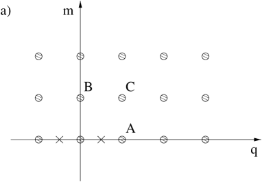
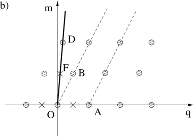
Figure 1: The grids of the electric-magnetic charges in the $SU(2)$ gauge theory. The charges $\{q,m\}$ are measured with respect to the $U(1)$ subgroup of $SU(2)$, as in Sect. 1.5. The closed circles indicate the charges in the theory with the adjoint ($SU(2)$ triplet) matter. The crosses indicate the electric charge of the matter field in the fundamental ($SU(2)$ doublet) representation. ($a$) The rectangular grid corresponding to $\vartheta=0$. The point denoted by $C$ is a bound state of the triplet matter quantum with the monopole. Bound states of the doublet matter quanta with monopoles are possible too (but not indicated). ($b$) The oblique grid corresponding to $\vartheta=\pi+\varepsilon$, $0<\varepsilon\ll\pi$. The state denoted by $D$ is a dyon with a small value of the electric charge, which presumably condenses. The point denoted by $F$ is an unconfined bound state of the quark and dyon $B$. Its external quantum numbers are those of the quark.

The magnetic monopole lies on the vertical axis (point $B$). It has $m=1,\,\,q=0$. Other states on the vertical axis are anti-monopole, a pair of monopoles and so on. All points which do not belong to the horizontal and vertical axis are bound states of electric and magnetic quanta. Note that the monopole condensation automatically precludes from condensation all states carrying the electric charge, since their mass squared is positive (and infinite). The latter are confined. All states which do not lie on the straight line connecting the origin with the point $B$ are confined by the flux tubes of the chromoelectric field attached to them.

Increasing $\vartheta$ we deform the $\{q,m\}$ grid in a continuous way. When $\vartheta$ is close to $\pi$, but slightly larger than $\pi$, we arrive at the grid shown on Fig. 1$b$. It is quite obvious that if $\vartheta\neq 0$ or $2\pi$ the grid of all possible values of $\{q,m\}$ is oblique. (That’s where the name oblique confinement comes from.) At $\vartheta=\pi$ the objects with $m=1$ will have $q=\pm 1/2,\pm 3/2$ and so on. It may well happen that the $m=1$ objects will not condense, since apart from the magnetic charge they have large (and opposite) electric charges. But among the $m=2$ monopoles there is one with the vanishing electric charge, and it is quite conceivable that energetically it is more expedient for these objects to condense. If $\vartheta$ is slightly larger than $\pi$ the state suspect of condensing is that marked by $D$ on Fig. 1$b$. All states that do not lie on the straight line connecting the origin with $D$ will be confined. This is a very peculiar confinement, however. Some of the states, carrying the external quantum numbers of the fundamental quarks, exist in the observable spectrum. The quarks themselves (crosses on the horizontal axis) do not lie on the $OD$ line and, hence, are confined. The bound state of the quark and a dyon (the cross marked by the letter $F$) does belong to this line, and is not confined. Since the dyon has no baryon charge, or any other external quantum number, the state $E$ has exactly the same baryon charge as the fundamental quark, i.e. it is a fractional.

One has to pay a price for having fractionals in the observable spectrum. As explained in [3], even though the quarks are described by the Fermi fields at the Lagrangian level, the states with the fractional (and non-vanishing) baryon charge to be observed will all be bosons!

1.5 QCD monopoles and Abelian projection

Let us discuss how monopole-like configurations could emerge in QCD. Following ’t Hooft we will impose an incomplete gauge fixing condition in a special way. In the Georgi-Glashow model the Higgs mechanism breaks the original $SU(2)$ down to $U(1)$, which paves the way to the emergence of the monopoles as physical objects. In QCD the gauge group remains unbroken, of course. Our task is to single out an $U(1)$ subgroup by imposing an appropriate gauge condition. The monopole-like solution, obtained in this way certainly cannot be interpreted as a physical particle; it should be viewed rather as a first stage in a construction which, eventually, may answer the question whether the dual Meissner effect takes place in QCD.

That the monopole-like solutions of the classical equations of motion are present in QCD can be seen in many different ways. For instance, assume that (an incomplete) gauge condition is imposed in such a way that the time-dependent gauge transformations are forbidden. Whatever this gauge condition might be it still does not forbid the gauge transformations which depend on the spatial coordinates, $\vec{x}$. For simplicity we will additionally assume that the gauge group is $SU(2)$, not $SU(3)$ as in genuine QCD. Under this narrow class of gauge transformations $A_{0}^{a}A_{0}^{a}$ is obviously gauge invariant, since with respect to the spatial-dependent gauge transformations the time component of $A$ transforms homogeneously. If so, the model becomes identical to the BPS limit of the Georgi-Glashow model in the $A_{0}=0$ gauge, which is known to possess the monopole solutions.

Let us elucidate the latter assertion in more detail. The Lagrangian of the $SU(2)$ Yang-Mills theory in the above “gauge”, for the static field configurations, takes the form

$${\cal L}=-\frac{1}{4}G_{ij}^{a}(\vec{x})G_{ij}^{a}(\vec{x})+\frac{1}{2}D_{i}A_{0}^{a}(\vec{x})D_{i}A_{0}^{a}(\vec{x})\,,$$ (1.26)

where

$$D_{i}A_{0}^{a}=\partial_{i}A_{0}+g\epsilon^{abc}A_{i}^{b}A_{0}^{c}$$

is the covariant derivative. If we now rename $A_{0}^{a}\rightarrow i\phi^{a}$, the Lagrangian (1.26) will coincide with that of the Georgi-Glashow model in the $A_{0}=0$ gauge (in the BPS limit) . The classical equations of motion are identical and should then have identical solutions; in particular, the monopole solution (1.14) goes through. In the case at hand $v^{2}$ is the value of $A_{0}^{a}A_{0}^{a}$ at the spatial infinity. Since the time-dependent gauge transformation are forbidden, this value is well-defined.

I pause here to make a few explanatory remarks. The ’t Hooft-Polyakov monopole in the BPS limit satisfies the condition (1.11). One immediately recognizes in this condition in our particular case the self-duality equation $G_{\mu\nu}=(1/2)\epsilon_{\mu\nu\alpha\beta}G_{\alpha\beta}$ defining the (multi)instanton solutions. Thus, heuristically it is clear that the “monopole” solution we have found must be equivalent (up to a gauge transformation) to a chain of instantons. Since the “monopole” mass is finite, the action is infinite; therefore, we deal here with an infinite chain of instantons. The fact that the equivalence does indeed take place was demonstrated in Ref. [21] where it was established that the monopole can be identified with a sequence of equally spaced instantons located at the time axis. The spacing between the instanton centers is $8\pi^{2}M_{\rm mon}^{-1}g^{-2}$, and their radii tend to infinity. Some other chains were shown to be gauge-equivalent to dyons [22]. The inverse transition, from instantons to monopoles, was also studied. It was found that the instanton considered in the Abelian projection (see below) coincides with a closed monopole loop centered at the instanton center [23]. For a discussion of the transition from the “monopoles” to the instanton chains and back see Ref. [24].

Those readers who feel uneasy with the notion of monopoles in QCD can think of the solution above as of a sequence of instantons. The instantons are, of course, much more familiar to the QCD practitioners.

A related but somewhat more general line of reasoning leading to the same monopole-like configurations was suggested by ’t Hooft [3]. His Abelian projection of QCD can be elucidated as follows. Let us consider some gauge non-invariant operator in the adjoint representation of the gauge group transforming homogeneously. In pure gluodynamics this may be, say, $G_{12}^{a}$. If quarks are present one might consider $\bar{\psi}_{i}\psi^{j}$ where $i$ and $j$ are color indices. It may be more convenient, however, to introduce (auxiliary) scalar fields in the adjoint representation, $\phi^{a}$, making them sufficiently heavy, so they do not affect the low-energy physics. Generically, this operator will be denoted as $X_{i}^{j}\equiv X^{a}(T^{a})_{i}^{j}$ where the matrices $T^{a}$ are the generators of the gauge group. For simplicity we will assume that the gauge group is $SU(N)$; then, $(T^{a})_{i}^{j}$ are $N$ by $N$ matrices generalizing the Gell-Mann matrices of QCD. The gauge transformation acts on $X$ as $X\rightarrow UXU^{-1}$ where $U$ is arbitrary $x$ dependent matrix from $SU(N)$. It is quite obvious that by choosing $U(x)$ in an appropriate way it is always possible to diagonalize $X$. In other words, the only components of $X^{a}$ surviving after the gauge transformation are those corresponding to the Cartan subalgebra of $SU(N)$: $a=3,8,15$ and so on. This “Abelization” of the operator $X$ obviously explains why the gauge is referred to as the Abelian projection.

The gauge condition above is an incomplete gauge, since one can additionally perform gauge transformations corresponding to arbitrary rotations around the third, eighth and so on axis without destroying the Abelian nature of $X$. The diagonal form of the matrix $X$ is preserved under these rotations: all generators $T^{3}$, $T^{8}$, $T^{15}$, … are diagonal. Thus, in the gauge at hand, $U(1)^{N-1}$ subgroup is singled out, $SU(N)$ gluodynamics looks similar to QED, with $N-1$ different photons ($A^{3},A^{8},A^{15}$, etc.) and $(1/2)N(N-1)$ “matter fields” (all off-diagonal $A$’s) charged with respect to the photon fields. The values of the charges are, generally speaking, different for different photons. They depend on the group constants.

Intuitively it is clear that we are going to have the “monopole” solutions. Formally, this can be seen as follows. In the Abelian projection the operator $X$ is a diagonal matrix, $X=$ diag$\{\lambda_{1},\lambda_{2},...,\lambda_{N}\}$ where the eigenvalues $\lambda$ may be ordered, $\lambda_{1}>\lambda_{2}>...>\lambda_{N}$. In some exceptional points in space, however, two out of $N$ eigenvalues can coincide, say $\lambda_{1}$ and $\lambda_{2}$. This singles out the upper left $SU(2)$ corner of $SU(N)$ with a monopole sitting at the point where $\lambda_{1}=\lambda_{2}$.

Indeed, close to this point we can focus on the upper left two-by-two corner of the matrix $X$, assuming that the remaining part of the matrix is already diagonal, with non-coinciding eigenvalues. We have to diagonalize only the upper left corner. Near the point ${\vec{x}}_{0}$ where $\lambda_{1}=\lambda_{2}$ the two-by-two submatrix has the form

$$\lambda{\bf 1}+\varepsilon^{a}(\vec{x})\sigma^{a}$$

where 1 is the two-by-two unit matrix and $\sigma^{a}$ are the Pauli matrices. The condition $\lambda_{1}=\lambda_{2}$ at ${\vec{x}}_{0}$ means that $\varepsilon^{a}=0$ at $\vec{x}={\vec{x}}_{0}$ ($a=1,2,3$). Since we have to ensure that three (real) functions vanish, generically this can happen only on manifold of dimension zero, i.e. in isolated points in space, as was mentioned. Moreover, near these points $\varepsilon^{a}(\vec{x})$ has a hedgehog configuration, $\varepsilon^{a}(\vec{x})\sim(x-{x}_{0})^{a}$, a characteristic feature of the ’t Hooft-Polyakov monopole.

In the absence of a genuinely small parameter in QCD, the semi-classical description sketched above cannot lead us too far beyond a qualitative picture. Definitely, there is no way one can study the monopole condensation, a crucial element of the confinement mechanism-to-be, in this approximation. One can try, however, to apply these ideas in the context of the lattice simulations, hoping to get precious insights from numerical studies. Although work in this direction is far from completion, and many aspects remain unclear (see e.g. Ref. [25]), some initial results are quite encouraging. In particular, the abundance of the monopoles in the vacuum ensemble of the lattice QCD was observed, and a connection with the chiral symmetry breaking conjectured [26]. Approaches combining analytical methods with numerical analysis are under investigation (see e.g. [27]).

Summarizing, we have learned that the gauge theories can be in the following phases:

1) Coulomb (Abelian and non-Abelian; in the latter case the infrared limit is conformal, as will be discussed in detail in Sect. 3);

2) free (Landau);

3) Higgs (a possible version is a unified Higgs/confining phase);

4) confining (a possible version is oblique confinement).

Now that we are familiar with various dynamical scenarios one expects to observe in different gauge theories, we are ready to proceed to supersymmetric theories where, in some cases, it is possible to go far beyond qualitative ideas, towards exact solution, using miracles of supersymmetry.

2 Lecture 2. Basics of Supersymmetric Gauge Theories

The dream of every QCD practitioner is to find analytic solutions of two most salient properties of QCD: color confinement and spontaneous breaking of the chiral symmetry. In spite of two decades of vigorous efforts very little progress is made in this direction. At the same time, exciting developments took place, mostly in the last few years, in supersymmetric gauge theories – close relatives of QCD. These developments can, eventually, lead to a breakthrough in QCD. Even if this does not happen, they are very interesting on their own. It turns out that supersymmetry helps reveal several intriguing and extremely elegant properties which shed light on subtle aspects of the gauge theories in general. In this section we will start our excursion in supersymmetric gauge theories. There is a long way to go, however, before we will be able to discuss a variety of fascinating results obtained in this field recently. As a first step let me briefly review some basic elements of the formalism we will need below.

2.1 Introducing supersymmetry

Supersymmetry relates bosonic and fermionic degrees of freedom. A necessary condition for any theory to be supersymmetric is the balance between the number of the bosonic and fermionic degrees of freedom, having the same mass and the same “external” quantum numbers, e.g. color. Let us consider several simplest examples of practical importance.

A scalar complex field $\phi$ has two degrees of freedom (a particle plus antiparticle). Correspondingly, its spinor superpartner is the Weyl (two-component) spinor, which also has two degrees of freedom – say, the left-handed particle and the right-handed antiparticle. Alternatively, instead of working with the complex fields, one can introduce real fields, with the same physical content: two real scalar fields $\phi_{1}$ and $\phi_{2}$ describing two “neutral” spin-0 particles, plus the Majorana (real four-component) spinor describing a “neutral” spin-1/2 particle with two polarizations. (By neutral I mean that the corresponding antiparticles are identical to their particles). This family has a balanced number of the degrees of freedom both in the massless and massive cases. Below we will see that in the superfield formalism it is described, in a concise form, by one chiral superfield.

When we speak of the quark flavors in QCD we count the Dirac spinors. Each Dirac spinor is equivalent to two Weyl spinors. Therefore, in SQCD each flavor requires two chiral superfields. Sometimes, the superfields from this chiral pair are referred to as subflavors. Two subflavors comprise one flavor.

Another important example is vector particles, gauge bosons (gluons in QCD, $W$ bosons in the Higgs phase). Each gauge boson carries two physical degrees of freedom (two transverse polarizations). The appropriate superpartner is the Majorana spinor. Unlike the previous example the balance is achieved only for massless particles, since the massive vector boson has three, not two, physical degrees of freedom. The superpartner to the massless gauge boson is called gaugino. Notice that the mass still can be introduced through the (super)Higgs mechanism. We will discuss the Higgs mechanism in supersymmetric gauge theories later on.

In counting the degrees of freedom above the external quantum numbers were left aside. Certainly, they should be the same for each member of the superfamily. For instance, if the gauge group is SU(2), the gauge bosons are “color” triplets, and so are gauginos. In other words, the Majorana fields describing gauginos are provided by the “color” index $a$ taking three different values, $a=1,2,3$.

If we consider the free field theory with the balanced number of degrees of freedom, the vacuum energy vanishes. Indeed, the vacuum energy is the sum of the zero-point oscillation frequencies for each mode of the theory,

$$E_{\rm vac}=\sum_{\vec{k}}\left\{\omega^{\rm boson}_{\vec{k}}-\omega^{\rm ferm}_{\vec{k}}\right\}\,.$$ (2.1)

I remind that the modes are labeled by the three-momentum $\vec{k}$; say, for massive particles

$$\omega_{\vec{k}}=\sqrt{m^{2}+{\vec{k}}^{2}}\,.$$

It is important that the boson and fermion terms enter with the opposite signs and cancel each other, term by term. This observation, which can be considered as a precursor to supersymmetry, was made by Pauli in 1950 [28]! If interactions are introduced in such a way that supersymmetry remains unbroken, the vanishing of the vacuum energy is preserved in dynamically nontrivial theories.

Balancing the number of degrees of freedom is the necessary but not sufficient condition for supersymmetry in dynamically nontrivial theories, of course. All vertices must be supersymmetric too. This means that each line can be substituted by that of a superpartner. Let us consider, for instance, QED, the simplest gauge theory. We start from the electron-electron-photon coupling (Fig. 2$a$). Now, as we already know, in SQED the electron is accompanied by two selectrons (two, because the electron is described by the four-component Dirac spinor rather than the Weyl spinor). Thus, supersymmetry requires the selectron-selectron-photon vertices, (Fig. 2$b$), with the same coupling constant. Moreover, the photon can be substituted by its superpartner, photino, which generates the electron-selectron-photino vertex (Fig. 2$c$), with the same coupling. In the old-fashioned language of the pre-SUSY era we would call this vertex the Yukawa coupling. In the supersymmetric language this is the gauge interaction since it generalizes the gauge interaction coupling of the photon to the electron.

Figure 2: Interaction vertices in QED and its supergeneralization, SQED. ($a$) $\bar{e}e\gamma$ vertex; ($b$) selectron coupling to photon; ($c$) electron-selectron-photino vertex. All vertices have the same coupling constant. The quartic self-interaction of selectrons is also present, but not shown.

With the above set of vertices one can show that the theory is supersymmetric at the level of trilinear interactions, provided that the electrons and the selectrons are degenerate in mass, while the photon and photino fields are both massless. To make it fully supersymmetric one should also add some quartic terms, describing self-interactions of the selectron fields, as we will see shortly.

Now, the theory is dynamically nontrivial, the particles – bosons and fermions – are not free and still $E_{vac}=0$. This is the first miracle of supersymmetry.

The above pedestrian (or step-by-step) approach to supersymmetrizing the gauge theories is quite possible, in principle. Moreover, historically the first supersymmetric model derived by Golfand and Likhtman, SQED, was obtained in this way [4]. This is a painfully slow method, however, which is totally out of use at the present stage of the theoretical development. The modern efficient approach is based on the superfield formalism, introduced in 1974 by Salam and Strathdee [29] who replaced the conventional four-dimensional space by the superspace.

2.2 Superfield formalism: bird’s eye view

I will be unable to explain this formalism, even briefly. The reader is referred to the text-books and numerous excellent reviews, see the list of recommended literature at the end. Below some elements are listed mostly with the purpose of introducing relevant notations, to be used throughout the entire lecture course. (Our notation, conventions and useful formulae are collected in Appendix.)

If the conventional space-time is parametrized by the coordinate four-vector $x_{\mu}$, the superspace is parametrized by $x_{\mu}$ and two Grassmann variables, $\theta$ and $\bar{\theta}$. The Grassmann numbers obey all standard rules of arithmetic except that they anticommute rather than commute with each other. In particular, the product of a Grassmann number with itself is zero, for this reason.

With respect to the Lorentz properties, $\theta$ and $\bar{\theta}$ are spinors. As well known, the four-dimensional Lorenz group is equivalent to $SU(2)\times SU(2)$ and, therefore, there exist two types of spinors, left-handed and right-handed, denoted by undotted and dotted indices, respectively; $\theta_{\alpha}$ is the left-handed spinor while $\bar{\theta}_{\dot{\alpha}}$ is the right-handed one ($\alpha,\dot{\alpha}=1,2$). The indices of the right-handed spinors are supplied by dots to emphasize the fact that their transformation law does not coincide with that of the left-handed spinors.

The Lorentz scalars can be formed as a convolution of two dotted or two undotted spinors, $\theta^{\alpha}\theta_{\alpha}$ or $\bar{\theta}_{\dot{\alpha}}\bar{\theta}^{\dot{\alpha}}$, with one lower and one upper index. Raising and lowering of indices is realized by virtue of the antisymmetric (Levi-Civita) symbol,

$$\bar{\theta}_{\dot{\alpha}}=\epsilon_{\dot{\alpha}\dot{\beta}}\bar{\theta}^{\dot{\beta}}\,,\,\,\,\,\theta_{\alpha}=\epsilon_{\alpha\beta}\theta^{\beta}\,,$$

where

$$\epsilon^{12}=\epsilon^{\dot{1}\dot{2}}=1\,;\,\,\,\,\epsilon_{12}=\epsilon_{\dot{1}\dot{2}}=-1$$

so that $\epsilon^{\alpha\beta}\epsilon_{\beta\gamma}=\delta^{\alpha}_{\gamma}$. When one raises or lowers the index of $\theta$ the $\epsilon$ symbol must be placed to the left of $\theta$.

A shorthand notation when the indices of the spinors are implicit is widely used, for instance,

$$\theta^{2}\equiv\theta^{\alpha}\theta_{\alpha}$$

and

$$\bar{\theta}^{2}\equiv\bar{\theta}_{\dot{\alpha}}\theta^{\dot{\alpha}}\,.$$

Notice that in convoluting the undotted indices one writes first the spinor with the upper index while for the dotted indices the first spinor has the lower index. The ordering is important since the elements of the spinors are anticommuting Grassmann numbers.

It remains to be added that the vector quantities can be obtained from two spinors – one dotted and one undotted. Thus, $\theta_{\alpha}\bar{\theta}_{\dot{\alpha}}$ transforms as a Lorentz vector.

Now, we can introduce the notion of supertranslations in the superspace $\{x,\theta,\bar{\theta}\}$. The generic supertransformation has the form

$$\theta\rightarrow\theta+\varepsilon\,,\,\,\,\,\bar{\theta}\rightarrow\bar{\theta}+\bar{\varepsilon}\,,$$

$$x_{\alpha\dot{\beta}}\rightarrow x_{\alpha\dot{\beta}}+2i\varepsilon_{\alpha}\bar{\theta}_{\dot{\beta}}-2i\theta_{\alpha}\bar{\varepsilon}_{\dot{\beta}}\,.$$ (2.2)

The supertranslations generalize conventional translations in the ordinary space.

One can also consider the so called chiral and antichiral superspaces (chiral realizations of the supergroup); the first one does not explicitly contain $\bar{\theta}$ while the second does not contain $\theta$. It is not difficult to see that a point from the chiral superspace is parametrized by $\{x_{L},\theta\}$, and that from the antichiral superspace is parametrized by $\{x_{R},\bar{\theta}\}$. Here

$$(x_{L})_{\alpha\dot{\alpha}}=x_{\alpha\dot{\alpha}}-2i\theta_{\alpha}\bar{\theta}_{\dot{\alpha}}\,,\,\,\,(x_{R})_{\alpha\dot{\alpha}}=x_{\alpha\dot{\alpha}}+2i\theta_{\alpha}\bar{\theta}_{\dot{\alpha}}\,.$$ (2.3)

Under this definition the supertransformations corresponding to the shifts in $\theta$ and $\bar{\theta}$, respectively, leave us inside the corresponding superspace. Indeed, if $\theta\rightarrow\theta+\varepsilon$ and $\bar{\theta}\rightarrow\bar{\theta}+\bar{\varepsilon}$, then

$$(x_{L})_{\alpha\dot{\beta}}\rightarrow(x_{L})_{\alpha\dot{\beta}}-4i\theta_{\alpha}\bar{\varepsilon}_{\dot{\beta}}\,\,\,\mbox{and}\,\,\,(x_{R})_{\alpha\dot{\beta}}\rightarrow(x_{R})_{\alpha\dot{\beta}}+4i\varepsilon_{\alpha}\bar{\theta}_{\dot{\beta}}\,.$$ (2.4)

Superfields provide a very concise description of supersymmetry representations. They are very natural generalizations of conventional fields. Say, the scalar field $\phi(x)$ in the $\lambda\phi^{4}$ theory is a function of $x$. Correspondingly, superfields are functions of $x$ and $\theta$’s. For instance, the chiral superfield $\Phi(x_{L},\theta)$ depends on $\theta$ and $x_{L}$ (and has no explicit $\bar{\theta}$ dependence). If we Taylor-expand it in the powers of $\theta$ we get the following formula:

$$\Phi(x_{L},\theta)=\phi(x_{L})+\sqrt{2}\psi(x_{L})\theta+\theta^{2}F(x)\,.$$ (2.5)

There are no higher-order terms in the expansion since higher powers of $\theta$ vanish due to the Grassmannian nature of this parameter. For the same reason the argument of the last component of the chiral superfield, $F$, is set equal to $x$. The distinction between $x$ and $x_{L}$ is not important in this term. The last component of the chiral superfield is always called $F$. $F$ terms of the chiral superfields are non-dynamical, they appear in the Lagrangian without derivatives. We will see later that $F$ terms play a distinguished role.

The lowest component of the chiral superfield is a complex scalar field $\phi$, and the middle component is a Weyl spinor $\psi$. Each of these fields describes two degrees of freedom, so the appropriate balance is achieved automatically. Thus, we see that superfield is a concise form of representing a set of components. The transformation law of the components follows immediately from Eq. (2.4), for instance, $\delta\phi(x)=\sqrt{2}\psi(x)\varepsilon$, and so on.

The antichiral superfields depend on $x_{R}$ and $\bar{\theta}$. The chiral and antichiral superfields describe the matter sectors of the theories to be studied below. The gauge field appears from the so called vector superfield $V$ which depends on both, $\theta$ and $\bar{\theta}$ and satisfies the condition $V=V^{\dagger}$. The component expansion of the vector superfield has the form

$$V(x,\theta,\bar{\theta})=C(x)+i\theta\chi(x)-i\bar{\theta}\bar{\chi}(x)+\frac{i}{2}\theta^{2}[M(x)+iN(x)]-\frac{i}{2}\bar{\theta}^{2}[M(x)-iN(x)]-$$

$$2\theta_{\alpha}\bar{\theta}_{\dot{\beta}}v^{\alpha\dot{\beta}}(x)+2\left\{i\theta^{2}\bar{\theta}_{\dot{\beta}}\left[\bar{\lambda}^{\dot{\beta}}-\frac{i}{4}\partial^{\alpha\dot{\beta}}\chi_{\alpha}\right]+\mbox{h.c.}\right\}+\theta^{2}\bar{\theta}^{2}\left[D(x)-\frac{1}{4}\Box C(x)\right]\,.$$ (2.6)

The components $C,D,M,N$ and $v^{\alpha\dot{\beta}}$ must be real to satisfy the condition $V=V^{\dagger}$. The vector field $v^{\alpha\dot{\beta}}$ gives its name to the entire superfield.

The last component of the vector superfield, apart from a full derivative, is called the “ $D$ term”. $D$ terms also play a special role.

Let me say a few words about the gauge transformations. For simplicity I will consider the case of the Abelian (U(1)) gauge group. In the non-Abelian case the corresponding formulae become more bulky, but the essence stays the same.

As well known , in nonsupersymmetric gauge theories the matter fields transform under the gauge transformations as

$$\phi(x)\rightarrow e^{i\alpha(x)}\phi(x)\,,\,\,\,\phi(x)^{\dagger}\rightarrow e^{-i\alpha(x)}\phi(x)^{\dagger}\,,$$ (2.7)

while the gauge field

$$v_{\mu}(x)\rightarrow v_{\mu}(x)+\partial_{\mu}\alpha(x)\,,$$ (2.8)

where $\alpha(x)$ is an arbitrary function of $x$. Equations (2.7) and (2.8) prompt the supersymmetric version of the gauge transformations,

$$\Phi(x_{L},\theta)\rightarrow e^{i\Lambda}\Phi(x_{L},\theta)\,,\,\,\,\bar{\Phi}(x_{R},\bar{\theta})\rightarrow e^{-i\bar{\Lambda}}\Phi(x_{R},\bar{\theta})\,$$ (2.9)

and

$$V\rightarrow V-i(\Lambda-\bar{\Lambda})$$ (2.10)

where $\Lambda$ is an arbitrary chiral superfield, $\bar{\Lambda}$ is its antichiral partner. $\bar{\Phi}e^{V}\Phi$ is then a gauge invariant combination playing the same role as ${\cal D}_{\mu}\phi^{\dagger}{\cal D}_{\mu}\phi$ in non-supersymmetric theories. Let me parenthetically note that supersymmetrization of the gauge transformations, Eqs. (2.9), (2.10), was the path which led Wess and Zumino [30] to the discovery of the supersymmetric theories (independently of Golfand and Likhtman).

In components

$$C\rightarrow C-i(\phi-\phi^{\dagger})\,,\,\,\,\chi\rightarrow\chi-\sqrt{2}\psi\,,\,\,\,M+iN\rightarrow M+iN-2F\,$$

$$v_{\alpha\dot{\beta}}\rightarrow v_{\alpha\dot{\beta}}+\partial_{\alpha\dot{\beta}}(\phi+\phi^{\dagger})\,,\,\,\,\lambda\rightarrow\lambda\,,\,\,\,D\rightarrow D\,.$$ (2.11)

We see that the $C,\chi,M$ and $N$ components of the vector superfield can be gauged away. This is what is routinely done when the component formalism is used. This gauge bears the name of its inventors – it is called the Wess-Zumino gauge. Imposing the Wess-Zumino gauge condition in supersymmetric theory one actually does not fix the gauge completely. The component Lagrangian one arrives at in the Wess-Zumino gauge still possesses the gauge freedom with respect to non-supersymmetric (old-fashioned) gauge transformations.

It remains to introduce spinorial derivatives. They will be denoted by capital $D$ and $\bar{D}$,

$$D_{\alpha}=\frac{\partial}{\partial\theta^{\alpha}}-i\partial_{\alpha\dot{\beta}}\bar{\theta}^{\dot{\beta}}\,,\,\,\,\bar{D}_{\dot{\alpha}}=-\frac{\partial}{\partial\bar{\theta}^{\dot{\alpha}}}+i\partial_{\beta\dot{\alpha}}\theta^{\beta}\,.$$ (2.12)

The relative signs in Eq. (2.12) are fixed by the requirements $D_{\alpha}(x_{R})_{\beta\dot{\gamma}}=0$ and $\bar{D}_{\dot{\alpha}}(x_{L})_{\beta\dot{\gamma}}=0$.

To make the spinorial derivatives distinct from the regular covariant derivative the latter will be denoted by the script ${\cal D}$. The supergeneralization of the field strength tensor of the gauge field has the form

$$W_{\alpha}(x_{L},\theta)=\frac{1}{8}\bar{D}^{2}(e^{-V}D_{\alpha}e^{V})=$$

$$i\lambda_{\alpha}(x_{L})-\theta_{\alpha}D(x_{L})-i\theta^{\beta}G_{\alpha\beta}(x_{L})+\theta^{2}{\cal D}_{\alpha\dot{\alpha}}\bar{\lambda}^{\dot{\alpha}}(x_{L})\,,$$ (2.13)

where $G_{\alpha\beta}$ is the gauge field strength tensor in the spinorial form.

This brief excursion in the formalism, however boring it might seem, is necessary for understanding physical results to be discussed below. I will try to limit such excursions to absolute minimum, but we will not be able to avoid them completely. Now, the stage is set, and we are ready to submerge in the intricacies of the supersymmetric gauge dynamics.

2.3 Simplest supersymmetric models

In this section we will discuss some simple models. Our basic task is to reveal general features playing the key role in various unusual dynamical scenarios realized in supersymmetric gauge theories. One should keep in mind that all theories with matter can be divided in two distinct classes: chiral and non-chiral matter. The second class includes supersymmetric generalization of QCD, and all other models where each matter multiplet is accompanied by the corresponding conjugate representation. In other words, mass term is possible for all matter fields. Even if the massless limit is considered, the very possibility of adding the mass term is very important for dynamics. In particular, dynamical SUSY breaking cannot happen in the non-chiral models.

Models with chiral matter are those where the mass term is impossible. The matter sector in such models is severely constrained by the absence of the internal anomalies in the theory. The most well-known example of this type is the $SU(5)$ model with equal number of chiral quintets and (anti)decuplets. Each quintet and anti-decuplet, together, are called generation; when the number of generations is three this is nothing but the most popular grand unified theory of electroweak interactions. The chiral models are singled out by the fact that dynamical SUSY breaking is possible, in principle, only in this class. In the present lecture course dynamical SUSY breaking is not our prime concern. Rather, we will focus on various non-trivial dynamical regimes. Most of the regimes to be discussed below manifest themselves in the non-chiral models, which are simpler. Therefore, the emphasis will be put on the non-chiral models, digression to the chiral models will be made occasionally.

2.3.1 Supersymmetric gluodynamics

To begin with we will consider supersymmetric generalization of pure gluodynamics – i.e. the theory of gluons and gluinos. The Lagrangian has the form [31]

$${\cal L}=-\frac{1}{4g^{2}}G_{\mu\nu}^{a}G_{\mu\nu}^{a}+\frac{\vartheta}{32\pi^{2}}G_{\mu\nu}^{a}\tilde{G}_{\mu\nu}^{a}+\frac{i}{2g^{2}}\bar{\lambda}^{a}{\cal D}_{\mu}\gamma^{\mu}\lambda^{a}$$ (2.14)

where $G_{\mu\nu}^{a}$ is the gluon field strength tensor, $\tilde{G}_{\mu\nu}^{a}$ is the dual tensor, $g$ is the gauge coupling constant, $\vartheta$ is the vacuum angle, and ${\cal D}_{\mu}$ is the covariant derivative. Moreover, $\lambda^{a}$ is the gluino field, which can be described either by a four-component Majorana (real) fields or two-component Weyl (complex) fields.

In terms of superfields

$${\cal L}=\frac{1}{4g^{2}_{0}}\,\mbox{Tr}\,\int d^{2}\theta\,W^{2}+\,\mbox{H.c.}\,,$$ (2.15)

where the superfield $W$ is a color matrix,

$$W=W^{a}T^{a}\,,$$

$T^{a}$ are the generators of the gauge group (in the fundamental representation), Tr$T^{a}T^{b}=(1/2)\delta^{ab}$. It is very important that the gauge constant $1/g^{2}_{0}$ in Eq. (2.15) can be treated as a complex parameter. The subscript 0 emphasizes the fact that the gauge couplings in Eqs. (2.15) and (2.14) are different,

$$\frac{1}{g_{0}^{2}}=\frac{1}{g^{2}}-i\frac{\vartheta}{8\pi^{2}}\,,$$ (2.16)

its real part is the conventional gauge coupling while the imaginary part is proportional to the vacuum angle. Thus, the gauge coupling becomes complexified in SUSY theories. This fact has far-reaching consequences.

Equivalence between Eqs. (2.15) and (2.14) is clear from Eq. (2.13). The $F$ component of $W^{2}$ includes the kinetic term of the gaugino field (or gluino, I will use these terms indiscriminately),

$$\bar{\lambda}{\cal D}_{\mu}\gamma^{\mu}\lambda\,,$$

and that of the gauge field,

$$G_{\mu\nu}^{a}G_{\mu\nu}^{a}+iG_{\mu\nu}^{a}\tilde{G}_{\mu\nu}^{a}\,.$$

Superficially the model looks very similar to conventional QCD; the only difference is that the quark fields belonging to the fundamental representation of the gauge group in QCD are replaced by the gluino field belonging to the adjoint representation in supersymmetric gluodynamics. Like QCD, supersymmetric gluodynamics is a strong coupling non-Abelian theory. Therefore, it is usually believed that

$\bullet$ only colorless asymptotic state exist;

$\bullet$ the Wilson loop (in the fundamental representation) is subject to the area law (confinement);

$\bullet$ a mass gap is dynamically generated; all particles in the spectrum are massive.

I would like to stress the word “believe” since the above features are hypothetical. Although the theory does indeed look pretty similar to QCD, supersymmetry brings in remarkable distinctions – some quantities turn out to be exactly calculable. Namely, we know that the gluino condensate develops,

$$\langle\lambda^{a\alpha}\lambda^{a}_{\alpha}\rangle=\mbox{const.}\times\Lambda^{3}e^{2\pi ik/N_{c}}$$ (2.17)

where $N_{c}$ is the number of colors ($SU(N_{c})$ gauge group is assumed and the vacuum angle $\vartheta$ is set equal to zero), $\Lambda$ is the scale parameter of supersymmetric gluodynamics, $k$ is an integer ($k=0,1,...,N_{c}-1$), and the constant in Eq. (2.17) is exactly calculable [32, 33]. A discrete $Z_{2N_{c}}$ symmetry of the model, a remnant of the anomalous $U(1)$, is spontaneously broken by the gluino condensate down to $Z_{2}$. Correspondingly, there are $N_{c}$ degenerate vacua, counted by the integer parameter $k$. Supersymmetry is unbroken – all vacua have the vanishing energy density.

Moreover, the Gell-Mann–Low function of the model, governing the running of the gauge coupling constant, is also exactly calculable [36],

$$\beta(\alpha)=-\frac{3N_{c}\alpha^{2}}{2\pi}\,\frac{1}{1-N_{c}\alpha/(2\pi)}\,.$$ (2.18)

By “exactly” I mean that all orders of perturbation theory are known, and one can additionally show that in the case at hand there are no nonperturbative contributions.

Equations (2.17) and (2.18) historically were the first examples of non-trivial (i.e. non-vanishing) quantities exactly calculated in four-dimensional field theories in the strong coupling regime. These examples, alone, show that the supersymmetric gauge dynamics is full of hidden miracles. We will encounter many more examples in what follows. Eventually, after learning more about supersymmetric theories, you will be able to understand how Eqs. (2.17) and (2.18) are derived. But this will take some time. Here I would like only to add an explanatory remark regarding the vacuum degeneracy in supersymmetric gluodynamics. At the classical level Lagrangian (2.14) has a U(1) symmetry corresponding to the phase rotations of the gluino fields,

$$\lambda\rightarrow e^{i\alpha}\lambda\,.$$ (2.19)

The corresponding current is sometimes called the $R_{0}$ current; it is a superpartner of the energy-momentum tensor and the supercurrent. The $R_{0}$ current exists in any supersymmetric theory. Moreover, in conformally invariant theories – and supersymmetric gluodynamics is conformally invariant at the classical level – it is conserved [37]. In the spinor notation the $R_{0}$ current has the form $J_{\alpha\dot{\alpha}}=\bar{\lambda}_{\dot{\alpha}}\lambda_{\alpha}$, while in the Majorana notation the very same current takes the form $J_{\mu}=\bar{\lambda}\gamma_{\mu}\gamma_{5}\lambda$. (Let me parenthetically note that the vector current of the Majorana gluino identically vanishes. The proof of this fact is left as an exercise.) The conservation of the axial current above is broken by the triangle anomaly,

$$\partial^{\mu}J_{\mu}=\frac{N_{c}}{16\pi^{2}}G_{\mu\nu}^{a}\tilde{G}_{\mu\nu}^{a}\,.$$

So, there is no continuous $U(1)$ symmetry in the model. By the same token, the conformal invariance is ruined by the anomaly in the trace of the energy-momentum tensor. As a matter of fact, the divergence of the $R_{0}$ current and the trace of the energy-momentum tensor can be combined in one superfield [38].

However, a remnant of the would-be symmetry remains, in the form of the discrete phase transformations of the type (2.19) with $\alpha=\pi k/N_{c}$. The gluino condensate further breaks this symmetry to $Z_{2}$ corresponding to $\lambda\rightarrow-\lambda$. The number of the degenerate vacuum states, $N_{c}$, coincides with Witten’s index for the $SU(N_{c})$ theory [39], an invariant which counts the number of the boson zero energy states minus the number of the fermion zero energy states. If Witten’s index is non-vanishing supersymmetry cannot be spontaneously broken, of course.

An interesting aspect, related to the discrete degeneracy of the vacuum states, is the $\vartheta$ dependence. What happens with the vacua if $\vartheta\neq 0$? The question was answered in Ref. [33]. The $\vartheta$ dependence of the gluino condensate is

$$\langle\lambda\lambda\rangle_{\vartheta}=\langle\lambda\lambda\rangle_{\vartheta=0}e^{\frac{i\vartheta}{N_{c}}}\,.$$ (2.20)

This shows that the $N_{c}$ vacua are intertwined as far as the $\vartheta$ evolution is concerned. When $\vartheta$ changes continuously from 0 to $2\pi$ the first vacuum becomes second, the second becomes third, and so on, in a cyclic way.

2.3.2 SU(2) SQCD with one flavor

As the next step on a long road leading us to understanding of supersymmetric gauge dynamics we will consider SUSY generalization of SU(2) QCD with the matter sector consisting of one flavor. This model will serve us as a reference point in all further constructions.

Since the gauge group is SU(2) we have three gluons and three superpartners – gluinos.

As far as the matter sector is concerned, let us remember that one quark flavor in QCD is described by a Dirac field, a doublet with respect to the gauge group. One Dirac field is equivalent to two chiral fields: a left-handed and a right-handed, both transforming according to the fundamental representation of SU(2). Moreover, the right-handed doublet is equivalent to the left-handed anti-doublet, which in turn is equivalent to a doublet. The latter fact is specific to the SU(2) group, whose all representations are (pseudo)real. Thus, the Dirac quark reduces to two left-handed Weyl doublet fields.

Correspondingly, in SQCD each of them will acquire a scalar partner. Thus, the matter sector will be built from two superfields, $S_{1}$ and $S_{2}$. In what follows we will use the notation $S_{f}^{\alpha}$ where $\alpha=1,2$ is the color index, and $f=1,2$ is a “subflavor” index. Two subflavors comprise one flavor. The chiral superfield has the usual form, see Eq. (2.5).

In the superfield language the Lagrangian of the model can be represented in a very concise form

$${\cal L}=\frac{1}{2g^{2}_{0}}\,\mbox{Tr}\,\int d^{2}\theta W^{2}+\frac{1}{4}\int d^{2}\theta d^{2}\bar{\theta}\bar{S}_{f}e^{V}S_{f}+\left(\frac{m_{0}}{4}\int d^{2}\theta S^{\alpha f}S_{\alpha f}+\mbox{ H. c.}\right)\,,$$ (2.21)

where the superfields $V$ and $W_{\alpha}$ are matrices in the color space, for instance, $V\equiv V^{a}\tau^{a}/2$, with $\tau^{a}$ denoting the Pauli matrices. The subscript 0 indicates that the mass parameter and the gauge coupling constant are bare parameters, defined at the ultraviolet cut off. In what follows we will omit this subscript to ease the notation in several instances where it is unimportant.

If we take into account the rules of integration over the Grassmann numbers we immediately see that the integral over $d^{2}\theta$ singles out the $\theta^{2}$ component of the chiral superfields $W^{2}$ and $S^{2}$, i.e. the $F$ terms. Moreover, the integral over $d^{2}\theta d^{2}\bar{\theta}$ singles out the $\theta^{2}\bar{\theta}^{2}$ component of the real superfield $\bar{S}e^{V}S$, i.e. the $D$ term.

Note that the SU(2) model under consideration, with one flavor possesses a global SU(2) (“subflavor”) invariance allowing one to freely rotate the superfields $S_{1}\leftrightarrow S_{2}$. This symmetry holds even in the presence of the mass term, see Eq. (2.21), and is specific for SU(2) gauge group, with its pseudoreal representations. All indices corresponding to the SU(2) groups (gauge, Lorentz and subflavor) can be lowered and raised by means of the $\varepsilon$ symbol, according to the general rules.

The Lagrangian presented in Eq. (2.21) is not generic. Renormalizable models with a richer matter sector usually allow for one more type of $F$ terms, namely

$$\int d^{2}\theta S^{3}\,.$$

These terms are called the Yukawa interactions, since one of the vertices they include corresponds to a coupling of two spinors to a scalar. Strictly speaking, they should be called the super-Yukawa terms, since spinor-spinor-scalar vertices arise also in the (super)gauge parts of the Lagrangian. This jargon is widely spread, however; eventually you will get used to it and learn how to avoid confusion. The combination of the $F$ terms $S^{2}+S^{3}$ is generically referred to as superpotential. The conventional potential of self-interaction of the scalar fields stemming from the given superpotential is referred to as scalar potential.

It is instructive to pass from the superfield notations to components. We will do this exercise now in some detail, putting emphasis on those features which are instrumental in the solutions to be discussed below. Once the experience is accumulated the need in the component notation will subside.

Let us start from $W^{2}$. The corresponding $F$ term was already discussed in Sect. 2.3.1. There is one new important point, however. In Sect. 2.3.1 we omitted the square of the $D$ term present in $W^{2}|_{F}$, see Eq. (2.13),

$$\Delta{\cal L}^{(W)}_{D}=\frac{1}{2g^{2}}D^{a}D^{a}\,.$$ (2.22)

If the matter sector of the theory is empty, this term is unimportant. Indeed, the $D$ field enters with no derivatives, and, hence, can be eliminated from the Lagrangian by virtue of the equations of motion. With no matter fields $D=0$. In the presence of the matter fields, however, eliminating $D$ we get a non-trivial term constructed from the scalar fields, which is of a paramount importance. This point will be discussed later; here let me only note that the sign of $D^{2}$ in the Lagrangian, Eq. (2.22), is unusual, positive.

The next term to be considered is $\int d^{2}\theta d^{2}\bar{\theta}\bar{S}e^{V}S$. Calculation of the $D$ component of $\bar{S}e^{V}S$ is a more time-consuming exercise since we must take into account the fact that $S$ depends on $x_{L}$ while $\bar{S}$ depends on $x_{R}$; the both arguments differ from $x$. Therefore, one has to expand in this difference. The factor $e^{V}$ sandwiched between $\bar{S}$ and $S$ covariantizes all derivatives. Needless to say that the field $V$ is treated in the Wess-Zumino gauge. It is not difficult to check that

$$\frac{1}{4}\int d^{2}\theta d^{2}\bar{\theta}\bar{S}_{f}e^{V}S_{f}=\bar{\psi}_{f}i\not\!\!{\cal D}\psi_{f}-\phi^{\dagger}_{f}{\cal D}^{2}\phi_{f}+$$

$$\left[(\psi_{f}\lambda)\phi_{f}^{\dagger}+\mbox{H.c.}\right]+D^{a}\phi^{\dagger}_{f}T^{a}\phi_{f}$$ (2.23)

where $T^{a}$ are the matrices of the color generators. In the SU(2) theory $T^{a}=\tau^{a}/2$. Now we see why the $D^{2}$ term is so important in the presence of matter; $D^{a}$ does not vanish anymore. Moreover, using the equation of motion we can express $D^{a}$ in terms of the squark fields, generating in this way a quartic self-interaction of the scalar fields,

$$V_{D}=\frac{1}{2g^{2}}D^{a}D^{a}\,,\,\,\,\,D^{a}=-\frac{g^{2}}{2}\left(\phi_{1}^{\dagger}\tau^{a}\phi_{1}+\phi_{2}^{\dagger}\tau^{a}\phi_{2}\right)\,.$$ (2.24)

In the old-fashioned language of the pre-SUSY era one would call the term $(\psi_{f}\lambda)\phi_{f}^{\dagger}$ from Eq. (2.23) the Yukawa interaction. The SUSY practitioner would refer to this term as to the gauge coupling since it is merely a supersymmetric generalization of the quark-quark-gluon coupling. I mention these terms here because later on their analysis will help us establish the form of the conserved $R$ currents.

2.3.3 Vacuum valleys

Let us examine the $D$ potential $V_{D}$ more carefully, neglecting for the time being $F$ terms altogether. As well-known, the energy of any state in any supersymmetric theory is positive-definite. The minimal energy state, the vacuum, has energy exactly at zero. Thus, in determining the classical vacuum we must find all field configurations corresponding to vanishing energy. From Eq. (2.24) it is clear that in the Wess-Zumino gauge the classical space of vacua (sometimes called the moduli space of vacua) is defined by the $D$-flatness condition

$$D^{a}=0\,\,\,\mbox{for all}\,\,a\,.$$ (2.25)

More exactly, Eq. (2.25) is called the Wess-Zumino gauge $D$ flatness condition. Since this gauge is always implied, if not stated to the contrary, we will omit the reference to the Wess-Zumino gauge.

The $D$ potential $V_{D}$ represents a quartic self-interaction of the scalar fields, of a very peculiar form. Typically in the $\phi^{4}$ theory the potential has one – at most several – minima. In other words, the space of the vacuum fields corresponding to minimal energy, is a set of isolated points. The only example with a continuous manifold of points of minimal energy which was well studied previously is the spontaneous breaking of a global continuous symmetry, say, U(1) (Sect. 1). In this case all points belonging to this vacuum manifold are physically equivalent. The $D$ potential (2.24) has a specific structure – the minimal (zero) energy is achieved along entire directions corresponding to the solution of Eq. (2.25). It is instructive to think of the potential as of a mountain ridge; the $D$ flat directions then present the flat bottom of the valleys. Sometimes, for transparency, I will call the $D$ flat directions the vacuum valleys. Their existence was first noted in Ref. [40]. As we will see, different points belonging to the bottom of the valleys are physically inequivalent. This is a remarkable feature of the supersymmetric gauge theories.

In the case of the SU(2) theory with one flavor it is not difficult to find the $D$ flat direction explicitly. Indeed, consider the scalar fields of the form

$$\phi_{1}=v\left(\begin{array}[]{c}1\\ 0\end{array}\right)\,,\,\,\,\phi_{2}=v\left(\begin{array}[]{c}0\\ 1\end{array}\right)\,,$$ (2.26)

where $v$ is an arbitrary complex constant. It is obvious that for any value of $v$ all $D^{a}$’s vanish. $D^{1}$ and $D^{2}$ vanish because $\tau^{1,2}$ are off-diagonal matrices; $D^{3}$ vanishes after summation over two subflavors.

It is quite obvious that if $v\neq 0$ the original gauge symmetry SU(2) is totally spontaneously broken. Indeed, under the condition (2.26) all three gauge bosons acquire masses $\sim gv$. Thus, we deal here with the supersymmetric generalization of the Higgs phenomenon. Needless to say that supersymmetry is not broken. It is instructive to trace the reshuffling of the degrees of freedom before and after the Higgs phenomenon. In the unbroken phase, corresponding to $v=0$, we have three massless gauge bosons (6 degrees of freedom), three massless gaugino (6 degrees of freedom), four matter fermions (the Weyl fermions, 8 degrees of freedom), and four matter scalars (complex scalars, 8 degrees of freedom). In the broken phase three matter fermions combine with the gauginos to form three massive Dirac fermions (12 degrees of freedom). Moreover, three matter scalars combine with the gauge fields to form three massive vector fields (9 degrees of freedom) plus three massive (real) scalars. What remains massless? One complex scalar field, corresponding to the motion along the bottom of the valley, $v$, and its fermion superpartner, one Weyl fermion. The balance between the fermion and boson degrees of freedom is explicit.

A gauge invariant description of the system of the vacuum valleys was suggested in Refs. [41, 42] (see also [40]). In these works it was noted that the set of proper coordinates parametrizing the space of the classical vacua is nothing else but the set of all independent (local) products of the chiral matter fields existing in the theory. Since this point is very important let me stress once more that the variables to be included in the set are polynomials built from the fields of one and the same chirality only. These variables are clearly gauge invariant.

At the intuitive level this assertion is almost obvious. Indeed, if there is a $D$ flat direction, the motion along the degenerate bottom of the valley must be described by some effective (i.e. composite) chiral superfield, which is gauge invariant and has no superpotential. The opposite is also true. If we are able to build some chiral gauge invariant (i.e. colorless) superfield $\Phi$, as a local product of the chiral matter superfields of the theory at hand, then the energy is guaranteed to vanish, since (in the absence of the $F$ terms) all terms which might appear in the effective Lagrangian for $\phi$ necessarily contain derivatives. Here $\phi$ is the lowest component of the above superfield $\Phi$. In other words, then, changing the value of $\phi$ we will be moving along the bottom of the valley.

A formal proof of the fact that the classical vacua are fully described by the set of local (gauge invariant) products of the chiral fields comprising the matter sector is given in the recent work [43] which combines and extends results scattered in the literature [40, 41, 44, 45].

The approach based on the chiral polynomials is very convenient for establishing the fact of the existence (non-existence) of the moduli space of the classical vacua, and in counting the dimensionality of this space. For instance, in the SU(2) model with one flavor there exists only one invariant, $S^{2}\equiv S_{\alpha f}S_{\beta g}\epsilon^{\alpha\beta}\epsilon^{fg}=2v^{2}$. Correspondingly, there is only one vacuum valley – one-dimensional complex manifold. The remaining three (out of four) complex scalar fields are eaten up in the super-Higgs phenomenon by the vector fields, which immediately tells us that a generic point from the bottom of the valley corresponds to fully broken gauge symmetry.

In other cases we will have a richer structure of the moduli space of the classical vacua. In some instances no chiral invariants can be built at all. Then the $D$ flat directions are absent.

If the $D$ flat directions exist, and the gauge symmetry is spontaneously broken, then the constraints of the type of Eq. (2.26) can be viewed as a gauge fixing condition. This is nothing else but the unitary gauge in SUSY. Those components of the matter superfields which are set equal to zero are actually eaten up by the vector particles which acquire the longitudinal components through the super-Higgs mechanism.

Although constructing the set of the chiral invariants is helpful in the studies of the general properties of the space of the classical vacua, sometimes it is still necessary to explicitly parametrize the vacuum valleys, just in the same way as it is done in Eq. (2.26). As we have seen, this problem is trivially solvable in the SU(2) model with one flavor. For higher groups and representations the general situation is much more complicated, and the generic solution is not found. Many useful tricks for finding explicit parametrization of the vacuum valleys in particular examples were suggested in Refs. [40, 41, 42]. A few simplest examples are considered below. More complicated instances are considered in the literature. For instance, a parametrization of the valleys in the SU(5) model with two quintets and two antidecuplets was given in Ref. [46] and in the E(6) model with the 27-plet in Ref. [47]. The correspondence between the explicit parametrization of the $D$ flat directions and the chiral polynomials was discussed recently more than once, see e.g. [48] – [52]. I would like to single out Ref. [53] where a catalog of the flat directions in the minimal supersymmetric standard model (MSSM) was obtained by analyzing all possible chiral polynomials and eliminating those of them which are redundant.

Once the existence of the $D$-flat directions is established at the classical level one may be sure that a manifold of the degenerate vacua will survive at the quantum level, provided no $F$ terms appear in the action which might lift the degeneracy. Indeed, in this case the only impact of the quantum corrections is providing an overall $Z$ factor in front of the kinetic term, which certainly does not affect the vanishing of the $D$ terms. The $F$ terms which could lift the degeneracy must be either added in the action by hand (e.g. mass terms), or generated nonperturbatively. A remarkable non-renormalization theorem [54] guarantees that no $F$ terms can be generated perturbatively. We will return to the discussion of this second miracle of SUSY in Sect. 2.4.

In this respect the supersymmetric theories are fundamentally different from the non-supersymmetric ones. Say, in the good old $\phi^{4}$ theory with the Yukawa interaction

$${\cal L}=|\partial_{\mu}\phi|^{2}+\bar{\psi}i\partial_{\mu}\gamma^{\mu}\psi+(g\phi\bar{\psi}\psi+\mbox{H. c.})$$

we could also assume that that the mass and self-interaction of the scalar field vanish at the classical level. Then, classically, we will have a flat direction – any constant value of $\phi$ corresponds to the vanishing vacuum energy. However, this vacuum valley does not survive inclusion of the quantum corrections. Already at the one-loop level both the mass term of the scalar field, and its self-interaction, will be generated, and the continuous vacuum degeneracy will inevitably disappear.

2.3.4 In search of the valleys

Although our excursion in the SU(2) model with one flavor is not yet complete, the issue of the $D$ flat directions is so important in this range of problems that we pause here to do, with pedagogical purposes, a few simple exercises. If you choose to skip this section in the first reading it will be necessary to return to it later.

$SU(N_{c})$ model with $N_{f}$ flavors ($N_{f}<N_{c}$) [41]

The matter sector includes $2N_{f}$ subflavors – $N_{f}$ chiral fields in the fundamental representation of $SU(N_{c})$, $S^{\alpha f}$, and $N_{f}$ chiral fields in the antifundamental representation, $\tilde{S}_{\alpha f}$, where $\alpha=1,...,N_{c}$ and $f=1,...N_{f}$. It is quite obvious that one can form $N_{f}^{2}$ chiral products of the type

$$\tilde{S}_{\alpha}^{f}S^{\alpha g}\,,\,\,\,f,g=1,...,N_{f}\,.$$ (2.27)

All these chiral invariants are independent. Thus, the moduli space of the classical vacua (the vacuum valley) is a complex manifold of dimensionality $N_{f}^{2}$, parametrized by the coordinates (2.27). A generic point from the vacuum valley corresponds to spontaneous breaking of $SU(N_{c})\rightarrow SU(N_{c}-N_{f})$ (except for the case when $N_{f}=N_{c}-1$, when the original gauge group is completely broken). The number of the broken generators is $2N_{c}N_{f}-N_{f}^{2}$; hence, the same amount of the complex scalar fields are eaten up in the super-Higgs mechanism. The original number of the complex scalar fields was $2N_{c}N_{f}$. The remaining $N_{f}^{2}$ degrees of freedom are the moduli (2.27) corresponding to the motion along the bottom of the valley.

In this particular problem it is not difficult to indicate a concrete parametrization of the vacuum field configurations. Indeed, consider a set

$$S_{1}=\tilde{S}_{1}^{\dagger}=v_{1}\left(\begin{array}[]{c}1\\ 0\\ 0\\ ...\\ 0\end{array}\right)\,,S_{2}=\tilde{S}_{2}^{\dagger}=v_{2}\left(\begin{array}[]{c}0\\ 1\\ 0\\ ...\\ 0\end{array}\right)\,,\,\,...\,\,,S_{N_{f}}=\tilde{S}_{N_{f}}^{\dagger}=v_{N_{f}}\left(\begin{array}[]{c}0\\ 0\\ ...\\ 1\\ ...\\ 0\end{array}\right)\,$$ (2.28)

where the unity in $S_{N_{f}}$ occupies the $N_{f}$-th line and $v_{1,2,...,N_{f}}$ are $N_{f}$ arbitrary complex numbers. It is rather obvious that for this particular set all $D$ terms vanish. In verifying this assertion it is convenient to consider first those $D^{a}$’s which lie outside the Cartan subalgebra of $SU(N_{c})$. Since the corresponding $T^{a}$ matrices are off-diagonal each term in the sum $\sum_{f}(S^{\dagger}T^{a}S+\tilde{S}^{\dagger}T^{a}\tilde{S})$ vanishes individually. For the generators from the Cartan subalgebra the fundamentals and anti-fundamentals cancel each other.

The point (2.28) is not a generic point from the bottom of the valley. This is clear from the fact that it is parametrized by only $N_{f}$ complex numbers. To get a generic solution one observes that the theory is invariant under the global $SU(N_{f})\times SU(N_{f})$ flavor rotations (the fundamentals and antifundamentals can be rotated separately). On the other hand, the solution (2.28) is not invariant. Therefore, we can apply a general $SU(N_{f})\times SU(N_{f})$ rotation to Eq. (2.28) without destroying the condition $D^{a}=0$. It is quite obvious that the generators belonging to the Cartan subalgebra of $SU(N_{f})\times SU(N_{f})$ do not introduce new parameters. The remaining rotations introduce $N_{f}^{2}-N_{f}$ complex parameters, to be added to $v_{1}$, …,$v_{N_{f}}$, altogether $N_{f}^{2}$ parameters, as it was anticipated from counting the number of the chiral invariants.

$SU(N_{c})$ model with $N_{f}$ flavors ($N_{f}=N_{c}+1$)

The vacuum valley is parametrized by $N_{f}^{2}$ complex parameters, although the number of the chiral invariants is larger, $N_{f}^{2}+2N_{f}$. Not all chiral invariants are independent. For further details see Sect. 3.1.

$SU(5)$ model with one quintet and one (anti)decuplet

This gauge model describes Grand Unification, with one generation of quarks and leptons. This is our first example of non-chiral matter; it is singled out historically – the instanton-induced dynamical supersymmetry breaking was first found in this model [55]. The quintet field is $V^{\alpha}$, the (anti)decuplet field is antisymmetric $X_{\alpha\beta}$. It is quite obvious that there are no chiral invariants at all. Indeed, the only candidate, $VVX$, vanishes due to antisymmetricity of $X_{\alpha\beta}$. This means that no $D$ flat directions exist. The same conclusion can be reached by explicitly parametrizing $V$ and $X$; inspecting then the $D$-flatness conditions one can conclude that they have no solutions, see e.g. Appendix A in Ref. [56].

$SU(5)$ model with two quintets and two (anti)decuplets and no superpotential

This model (with a small tree-level superpotential term) was the first example of the instanton-induced supersymmetry breaking in the weak coupling regime [57]. It presents another example of the anomaly-free chiral matter sector. Unlike the one-family model (one quintet and one antidecuplet) flat directions do exist (in the absence of superpotential). The system of the vacuum valleys in the two-family $SU(5)$ model was analyzed in Ref. [46]. Generically, the gauge $SU(5)$ symmetry is completely broken, so that 24 out of 30 chiral matter superfields are eaten up in the super-Higgs mechanism. Therefore, the vacuum valley should be parametrized by six complex moduli.

Denote two quintets present in the model as $V_{f}^{\alpha}$ $(f=1,2)$, and two antidecuplets as $(X_{\bar{g}})_{\alpha\beta}$ where ${\bar{g}}=1,2$ and the matrices $X_{\bar{g}}$ are antisymmetric in color indices $\alpha,\beta$. Indices $f$ and ${\bar{g}}$ reflect the $SU(2)_{X}\times SU(2)_{V}$ flavor symmetry of the model. Six independent chiral invariants are

$$M_{\bar{g}}=V_{k}X_{\bar{g}}V_{l}\epsilon^{kl}\,,$$

$$B_{{\bar{g}}f}=X_{\bar{g}}X_{\bar{k}}X_{\bar{l}}V_{f}\epsilon^{{\bar{k}}{\bar{l}}}\,,$$

where the gauge indices in the first line are convoluted in a straightforward manner $V^{\alpha}X_{\alpha\beta}V^{\beta}$, while in the second line one uses the $\epsilon$ symbol,

$$X_{\bar{g}}X_{\bar{k}}X_{\bar{l}}V_{f}=\epsilon^{\alpha\beta\gamma\delta\rho}(X_{\bar{g}})_{\alpha\beta}(X_{\bar{k}})_{\gamma\delta}(X_{\bar{l}})_{\rho\kappa}(V_{f})^{\kappa}\,.$$

The choice of invariants above implies that there are no moduli transforming as $\{4,\,2\}$ under the flavor group (such moduli vanish).

In this model the explicit parametrization of the valley is far from being obvious, to put it mildly. The most convenient strategy of the search is analyzing the five-by-five matrix

$$D^{\alpha}_{\beta}=V^{\alpha}_{f}{\bar{V}}^{f}_{\beta}-2({\bar{X}}^{\bar{g}})^{\alpha\gamma}(X_{\bar{g}})_{\gamma\beta}$$ (2.29)

where ${\bar{V}}=V^{\dagger}$ and ${\bar{X}}=X^{\dagger}$. If this matrix is proportional to the unit one, the vanishing of the $D$ terms is guaranteed. (Similar strategy based on analyzing analogs of Eq. (2.29) is applicable in other cases as well).

A solution of the $D$-flatness condition which contains 7 real parameters looks as follows:

$$V_{1}=\left(\begin{array}[]{c}a_{1}\\ 0\\ 0\\ a_{4}\\ 0\end{array}\right)\,,\,\,\,V_{2}=\left(\begin{array}[]{c}0\\ a_{2}\\ 0\\ 0\\ 0\end{array}\right)\,,$$

$$X_{1}=\frac{1}{\sqrt{2}}\left(\begin{array}[]{ccccc}0&0&0&s&0\\ 0&0&b&0&0\\ 0&-b&0&0&f\\ -s&0&0&0&0\\ 0&0&-f&0&0\end{array}\right)\,,\,\,\,X_{2}=\frac{1}{\sqrt{2}}\left(\begin{array}[]{ccccc}0&d&0&0&g\\ -d&0&0&0&0\\ 0&0&0&0&0\\ 0&0&0&0&h\\ -g&0&0&-h&0\end{array}\right)\,,$$ (2.30)

where

$$|a_{1}|^{2}=r^{2}\cos^{2}\theta\,,\,\,\,|a_{4}|^{2}=r^{2}\cos^{2}\alpha\tan^{2}\theta\,,\,\,\,|a_{2}|^{2}=r^{2}\tan^{2}\theta\frac{\cos^{2}\theta-cos^{2}\alpha}{\sin^{2}\theta+\cos^{2}\alpha}\,,$$

and

$$|s|^{2}=\frac{r^{2}\cos^{2}\alpha}{\cos^{2}\theta{\sin^{2}\theta+\cos^{2}\alpha}}\,,\,\,|b|^{2}=r^{2}{\sin^{2}\theta+\cos^{2}\alpha}\,,\,\,|f|^{2}=r^{2}\frac{\cos^{2}\alpha}{\cos^{2}\theta}{\frac{\cos^{2}\theta-cos^{2}\alpha}{\sin^{2}\theta+\cos^{2}\alpha}}\,,$$

$$|d|^{2}=\frac{r^{2}}{\cos^{2}\theta}{(cos^{2}\theta-cos^{2}\alpha)}\,,\,\,\,|g|^{2}=r\cos^{2}\alpha\,,\,\,\,|h|^{2}=r^{2}\sin^{2}\theta\,.$$ (2.31)

Thus, the absolute values of matrix elements are parametrized by three real parameters $r$, $\alpha$ and $\theta$. Additional 4 parameters appear via phases $\delta$ of 9 elements $a_{i}$, $s$, $b$, $f$, $d$, $g$, $h$. Three phases, out of nine, are related to gauge rotations and are not observable in the gauge singlet sector. Additionally, there are two constraints,

$$\delta_{1}-\delta_{4}=\delta_{h}-\delta_{g}\,,$$

$$\delta_{f}-\delta_{b}=\delta_{g}-\delta_{d}\,,$$

which are readily derived from vanishing of the off-diagonal terms in $D^{\alpha}_{\beta}$.

Substituting the above expressions it is easy to check that invariants

$$B_{{\bar{g}_{1}}{\bar{g}_{2}}{\bar{g}_{3}}f}=X_{\{{\bar{g}_{1}}}X_{\bar{g}_{2}}X_{{\bar{g}_{3}}\}}V_{f}$$

symmetrized over $g_{1}$, $g_{2}$, $g_{3}$ (i.e. the $\{4,\,2\}$ representation of $SU(2)_{X}\times SU(2)_{V}$) do vanish, indeed.

The most general valley parametrization depends on 12 real parameters, while so far we have only 7. The remaining five parameters are provided by $SU(2)_{X}\times SU(2)_{V}$ flavor rotations of the configuration (2.30).

2.3.5 Back to the SU(2) model – dynamics of the flat direction

After this rather lengthy digression into the general theory of the vacuum valleys we return to our simplest toy model, SU(2) with one flavor. The vacuum valley in this case is parametrized by one complex number, $v$, which can be chosen at will since for any value of $v$ the vacuum energy vanishes. One can quantize the theory near any value of $v$. If $v\neq 0$, the theory splits into two sectors – one containing massive particles which form SU(2) triplets, and another sector which includes only one massless Weyl fermion and one massless complex scalar field. These massless particles are singlets with respect to both SU(2) groups – color and subflavor.

So far we totally disregarded the mass term in the action, assuming $m=0$. If $m\neq 0$ the corresponding term in the superpotential lifts the vacuum degeneracy, making the bottom of the valley non-flat. Indeed,

$$F=mv\,,$$

the corresponding contribution in the scalar potential is

$$\Delta V=|mv|^{2}\,,$$

which makes the theory “slide down” towards the origin of the valley. Since the perturbative corrections do not renormalize the $F$ terms, this type of behavior – sliding down to the origin of the former valley – is preserved to any finite order in perturbation theory.

What happens if one switches on nonperturbative effects?

The non-renormalization theorem [54], forbidding the occurrence of the $F$ terms, does not apply to nonperturbative effects, which, thus, may or may not generate relevant $F$ terms. The possibility of getting a superpotential can be almost completely investigated by analyzing the general properties of the model at hand, with no explicit calculations. Apart from the overall numerical constant, the functional form of the superpotential, if it is generated, turns out to be fixed.

Let me elucidate this point in more detail. First, on what variables can the superpotential depend? The vector fields are massive and are integrated over. Thus, we are left with the matter fields only, and the only chiral invariant is

$$I=S^{\alpha f}S_{\alpha f}\,.$$ (2.32)

The superpotential, if it exists, must have the form

$${\cal L}_{F}=\int d^{2}\theta f(I(x_{L},\theta))+\mbox{H.c.}$$ (2.33)

where $f$ is some function. Notice that the mass term has just this structure, with $f(z)=z$. We will discuss the possible impact of the mass term later, assuming at the beginning that $m=0$.

Now, our task is to find the function $f$ exploiting the symmetry properties of the model. At the classical level there exist two conserved currents. One of them, the $R_{0}$ current, is the superpartner of the energy-momentum tensor and the supercurrent [58]. The divergence of the $R_{0}$ current and the trace of the energy-momentum tensor can be combined in one superfield. The $R_{0}$ current exists in any supersymmetric theory, and, moreover, in conformally invariant theories it is conserved. Indeed, since the trace of the energy-momentum tensor vanishes in conformally invariant theories the divergence of $R_{0}$ vanishes as well. In our present model the $R_{0}$ current corresponds to the following rotations of the fields

$$\lambda_{\alpha}\rightarrow e^{i\beta}\lambda_{\alpha}\,,\,\,\,\psi_{\alpha}^{f}\rightarrow e^{-(i/3)\beta}\psi_{\alpha}^{f}\,,\,\,\,\phi_{\alpha}^{f}\rightarrow e^{(2i/3)\beta}\phi_{\alpha}^{f}\,.$$ (2.34)

If we denote this current by $R_{\mu}^{0}$, then

$$R_{\mu}^{0}=\frac{1}{g^{2}}\,\bar{\lambda}\gamma_{\mu}\gamma_{5}\lambda-\frac{1}{3}\sum_{f}\left(\bar{\psi}^{f}\gamma_{\mu}\gamma_{5}\psi^{f}-2\phi^{f\dagger}\stackrel{{\scriptstyle\leftrightarrow}}{{D}}_{\mu}\phi^{f}\right)\,.$$ (2.35)

The relative phase between $\psi$ and $\phi$ is established in the following way. Let us try to add the $S^{3}$ term to the superpotential. In the model at hand it is actually forbidden by the color gauge invariance, but we ignore this circumstance, since the form of the $R_{0}$ current is general, and in other models the $S^{3}$ term is perfectly allowed. It violates neither supersymmetry, nor the conformal invariance (at the classical level), which is obvious from the fact that its dimension is 3. The $S^{3}$ term in the superpotential produces $\phi\psi^{2}$ term in the Lagrangian. In this way we arrive at the relative phase between $\psi$ and $\phi$ indicated in Eq. (2.34). The relative phase between $\lambda$ and $\psi$ is fixed by requiring the term $\lambda\psi\phi^{\dagger}$ in the Lagrangian (the supergeneralization of the gauge coupling) to be invariant under the $U(1)$ transformation at hand. In the superfield language the last two transformations in Eq. (2.34) can be concisely written as

$$S^{f}\rightarrow\exp\left(\frac{2i}{3}\beta\right)S^{f}\,,\,\,\,\theta_{\alpha}\rightarrow\exp(i\beta)\theta_{\alpha}\,.$$ (2.36)

The second (classically) conserved current is built from the matter fields,

$$J_{\mu}=\sum_{f}\left(\bar{\psi}^{f}\gamma_{\mu}\gamma_{5}\psi^{f}+\phi^{f\dagger}\stackrel{{\scriptstyle\leftrightarrow}}{{D}}_{\mu}\phi^{f}\right)\,.$$ (2.37)

The corresponding $U(1)$ transformation is

$$\psi_{\alpha}^{f}\rightarrow e^{i\gamma}\psi_{\alpha}^{f}\,,\,\,\,\phi_{\alpha}^{f}\rightarrow e^{i\gamma}\phi_{\alpha}^{f}\,,$$ (2.38)

or, in the superfield notation, $S^{f}(x_{L},\theta)\rightarrow\exp(i\gamma)S^{f}(x_{L},\theta)$.

The conservation of both axial currents is destroyed by the quantum anomalies. At one-loop level

$$\partial_{\mu}R^{0}_{\mu}=\frac{5}{3}\frac{\alpha}{4\pi}G_{\mu\nu}^{a}\tilde{G}_{\mu\nu}^{a}\,,\,\,\,\partial_{\mu}J_{\mu}=\frac{\alpha}{4\pi}G_{\mu\nu}^{a}\tilde{G}_{\mu\nu}^{a}\,.$$ (2.39)

One can form, however, one linear combination of these two currents,

$$R_{\mu}=R_{\mu}^{0}-\frac{5}{3}J_{\mu}$$ (2.40)

which is anomaly free and is conserved even at the quantum level. The occurrence of a strictly conserved axial current, the so called $R$ current, is a characteristic feature of many supersymmetric models. In what follows we will have multiple encounters with the $R$ currents in various models. The one presented in Eq. (2.40) was given in Ref. [41].

Combining both transformations, Eqs. (2.34) and (2.38), in the appropriate proportion, see Eq. (2.40), we conclude that the SU(2) model under consideration is strictly invariant under the following transformation

$$S^{f}\rightarrow e^{-i\beta}S^{f}\,,\,\,\,\theta_{\alpha}\rightarrow e^{i\beta}\theta_{\alpha}\,.$$ (2.41)

This $R$ invariance leaves us with a unique possible choice for the superpotential

$${\cal L}_{F}=\mbox{const.}\times\int d^{2}\theta\frac{1}{I(x_{L},\theta)}\rightarrow\mbox{const.}\times\int d^{2}\theta\frac{\Lambda^{5}}{S^{\alpha f}S_{\alpha f}}$$ (2.42)

where $\Lambda$ is a scale parameter of the model, and the factor $\Lambda^{5}$ has been written out on the basis of dimensional arguments.

Whether the superpotential is actually generated, depends on the value of the numerical constant above. In principle, it could have happened that the constant vanished. However, since no general principle forbids the $F$ term (2.42), the vanishing seems highly improbable. And indeed, the direct one-instanton calculation in the weak coupling regime (i.e. $v^{2}\gg\Lambda^{2}$) shows [41, 46] that this term is generated.

The impact of the term (2.42) is obvious. The corresponding extra contribution to the self-interaction energy of the scalar field is

$$\Delta V=|F|^{2}=4\frac{\Lambda^{10}}{|v|^{6}}$$ (2.43)

where the numerical constant is included in the definition of $\Lambda$. Thus, we see that the instanton-generated contribution ruins the indefinite equilibrium along the bottom of the valley, pushing the theory away from the origin. As a matter of fact, in the absence of the mass term, $m=0$, the theory does not have any stable vacuum at all since the minimal (zero) energy is achieved only at $|v|\rightarrow\infty$. We encounter here an example of the run-away vacuum situation.

Switching on the mass term blocks the exits from the valley. Indeed, now

$$F=mv-2\frac{\Lambda^{5}}{v^{3}}\,,$$ (2.44)

and the lowest energy state shifts to a finite value of $v$. It is easy to see that now there are two points at the bottom of the former valley where the energy vanishes, namely

$$v^{2}=\sqrt{2}\frac{\Lambda^{5/2}}{m^{1/2}}\,\,\,\mbox{and}\,\,\,v^{2}=-\sqrt{2}\frac{\Lambda^{5/2}}{m^{1/2}}\,.$$ (2.45)

In other words, the continuous vacuum degeneracy is lifted, and only two-fold degeneracy survives; the theory has two vacuum states. The number of the vacuum states could have been anticipated from a general argument based on Witten’s index [39].

I pause here to make a few remarks. First, we observe that the supersymmetric version of QCD dynamically has very little in common with QCD. Indeed, the chiral limit of QCD, when all quark masses are set equal to zero, is non-singular – nothing spectacular happens in this limit except that the pions become strictly massless. At the same time, in the supersymmetric SU(2) model at hand the limit of the massless matter fields results in the run-away vacuum. This situation is quite general, and takes place in many models, although not in all.

Second, the analysis of the dynamics of the flat directions presented above is somewhat simplified. Two subtle points deserve mentioning. The general form of the superpotential compatible with the symmetry of the model was established in the massless limit. In this way we arrived at Eq. (2.42). The mass term was then introduced to avoid the run-away vacuum. If $m\neq 0$ the $R$ current is not conserved any more, even at the classical level. To keep the invariance (2.41) alive one must simultaneously rotate the mass parameter,

$$m\rightarrow e^{4i\beta}m\,.$$ (2.46)

Let us call this invariance, supplemented by the phase rotation of the mass parameter, an extended R symmetry.

One could think of $m$ as of a vacuum expectation value of some auxiliary chiral field, to be rotated in a concerted way in order to maintain the $R$ invariance. (We will discuss this trick later on in more detail). It is clear then that multiplying Eq. (2.42) by any function of the dimensionless complex parameter $\sigma=mS^{4}/\Lambda^{5}$ is not forbidden by the extended symmetry. Extra arguments are needed to convince oneself that this additional function actually does not appear. Let us assume it does. Then it should be expandable in the Laurent series of the type

$$\sum_{n}\frac{C_{n}}{\sigma^{n}}\,.$$

If negative powers of $n$ were present then the function would grow at large $|\sigma|$, a behavior one can immediately reject on physical grounds. The masses of the heavy particles, which we integrate over to obtain the superpotential, are proportional to $gv$; large values of $|v|$ imply heavier masses, which implies, in turn, that the impact on the superpotential should be weaker. Thus, all $C_{n}$’s with negative $n$ must vanish. Positive $n$ are not acceptable as well. If positive powers of $n$ were present then the function would blow off at fixed $|v|$ and $m\rightarrow 0$. At fixed $|v|$, however, no dynamically nontrivial singularity develops in the theory. The only mechanism which could provide powers of $m$ in the denominator is a chain of instantons connected by one massless fermion line depicted on Fig. 3. The corresponding contribution, however, is one-particle reducible and should not be included in the effective Lagrangian. This concludes our proof of the fact that Eq. (2.42) is exact.

Figure 3: One-particle reducible graphs which might lead to $1/\sigma$ terms. This mechanism is not (and must not be) included in the superpotential.

The second subtle point is related to the discussion of the anomalies in the $R_{0}$ and matter axial currents. The consideration presented above assumes that both anomalies are one-loop. Actually, the anomaly in the $R_{0}$ current is multiloop [59]. This fact slightly changes the form of the conserved $R$ current. The very fact of existence of the $R$ current remains intact. All expressions for the currents and charges presented above refer to extreme ultraviolet where the gauge coupling (in asymptotically free theories) tends to zero. The final conclusion that the only superpotential compatible with the symmetry of the model is that of Eq. (2.42) is valid [60].

Thirdly, the consideration above (Eqs. (2.42), (2.45)) strictly speaking, does not tell us what happens at the origin of the valley, $v^{2}=0$, where all expressions become inapplicable. Logically, it is possible to have an extra vacuum state characterized by $S^{2}=0$. This state would correspond to the strong coupling regime and will not be discussed here. The interested reader is referred to Ref. [34].

One last remark before concluding the section. Equation (2.43) illustrates why different points from the vacuum valley are physically inequivalent. In the conventional situation of the pre-SUSY era, the spontaneous breaking of a global symmetry, different vacua differ merely by a phase of $v$. Since physics depends on the ratio $|\Lambda/v|$, this phase is irrelevant. In supersymmetric theories the vacuum valleys are typically non-compact manifolds. Different points are marked not only by the phase of $v$, but by its absolute value as well. The dimensionless ratio above is different in different vacua. In particular, if $|\Lambda/v|\ll 1$ we are in the weak coupling regime; if $|\Lambda/v|\sim 1$ we are in the strong coupling regime.

2.4 Miracles of supersymmetry

Two of many miraculous dynamical properties of SUSY have been already mentioned – the vanishing of the vacuum energy and the non-renormalization theorem for $F$ terms. It is instructive to see how these features emerge in perturbation theory.

Let us start from the vacuum energy. Consider a typical two-loop (super)graph shown on Fig. 4.

Figure 4: A typical two-loop supergraph for the vacuum energy.

Each line on the graph represents Green’s function of some superfield. We do not even need to know what it is. The crucial point is that (if one works in the coordinate representation) each interaction vertex can be written as an integral over $d^{4}xd^{2}\theta d^{2}\bar{\theta}$. Assume that we substitute explicit expressions for Green’s functions and vertices in the integrand, and carry out the integration over the second vertex keeping the first vertex fixed. As a result, we must arrive at an expression of the form

$$\int d^{4}xd^{2}\theta d^{2}\bar{\theta}\times\mbox{ a function of}\,\,x\,,\theta\,,\bar{\theta}\,.$$ (2.47)

Since the superspace is homogeneous (there are no points that are singled out, we can freely make translations, any point in the superspace is equivalent to any other point) the function in Eq. (2.47) can be only constant. If so, the result vanishes because of the integration over the Grassmann variables $\theta$ and $\bar{\theta}$.

What remains to be demonstrated is that the one-loop vacuum graphs, not representable in the form given on Fig. 4, also vanish. The one-loop (super)graph, however, is the same as for the free particles, and we know already that for free particles $E_{\rm vac}=0$, see Eq. (2.1), thanks to the balance between the bosonic and fermionic degrees of freedom.

This concludes the proof of the fact that if the vacuum energy is zero at the classical level it remains there to any finite order – there is no renormalization. What changes if, instead of the vacuum energy, we would consider renormalizations of the $F$ terms?

The proof presented above can be easily modified to include this case as well. Technically, instead of the vacuum loops, we will consider now loop (super)graphs in a background field.

The basic idea is straightforward. In any supersymmetric theory there are several – at least four – supercharge generators. In a generic background all supersymmetries are broken since the background field is generically not invariant under supertransformations. One can select such a background field, however, that leaves a part of the supertransformations as valid symmetries. For this specific background field some terms in the effective action will vanish, others will not. (Typically, $F$ terms do not vanish while $D$ terms do). The nonrenormalization theorems refer to those terms which do not vanish in the background field chosen.

Consider, for definiteness, the Wess-Zumino model [61],

$${\cal S}^{\rm WZ}=\frac{1}{4}\int d^{4}xd^{2}\theta d^{2}\bar{\theta}\bar{\phi}\phi+\frac{1}{2}\left[\int d^{4}xd^{2}\theta\left(m\phi^{2}+g\phi^{3}\right)+\mbox{H.c.}\right]\,.$$ (2.48)

An appropriate choice of the background field in this case is

$$\bar{\phi}_{0}=0\,,\,\,\,\phi_{0}=C_{1}+C_{2}^{\alpha}\theta_{\alpha}+C_{3}\theta^{2}\,,$$ (2.49)

where $C_{1,2,3}$ are some constants and the subscript 0 marks the background field. This choice assumes that $\phi$ and $\bar{\phi}$ are treated as independent variables, not connected by the complex conjugation (i.e. we keep in mind a kind of analytic continuation). The $x$ independent chiral field (2.49) is invariant under the action of $\bar{Q}_{\dot{\alpha}}$, i.e. under the transformations

$$\delta\theta_{\alpha}=0\,,\,\,\,\delta\bar{\theta}_{\dot{\alpha}}=\bar{\varepsilon}_{\dot{\alpha}}\,,\,\,\,\delta x_{\alpha\dot{\alpha}}=-2i\theta_{\alpha}\bar{\varepsilon}_{\dot{\alpha}}\,.$$

Now, we proceed in the standard way – decompose the superfields

$$\phi=\phi_{0}+\phi_{\rm qu}\,,\,\,\,\bar{\phi}=\bar{\phi}_{0}+\bar{\phi}_{\rm qu}\,,$$

where the subscript qu denotes the quantum part of the superfield, expand the action in $\phi_{\rm qu},\bar{\phi}_{\rm qu}$, drop the linear terms and treat the remainder as the action for the quantum fields. We, then, integrate the quantum fields over, order by order, keeping the background field fixed. The key element is the fact that in the problem we get for the quantum fields there still exists the exact symmetry under the transformations generated by $\bar{Q}$.

This means that the boson-fermion degeneracy holds, just as in the “empty” vacuum. All lines on the graphs of Fig. 4 have to be treated now as Green’s functions in the background field (2.49). After substituting these Green’s functions and integrating over all vertices except the first one we come to an expression of the type

$$\int d^{4}xd^{2}\bar{\theta}\times\,\,{\rm a}\,\,\bar{\theta}\,\,\mbox{independent function}=0\,.$$

The $\bar{\theta}$ independence follows from the fact that our superspace is homogeneous in the $\bar{\theta}$ direction even in the presence of the background field (2.49). This completes the proof of the non-renormalization theorem for the $F$ terms. Note that the kinetic term ($D$ terms) vanishes in the background (2.49), so nothing can be said about its renormalization (and it gets renormalized, of course). The above, somewhat non-standard, proof of the Grisaru-Roček-Siegel theorem was suggested in Ref. [59].

A word of caution is in order here. Our consideration tacitly assumes that there are no massless fields which can cause infrared singularities. Infrared singular contributions may lead to the so called holomorphic anomalies [62] invalidating the non-renormalization theorem. We will discuss the property of the holomorphy and the corresponding anomalies later, and now will illustrate how infrared singular $D$ term renormalizations can effectively look as $F$ terms. Consider the $D$ term of the form

$$\int d^{2}\theta d^{2}\bar{\theta}\frac{D^{2}}{\Box}F(\phi)\,.$$

It can be rewritten as

$$\int d^{2}\theta F(\phi)$$

by using the property $[D^{2},\bar{D}^{2}]\propto\Box$ and by integrating by parts in the superspace [44]. It is obvious that the $\Box^{-1}$ singularity can appear only due to massless poles. It was explicitly shown [63] that in the massless Wess-Zumino model such “fake” $F$ terms appear at the two-loop level. The origin of the two-loop and all higher order terms in the Gell-Mann-Low function of supersymmetric gauge theories is the same – they emerge as a “fake” $F$ term which is actually an infrared singular $D$ term [59].

A recent discussion of the “fake” $F$ terms is given in Ref. [64].

2.5 Holomorphy

At least some of the miracles of supersymmetry can be traced back to a remarkable property which goes under the name holomorphy. Some parameters in SUSY Lagrangians, usually associated with $F$ terms, are complex rather than real numbers. Mass parameter in the superpotential is an obvious example. Another example mentioned in Sect. 2.3.1 is the inverse gauge coupling, $1/g_{0}^{2}$. Now, it is known for a long time, since the mid-eighties, that appropriately chosen quantities depend on these parameters analytically, with possible singularities in certain well-defined points. It is obvious that the statement that a function (analytically) depends on a complex variable is infinitely stronger than the statement that a function just depends on two real parameters. The power of holomorphy is such that one can obtain a variety of extremely non-trivial results ranging from non-renormalization theorems to exact $\beta$ functions, the first time ever in dynamically non-trivial four-dimensional theories.

In this section we will outline basic steps, keeping in mind that the corresponding technology will be of use more than once in what follows. Let us consider, as an example, SU(2) SQCD with one flavor, Sect. 2.3.5. I have already mentioned that $m_{0}$, the complex mass parameter in the action, can be viewed as a vacuum expectation value (of the lowest component) of an auxiliary chiral superfield, let us call it $M$. It is important that $M$ is singlet with respect to the gauge group, and, thus, say, fermions from $M$ do not contribute to the triangle anomalies. One can think of the corresponding degrees of freedom as of very heavy particles. Then the only role of $M$ is to develop $\langle M\rangle\neq 0$ which obviously does not violate SUSY and provides the mass term.

The theory is strictly invariant under the following phase transformations

$$W_{\alpha}\rightarrow e^{i\beta}W_{\alpha}\,,\,\,\,S_{f}\rightarrow e^{-i\beta}S_{f}\,,\,\,\,M\rightarrow e^{4i\beta}M\,,\,\,\,\theta_{\alpha}\rightarrow e^{i\beta}\theta_{\alpha}\,.$$ (2.50)

This is an extended $R$ invariance – extended, because it takes place in the extended theory with the chiral superfield $M$ introduced by hand.

It is rather clear that one chiral superfield can depend only on the expectation value of another superfield of the same chirality – otherwise transformation properties under SUSY would be broken. Thus, the expectation value of $W^{2}$ can depend only on that of $M$; $\bar{M}$ cannot be involved in this relation. Equation (2.50) then tells us that

$$\langle\mbox{Tr}\,W^{2}\rangle=\mbox{const.}(M)^{1/2}.$$ (2.51)

In other words, the gluino condensate

$$\langle\lambda\lambda\rangle\propto\sqrt{m_{0}}\,,$$ (2.52)

and this relation is exact as far as the $m_{0}$ dependence is concerned. It holds for small $|m_{0}|$ when the theory is weakly coupled, as well as for large $|m_{0}|$, when we are in the strong coupling regime.

A similar assertion is valid regarding the vacuum expectation value of $S^{2}$. Now, Eq. (2.50) tells us that

$$\langle S^{2}\rangle=\mbox{const.}(M)^{-1/2}\,,$$ (2.53)

implying, in turn, that

$$\langle\phi^{2}\rangle\propto 1/\sqrt{m_{0}}\,.$$ (2.54)

It is worth emphasizing that the exact dependence of the condensates on the mass parameter established above refers to the bare mass parameter. If we decided to eliminate the bare mass parameter $m_{0}$ in favor of the physical mass of the Higgs field $m$, we would have to introduce the corresponding $Z$ factor which depends on $m$ in a complicated non-holomorphic way.

Equations (2.52) and (2.54), first derived in Ref. [33] (a similar argument was also given in Ref. [56]), lead to far reaching consequences. Indeed, since the functional dependence of the condensates is fully established, we can calculate the relevant constant at small $|m_{0}|$, when $\langle\phi^{2}\rangle$ is large, which ensures weak coupling regime. I remind that the masses of the gauge bosons in this limit are proportional to

$$M_{V}^{2}\propto|g^{2}\langle\phi^{2}\rangle|.$$

The result will still be valid for large $|m_{0}|$, in the strong coupling regime! This line of reasoning [33], based on holomorphy, lies behind many advances achieved recently in SUSY gauge dynamics.

Let me parenthetically note that a nice consistency check to Eqs. (2.52), (2.54) is provided by the so called Konishi anomaly [65]. In the model at hand the Konishi relation takes the form

$$\bar{D}^{2}\bar{S}^{\alpha f}e^{V}S^{\alpha f}=4m_{0}S_{\alpha f}S^{\alpha f}+\frac{1}{2\pi^{2}}\mbox{Tr}\,W^{2}\,.$$ (2.55)

This expression, or more exactly, the second term on the right hand side, is nothing but a supergeneralization of a the triangle anomaly in the divergence of the axial current of the matter fermions, cf. Eq. (2.39). Now, if SUSY is unbroken, the expectation value of the left-hand side must vanish, since the left-hand side is a full superderivative. This fact implies that

$$4m_{0}\langle S_{\alpha f}S^{\alpha f}\rangle=-\frac{1}{2\pi^{2}}\langle\mbox{Tr}\,W^{2}\rangle\,$$ (2.56)

which is consistent with Eqs. (2.52), (2.54). Another side remark: the exact proportionality of $\langle\phi^{2}\rangle$ to $1/\sqrt{m_{0}}$ presents a somewhat different proof of the fact that the instanton-generated superpotential (2.42) is exact even in the presence of the mass term, see Sect. 2.1.5.

One can take advantage of these observations in many ways. One direction is finding the exact $\beta$ function of the theory. The idea is as follows. First we assume that $|m_{0}|$ is small and we are in the weak coupling regime. Then we are able to calculate the gluino condensate – in the weak coupling regime it is saturated by the one-instanton contribution. Since the functional dependence on $m_{0}$ is known we can then proceed to the limit of large $|m_{0}|$, or small $\phi^{2}$. Moreover, the vacuum expectation value of $\lambda\lambda$ is, in principle, a physically measurable quantity. The operator $\lambda\lambda$ has strictly vanishing anomalous dimension since it is the lowest component of the superfield $W^{2}$, and the upper component of the same superfield contains the trace of the energy-momentum tensor. This means that if $\langle\lambda\lambda\rangle$ is expressed in terms of the gauge coupling $g_{0}^{2}$ and the ultraviolet cut-off $M_{0}$, when one changes the cut off, one should also change $g_{0}^{2}$ in a concerted way, to ensure that $\langle\lambda\lambda\rangle$ stays intact. In this way we obtain a relation between the bare coupling constant and $M_{0}$, which is equivalent to the knowledge of the $\beta$ function.

More concretely, the one-instanton result for the gluino condensate is [66]

$$\langle\lambda\lambda\rangle=\mbox{const.}\times\frac{M_{0}^{5}e^{-8\pi^{2}/g_{0}^{2}}}{g_{0}^{4}v_{0}^{2}}\,.$$ (2.57)

This result is exact; only zero modes in the instanton background contribute in the calculation. It is worth emphasizing that the expectation value of the scalar field appearing in Eq. (2.57) refers to the bare field. The constant on the right-hand side is purely numerical; we will say more about this constant later on, but for the time being its value is inessential.

At the supersymmetric vacuum Eq. (2.56) must hold implying that

$$v_{0}^{2}=\mbox{const.}\langle\lambda\lambda\rangle m_{0}^{-1}\,.$$ (2.58)

Combining Eqs. (2.58) and (2.57) we conclude that

$$\langle\lambda\lambda\rangle=\mbox{const.}M_{0}^{5/2}m_{0}^{1/2}e^{-4\pi^{2}/g_{0}^{2}}\frac{1}{g_{0}^{2}}\,.$$ (2.59)

When analyzing the response of $g_{0}^{2}$ with respect to the variations of $M_{0}$ one should keep in mind that $m_{0}$ also depends on $M_{0}$, implicitly. Indeed, the physical (low-energy) values of the parameters are kept fixed. This means that we fix the renormalized value of the mass, $m=m_{0}Z^{-1}$, where $Z$ is the $Z$ factor renormalizing the kinetic term of the matter fields,

$$(\bar{S}^{\alpha f}e^{V}S^{\alpha f})_{0}\rightarrow Z(\bar{S}^{\alpha f}e^{V}S^{\alpha f})_{0}\,.$$

In this way we arrive at the conclusion that the combination $M_{0}^{5/2}e^{-4\pi^{2}/g_{0}^{2}}Z^{1/2}g_{0}^{-2}$ is invariant. Differentiating it with respect to $\ln M_{0}$ we find the $\beta$ function,

$$\beta(\alpha)=-\frac{\alpha^{2}}{2\pi}\,\frac{5+\gamma}{1-\alpha/\pi}\,,$$ (2.60)

where the $\beta$ function is defined as

$$\beta(\alpha_{0})={d\alpha_{0}}/{d\ln M_{0}}\,,\,\,\,\alpha_{0}=g_{0}^{2}/4\pi\,,$$

and $\gamma$ is the anomalous dimension of the matter fields,

$$\gamma=d\,\ln Z/d\,\ln M_{0}\,.$$

Note that due to the SU(2) subflavor symmetry of the model at hand both matter fields, $S_{1}$ and $S_{2}$, have one and the same anomalous dimension.

Equation (2.60) is a particular case of the general $\beta$ function, sometimes referred to as NSVZ $\beta$ function,

$$\beta(\alpha)=-\frac{\alpha^{2}}{2\pi}\left(1-\frac{T(G)\alpha}{2\pi}\right)^{-1}\left[3T(G)-\sum_{i}T(R_{i})(1-\gamma_{i})\right]\,,$$ (2.61)

which can be derived in a similar manner [36]. Here $T(G)$ and $T(R)$ are the so called Dynkin indices defined as follows. Assume that the gauge group is $G$, and we have a field belonging to the representation $R$ of the gauge group. If $T^{a}$ is the generator matrix of the group $G$ in the representation $R$ then

$$\mbox{Tr}\,(T^{a}T^{b})=T(R)\delta^{ab}\,.$$

More exactly, $T(R)$ is one half of the Dynkin index. Moreover, $T(G)$ is $T(R)$ for the adjoint representation. Note that for the fundamental representation of the unitary groups $T(R)=1/2$. The sum in Eq. (2.61) runs over all subflavors.

As is clear from its derivation, the NSVZ $\beta$ function implies the Pauli-Villars regularization. It can also be derived purely perturbatively, with no reference to instantons, using only holomorphy properties of the gauge coupling [67]. The relation of this $\beta$ function to that defined in other, more conventional regularization schemes is investigated in Ref. [68].

In some theories the NSVZ $\beta$ function is exact – there are no corrections, either perturbative or nonperturbative, as is the case in the SU(2) model with one flavor. In other models it is exact only perturbatively – nonperturbative corrections do modify it. The most important example [69] of the latter kind is $N=2$ supersymmetry.

The idea of using the analytic properties of chiral quantities for obtaining exact results was adapted for the case of superpotentials in Ref. [70]. As a matter of fact, I have already discussed some elements of the procedure suggested in Ref. [70], in Sect. 2.3.5, in analyzing possible mass dependence of nonperturbatively generated superpotential in the SU(2) model. Let me summarize here basic stages of the procedure in the general form, and give a few additional examples. Simultaneously, as a byproduct, we will obtain a different proof of some of the non-renormalization theorems considered in Sect. 2.4. What is remarkable is that, unlike the proof presented in Sect. 2.4, the one given below will be valid both perturbatively and nonperturbatively.

Thus, our task is establishing possible renormalizations of the superpotential ${\cal W}$ in a given model. All (complex) coupling constants of the model appearing as coefficients in front of $F$ terms – denote them generically by $h_{i}$ – are treated as vacuum expectation values of some (auxiliary) chiral superfields. The set of $\{h_{i}\}$ may include the mass parameters and/or Yukawa constants. Let us assume that if all $h_{i}=0$, the model considered possesses a non-anomalous global symmetry group ${\cal G}$; however, the couplings $h_{i}\neq 0$ break this symmetry. Since $h_{i}$’s are treated now as auxiliary chiral superfields one can always define transformations of these superfields in such a way as to restore the global symmetry ${\cal G}$. Then the calculated superpotential depending on the dynamical chiral superfields and on the auxiliary ones, should be invariant under this extended ${\cal G}$. This constraint becomes informative if we take into account the fact that the calculated superpotential ${\cal W}$ must be a holomorphic function of all chiral superfields. Thus, ${\cal W}$ can depend on $h_{i}$ but cannot depend on $h_{i}^{*}$. A few additional rules apply. The effective superpotential may depend on the dynamically generated scale of the model $\Lambda$. It is clear that negative powers of $\Lambda$ are forbidden since the result should be smooth in the limit when the interaction is switched off. Moreover, if we ensure that the theory is in the weak coupling regime, the possible powers of $\Lambda$ are only those associated with one, two, three and so on instantons, i.e. $3T(G)-\sum_{f}T(R_{f})$, $2(3T(G)-\sum_{f}T(R_{f}))$, and so on, since the instantons are the only source of the nonperturbative parameter $\Lambda$ in the weak coupling regime. Finally, one more condition comes from analyzing the limit of the small bare couplings $h_{i}$. This limit can be often treated perturbatively. Sometimes additional massless fields appear in the limit $h_{i}=0$, which are absent for $h_{i}\neq 0$. When these fields are integrated out and not included in the effective action, ${\cal W}$ may develop a singularity at $h_{i}=0$.

To illustrate the power and elegance of this approach [70] let us turn again to the Wess-Zumino model, Eq. (2.48). If the bare mass and the coupling constant vanish, $m=g=0$, then the model has two U(1) global invariances – one associated with the rotations of the matter field, $\phi\rightarrow e^{i\alpha}\phi$, and another one is the $R_{0}$ symmetry, $\phi\rightarrow e^{2i\beta/3}\phi\,,\,\,\,\theta\rightarrow e^{i\beta}\theta$. To maintain both invariances with $m$ and $g$ switched on we demand that

$$m\rightarrow me^{-2i\alpha}\,,\,\,\,g\rightarrow ge^{-3i\alpha}\,$$

and

$$m\rightarrow me^{2i\beta/3}\,,\,\,\,g\rightarrow g$$

under $U(1)_{\phi}$ and $U(1)_{R}$, respectively. The most general renormalized superpotential compatible with these symmetries obviously has the form

$${\cal W}=m\phi^{2}f\left(\frac{g\phi}{m}\right)\,,$$ (2.62)

where $f$ is an arbitrary function. Let us expand it in the power series and consider the coefficient in front of $\phi^{n}$. From Eq. (2.62) it is clear that the corresponding terms has the form

$$g^{n-2}m^{3-n}\phi^{n}\,.$$

The balance of the powers of the coupling constant and $m$ is such that this contribution could only be associated with the 1-particle reducible tree graphs, which should not be included in the effective action. Therefore, we conclude that there is no renormalization of the superpotential, ${\cal W}={\cal W}_{0}$.

An example of a more sophisticated situation is provided by the $SU(N)$ theory with $N_{f}$ flavors and the tree level superpotential [71]

$${\cal W}_{0}=hM\sum_{f}\tilde{Q}_{f}Q_{f}+h^{\prime}M^{3}\,$$ (2.63)

where $Q_{f}$ is a chiral superfield belonging to the fundamental representation of $SU(N)$ while $\tilde{Q}_{f}$ is a chiral field in the anti-fundamental representation. The color indices are summed over; the additional chiral field $M$ is color-singlet.

Now, if $h$ and $h^{\prime}$ are set equal to zero, $M$ obviously decouples, and the global symmetries of the model are those of the massless SQCD plus one extra global invariance associated with the rotations of the $M$ field. Massless SQCD is invariant under

$$SU(N_{f})_{L}\times SU(N_{f})_{R}\times U(1)_{V}\times U(1)_{R}\,.$$

The conserved $R$ charge is established from consideration of the anomaly relations analogous to Eq. (2.39). Indeed, it is not difficult to obtain that

$$\partial_{\mu}R^{0}_{\mu}=\left(N-\frac{N_{f}}{3}\right)\frac{\alpha}{4\pi}G_{\mu\nu}^{a}\tilde{G}_{\mu\nu}^{a}\,,\,\,\,\partial_{\mu}J_{\mu}=N_{f}\frac{\alpha}{4\pi}G_{\mu\nu}^{a}\tilde{G}_{\mu\nu}^{a}\,,$$ (2.64)

where the $R_{0}$ and $J$ currents are defined in parallel to those in the SU(2) model, see Eqs. (2.35) and (2.37). This means that the conserved $R$ current has the form

$$R_{\mu}=R^{0}_{\mu}-\frac{N-(N_{f}/3)}{N_{f}}J_{\mu}\,.$$ (2.65)

Using this expression it is not difficult to calculate that the $R$ charge of the matter field is $(N_{f}-N)/N_{f}$. The $R$ charge of the $M$ field can be set equal to zero.

Now, the superpotential (2.63) explicitly breaks both, $U(1)_{R}$ and $U(1)_{M}$. To restore the symmetry we must ascribe to $h$ and $h^{\prime}$ the following charges

$$h\rightarrow\left(-1,2\frac{N}{N_{f}}\right)\,,\,\,\,h^{\prime}\rightarrow\left(-3,2\right)\,,$$

where the first charge is with respect to $U(1)_{M}$ while the second charge is with respect to $U(1)_{R}$. If $h^{\prime}=0$ the model has a rich system of the vacuum valleys. Let us assume that we choose the one for which the expectation value of $Q$ fields vanishes, but the expectation value of $M\neq 0$. Moreover, we will assume that $h\langle M\rangle$ is large. In this “corner” of the valley the matter fields are heavy, and can be integrated over. At very low energies the only surviving (massless) field is $M$. Our task is to find the effective Lagrangian for the $M$ field. By inspecting the above charge assignments one easily establishes that the most general form of the effective superpotential compatible with all the assignments is

$${\cal W}=h^{\prime}M^{3}f(x)\,,\,\,\,x=\frac{\Lambda^{3-(N_{f}/N)}(hM)^{N_{f}/N}}{h^{\prime}M^{3}}\,,$$

where $\Lambda$ is a dynamically generated scale of the (strongly coupled) SU(N) gauge theory. If $\Lambda\rightarrow 0$ there should be no singularities. This implies that $f(x)$ is expandable in positive powers of $x$. However, the behavior of the effective superpotential at $h^{\prime}\rightarrow 0$ should also be smooth. These two requirements fix the function $f$ up to a constant,

$$f(x)=1+\alpha x\,,\,\,\,\alpha=\mbox{const.}\,,$$

and

$${\cal W}=h^{\prime}M^{3}+\alpha\,\Lambda^{3-(N_{f}/N)}(hM)^{N_{f}/N}\,.$$ (2.66)

The first term is the same as in the bare superpotential, the second term is generated nonperturbatively [72]. Note that the non-analytical behavior at $h=0$ is due to the fact that at $h=0$ there are massless matter fields, and we integrated them over assuming that they are massive. The superpotential (2.66) grows with $M$. This is natural since the interaction becomes stronger as $M$ increases. The superpotential (2.66) leads to a supersymmetric minimum at $M\neq 0$.

Concluding this section I would like to return to one subtle and very important point in this range of questions, holomorphic anomalies. Consider Eq. (2.59) for the gluino condensate. So far we have studied the analytic dependence of this quantity on $m_{0}$. At the same time, however, $1/g_{0}^{2}$ is also a coefficient of the $F$ term, which can be viewed as an expectation value of an auxiliary chiral superfield, dilaton/axion. One is tempted to conclude then that the dependence of $\langle\lambda\lambda\rangle$ on $1/g_{0}^{2}$ must be holomorphic, and its functional form must follow from consideration of the invariances of the theory. Is this the case?

The answer is yes and no. Let us examine the transformation properties of the SU(2) theory with respect to the matter U(1) rotations, Eq. (2.38), supplemented by the rotation of the mass parameter $m_{0}\rightarrow m_{0}e^{-2i\gamma}$. At the classical level the theory is invariant. The invariance is broken, however, by the triangle anomaly. In order to restore the invariance we must simultaneously shift the vacuum angle $\vartheta$ (not to be confused with the supercoordinates $\theta_{\alpha}$!),

$$\vartheta\rightarrow\vartheta-\Delta\mbox{Arg}(m_{0})=\vartheta+2\gamma\,.$$ (2.67)

Taking into account the fact that $\vartheta=$ Im$(-8\pi^{2}/g_{0}^{2})$ we conclude that if Eq. (2.59) contained no pre-exponential factor $g_{0}^{-2}$ everything would be perfect – $\lambda\lambda$ would be a holomorphic function of $g_{0}^{-2}$, precisely the one needed for invariance of $\lambda\lambda$. The pre-exponential factor $g_{0}^{-2}$ spoils the perfect picture. As a matter of fact, one can see that in the pre-exponential it is Re($g_{0}^{-2}$) which enters, and the holomorphy in $g_{0}^{-2}$ is absent. The reason is the holomorphic anomaly associated with infrared effects. In Refs. [59, 62] it was first noted that all formal theorems regarding the holomorphic dependences on the gauge coupling constant are valid only provided we define the gauge coupling through the Wilsonian action which, by definition, contains no infrared contributions. What usually one deals with (and refers to as the action) is actually the generator of the one-particle irreducible vertices. In the absence of the infrared singularities these two notions coincide; generally speaking, they are different, however. In particular, the gauge coupling constant in the Wilsonian action, $g_{W}^{-2}$ is related to $g_{0}^{-2}$ by the following expression

$$\frac{8\pi^{2}}{g_{W}^{2}}=\frac{8\pi^{2}}{g_{0}^{2}}-T(G)\ln\mbox{Re}g_{0}^{-2}$$ (2.68)

(in pure gluodynamics, without matter). The gluino condensate is holomorphic with respect to $g_{W}^{-2}$.

The holomorphic anomaly in the gauge coupling due to massless matter fields was also observed in Ref. [73] in the stringy context, see also [74].

2.6 Supersymmetric instanton calculus

As was mentioned more than once, the instanton calculations, combined with specific features of supersymmetry, were instrumental in establishing various exact results in supersymmetric gluodynamics and other theories. We will continue to exploit them in further applications. Needless to say that I will be unable to present supersymmetric instanton calculus to the degree needed for practical uses. The interested reader is referred to Ref. [75]. Here I will limit myself to a few fragmentary remarks.

Technically, the most remarkable feature making the instanton calculations in supersymmetric theories by far more manageable than in non-supersymmetric ones is a residual supersymmetry in the instanton background field. It is clear that picking up a particular external field we typically break (spontaneously) supersymmetry: SUSY generators applied to this field act non-trivially. However, the self-dual (or anti-self-dual) Yang-Mills field, analytically continued to the Euclidean space, to which the instanton belongs, preserves a half of supersymmetry. Depending on the sign of the duality relation either $Q_{\alpha}$ or $\bar{Q}_{\dot{\beta}}$ act trivially, i.e. annihilate the background field [76, 77].

The fact that a part of supersymmetry remains unbroken in the instanton background leads to far-reaching consequences. Indeed, the spectrum of fluctuations around this background remains degenerate for bosons and fermions from one and the same superfield, and the form of the modes is in one-to-one correspondence [77], for all modes except the zero modes. An immediate consequence is vanishing of the one-loop quantum correction in the instanton background. Unsurprisingly, a more careful study shows [32] that all higher quantum corrections vanish as well.

Thus, the result of any instanton calculation is essentially determined by the zero modes alone. The problem reduces to quantum mechanics of the zero modes. The structure of the zero modes is governed by a set of relevant symmetries of the theory under consideration [66]. Therefore, all quantities that are saturated by instantons reflect the most general and profound geometrical properties of the theory. One of the examples, the gluino condensate, was already considered above. In Sect. 3 we will discuss another example – the instanton-induced modification of the quantum moduli space in SQCD with $N_{f}=N_{c}$.

Historically the first application of instantons in supersymmetric gluodynamics was the calculation of the gluino condensate [32] in the strong coupling regime. I mention this result here because although it is 15 years old, there is an intriguing mystery associated with it.

Let us consider for definiteness the $SU(2)$ gluodynamics. In this case there are four gluino zero modes in the instanton field and hence, there is no direct instanton contribution to the gluino condensate $\langle\lambda\lambda\rangle$. At the same time the instanton does contribute to the correlation function

$$\langle\lambda^{a}_{\alpha}(x)\lambda^{a\alpha}(x),\lambda^{b}_{\beta}(0)\lambda^{b\beta}(0)\rangle\,,$$ (2.69)

Here $a,b=1,2,3$ are the color indices and $\alpha,\beta=1,2$ are the spinor ones. An explicit instanton calculation shows that the correlation function (2.69) is equal to a non-vanishing constant.

At first sight this result might seem supersymmetry-breaking since the instanton does not generate any boson analog of Eq. (2.69). Surprising though it is, supersymmetry does not forbid (2.69) provided that this two-point function is actually an $x$ independent constant. For purposes which will become clear shortly let us sketch here the proof of the above assertion.

Three elements are of importance: (i) the supercharge ${\bar{Q}}^{\dot{\beta}}$ acting on the vacuum state annihilates it; (ii) ${\bar{Q}}^{\dot{\beta}}$ commutes with $\lambda\lambda$; (iii) the derivative $\partial_{\alpha\dot{\beta}}(\lambda\lambda)$ is representable as the anticommutator of ${\bar{Q}}^{\dot{\beta}}$ and $\lambda^{\beta}G_{\beta\alpha}$. (The spinor notations are used.) The second and the third point follow from the fact that $\lambda\lambda$ is the lowest component of the chiral superfield $W^{2}$, while $\lambda^{\beta}G_{\beta\alpha}$ is its middle component.

Now, we differentiate Eq. (2.69), substitute $\partial_{\alpha\dot{\beta}}(\lambda\lambda)$ by $\{{\bar{Q}}^{\dot{\beta}},\lambda^{\beta}G_{\beta\alpha}\}$ and obtain zero. Thus, supersymmetry requires the $x$ derivative of (2.69) to vanish [32]. This is exactly what happens if the correlator (2.69) is a constant.

If so, one can compute the result at short distances where it is presumably saturated by small-size instantons, and, then, the very same constant is predicted at large distances, $x\rightarrow\infty$. On the other hand, due to the cluster decomposition property which must be valid in any reasonable theory the correlation function (2.69) at $x\rightarrow\infty$ reduces to $\langle\lambda\lambda\rangle^{2}$. Extracting the square root we arrive at a (double-valued) prediction for the gluino condensate.

(The same line of reasoning is applicable in other similar problems, not only for the gluino condensate. The correlation function of the lowest components of any number of superfields of one and the same chirality, if non-vanishing, must be constant. By analyzing the instanton zero modes it is rather easy to catalog all such correlation functions, in which the instanton contribution does not vanish. Thus, for $SU(N)$ gluodynamics one ends up with the $N$-point function of $\lambda\lambda$. Inclusion of the matter fields, clearly, enriches the list of the instanton-induced “constant” correlators, but not too strongly [78]. The general strategy remains the same as above in all cases.)

Many questions immediately come to one’s mind in connection with this argument. First, if the gluino condensate is non-vanishing and shows up in a roundabout instanton calculation through (2.69) why it is not seen in the direct instanton calculation of $\langle\lambda\lambda\rangle$? Second, the constancy of the two-point function (2.69) required by SUSY is ensured in the concrete calculation by the fact that the instanton size $\rho$ turns out to be of order of $x$. The larger the value of $x$ the larger $\rho$ saturates the instanton contribution. For small $x$ this is alright. At the same time at $x\rightarrow\infty$ we do not expect any coherent fields with the size of order $x$ to survive in the vacuum; such coherent fields would contradict our current ideas of the infrared-strong confining theories like SUSY gluodynamics. If there are no large-size coherent fields in the vacuum how can one guarantee the $x$ independence of (2.69) at all distances?

A tentative answer to the first question might be found in the hypothesis put forward by Amati et al. [56]. It was assumed that, instead of providing us with the expectation value of $\lambda\lambda$ in the given vacuum, instantons in the strong coupling regime yield an average value of $\langle\lambda\lambda\rangle$ in all possible vacuum states. If there exist two vacua, with the opposite signs of $\langle\lambda\lambda\rangle$, the conjecture of Amati et al. would explain why instantons in the strong coupling regime do not generate $\lambda\lambda$ directly.

When we do the instanton calculation in the weak coupling regime (the Higgs phase) the averaging over distinct vacua does not take place. In the weak coupling regime, we have a marker: a large classical expectation value of the Higgs field tells us in what particular vacuum we do our instanton calculation. In the strong coupling regime, such a marker is absent, so that the recipe of Amati et al. seems plausible.

This is not the end of the story, however. One of the instanton computations which was done in the mid-eighties [66] remained a puzzle defying theoretical understanding for years. The result for $\langle\lambda\lambda\rangle$ obtained in the strong coupling regime (i.e. by following the program outlined after Eq. (2.69)) does not match $\langle\lambda\lambda\rangle$ calculated in an indirect way, as we did in Sect. 2.5 – extending the theory by adding one flavor, doing the calculation in the weakly coupled Higgs phase, and then returning back to SUSY gluodynamics by exploiting the holomorphy of the condensate in the mass parameter. In Ref. [66] it was shown that

$$\langle\lambda\lambda\rangle_{\rm scr}^{2}=\frac{4}{5}\langle\lambda\lambda\rangle_{\rm wcr}^{2}\,,$$ (2.70)

where the subscripts scr and wcr mark the strong and weak coupling regime calculations.

The hypothesis of Amati et al., by itself, does not explain the discrepancy (2.70). If there are only two vacua characterized by $\langle\lambda\lambda\rangle=\pm\Lambda^{3}$, the gluino condensate is not affected by the averaging over these two vacuum states, since the contributions of these two vacua to Eq. (2.69) are equal. If, however, there exist an extra zero-energy state with $\langle\lambda\lambda\rangle=0$ involved in the averaging, the final result in the strong coupling regime is naturally different from that obtained in the weak coupling regime in the given vacuum. Moreover, the value of the condensate calculated in the strong coupling approach should be smaller, consistently with Eq. (2.70). At the moment there seems to be no other way out of the dilemma [34]. The conclusion of the existence of the extra vacuum with $\langle\lambda\lambda\rangle=0$ is quite radical, and, perhaps, requires further verification, in particular, in connection with the Witten index counting. What is beyond any doubt, however is that the combination of instanton calculus with holomorphy and other specific features of supersymmetry provides us with the most powerful tool we have ever had in four-dimensional field theories.

It remains to be added that the interest to technical aspects of supersymmetric instanton calculus [66] was revived recently in connection with the Seiberg-Witten solution of the $N=2$ theory. The solution was obtained [16] from indirect arguments, and it was tempting to verify it by direct instanton calculations [79]. Such calculations require extension of supersymmetric instanton calculus to $N=2$, which was carried out, in a very elegant way, in Ref. [80], see also [79].

*******

Concluding this section let me briefly summarize the main lessons.

First, the most remarkable feature of the structure of SUSY gauge theories with matter is the existence of the vacuum valleys – classically flat directions along which the energy vanishes. This degeneracy may or may not be lifted dynamically, at the quantum level. SU(2) model with one flavor is an example of the theory where the continuous degeneracy is lifted, and the quantum vacuum has only discrete (two-fold) degeneracy. If this does not happen, the classically flat directions give rise to quantum moduli space of supersymmetric vacua. This feature is the key element of the recent developments pioneered by Seiberg.

Second, holomorphic dependences of various chiral quantities enforced by supersymmetry lie behind numerous miracles occurring in SUSY gauge theories – from specific non-renormalization theorems to the exact $\beta$ functions. This is also an important element of dynamical scenarios to be discussed below.

Now the stage is set and we are ready for more adventures and surprises in supersymmetric dynamics.

3 Lecture 3. Dynamical Scenarios in SUSY Gauge Theories – Pandora’s Box?

In the first two sections I summarized what was known (or assumed) about the intricacies of the gauge dynamics in the eighties. In the following two sections we will discuss the discoveries and exciting results of the recent years. I should say that the current stage of development was open by Seiberg, and many ideas and insights to be discussed today I learned from him or extracted from works of his collaborators.

Remarkable facets of the gauge dynamics will open to us. First of all, we will encounter non-conventional patterns of the chiral symmetry breaking. The chiral symmetry breaking is one of the most important phenomena of which very little was known, beyond some empiric facts referring to QCD. In the eighties, when our knowledge of the gauge dynamics was less mature than it is now, it was believed that the massless fermion condensation obeys the so called maximum attraction channel (MAC) hypothesis [81]. In short, one was supposed to consider the one-gluon exchange between fermions, find a channel with such quantum numbers that the attraction was maximal, and then assume the condensation of the fermion pairs in this particular channel. The concrete quantum numbers of the fermion condensates imply a very specific pattern of the chiral symmetry breaking.

In SQCD we will find patterns contradicting the MAC hypothesis. This means that the chiral condensates are not governed by the one-gluon exchange, even qualitatively. The basic tool for exploring the chiral condensates is the ’t Hooft matching condition. It was exploited for this purpose previously many times, in the context most relevant to us in Ref. [82]. Combining supersymmetry (the fact of the existence of the vacuum manifold) with the matching condition drastically enhances the method.

The second remarkable finding is the observation of conformally invariant theories in four dimensions in the strong coupling regime. The crucial instrument in revealing such theories is Seiberg’s “electric-magnetic” duality in the infrared domain, connecting with each other two distinct gauge theories – one of them is strongly coupled while the other is weakly coupled. One can view the gluons and quarks of the weakly coupled theory as bound states of the gluons and quarks of its dual partner. If so, composite gauge bosons can exist! The arguments in favor of the “electric-magnetic” duality are again based on the ’t Hooft matching condition (combined with supersymmetry) and some additional indirect consistency checks.

3.1 $SU(N_{c})$ QCD with $N_{f}$ flavors – preliminaries

The SU(2) model considered previously is somewhat special since all representations of SU(2) are (pseudo)real. For this reason the flavor sector of this model possesses an enlarged symmetry. Thus, for one flavor we observe the flavor SU(2) symmetry, which is absent if the gauge group is, say, SU(3). Now we will consider a more generic situation. If not stated to the contrary the gauge group is assumed to be $SU(N_{c})$ with $N_{c}>2$. Peculiarities of the orthogonal, symplectic or exceptional groups will be briefly discussed in Sect. 4. In accordance with Witten’s index, if the matter sector consists of non-chiral matter allowing (at least, in principle) for a mass term for all matter fields, supersymmetry is unbroken.

To describe $N_{f}$ flavors one has to introduce $2N_{f}$ chiral superfields, $Q^{i}$ in the representation $N_{c}$ and $\tilde{Q}_{j}$ in the representation $\bar{N}_{c}$. To distinguish between the fundamental and anti-fundamental representations the flavor indices used are superscripts and subscripts, respectively.

The Lagrangian is very similar to that of the $SU(2)$ model,

$${\cal L}=\frac{1}{2g^{2}_{0}}\,\mbox{Tr}\,\int d^{2}\theta W^{2}+\frac{1}{4}\int d^{2}\theta d^{2}\bar{\theta}\left(Q^{\dagger}e^{V}Q+\tilde{Q}^{\dagger}e^{-V}\tilde{Q}\right)+\left(\frac{1}{2}\,\int d^{2}\theta\,{\cal W}(Q,\tilde{Q})+\mbox{ H. c.}\right)\,,$$ (3.1)

where ${\cal W}(Q,\tilde{Q})$ is a superpotential which may or may not be present. Then the scalar potential has the form

$$V=\frac{1}{2g^{2}}D^{a}D^{a}+\sum_{Q}\left|\frac{\partial{\cal W}(Q,\tilde{Q})}{\partial Q}\right|^{2}+\sum_{\tilde{Q}}\left|\frac{\partial{\cal W}(Q,\tilde{Q})}{\partial\tilde{Q}}\right|^{2}\,.$$ (3.2)

An example of possible superpotential is a generalized mass term,

$${\cal W}=m^{j}_{i}\tilde{Q}_{j}Q^{i}$$

where $m^{j}_{i}$ is a mass matrix. Most often we will work under conditions of vanishing superpotential, ${\cal W}=0$.

It is convenient to introduce two $N_{f}\times N_{c}$ matrices of the form

$$q=\left\{Q^{1},Q^{2},...,Q^{N_{f}}\right\}\,,\,\,\,\tilde{q}=\left\{\tilde{Q}_{1},\tilde{Q}_{2},...,\tilde{Q}_{N_{f}}\right\}\,.$$ (3.3)

The rows of these matrices correspond to different values of the color index. Thus, in the first row the color index is 1, in the second row 2, etc., $N_{c}$ rows altogether. Both matrices can be globally rotated in the color and flavor spaces. Let us assume first that $N_{f}<N_{c}$. Then, by applying these rotations one can always reduce the matrix $q$ to the form

$$q=\left(\begin{array}[]{cccc}a_{1}&0&...&0\\ 0&a_{2}&...&0\\ ...&...&...&...\\ 0&0&...&a_{N_{f}}\\ 0&0&...&0\\ ...&...&...&...\end{array}\right)\,.$$ (3.4)

If $\tilde{q}=q$ we are at the bottom of the vacuum valley – the corresponding energy vanishes. The gauge invariant description is provided by the composite chiral superfield,

$$M^{i}_{j}=\tilde{Q}_{j}Q^{i}\,.$$ (3.5)

The points belonging to the bottom of the valley are parametrized by the expectation value of $M^{i}_{j}$. Generically, if we are away from the origin $SU(N_{c})$ gauge group is broken down to $SU(N_{c}-N_{f})$. The first group has $N_{c}^{2}-1$ generators, the second one has $(N_{c}-N_{f})^{2}-1$ generators. Thus, the number of the chiral fields eaten up in the super-Higgs mechanism is $2N_{c}N_{f}-N_{f}^{2}$. Originally we started from $2N_{c}N_{f}$ chiral superfields; $N_{f}^{2}$ remain massless – exactly the number of degrees of freedom in $M^{i}_{j}$. There are exceptional points. When det $M=0$ the unbroken gauge subgroup is larger than $SU(N_{c}-N_{f})$, and, correspondingly, we have more than $N_{f}^{2}$ massless particles. At the origin of the vacuum valley the original gauge group $SU(N_{c})$ remains unbroken.

The situation changes if the number of flavors is equal to or larger than the number of colors. Indeed, if $N_{f}>N_{c}$ the generic form of the matrix $q$, after an appropriate rotation in the flavor and color space, is

$$q=\left(\begin{array}[]{ccccccc}a_{1}&0&...&0&0&...&0\\ 0&a_{2}&...&0&0&...&0\\ ...&...&...&...&...&...&...\\ 0&0&...&a_{N_{c}}&0&...&0\\ \end{array}\right)\,.$$ (3.6)

The condition defining the bottom of the valley (the vanishing of the energy) is

$$|a_{i}|^{2}-|\tilde{a}_{i}|^{2}=\mbox{ constant independent of}\,\,\,i$$ (3.7)

where $i=1,2,...,N_{c}$. At a generic point from the bottom of the valley the gauge group is completely broken. The gauge invariant chiral variables parametrizing the bottom of the valley (the moduli space) now are

$$M^{i}_{j}=\tilde{Q}_{j}Q^{i}\,,\,\,\,B=Q^{[i_{1}}...Q^{i_{N_{c}}]}\,,\,\,\,\tilde{B}=\tilde{Q}_{[j_{1}}...\tilde{Q}_{j_{N_{c}}]}\,,$$ (3.8)

where the color indices in $B$ and $\tilde{B}$ (they are not written out explicitly) are contracted with the help of the $\varepsilon$ symbol; the flavor indices $i_{1},...,i_{N_{c}}$ and $j_{1},...,j_{N_{c}}$ then come out automatically antisymmetric, and the square brackets in Eq. (3.8) remind us of this antisymmetrization. A priori, the number of the variables $B$ and $\tilde{B}$ is $C_{N_{f}}^{N_{c}}$ each, where $C_{N_{f}}^{N_{c}}$ are the combinatorial coefficients,

$$C_{N_{f}}^{N_{c}}=\frac{N_{f}!}{N_{c}!(N_{f}-N_{c})!}\,,$$

since one can pick up $N_{c}$ flavors out of the total set of $N_{f}$ in various ways. If we try to calculate now the number of moduli, assuming that all those indicated in Eq. (3.8) are independent, we will see that this number does not match the number of the massless degrees of freedom. Let us consider two examples, $N_{f}=N_{c}$ and $N_{f}=N_{c}+1$.

${\bf N_{f}=N_{c}}$

The original number of the chiral supefields is $2N_{f}N_{c}$; since the gauge symmetry is completely broken the number of the “eaten” superfields is $N_{c}^{2}-1$; the number of the massless degrees of freedom is, thus, $N_{f}^{2}+1=N_{c}^{2}+1$. The number of moduli in Eq. (3.8) is $N_{f}^{2}+2$. One chiral variable is, thus, redundant.

${\bf N_{f}=N_{c}+1}$

The number of the chiral supefields is $2N_{f}N_{c}$; since the gauge symmetry is completely broken the number of the “eaten” superfields is $N_{c}^{2}-1$; the number of the massless degrees of freedom is $N_{f}^{2}$. The number of moduli in Eq. (3.8) is $N_{f}^{2}+2N_{f}$, i.e. $2N_{f}$ chiral variables are, thus, redundant.

In the first case, $N_{f}=N_{c}$, the constraint eliminating the redundant chiral variable is

$$\mbox{det}\{M\}=B\tilde{B}\,,$$ (3.9)

while in the second example, $N_{f}=N_{c}+1$, by using merely the definitions of the moduli in Eq. (3.8), it is not difficult to obtain

$$B_{i}\{M\}^{i}_{j}=\{M\}^{i}_{j}\tilde{B}^{j}=0\,,$$ (3.10)

and

$$\mbox{minor}\{M\}^{j}_{i}=B_{i}\tilde{B}^{j}\,,$$ (3.11)

where the left-hand side of the last equation is the minor of the matrix $\{M\}$ (i.e. $(-1)^{i+j}\times$ determinant of the matrix obtained from $M$ by omitting the $i$-th row and the $j$-th column. Note that det $\{M\}$ vanishes in this case. For brevity we will sometimes write Eq. (3.11) in a somewhat sloppy form

$$\mbox{det}\,M\left(M^{-1}\right)_{i}^{j}=B_{i}\tilde{B}^{j}\,.$$ (3.12)

At the classical level one could, in principle, eliminate the redundant chiral variables using Eqs. (3.9) or (3.12). One should not hurry with this elimination, however, since at the quantum level the classical moduli fields are replaced by the vacuum expectation values of $M^{j}_{i}$ and $B$, $\tilde{B}$, and although generically the total number of the massless degrees of freedom does not change, the quantum version of constraints (3.9) and (3.12) may (and will be) different. Moreover, at some specific points from the valley the number of the massless degrees of freedom may increase, as we will see shortly.

SQCD with $N_{f}$ flavors and no tree-level superpotential has the following global symmetries free from the internal anomalies:

$$SU(N_{f})_{L}\times SU(N_{f})_{R}\times U(1)_{B}\times U(1)_{R}$$ (3.13)

where the conserved $R$ current is introduced in Eq. (2.65), and the quantum numbers of the matter multiplets with respect to these symmetries are collected in Table 1.

	$SU(N_{f})_{L}$	$SU(N_{f})_{R}$	$U(1)_{B}$	$U(1)_{R}$
$Q$	$N_{f}$	1	1	$(N_{f}-N_{c})/N_{f}$
$\tilde{Q}$	1	$\bar{N}_{f}$	$-1$	$(N_{f}-N_{c})/N_{f}$

Table 1: The quantum numbers of the matter fields with respect to the global symmetries (3.13) in SQCD with $N_{f}$ flavors. The $R$ charges indicated refer to the lowest components of the superfields.

(For discussion of the subtleties in the $R$ current definition see Ref. [60]. These subtleties, being conceptually important, are irrelevant for our consideration).

The $SU(N_{f})_{L}\times SU(N_{f})_{R}\times U(1)_{B}$ transformations act only on the matter fields in an obvious way, and do not affect the superspace coordinate $\theta$. As for the extra global symmetry $U(1)_{R}$ it is defined in such a way that it acts nontrivially on the supercoordinate $\theta$ and, therefore, acts differently on the spinor and the scalar or vector components of superfields. The $R$ charges in Table 1 are given for the lowest component of the chiral superfields. If the $R$ charge of the boson component of the given superfield is $r$ then the $R$ charge of the fermion component is, obviously, $r-1$. A part of the above global symmetries is spontaneously broken by the vacuum expectation values of $M^{i}_{j}$ and/or $B,\tilde{B}$.

Unlike the $N_{c}=2$, $N_{f}=1$ model discussed in Sect. 2 instantons do not lift the classical degeneracy, and the bottom of the valley remains flat. The easiest way to see this is to consider a generic point from the bottom of the valley, far away from the origin, where the theory is in the weak coupling regime, and try to write the most general superpotential, compatible with all exact symmetries (it must be symmetric even under those symmetries which may turn out to be spontaneously broken) [41, 42]. The symmetry under $SU(N_{f})_{L}\times SU(N_{f})_{R}\times U(1)_{B}$ is guaranteed if we assume that the superpotential ${\cal W}$ depends on det$M$. What about the $R$ symmetry?

For $N_{f}=N_{c}$ the $R$ charge of the matter superfield vanishes, as is clear from Table 1. Since the superpotential must have the $R$ charge 2, it is obvious that it cannot be generated. For $N_{f}>N_{c}$ the $R$ charge of the matter fields does not vanish, and, in principle, one could have written

$${\cal W}\propto\left(\frac{\Lambda^{3N_{c}-N_{f}}}{\mbox{det}\,M}\right)^{\frac{1}{N_{c}-N_{f}}}\,,$$

an expression which has the right dimension (three) and the correct $R$ charge (two). However, the dimension of $\Lambda$ does not match the instanton expression which can produce only $\Lambda^{3N_{c}-N_{f}}$ (and in the weak coupling regime the instanton is the only relevant nonperturbative contribution). What is even more important, for $N_{f}>N_{c}$ the determinant of $M$ vanishes identically. This fact alone shows that no superpotential can be generated, and the flat direction remains flat [83, 41, 42].

The argument above demonstrates again the power of holomorphy. In non-supersymmetric theories one could built a large number of invariants involving $Q,\tilde{Q},Q^{\dagger}$ and $\tilde{Q}^{\dagger}$. In SUSY theories, as far as the $F$ terms are concerned, one is allowed to use only $Q$ and $\tilde{Q}$ which constraints the possibilities to the extent nothing is left.

In summary, for $N_{f}\geq N_{c}$ the vacuum degeneracy is not lifted. At the origin of the space of moduli, where $B=\tilde{B}=0$ and $M$ has fewer than $N_{c}-1$ non-zero eigenvalues, the gauge symmetry is not fully broken. At this points, the classical moduli space is singular. Far away from the origin, when the expectation values of the squark fields are large, the distinction between the classical and quantum moduli space should be unimportant. In the vicinity of the origin, however, this distinction may be crucial. Our next task is to investigate this distinction. Needless to say that just the vicinity of the origin is the domain of most interesting dynamics. Since the Higgs fields are in the fundamental representation, we are always in the Higgs/confining phase. Far away from the origin the theory is in the weak coupling regime and is fully controllable by the well understood methods of the weak coupling. In the vicinity of the origin the theory is in the strong coupling regime. The issues to be investigated are the patterns of the spontaneous breaking of the global symmetries and the occurrence of the composite massless degrees of freedom at large distances. Here each non-trivial theoretical result or assertion is a precious asset, a miraculous achievement.

3.2 The quantum moduli space

Relations (3.9) and (3.12) are constraints on the classical composite fields. Since in the quantum theory the vacuum valley is parametrized by the expectation values of the fields, which may get a contribution from quantum fluctuations, these relations may alter. In other words, the quantum moduli space need not exactly coincide with the classical one. Only in the limit when the vacuum expectation values of the fields parametrizing the vacuum valley become large, much larger than the scale parameter of the underlying theory, we must be able to return to the classical description.

To see that the quantum moduli space does indeed differ from the classical one we will consider here, following Ref. [48], the same two examples, $N_{f}=N_{c}$ and $N_{f}=N_{c}+1$. The general strategy used in these explorations is the same as was discussed in detail in Sect. 2, in connection with $SU(2)$ SQCD [33]: in order to analyze the theory along the classically flat directions one adds the appropriately chosen mass terms (sometimes, other superpotential terms as well), solves the theory in the weak coupling regime, and then analytically continues to the limit where the classical superpotential vanishes.

${\bf N_{f}=N_{c}}$

Introduce a mass term for all quark flavors, or, more generically, the quark mass matrix

$$m_{i}^{j}Q^{i}\tilde{Q}_{j}\,,$$ (3.14)

(it can always be diagonalized, of course). If we additionally assume that the mass terms for $N_{f}-1$ flavors are small and the mass term for one flavor is large then we find ourselves in a situation where an effective low-energy theory is that of $N_{c}-1$ flavors. From Sect. 2 we know already that in this case the $SU(N_{c})$ symmetry is totally broken spontaneously, the theory is in the weak coupling phase, instantons generate a superpotential, and this superpotential, being combined with Eq. (3.14), leads to [41, 42, 66, 56]

$$M^{i}_{j}=\langle Q^{i}\tilde{Q}_{j}\rangle=\Lambda^{2}({\rm det}\,m)^{1\over N_{c}}\left({1\over m}\right)^{i}_{j}\,,$$

$$B=\langle Q^{i_{1}}...Q^{i_{N_{c}}}\rangle\epsilon_{{i_{1}}...{i_{N_{c}}}}=0\,,\,\,\,\tilde{B}=\langle\tilde{Q}_{j_{1}}...\tilde{Q}_{j_{N_{c}}}\rangle\epsilon^{{j_{1}}...{j_{N_{c}}}}=0\,.$$ (3.15)

Although this result was obtained under a very specific assumption on the values of the mass terms, holomorphy tells us that it is exact. In particular, one can tend $m_{i}^{j}\rightarrow 0$, thus returning to the original massless theory. Equation (3.15) obviously implies that

$${\rm det}\,M-B\tilde{B}=\Lambda^{2N_{c}}\,.$$ (3.16)

It is instructive to check that this relation stays valid even if $B\neq 0$, $\tilde{B}\neq 0$. To this end one must introduce, additionally, a superpotential $\beta B+\tilde{\beta}\tilde{B}$ where $\beta$ and $\tilde{\beta}$ are some constants, and redo the instanton calculations. If $\beta\neq 0$ and $\tilde{\beta}\neq 0$, the instanton-induced superpotential changes, non-vanishing values of $B$ and $\tilde{B}$ are generated, the vacuum expectation values $M^{i}_{j}$ change as well, but the relation (3.16) stays intact.

Far from the origin, where the semiclassical analysis is applicable, the quantum moduli space (3.16) is close to the classical one. A remarkable phenomenon happens near the origin [48]. In the classical theory where the gluons were massless near the origin, the classical moduli space was singular. Quantum effects eliminated the massless modes by creating a mass gap . Correspondingly, the singular points with $B=\tilde{B}=0$ and vanishing eigenvalues of $M$ are eliminated from the moduli space.

In the weak coupling regime dynamics is rather trivial and boring. Let us consider the most interesting domain of the vacuum valley, near the origin, in more detail, “in a microscope”. There are several points that are special, they are characterized by an enhanced global symmetry. For instance, if

$$B=\tilde{B}=0\,\,\,\mbox{ and}\,\,\,M^{i}_{j}=\Lambda^{2}\delta^{i}_{j}\,,$$ (3.17)

the original global $SU(N_{f})\times SU(N_{f})$ symmetry is spontaneously broken down to the diagonal $SU(N_{f})$, while the $U(1)_{R}$ remains unbroken (the $R$ charges of $Q$ and $\tilde{Q}$ vanish, see Table 1). We are in the vicinity of the origin, where all moduli are either of order of $\Lambda^{2}$ or vanish. Hence, the fundamental gauge dynamics of the quark (squark) matter is strongly coupled. We are in the strong coupling regime.

The spontaneous breaking of the global symmetry implies the existence of the massless Goldstone mesons which, through supersymmetry, entails, in turn, the occurrence of the massless (composite) fermions. These fermions reside in the superfields $M$, $B$, and $\tilde{B}$. Their quantum numbers with respect to the unbroken symmetries are indicated in Table 2.

	$SU(N_{f})$	$U(1)_{B}$	$U(1)_{R}$
$\psi_{M}$	$N_{f}^{2}-1$	0	$-1$
$\psi_{B}$	1	$N_{f}$	$-1$
$\psi_{\tilde{B}}$	1	$-N_{f}$	$-1$
$\psi_{Q}$	$N_{f}$	1	$-1$
$\psi_{\tilde{Q}}$	$\bar{N}_{f}$	$-1$	$-1$
$\lambda$	1	0	1

Table 2: The quantum numbers of the composite massless fermions with respect to the unbroken global symmetries in SQCD with $N_{f}=N_{c}$

For convenience Table 2 summarizes also the quantum numbers of the fundamental fermions – quarks and gluino. A remark is in order concerning the multiplet of the massless fermions $\psi_{M}$. Since $M$ is an $N_{f}\times N_{f}$ matrix, naively one might think that the number of these fermions is $N_{f}^{2}$. Actually we must not forget that we are interested in small fluctuations of the moduli fields $M$, $B$ and $\tilde{B}$ around the expectation values (3.17) subject to the constraint (3.16). It is easy to see that this constraint implies that the matrix of fluctuations $M^{i}_{j}-\Lambda^{2}\delta^{i}_{j}$ is traceless, i.e. the fluctuations form the adjoint ($(N_{f}^{2}-1)$-dimensional) representation of the diagonal $SU(N_{f})$.

Massless composite fermions in the gauge theories are subject to a very powerful constraint known as the ’t Hooft consistency condition [84]. As was first noted in [85], the triangle anomalies of the $AVV$ type in the gauge theories with the fermion matter imply the existence of infrared singularities in the matrix elements of the axial currents. (Here $A$ and $V$ stand for the axial and vector currents, respectively). These singularities are unambiguously fixed by the short-distance (fundamental) structure of the theory even if the theory at hand is in the strong coupling regime and cannot be solved in the infrared. The massless composite fermions in the theory, if present, must arrange themselves in such a way as to match these singularities. If they cannot, the corresponding symmetry is spontaneously broken, and the missing infrared singularity is provided by the Goldstone-boson poles coupled to the corresponding broken generators. This device – the ’t Hooft consistency condition, or anomaly matching – is widely used in the strongly coupled gauge theories: from QCD to technicolor, to supersymmetric models; it allows one to check various conjectures about the massless composite states. (For a pedagogical review see e.g. [86].)

In our case we infer the existence of the massless fermions from the fact that a set of moduli exists, plus supersymmetry. Why do we need to check the matching of the $AVV$ triangles? If we know for sure the pattern of the symmetry breaking – which symmetry is spontaneously broken and which is realized linearly – the matching of the $AVV$ triangles for the unbroken currents must be automatic. The condensates indicated in Eq. (3.17) suggest that the axial $SU(N_{f})$ is spontaneously broken while the $R$ current and the baryon current are unbroken. Suggest, but do not prove! For in the strong coupling regime other (non-chiral) condensates might develop too. For instance, on general grounds one cannot exclude the condensate of the type $\langle M^{i}_{j}B^{\dagger}\rangle$ which will spontaneously break the baryon charge conservation. Since this superfield is non-chiral the holomorphy consideration is inapplicable. If the anomalous triangles with the baryon current do match, it will be a strong argument showing that no additional condensates develop, and the pattern of the spontaneous symmetry breaking can be read off from Eq. (3.17). Certainly, this is not a complete rigorous proof, but, rather, a very strong indication.

What is extremely unusual in the pattern implied by Eq. (3.17) is the survival of an unbroken axial current (the axial component of the $R$ current). We must verify that this scheme of the symmetry breaking is compatible with the spectrum of the massless composite fermions residing in the superfields $M$, $B$, and $\tilde{B}$.

The ’t Hooft consistency conditions, to be analyzed in the general case, refer to the so called external anomalies of the $AVV$ type. More exactly, one considers those axial currents, corresponding to global symmetries of the theory at hand, which are non-anomalous inside the theory per se, but acquire anomalies in weak external backgrounds. For instance, in QCD with several flavors the singlet axial current is internally anomalous – its divergence is proportional to $G\tilde{G}$ where $G$ is the gluon field strength tensor. Thus, it should not be included in the set of the ’t Hooft consistency conditions to be checked. The non-singlet currents are non-anomalous in QCD itself, but become anomalous if one includes the photon field, external with respect to QCD. These currents must be checked. The anomaly in the singlet current does not lead to the statement of the infrared singularities in the current while the anomaly in the non-singlet currents does. Those symmetries that are internally anomalous, are non-symmetries.

In our case we first list all those symmetries which are supposedly realized linearly, i.e. unbroken. After listing all relevant currents we then saturate the corresponding triangles. The diagonal $SU(N_{f})$ symmetry which remains unbroken is induced by the vector current, not axial. The same is true with regards to $U(1)_{B}$. The conserved (unbroken) $R$ current has the axial component. Therefore, the list we must consider includes the following triangles

$$U(1)_{R}^{3}\,,\,\,\,U(1)_{R}SU(N_{f})^{2}\,,\,\,\,U(1)_{R}U(1)_{B}^{2}\,.$$

One more triangle is of a special nature. One can consider the gravitational field as external, and study the divergence of the $R$ current in this background. This divergence is also anomalous,

$$\partial^{\mu}(\sqrt{-g}R_{\mu})\,=\,\frac{1}{192\pi^{2}}\left[\mbox{const.}\right]\epsilon_{\mu\nu\lambda\delta}R^{\mu\nu\sigma\rho}R^{\lambda\delta}_{\sigma\rho}\;,$$ (3.18)

where $g$ is the metric and $R^{\mu\nu\sigma\rho}$ is the curvature of the gravitational background. The constant in the square brackets depends on the particle content of the theory, and must be matched at the fundamental and composite fermion level. This gravitational anomaly in the $R$ current is routinely referred to as $U(1)_{R}$. Thus, altogether we have to analyze four triangles. Let us start, for instance, from $U(1)_{R}SU(N_{f})^{2}$. The relevant quantum numbers of the fundamental-level fermions ($\psi_{Q}$, $\psi_{\tilde{Q}}$ and $\lambda$), and the composite fermions ($\psi_{M}$, $\psi_{B}$ and $\psi_{\tilde{B}}$) are collected in Table 2. At the fundamental level we have to take into account only $\psi_{Q}$ and $\psi_{\tilde{Q}}$ since only these fields have both $U(1)_{R}$ charge and transform non-trivially with respect to $SU(N_{f})$. The corresponding triangle is proportional to $-N_{f}T_{\rm fund}-N_{f}T_{\rm anti-fund}\equiv-N_{f}$. The factor $N_{f}$ appears since we have $N_{f}$ fundamentals and $N_{f}$ anti-fundamentals. Here $T$ is (one half of) the Dynkin index defined as follows. Assume we have the matrices of the generators of the group $G$ in the representation $R$. Then

$$\mbox{Tr}\,(T^{a}T^{b})_{R}=T_{R}\,\delta^{ab}\,.$$

For the fundamental representation $T=1/2$ while for the adjoint representation of $SU(N)$ the index $T=N$. Now, let us calculate the same triangle at the level of the composite fermions. From Table 2 it is obvious that we have to consider only $\psi_{M}$, and the corresponding contribution is $-T_{\rm adjoint}=-N_{f}$. The match is perfect.

The balance in the $U(1)_{R}^{3}$ triangle looks as follows. At the fundamental level we include $\psi_{Q}$, $\psi_{\tilde{Q}}$ and $\lambda$ and get $2N_{f}^{2}(-1)^{3}+(N_{f}^{2}-1)=-N_{f}^{2}-1$. At the composite fermion level we include $\psi_{M}$, $\psi_{B}$ and $\psi_{\tilde{B}}$ and get $(N_{f}^{2}-1)(-1)^{3}-2=-N_{f}^{2}-1$.

By the same token one can check that $U(1)_{B}^{2}U(1)_{R}$ triangle gives $-2N_{f}^{2}$ both at the fundamental and composite levels. The $U(1)_{R}$ case requires a special comment. The coupling of all fermions to gravity is universal. Therefore, the coefficient in Eq. (3.18) merely counts the number of the fermion degrees of freedom weighed with their $R$ charges. At the fundamental level we, obviously, have $-N_{f}^{2}-N_{f}^{2}+(N_{f}^{2}-1)=-N_{f}^{2}-1$, while at the composite level the coefficient is $-(N_{f}^{2}-1)-1-1=-N_{f}^{2}-1$. Again, the match is perfect.

Thus, the massless fermion content of the theory is consistent with the regime implied by Eq. (3.17) – spontaneous breaking of the chiral $SU(N_{f})_{R}\times SU(N_{f})_{L}$ down to vector $SU(N_{f})$. The baryon and the $U(1)_{R}$ currents remain unbroken. This regime is rather similar to what we have in ordinary QCD. The unconventional aspect, as was stressed above, is the presence of the conserved unbroken $R$ current which has the axial component.

This does not mean, however, that all points from the vacuum valley are so reminiscent of QCD. Other points are characterized by different dynamical regimes, with drastic distinctions in the most salient features of the emerging picture. To illustrate this statement let us consider, instead of Eq. (3.17), another point

$$B=-\tilde{B}=\Lambda^{N_{f}}\,,\,\,\,M^{i}_{j}=0\,.$$ (3.19)

This point is characterized by a fully unbroken chiral $SU(N_{f})\times SU(N_{f})$ symmetry, in addition to the unbroken $R$ symmetry. The only broken generator is that of $U(1)_{B}$.

This regime is exceptionally unusual from the point of view of the QCD practitioner. As a matter of fact, the emerging picture is directly opposite to what we got used to in QCD: the axial $SU(N_{f})$ generators remain unbroken while the vector baryon charge generator is spontaneously broken.

As is well-known, spontaneous breaking of the vector symmetries is forbidden in QCD [87]. The no-go theorem of Ref. [87] is based only on very general features of QCD – namely, on the vector nature of the quark-gluon vertex. Where does the no-go theorem fails in SQCD?

The answer is quite obvious. The spontaneous breaking of the baryon charge generator in SQCD, apparently defying the no-go theorem of Ref. [87], is due to the fact that in SQCD we have scalar quarks (and the quark-squark-gluino interaction) which invalidates the starting assumptions of the theorem.

Moreover, in QCD general arguments, based on the ’t Hooft consistency condition and $N_{c}$ counting, strongly disfavor the possibility of the linearly realized axial $SU(N_{f})$ [88]. Although I do not say here that the consideration of Ref. [88] proves the axial $SU(N_{f})$ to be spontaneously broken in QCD, the living space left for this option is extremely narrow. The linear realization is not ruled out at all only because the argument of Ref. [88] is based on an assumption regarding the $N_{c}$ dependence (discussed below) which is absolutely natural but still was not derived from the first principles. Certain subtleties which I cannot explain now due to time limitations might, in principle, invalidate this assumption. Leaving aside these – quite unnatural – subtleties one can say that the linear realization of the axial $SU(N_{f})$ is impossible in QCD.

At the same time, this is exactly what happens in SQCD in the regime specified by Eq. (3.19). Again, the scalar quarks are to blame for the failure of the argument presented in Ref. [88]. In QCD it is difficult to imagine how massless baryons could saturate anomalous triangles since the baryons are composed of $N_{c}$ quarks; the corresponding contribution naturally tends to be suppressed as $\exp(-N_{c})$ at large $N_{c}$. In SQCD there exist fermion states built from one quark and one (anti)squark whose contribution to the triangle is not exponentially suppressed.

After this introductory remark it is time to check that the ’t Hooft consistency conditions are indeed saturated. The triangles to be analyzed are

$$SU(N_{f})^{3}\,,\,\,\,SU(N_{f})^{2}U(1)_{R}\,,\,\,\,U(1)_{R}^{3}\,,\,\,\,\mbox{and}\,\,\,U(1)_{R}\,.$$

The $SU(N_{f})$ symmetry is either $SU(N_{f})_{R}$ or $SU(N_{f})_{L}$, but the triangles are the same for both. It is necessary to take into account the fact that the fluctuations around the expectation values (3.19) subject to the constraint (3.16) are slightly different than those indicated in Table 2. Namely, the matrix of fluctuations $M^{i}_{j}$ need not be traceless any longer; correspondingly, there are $N_{f}^{2}$ fermions in this matrix transforming as $(N_{f},\,\bar{N}_{f})$ representation of $SU(N_{f})_{R}\times SU(N_{f})_{L}$. At the same time the fluctuations of $B$ and $\tilde{B}$ are not independent now, so that $B-\Lambda^{N_{f}}=\tilde{B}+\Lambda^{N_{f}}$. One should count only one of them. The $U(1)_{R}$ quantum numbers remain intact, of course.

With this information in hands, matching of the triangles becomes a straightforward exercise. For instance, the $SU(N_{f})^{3}$ triangle obviously yields $N_{f}D_{\rm fund}$ both at the quark and composite levels. Here $D_{\rm fund}$ is the cubic Casimir operator for the fundamental representation defined as follows

$${\rm Tr}\,(T^{a}\{T^{b},T^{c}\})=d^{abc}D\,;$$

the matrices of the generators $T^{a}$ are taken in the given representation, and the braces denote the anticommutator; $d^{abc}$ stand for the $d$ symbols. The $SU(N_{f})^{2}U(1)_{R}$ triangle yields $-N_{f}T_{\rm fund}$ both at the quark and composite levels. Both triangles, $SU(N_{f})^{3}$ and $SU(N_{f})^{2}U(1)_{R}$, are saturated by $\psi_{M}$. Passing to $U(1)_{R}^{3}$ we must add the gluino contribution at the fundamental level and that of $\psi_{B}$ at the composite level. At both levels the coefficient of the $U(1)_{R}^{3}$ triangle is $-N_{f}^{2}-1$. Finally, $U(1)_{R}$ counts the number of degrees of freedom weighed with the corresponding $R$ charges. The corresponding coefficient again turns out to be the same, $-N_{f}^{2}-1$.

Summarizing, the massless composite fermions residing in the moduli superfields $M,B,\tilde{B}$ saturate all anomalies induced by the symmetries that are supposed to be realized linearly. The conjecture of the unbroken $SU(N_{f})_{R}\times SU(N_{f})_{L}$ and spontaneously broken $U(1)_{B}$ at the point (3.19) goes through. As a matter of fact, some of these anomaly matching conditions were observed long ago, in Refs. [41, 42].

Sometimes it is convenient to mimic the constraint (3.16) by introducing a Lagrange multiplier superfield $X$ with the superpotential

$${\cal W}=X\left({\rm det}\,M-B\tilde{B}-\Lambda^{2N_{f}}\right)\,.$$ (3.20)

We could treat, in a similar fashion, any point belonging to the quantum moduli space (3.16). For instance, we could travel from (3.17) to (3.19) observing how the regime continuously changes from the broken axial $SU(N_{f})$ to the broken baryon number.

Concluding this part we remind that the case of the gauge group $SU(2)$ is exceptional. Indeed, in this case, the matter sector consisting of 2 fundamentals and 2 anti-fundamentals has $SU(4)$ global flavor symmetry, rather than $SU(2)\times SU(2)$. This is because all representations of $SU(2)$ are (pseudo)real, and fundamentals can be transformed into anti-fundamentals and vice versa by applying the $\epsilon^{\alpha\beta}$ symbol. This peculiarity was already discussed in detail in Sect. 2. Under the circumstances the pattern of the global symmetry breaking is somewhat different, and the saturation of the anomaly triangles must be checked anew. Although this is a relatively simple exercise, we will not do it here. The interested reader is referred to [48].

${\bf N_{f}=N_{c}+1}$

The general strategy is the same as in the previous case. We introduce the mass term (3.14) assuming that two eigenvalues of the mass matrix are large while others are small. Then two heavy flavors can be integrated over, leaving us with the theory with $N_{f}=N_{c}-1$, which can be analyzed in the weak coupling regime. A superpotential is generated on the vacuum valley. Using this superpotential it is not difficult to get the vacuum expectation values of the moduli fields $M,B_{i},\tilde{B}^{j}$. They turn out to be constrained by the following relation [48]:

$${\rm det}\,M\left(\frac{1}{M}\right)_{i}^{j}-B_{i}\tilde{B}^{j}=\Lambda^{2N_{c}-1}m_{i}^{j}\,.$$ (3.21)

Note that the vanishing of the determinant, det$M=0$, which at the classical level automatically follows from the definition of $M^{i}_{j}$, is gone for the quantum VEV’s $\langle Q^{i}\tilde{Q}_{j}\rangle$. This is most readily seen if the mass matrix $m^{j}_{i}\rightarrow m\delta^{j}_{i}$. In this case $\langle Q^{i}\tilde{Q}_{j}\rangle\sim(\Lambda^{2N_{c}-1}m)^{1/N_{c}}\delta_{j}^{i}$, $i,j=1,...,N_{f}$.

In the massless limit $m_{i}^{j}\rightarrow 0$ the quantum constraint (3.21) coincides with the classical one (3.11), or (3.12). Thus, the quantum and classical moduli spaces are identical. Every point from the vacuum valley can be reached by adding appropriate perturbations to the Lagrangian (i.e. mass terms and/or $\beta B+\tilde{\beta}\tilde{B}$).

The only point which deserves special investigation is the origin, which, unlike the situation $N_{f}=N_{c}$, remains singular. This is a signature of massless fields. Classically we have massless gluons and massless moduli fields. In the strong coupling regime we expect the gluons to acquire a dynamical mass gap. The classical moduli subject to the constraint (3.12) need not be the only composite massless states, however. Other composite massless states may form too. We will see shortly that they actually appear. At the origin, when $M=B=\tilde{B}=0$, all global symmetries of the Lagrangian are presumably unbroken. In particular, the axial $SU(N_{f})$ is realized linearly. Although we have already learned , from the previous example, that such a regime seems to be attainable in SQCD (in sharp contradistinction with QCD), the case $N_{f}=N_{c}+1$ is even more remarkable – we want all global symmetries to be realized linearly. (For $N_{f}=N_{c}$, in the vacuum where the axial $SU(N_{f})$ symmetry was unbroken, the baryon charge generators were spontaneously broken.)

At the origin (and near the origin) the theory is in the strong coupling regime. Let us examine the behavior of the theory in this domain more carefully. When the expectation values of all moduli fields vanish, the global symmetry $SU(N_{f})\times SU(N_{f})\times U(1)_{B}\times U(1)_{R}$ is unbroken provided no other (non-chiral) condensates develop. Is this solution self-consistent?

To answer this question we will try to match all corresponding anomalous $AVV$ triangles; in this case we have seven triangles,

$$SU(N_{f})^{3}\,,\,\,\,SU(N_{f})^{2}U(1)_{B}\,,\,\,\,SU(N_{f})^{2}U(1)_{R}\,,$$

$$U(1)_{R}U(1)_{B}^{2}\,,\,\,\,U(1)_{R}^{3}\,,\,\,\,U(1)_{R}^{2}U(1)_{B}\,,\,\,\,U(1)_{R}\,.$$ (3.22)

They must be matched by the composite massless baryons residing in $M$, $B_{i}$ and $\tilde{B}^{j}$. As we will see shortly, to achieve the matching we will need to consider all components of $M$, $B_{i}$ and $\tilde{B}^{j}$ as independent, ignoring the constraint

$${\rm det}\,M\left(\frac{1}{M}\right)_{i}^{j}-B_{i}\tilde{B}^{j}=0$$ (3.23)

defining the vacuum valley both at the classical and the quantum levels. In other words, we will have to deal with a larger number of massless fields than one could infer from the parametrization (3.23) of the vacuum valley. The constraint (3.23) on the vacuum valley will reappear due to the fact that the expanded set of the massless fields gets a superpotential ${\cal W}(M,B,\tilde{B})$. The requirement of the vanishing of the $F$ term will return us Eq. (3.23).

Thus, our first task is to verify the matching. The quantum numbers of the fundamental quarks and the composite massless fermions can be inferred from Table 1. For convenience we collect them in Table 3.

	$SU(N_{f})_{L}$	$SU(N_{f})_{R}$	$U(1)_{B}$	$U(1)_{R}$
$\psi_{M}$	$N_{f}$	$\bar{N}_{f}$	0	$\frac{2}{N_{f}}-1$
$\psi_{B}$	$\bar{N}_{f}$	1	$N_{f}-1$	$-\frac{1}{N_{f}}$
$\psi_{\tilde{B}}$	1	${N}_{f}$	$-N_{f}+1$	$-\frac{1}{N_{f}}$
$\psi_{Q}$	$N_{f}$	1	1	$\frac{1}{N_{f}}-1$
$\psi_{\tilde{Q}}$	1	$\bar{N}_{f}$	$-1$	$\frac{1}{N_{f}}-1$
$\lambda$	1	1	0	1

Table 3: The quantum numbers of the massless fermions in SQCD with $N_{f}=N_{c}+1$

Since we already have a considerable experience in matching the $AVV$ triangles, I will not discuss all triangles from Eq. (3.22). As an exercise let us do just one of them, namely $U(1)_{R}^{3}$. In this case, at the fundamental level we have the $\psi_{Q},\psi_{\tilde{Q}}$ and $\lambda$ triangles which yield

$$2N_{c}N_{f}\left(\frac{1}{N_{f}}-1\right)^{3}+N_{c}^{2}-1\,.$$

At the composite level the $U(1)_{R}^{3}$ anomalous triangle is contributed by $\psi_{M}$ ($N_{f}^{2}$ degrees of freedom), $\psi_{B}$ and $\psi_{\tilde{B}}$ (each has $N_{f}$ degrees of freedom). Thus, we get

$$N_{f}^{2}\left(\frac{2}{N_{f}}-1\right)^{3}-2N_{f}\left(\frac{1}{N_{f}}\right)^{3}\,.$$

Both expressions reduce to

$$-N_{f}^{2}+6N_{f}-12+\frac{8}{N_{f}}-\frac{2}{N_{f}^{2}}\,.$$

Other triangles match too, in a miraculous way. Namely,

$$SU(N_{f})^{3}\rightarrow(N_{f}-1)D_{\rm fund}\,,$$

$$SU(N_{f})^{2}U(1)_{R}\rightarrow-\frac{(N_{f}-1)^{2}}{N_{f}}T_{\rm fund}\,,$$

$$U(1)_{B}^{2}U(1)_{R}\rightarrow-2(N_{f}-1)^{2}\,,$$

$$SU(N_{f})^{2}U(1)_{B}\rightarrow(N_{f}-1)T_{\rm fund}\,,$$

$$U(1)_{R}^{2}U(1)_{B}\rightarrow 0\,,$$

$$U(1)_{R}\rightarrow-N_{f}^{2}+2N_{f}-2\,.$$

The matching discussed above, was observed many years ago in Ref. [56] where the spectrum of the composite massless particles corresponding to the unconstrained $M,B$ and $\tilde{B}$ was conjectured.

Thus, the above spectrum of the composite massless particles appearing at the origin of the vacuum valley in the $N_{f}=N_{c}+1$ theory is self-consistent. We know, however, that the vacuum valley in the model at hand is characterized by Eq. (3.23). The situation seems rather puzzling. How the constraint (3.23) might appear?

The answer to this question was given by Seiberg [48]. If the massless fields, residing in the unconstrained $M,B$ and $\tilde{B}$, acquire a superpotential, then the vacuum values of the moduli fields are obtained through the condition of vanishing $F$ terms. The “right” superpotential will lead to Eq. (3.23) automatically.

So, what is the right superpotential? If it is generated, several requirements are to be met. First, it must be invariant under all global symmetries of the model, including the $R$ symmetry. Second, the vacuum valleys obtained from this superpotential must correspond to Eq. (3.23). Third, away from the origin the only massless fields must be those compatible with the constraint (3.23).

All these requirements are satisfied by the following superpotential [48]:

$${\cal W}=\frac{1}{\Lambda^{2N_{f}-3}}\left(B_{i}M^{i}_{j}\tilde{B}^{j}-{\rm det}\,M\right)\,.$$ (3.24)

It is obvious that the condition of vanishing of the $F$ terms corresponding to $M_{j}^{i}$ identically coincides with Eq. (3.23); moreover, vanishing of the $F$ terms corresponding to $B$ and $\tilde{B}$ yields to remaining constraints, $B_{i}M_{j}^{i}=\tilde{B}^{j}M_{j}^{i}=0$. Once we move away from the origin, the moduli $M_{j}^{i}$ grow, the fields $B_{i},\tilde{B}^{j}$ acquire masses and can be integrated out. This eliminates $2N_{f}$ degrees of freedom. This is exactly the amount of the redundant degrees of freedom, see Sect. 3.1. The emerging low-energy theory for the remaining degrees of freedom $M_{j}^{i}$ has no superpotential. When $M_{j}^{i}\gg\Lambda^{2}$, the fields $B_{i},\tilde{B}^{j}$ are very heavy, and the low-energy description based on Eq. (3.24) is no longer legitimate. It is interesting to trace the fate of the baryons $B_{i},\tilde{B}^{j}$ in the process of this evolution from small to large values of $M_{j}^{i}$. This question has not been addressed in the literature so far.

Let us pause here to summarize the features of the dynamical regime taking place in the $N_{f}=N_{c}+1$ model. The space of vacua is the same at the classical and quantum levels, the origin being singular due to the existence of the massless degrees of freedom. Since we have Higgs fields in the fundamental representation the theory is in the Higgs/confining phase; at the origin and near the origin the theory is strongly coupled and “confines” in the sense that physics is adequately described in terms of gauge invariant composites and their interactions. We think that at the origin all global symmetries of the Lagrangian are unbroken. The number of the massless degrees of freedom here is larger than the dimensionality of the space of vacua. To get the right description of the space of vacua one needs a superpotential, and such a superpotential is generated dynamically. It is a holomorphic function of the massless composites. The vacuum valley for this superpotential coincides with the quantum moduli space of the original theory. As we move along the vacuum valley away from the origin there is no phase transition – the theory smoothly goes into the weak coupling Higgs phase. The “extra” massless fields become massive, and irrelevant for the description of the vacuum valley.

The dynamical regime with the above properties got a special name – now it is referred to as $s$-confinement.

Seiberg’s example of the $s$-confining theory was the first, but not the last. Other theories with the similar behavior were found, see e.g. [89] – [95]. The set of the $s$-confining models includes even such exotic one as the gauge group $G_{2}$ (this is an exceptional group), with five fundamentals [94, 95]. As a matter of fact, it is not difficult to work out a general strategy allowing one to carry out a systematic search of all $s$-confining theories. This was done in Ref. [96]. Without submerging into excessive technical detail let me outline just one basic point of the procedure suggested in [96].

A necessary condition of the $s$-confinement is generation of a superpotential at the origin of the moduli space, a holomorphic function of relevant moduli fields. Generically, the form of this superpotential, dictated by the $R$ symmetry plus the dimensional arguments is

$${\cal W}\propto\left[\prod_{\ell}S_{\ell}^{2T(R_{\ell})}\Lambda^{3T(G)-\sum_{\ell}T(R_{\ell})}\right]^{1/(\sum_{\ell}T(R_{\ell})-T(G))}\,.$$ (3.25)

The product (sum) runs over all matter fields present in the theory. For instance, in the case of SQCD for each flavor we have to include two subflavors. I remind that $T(R)$ is (one half of) the Dynkin index. Particular combinations of the superfields in the product are not specified; they depend on the particular representations of the matter fields with respect to the gauge group. What is important is only the fact that they all are homogeneous functions of $S_{\ell}$’s, of order $2T(R_{\ell})$. Note that the combination appearing in Eq. (3.25) is the only one which has correct properties under renormalization, i.e. compatible with the NSVZ $\beta$ function.

Now, if we want the origin to be analytic (and this is a feature of the $s$-confinement, by definition), we must ensure that

$$\sum_{\ell}T(R_{\ell})-T(G)=1$$ (3.26)

(more generically, 1/integer). This severely limits the choice of possible representations since the Dynkin indices are integers. For instance, if the matter sector is vector-like, there exist only two options: (i) Seiberg’s model, $SU(N_{c})$ color with $N_{c}+1$ flavors (i.e. $N_{c}+1$ fundamentals and $N_{c}+1$ anti-fundamentals; (ii) $SU(N_{c})$ color with one antisymmetric tensor plus its adjoint plus three flavors.

Not to make a false impression I hasten to add that some models that satisfy Eq. (3.26), are not $s$-confining. A few simple requirements to be met, which comprise a sufficient condition for $s$-confinement, are summarized in Ref. [96], which gives also a full list of the $s$-confining theories.

3.3 Conformal window. Duality

Our excursion towards larger values of $N_{f}$ must be temporarily interrupted here – the methods we used so far fail at $N_{f}=N_{c}+2$. One can show that the quantum moduli space coincides with the classical one, just as in the case $N_{f}=N_{c}+1$. However, at the origin of the moduli space, description of the large-distance behavior of the theory in terms of the massless fields residing in $M,B$ and $\tilde{B}$ does not go through. These degrees of freedom are irrelevant for this purpose; the dynamical regime of the theory in the infrared is different. To see that $M,B$ and $\tilde{B}$ do not fit suffice it to try to saturate the ’t Hooft triangles corresponding to the unbroken global symmetries, in the same vein as we did previously for $N_{f}=N_{c}+1$. There is no matching! As we will see shortly, the dynamical regime does indeed change in passing from $N_{f}=N_{c}+1$ to $N_{f}=N_{c}+2$. The correlation functions of the $N_{f}=N_{c}+2$ theory at large distances are those of a free theory, like in massless electrodynamics. But the number of free degrees of freedom (“photons” and “photinos”) is different from from what one might expect naively. Namely, we will have three “photons” and three “photinos” in the case at hand, in addition to $(N_{c}+2)\times 2$ free “fermion” fields. These photons and photinos, in a sense, may be considered as the bound states of the original gluons, gluinos, quarks and squarks.

To elucidate this, rather surprising, picture we will have to make a jump in our travel along the $N_{f}$ axis, leave the domain of $N_{f}$ close to $N_{c}$ for a while, and turn to much larger values of $N_{f}$. The critical points on the $N_{f}$ axis are $3N_{c}$ and $3N_{c}/2$. That’s where a conformal window starts and ends. We will return to the $N_{f}=N_{c}+2$ and $N_{f}=N_{c}+1$ theories later on.

At first, let me remind a few well-known facts from ordinary non-supersymmetric QCD. The Gell-Mann-Low function in QCD has the form [97]

$$\beta_{\rm QCD}(\alpha_{s})=-\beta_{0}\frac{\alpha_{s}^{2}}{2\pi}-\beta_{1}\frac{\alpha_{s}^{3}}{4\pi^{2}}-...\,,$$

$$\beta_{0}=11-\frac{2}{3}N_{f}\,,\,\,\,\beta_{1}=51-\frac{19}{3}N_{f}\,.$$ (3.27)

At small $\alpha_{s}$ it is negative since the first term always dominates. This is the celebrated asymptotic freedom. With the scale $\mu$ decreasing the running gauge coupling constant grows, and the second term becomes important. Generically the second term takes over the first one at $\alpha_{s}/\pi\sim 1$, when all terms in the $\alpha_{s}$ expansion are equally important, i.e. in the strong coupling regime. Assume, however, that for some reasons the first coefficient $\beta_{0}$ is abnormally small, and this smallness does not propagate to higher orders. Then the second term catches up with the first one when $\alpha_{s}/\pi\ll 1$, we are in the weak coupling regime, and higher order terms are inessential. Inspection of Eq. (3.27) shows that this happens when $N_{f}$ is close to $33/2$, say 16 or 15 ($N_{f}$ has to be less than $33/2$ to ensure asymptotic freedom). For these values of $N_{f}$ the second coefficient $\beta_{1}$ turns out to be negative! This means that the $\beta$ function develops a zero in the weak coupling regime, at

$$\frac{\alpha_{s}^{*}}{2\pi}=\frac{\beta_{0}}{-\beta_{1}}\ll 1\,.$$ (3.28)

(Say, if $N_{f}=15$ the critical value is at 1/44.) This zero is nothing but the infrared fixed point of the theory. At large distances $\alpha_{s}\rightarrow\alpha_{s}^{*}$, and $\beta(\alpha_{s}^{*})=0$, implying that the trace of the energy-momentum vanishes, and the theory is in the conformal regime. There are no localized particle-like states in the spectrum of the theory; rather we deal with massless unconfined interacting quarks and gluons; all correlation functions at large distances exhibit a power-like behavior. In particular, the potential between two heavy static quarks at large distances $R$ will behave as $\sim\alpha_{s}^{*}/R$. The situation is not drastically different from conventional QED. The corresponding dynamical regime is, thus, a non-Abelian Coulomb phase. As long as $\alpha_{s}^{*}$ is small, the interaction of the massless quarks and gluons in the theory is weak at all distances, short and large, and is amenable to the standard perturbative treatment (renormalization group, etc.). QCD becomes a fully calculable theory.

There is nothing remarkable in the observation that, for a certain choice of $N_{f}$, quantum chromodynamics becomes conformal and weakly coupled in the infrared limit. Belavin and Migdal played with this model over 20 years ago [98]. They were quite excited explaining how great it would be if $N_{f}$ in our world were close to 16, and the theory would be in the infrared conformal regime, with calculable anomalous dimensions. Later on this idea was discussed also by Banks and Zaks [99]. Alas, we do not live in the world with $N_{f}\approx 16$…

What is much more remarkable is the existence of the infrared conformal regime in SQCD for large couplings, $\alpha_{*}/\pi\sim 1$. This fact, as many others in the given range of questions, was established by Seiberg [100]. The discovery of the strong coupling conformal regime [100] is based on the so-called electric-magnetic duality. Although the term suggests the presence of electromagnetism and the same kind of duality under the substitution $\vec{E}\leftrightarrow\vec{B}$ one sees in the Maxwell theory, actually both elements, “electric-magnetic” and “duality” in the given context are nothing but remote analogies, as we will see shortly.

Analysis starts from consideration of SQCD with $N_{f}$ slightly smaller than $3N_{c}$. More exactly, if

$$\varepsilon\equiv 1-\frac{N_{f}}{3N_{c}}\,$$ (3.29)

we assume that $N_{c}\rightarrow\infty$, and $0<\varepsilon\ll 1$. It is assumed also that we are at the origin of the moduli space – no fields develop VEV’s. By examining the NSVZ $\beta$ function, Eq. (2.61), it is easy to see that in this limit the first coefficient of the $\beta$ function is abnormally small, and the second coefficient is positive and is of a normal order of magnitude,

$$\beta_{0}=3N_{c}\varepsilon\,,\,\,\,\beta_{1}=-3N_{c}^{2}+{\cal O}(\varepsilon)\,.$$ (3.30)

To get $\beta_{1}$ I used the fact that

$$\gamma(\alpha)=-\frac{N_{c}^{2}-1}{2N_{c}}\,\frac{\alpha}{\pi}+{\cal O}(\alpha^{2})$$ (3.31)

in the model considered (for a pedagogical review see e.g. the last paper in Ref. [67]). There is a complete parallel with the conformal QCD, with 15 or 16 flavors, discussed above. The numerator of the NSVZ $\beta$ function vanishes at

$$\gamma(\alpha_{*})\equiv\gamma_{*}=1-3\frac{N_{c}}{N_{f}}\rightarrow-\varepsilon\,\,\,\,{\mbox{o}r}\,\,\,\frac{N_{c}\alpha_{*}}{2\pi}=\varepsilon\,.$$ (3.32)

The vanishing of the $\beta$ function marks the onset of the conformal regime in the infrared domain; the fact that $\alpha_{*}$ is small means that the theory is weakly coupled in the infrared (it is weakly coupled in the ultraviolet too since it is asymptotically free).

Here comes the breakthrough observation of Seiberg. Compelling arguments can be presented indicating that the original theory with the $SU(N_{c})$ gauge group (let us call this theory “electric”), and another theory, with the $SU(N_{f}-N_{c})$ gauge group, the same number of flavors $N_{f}$ as above, and a specific Yukawa interaction (let us call this theory “magnetic”), flow to one and the same limit in the infrared asymptotics. The corresponding Gell-Mann-Low functions of both theories vanish at their corresponding critical values of the coupling constants. Both theories are in the non-Abelian Coulomb (conformal) phases. By inspecting Eq. (2.61) it is easy to see that, when $\alpha_{*}$ in the electric theory approaches zero (i.e. $\varepsilon\rightarrow 0$), in the magnetic theory $\gamma(\alpha_{*})$ approaches $-1$, i.e. the theory becomes strongly coupled. The opposite is also true. When the magnetic theory becomes weakly coupled, i.e.

$$N_{f}\rightarrow\frac{3}{2}N_{c}\,\,\,\mbox{from above}\,,\,\,\,(\alpha_{*})_{\rm magn}\rightarrow 0\,,$$ (3.33)

in the electric theory $(\gamma_{*})_{\rm electr}\rightarrow-1$, and the electric theory is strongly coupled in the infrared. This reciprocity relation is, probably, the reason why the correspondence between the two theories is referred to as the electric-magnetic duality. It is worth emphasizing that the correspondence takes place only in the infrared limit. By no means the above two theories are totally equivalent to each other; their ultraviolet behavior is completely different. If $N_{f}<(3N_{c})/2$ the magnetic theory looses asymptotic freedom. Thus, the conformal window, where both theories are asymptotically free in the ultraviolet and conformally invariant in the infrared extends in the interval $3N_{c}/2\leq N_{f}\leq 3N_{c}$.

The fact that the conformal window cannot stretch below $3N_{c}/2$ is seen from consideration of the electric theory per se, with no reference to the magnetic theory. Indeed, the total (normal + anomalous) dimension of the matter field $Q\tilde{Q}$ in the infrared limit is equal to

$$d=2+\gamma_{*}=\frac{3(N_{f}-N_{c})}{N_{f}}\,.$$

No physical field can have dimension less than unity; this is forbidden by the Källén-Lehmann spectral representation. If $d=1$ the field is free. The dimension $d$ reaches unity exactly at $3N_{c}/2$. Decreasing $N_{f}$ further and assuming that the conformal regime $\beta(\alpha_{*})=0$ is still preserved would violate the requirement $d\geq 1$.

Let us describe the electric and magnetic theories in more detail. I will continue to denote the quark fields of the first theory as $Q$, while those of the magnetic theory will be denoted by ${\cal Q}$. Both have $N_{f}$ flavors, i.e. $2N_{f}$ chiral superfields in the matter sector. The same number of flavors is necessary to ensure that global symmetries of the both theories are identical.

The magnetic theory, additionally, has $N_{f}^{2}$ colorless “meson” superfields ${\cal M}^{i}_{j}$ whose quantum numbers are such as if they were built from a quark and an antiquark. The meson superfields are coupled to the quark ones of the magnetic theory through a superpotential

$${\cal W}=f{\cal M}^{i}_{j}{\cal Q}_{i}\tilde{\cal Q}^{j}\,.$$ (3.34)

The quantum numbers of the fields belonging to the matter sectors of the magnetic and electric theories are summarized in Tables 4 and 5.

	$SU(N_{f})_{L}$	$SU(N_{f})_{R}$	$U(1)_{B}$	$U(1)_{R}$
$\psi_{Q}$	$N_{f}$	0	1	$-N_{c}/N_{f}$
$\psi_{\tilde{Q}}$	0	$\bar{N}_{f}$	$-1$	$-N_{c}/N_{f}$

Table 4: The quantum numbers of the massless fields of the “electric” theory from the dual pair

	$SU(N_{f})_{L}$	$SU(N_{f})_{R}$	$U(1)_{B}$	$U(1)_{R}$
$\psi_{\cal Q}$	$\bar{N}_{f}$	$0$	$N_{c}/(N_{f}-N_{c})$	$(N_{c}-N_{f})/N_{f}$
$\psi_{\tilde{\cal Q}}$	$0$	$N_{f}$	$-N_{c}/(N_{f}-N_{c})$	$(N_{c}-N_{f})/N_{f}$
$\chi=\psi_{\cal M}$	$N_{f}$	$\bar{N}_{f}$	$0$	$(N_{f}-2N_{c})/N_{f}$

Table 5: The quantum numbers of the massless fields of the “magnetic” theory from the dual pair

The quantum numbers of the meson superfield are fixed by the superpotential (3.34). Note a very peculiar relation between the baryon charges of the quarks in the electric and magnetic theories. This relation shows that the quarks of the magnetic theory cannot be expressed, in any polynomial way, through quarks of the electric theory. The connection of one to another is presumably extremely non-local and complicated. The explicit connection between the operators in the dual pairs is known only for a handful of operators which have a symmetry nature [101].

We can now proceed to the arguments establishing the equivalence of these two theories in the infrared limit. The main tool we have at our disposal for establishing the equivalence is again the ’t Hooft matching, the same line of reasoning as was used above in verifying various dynamical regimes in $N_{f}=N_{c}$ and $N_{f}=N_{c}+1$ models. Since we are at the origin of the moduli space, all global symmetries are unbroken, and one has to check six highly non-trivial matching conditions corresponding to various triangles with the $SU(N_{f})$, $U(1)_{R}$ and $U(1)_{B}$ currents in the vertices.

The presence of fermions from the meson multiplet ${\cal M}$ is absolutely crucial for this matching. Specifically, one finds for the one-loop anomalies in both theories [100]:

$$SU(N_{f})^{3} \rightarrow N_{c}D_{\rm fund},$$

$$SU(N_{f})^{2}U(1)_{R} \rightarrow -\frac{N_{c}^{2}}{N_{f}}T_{\rm fund},$$

$$SU(N_{f})^{2}U(1)_{B} \rightarrow N_{c}T_{\rm fund},$$

$$U(1)^{2}_{B}U(1)_{R} \rightarrow -2N_{c}^{2},$$

$$U(1)_{R}^{3} \rightarrow N_{c}^{2}-1-2\frac{N_{c}^{4}}{N_{f}^{2}},$$

$$U(1)_{R} \rightarrow -N_{c}^{2}-1\,.$$ (3.35)

For example, in the $U(1)_{R}^{3}$ anomaly in the electric theory the gluino contribution is proportional to $N_{c}^{2}-1$ and that of quarks to $-(N_{c}/N_{f})^{3}2N_{f}N_{c}=-2N_{c}^{4}/N_{f}^{2}$; altogether $N_{c}^{2}-1-2N_{c}^{4}/N_{f}^{2}$ as in (3.35). In the dual theory one gets from gluino and quarks another contribution, $(N_{f}-N_{c})^{2}-1-2(N_{f}-N_{c})^{4}/N_{f}^{2}$. Then the fermions $\chi$ from the meson multiplet ${\cal M}$ add extra $[(N_{f}-2N_{c})/N_{f}]^{3}N_{f}^{2}$, which is precisely the difference.

The last line in Eq. (3.35) corresponds to the anomaly of the $R$ current in the background gravitational field. In the electric $SU(N_{c})$ theory the corresponding coefficient is

$$N_{c}^{2}-1-2(N_{c}/N_{f})N_{c}N_{f}=-N_{c}^{2}-1$$

while in the magnetic theory it is $-(N_{f}-N_{c})^{2}-1$ from quarks and gluinos and $[(N_{f}-2N_{c})/N_{f}]N_{f}^{2}$ from the ${\cal M}$ fermions, i.e. in the sum again $-N_{c}^{2}-1$.

It is not difficult to check the matching of other triangles from Eq. (3.35). The dependence on $N_{c}$ and $N_{f}$ is rather sophisticated, and it is hard to imagine that this is an accidental coincidence. The fact that the electric and magnetic theories described above have the same global symmetries is an additional argument in favor of their (infrared) equivalence. Of course, they have different gauge symmetries: $SU(N_{c})$ in the first case and $SU(N_{f}-N_{c})$ in the second. The gauge symmetry, however, is not a regular symmetry; in fact, it is not a symmetry at all. Rather, it is a redundancy in the description of the theory. One introduces first more degrees of freedom than actually exist, and then the redundant variables are killed by the gauge freedom. That’s why the gauge symmetry has no reflection in the spectrum of the theory. Therefore, distinct gauge groups do not preclude the theories from being dual, generally speaking. On the contrary, the fact that such dual pairs are found is very intriguing; it allows one to look at the gauge dynamics from a new angle.

I have just said that various dual pairs of supersymmetric gauge theories are found. To avoid misunderstanding I hasten to add that although Seiberg’s line of reasoning is very compelling it still falls short of proving the infrared equivalence. The theory in the strong coupling regime is not directly solved, and we are hardly any closer now to the solution than we were a decade ago. The infrared equivalence has the status of a good solid conjecture substantiated by a number of various indirect arguments we have in our disposal (Sect. 3.4).

If we accept this conjecture we can make a remarkable step forward compared to the conformal limit of QCD studied in the weak coupling regime in the 70-ies and 80-ies. Indeed, if $N_{f}$ is close to $3N_{c}$ (but slightly lower), i.e. we are near the right edge of the conformal window, the weakly coupled electric theory is in the conformal regime. Since it is equivalent (in the infrared) to the magnetic theory, which is strongly coupled at these values of $N_{f}$ we, thus, establish the existence of a strongly coupled superconformal gauge theory. Moreover, when $N_{f}$ is slightly higher than $3N_{c}/2$, i.e. near the left edge of the conformal window, the magnetic theory is weakly coupled and in the conformal regime. Its dual, the electric theory, which is strongly coupled near the left edge of the conformal window, must then be in the conformal regime too. In the middle of the conformal window, when both theories are strongly coupled, strictly speaking we do not know whether or not they stay superconformal. In principle, it is possible that they both leave the conformal regime. This could happen, for instance, if $\alpha_{*}$, the solution of the equation $\gamma(\alpha_{*})=1-3N_{c}N_{f}^{-1}$, (temporary) becomes larger than $2\pi/T(G)$, the position of the zero of the denominator of the NSVZ $\beta$ function, as we go further away from the point $N_{f}=3N_{c}$ in the direction of $N_{f}=3N_{c}/2$, and then $\alpha_{*}$ becomes smaller than $2\pi/T(G)$ again, as we approach $N_{f}=3N_{c}/2$. Such a scenario, although not ruled out, does not seem likely, however.

3.4 Traveling along the valleys

So far, the dual pair of theories was considered at the origin of the vacuum valley. Both theories, electric and magnetic, have the vacuum valleys, and a natural question arises as to what happens if we move away from the origin . As a matter of fact, this question is quite crucial, since if the theories are equivalent in the infrared, a certain correspondence between them should persist not only at the origin, but at any other point belonging to the vacuum valley. If a correspondence can be found, it will only strengthen the conjecture of duality.

Thus, let us start from the electric theory and move away from the origin. Consider for simplicity a particular direction in the moduli space, namely,

$$Q=\tilde{Q}=\left(\begin{array}[]{c}a_{1}\\ 0\\ ...\\ 0\\ \end{array}\right)\,,$$ (3.36)

where $Q,\tilde{Q}$ are the superfields comprising, say, the first flavor. Moving along this direction we break the gauge symmetry $SU(N_{c})$ down to $SU(N_{c}-1)$; $2N_{c}-1$ chiral superfields are eaten up in the (super)-Higgs mechanism providing masses to $2N_{c}-1$ $W$ bosons. Below the mass scale of these $W$ bosons the effective theory is SQCD with $SU(N_{c}-1)$ gauge group and $N_{f}-1$ flavors. (Additionally there is one $SU(N_{c}-1)$ singlet, but it plays no role in the gauge dynamics.) It is not difficult to see that decreasing both $N_{f}$ and $N_{c}$ by one unit in the electric theory we move rightwards along the axis $N_{f}/3N_{c}$. In other words, we move towards the right edge of our conformal window, making the electric theory weaker. From what we already know, we should then expect that the magnetic theory becomes stronger.

Let us have a closer look at the magnetic theory. The vacuum expectation value (3.36) is reflected in the magnetic theory as the expectation value of the $(1,1)$ component of the meson field ${\cal M}$. No Higgs phenomenon takes place, but, rather, ${\cal M}_{1}^{1}\neq 0$. Then, thanks to the superpotential (3.34), the magnetic quark ${\cal Q}_{1},\tilde{\cal Q}_{1}$ gets a mass, and becomes irrelevant in the infrared limit. The gauge group remains the same, $SU(N_{f}-N_{c})$, but the number of active flavors reduces by one unit (we are left with $N_{f}-1$ active flavors). This means that the first coefficient of the Gell-Mann-Low function of the magnetic theory becomes more negative and the critical value $\alpha_{*\rm magn}$ increases. The theory becomes coupled stronger, in full accord with our expectations.

Let us now try the other way around. What happens if we introduce the mass term to one of the quarks in the electric theory, say the first flavor? The gauge group remains, of course, the same, $SU(N_{c})$. However, in the infrared domain the first flavor decouples, and we are left with $N_{f}-1$ active flavors. The first coefficient in the $\beta$ function of the electric theory becomes more negative; hence, the critical value $\alpha_{*\rm electr}$ increases. We move leftwards, towards the left edge of the conformal window. Correspondingly, the electric theory becomes stronger coupled, and we expect that the magnetic one will be coupled weaker.

What is the effect of the mass term in the magnetic theory? It is rather obvious that the corresponding impact reduces to introducing a mass term in the superpotential (3.34),

$${\cal W}^{\prime}=f{\cal M}^{i}_{j}{\cal Q}_{i}\tilde{\cal Q}^{j}+m{\cal M}^{1}_{1}\,.$$ (3.37)

Extending the superpotential is equivalent to changing the vacuum valley. Indeed, the expectation values of ${\cal Q}_{1}$ and ${\cal Q}_{1}$ do not vanish anymore. Instead, the condition of the vanishing of the $F$ term implies

$$\frac{\partial{\cal W}}{\partial{\cal M}_{1}^{1}}={\cal Q}_{1}\tilde{\cal Q}^{1}+m=0\,.$$ (3.38)

If $m$ is large, Eq. (3.38) implies, in turn, that the magnetic squarks of the first flavor develop a vacuum expectation value, the magnetic theory turns out to be in the Higgs phase, the gauge group $SU(N_{f}-N_{c})$ is spontaneously broken down to $SU(N_{f}-N_{c}-1)$, and one magnetic flavor is eaten up in the super-Higgs mechanism. We end up with a theory with the gauge group $SU(N_{f}-N_{c}-1)$ and $N_{f}-1$ flavors. The ${\cal M}_{1}^{i}$ and ${\cal M}^{1}_{i}$ components of the meson field become sterile in the infrared limit. In this theory the first coefficient of the $\beta$ function is less negative, $\alpha_{*\rm magn}$ is smaller, we are closer to the left edge of the conformal window, as was expected.

Summarizing, we see that Seiberg’s conjecture of duality is fully consistent with the vacuum structure of both theories. As a matter of fact, this observation may serve as an additional evidence in favor of duality. Simultaneously it makes perfectly clear the fact that, if duality does take place, it can be valid only in the infrared limit; by no means the two theories specified above are fully equivalent.

One may ask what happens if we continue adding mass terms to the electric quarks of the first, second, third, etc. flavors. Adding large mass terms we eliminate flavors one by one. In other words, we launch a cascade taking us back to smaller values of $N_{f}$. The electric theory becomes stronger and stronger coupled. Simultaneously the dual magnetic theory is coupled weaker and weaker. When the number of active flavors reaches $3N_{c}/2$, $\alpha_{*\rm magn}=0$. Eliminating the quark flavors further we leave the conformal window – the magnetic theory looses asymptotic freedom and becomes infrared-trivial, with the interaction switching off at large distances. We find ourselves in the free magnetic phase, or the Landau phase. By duality, the correlation functions in the electric theory (which is superstrongly coupled in this domain of $N_{f}$) must have the same trivial behavior at large distances. To be perfectly happy we would need to know the relation between all operators of the electric and magnetic theory, so that given a correlation function in the electric theory we could immediately translate it in the language of essentially free magnetic theory. Alas … As was already mentioned, this relation is basically unknown. It can be explicitly found only for some operators of a geometric nature. Even though the general relation was not found, the achievement is remarkable. For the first time ever the gauge bosons of the weakly coupled theory (magnetic) are shown to be “bound states” of a strongly coupled theory (electric).

The last but one step in the reduction process is when the number of active flavors is $N_{c}+2$. The gauge group of the electric theory is $SU(N_{c})$ while that of the magnetic one is $SU(2)$. Under the duality conjecture the large distance behavior of the superstrongly coupled electric theory is determined by the massless modes of the essentially free magnetic theory: three “photons”, three “photinos”, $2(N_{c}+2)$ fields of the type ${\cal Q}$ and $2(N_{c}+2)$ fields of the type $\tilde{\cal Q}$. We can return to the remark made in the very beginning of this section – it is explained now. It becomes clear why all attempts to describe the infrared behavior of the theory in terms of the variables $M,B,\tilde{B}$ failed in the $N_{f}=N_{c}+2$ case: these are not proper massless degrees of freedom.

The last step in the cascade that still can be done is reducing one more flavor, by adding a large mass term in the electric theory, or the corresponding entry of the matrix ${\cal M}$ in the superpotential of the magnetic theory. At this last stage the super-Higgs mechanism in the magnetic theory completely breaks the remaining gauge symmetry. We end up with $N_{c}+1$ massless flavors interacting with $(N_{c}+1)\times(N_{c}+1)$ meson superfield ${\cal M}^{i}_{j}$ (plus a number of sterile fields inessential for our consideration). This remaining meson superfield ${\cal M}^{i}_{j}$ is assumed to have no (or small) expectation values, so that we stay near the origin of the vacuum valley. Moreover, it is not difficult to see that the instantons of the broken $SU(2)$ generates the superpotential of the type det${\cal M}$. This is nothing but a supergeneralization of the ’t Hooft interaction [102]. Indeed, the instanton generates fermion zero modes, one mode for each $\psi_{\cal Q}$ and $\psi_{\tilde{\cal Q}}$. In the absence of the Yukawa coupling $f{\cal M}{\cal Q}\tilde{\cal Q}|_{F}$, there is no way to contract these zero modes, and their proliferation results in the vanishing of the would-be instanton-induced superpotential. The Yukawa coupling $f\phi_{\cal M}\psi_{\cal Q}\psi_{\tilde{\cal Q}}$ lifts the zero modes, much in the same way as the mass term does. (Supersymmetrization of the result is achieved through the vertex $f\psi_{\cal M}\phi_{\cal Q}\psi_{\tilde{\cal Q}}$ where the boson field $\phi_{\cal Q}$ is induced by the zero mode of $\psi_{\cal Q}$ and the gluino zero mode). In this way we arrive at the instanton-induced superpotential det${\cal M}$. The full superpotential of the magnetic theory, describing the interaction of massless (or nearly massless) degrees of freedom which are still left there, is

$${\cal W}=f{\cal M}{\cal Q}\tilde{\cal Q}+\mbox{det}\,{\cal M}\,.$$ (3.39)

Compare it with Eq. (3.24) which was derived for the interaction of the massless degrees of freedom of the $N_{f}=N_{c}+1$ model by exploiting a totally different line of reasoning. Up to a renaming of the fields involved, the coincidence is absolute! Thus, the duality conjecture allows us to rederive the $s$-confining potential in the “electric” theory, SQCD with the gauge group $SU(N_{c})$ and $N_{f}=N_{c}+1$. The fact that two different derivations lead to one and the same result further strengthens the duality conjecture, making one to think that actually it is more than a conjecture: the full infrared equivalence of Seiberg’s “electric” and “magnetic” theories does indeed take place.

Patterns of Seiberg’s duality in more complicated gauge theories than that discussed above, including non-chiral matter sectors, were studied in a number of publications. The dual pairs proliferate! By now a whole zoo of dual pairs is densely populated. Finding a “magnetic” counterpart to the given “electric” theory remains an art, rather than science – no general algorithm exists which would allow one to generate dual pairs automatically, although there is a collection of some helpful hints and recipes. Systematic searches for dual partners to every given supersymmetric theory is an intriguing and fascinating topic. At the present stage it is too technical, however, to be included in this lecture course. Even a brief discussion of the corresponding advances would lead us far astray. The interested reader is referred to the original literature, see e.g. [103, 104, 105].

4 Lecture 4. New Phenomena in Other Gauge Groups

After 1994 many followers worked on dynamical aspects of non-Abelian SUSY gauge theories. In many instances the development went not in depth but, rather, on the surface. Various “exotic” gauge groups and matter representations were considered, supplementing the list of models considered in the previous section by many new examples with essentially the same dynamical behavior. The corresponding discussion might be interesting to experts but is hardly appropriate here. Along with thorough explorations of the previously known patterns some interesting nuances in dynamical scenarios were revealed en route. In this section we will focus on these new dynamical phenomena. Below we will briefly review some exciting findings “after Seiberg”. Preference will be given to results of general interest – multiple inequivalent branches, oblique confinement and electric-magnetic triality.

New phenomena takes place in $SO(N_{c})$ SUSY gauge theories with matter in the vector representation of the gauge group. Unlike the $SU(N_{c})$ theories with the fundamental quarks, where there is no invariant distinction between the Higgs and confinement regimes, in $SO(N_{c})$ these phases (as well as the oblique confinement phase) can be distinguished. Indeed, the Wilson loop in the spinor representation of $SO(N_{c})$ cannot be screened by the dynamical quarks and, therefore, presents a gauge invariant order parameter for confinement.

As was explained in Sect. 3, technically the most fruitful idea is considering $N_{f}$, the number of the quark flavors, as a free parameter. Note, that in the orthogonal groups, we do not need subflavors – one chiral superfield in the vector representation presents one flavor. It is useful to note that the adjoint representation in the orthogonal groups has dimension $N_{c}(N_{c}-1)/2$ and $T(G)=N_{c}-2$. The vector representation has dimension $N_{c}$ and $T(\mbox{vect})=1$. The group $SO(3)$ is exceptional: the vector representation is the same as adjoint, and $T(G)=T(\mbox{vect})=2$.

Below we will consider $SO(N_{c})$ theories with $N_{f}=N_{c}-4$, $N_{c}-3$ and $N_{c}-2$ which exhibit inequivalent phase branches, massless glueball/exotic states at the origin of the moduli space and oblique confinement [106] (see also [107]). A brief digression in $SO(3)$ theories will provide us with the first example of the electric-magnetic triality.

All results obtained for the orthogonal groups can be readily adapted for the symplectic groups by formally extrapolating the parameter $N$ in $SO(N)$ to negative values [108], so that the dynamical behavior of the $Sp(N)$ theories [109] merely parallel that of $SO(N)$.

4.1 Two branches of $N_{f}=N_{c}-4$ theory

Assume that $N_{c}>4$ and $N_{f}=N_{c}-4$. The structure of the vacuum valleys is very similar to that we discussed in detail in Sects. 2 and 3 for the unitary groups. The moduli matrix is

$$M^{ij}=Q^{i}Q^{j}\,,$$ (4.1)

where the summation over the color index (running from 1 to $N_{c}$) is implicit. A generic point from the vacuum valley $\langle M^{ij}\rangle\neq 0$ corresponds to spontaneous breaking of the gauge symmetry $SO(N_{c})$ down to $SO(4)$. Since $SO(4)=SU(2)\times SU(2)$ (we will mark one of these subgroups by subscript L and another by R), at low energies, below the masses of those gauge bosons that became heavy $W$’s, we have two $SU(2)$ theories of gluons/gluinos coupled to massless axion/dilaton fields. These two low-energy theories are in the strong coupling regime; the corresponding scale parameters $\Lambda_{L,R}$ are related to the fundamental parameter $\Lambda$ of the high energy theory as

$$\Lambda_{L,R}^{6}=\frac{\Lambda^{2N_{c}-2}}{\mbox{det}M}\,,$$ (4.2)

where I omitted an irrelevant numerical constant. Equation (4.2) is most easily verified by matching the running $\alpha$ from the NSVZ $\beta$ functions of the original $SO(N_{c})$ theory and the low-energy $SO(4)$ in the limiting case when $M^{ij}$ is proportional to the unit matrix.

The gluino condensate can develop independently in the $SU(2)_{L}$ and $SU(2)_{R}$ theories,

$$\langle\lambda\lambda\rangle_{L,R}=\pm\Lambda_{L,R}^{3}\,.$$ (4.3)

The existence of the gluino condensate implies the following superpotential

$${\cal W}(M)=\langle\lambda\lambda\rangle_{L}+\langle\lambda\lambda\rangle_{R}=(\varepsilon_{L}+\varepsilon_{R})\left(\frac{\Lambda^{2N_{c}-2}}{\mbox{det}M}\right)^{1/2}\,,$$ (4.4)

where $\varepsilon_{L,R}$ are the phase factors, $\varepsilon_{L,R}=\pm 1$, corresponding to two possible signs of the gluino condensates. Here I used Eq. (4.2) for the low-energy scale parameter. The relation between the gluino condensate in the low-energy theory and the emerging superpotential is perfectly the same as that observed in the $SU(N_{c})$ theories long ago [41].

The crucial novel element is the occurrence of physically distinct solutions: (i) $\varepsilon_{L}=\varepsilon_{R}=+1$; (ii) $\varepsilon_{L}=\varepsilon_{R}=-1$; (iii) $\varepsilon_{L}=+1,\,\varepsilon_{R}=-1$; and (iv) $\varepsilon_{L}=-1,\,\varepsilon_{R}=+1$. The solutions (i) and (ii) are related by a discrete symmetry of the model and are equivalent. By the same token, (iii) and (iv) are equivalent. It is quite evident, however, that the first pair leads to a familiar picture, with a superpotential destroying the vacuum valley, while the second pair of solutions corresponds to no superpotential – the classical valley persists as the quantum moduli space. In other words, one and the same fundamental theory has two branches, two drastically different realizations.

Let us have a closer look at the second branch. The most interesting point is the origin, $M=0$. At this point the full $SO(N_{c})$ gauge symmetry is unbroken. Classically all $N_{c}(N_{c}-1)/2$ gauge bosons are massless – the theory is singular at the origin. The singularity might manifest itself in the form of the kinetic terms of the fields $M^{ij}$. In the quantum theory, due to confinement, this singularity must be smoothed out (much in the same way as it happens in the $SU(N_{c})$ theory with $N_{f}=N_{c}$). The only apparent reason why the singularity might still survive is the emergence of some additional massless bound states.

The conclusion that there are no extra massless particles at $\langle M\rangle=0$, beyond those residing in the moduli fields $M^{ij}$, is based, as usual, on the ’t Hooft matching condition. In the absence of condensates the global (unbroken) symmetry of the model is $SU(N_{f})\times U(1)_{R}$. One can check that the anomalous $AVV$ triangles calculated at the fundamental level are exactly saturated by the massless fermions from $M^{ij}$ [106]. Thus, following the standard logic, we believe that the only massless particles are represented by the moduli fields, and their kinetic terms are non-singular. If so, we encounter here another example of confinement without the spontaneous breaking of the chiral symmetry.

4.2 $N_{f}=N_{c}-3$ (massless glueballs and exotic states)

Adding one more flavor, i.e. considering $N_{f}=N_{c}-3$, allows one to break the gauge symmetry down to $SO(3)$. It is convenient to consider first a special point from the vacuum valley where the expectation values of $N_{c}-4$ flavors are large, and the VEV of the last flavor is small. Then the pattern of the gauge symmetry breaking is two-stage. At the first stage the symmetry is broken down to $SU(2)_{L}\times SU(2)_{R}$, as in Sect. 4.1; then it is further broken down to a diagonally embedded $SO(3)$. Omitting details of the derivation let me quote the superpotential generated due to the gaugino condensation in the low-energy theory [106],

$${\cal W}(M)=(1+\varepsilon)\frac{\Lambda^{2N_{c}-3}}{\mbox{det}M}\,,\,\,\,\varepsilon=\pm 1\,.$$ (4.5)

Again, as in Sect. 4.1, we have two physically inequivalent phase branches (corresponding to $\varepsilon=1$ and $\varepsilon=-1$), one with a dynamically generated superpotential and the other with a moduli space of the quantum vacua. The latter is of most interest. What can be said about the low-energy spectrum on this branch?

If a mass term is given to the last flavor we want the solution to smoothly pass into the $\varepsilon_{L}\varepsilon_{R}=-1$ branch of the $N_{f}=N_{c}-4$ theory as the mass parameter becomes large. If the kinetic term of the fields $M^{ij}$ is non-singular, and there are no other massless states (other than those in $M^{ij}$), the smooth transition to this branch is impossible. Indeed, adding the tree level superpotential

$${\cal W}=mM^{i_{\ell}i_{\ell}}$$ (4.6)

($i_{\ell}$ is the last flavor) and integrating out $M^{i_{\ell}i_{\ell}}$ under the assumption that the kinetic term is non-singular we end up with no supersymmetric solution [110].

A possible scenario ensuring the desired smooth transition is the emergence of additional massless fields at the origin. Since additional massless fields are absent at generic points from the vacuum valley, they must have a superpotential giving them a mass at $M\neq 0$. A simplest possibility is a massless $N_{f}$-plet $q_{i}$ with the superpotential

$$\Delta{\cal W}=-M^{ij}q_{i}q_{j}\,.$$ (4.7)

Combining now Eqs. (4.6), (4.7) and integrating out the heavy superfield $M^{i_{\ell}i_{\ell}}$ we do obtain two physically equivalent solutions with no superpotential. The two-fold ambiguity is due to the fact that $\langle q_{i_{\ell}}\rangle=\pm\sqrt{m}$. This is precisely the $\varepsilon_{L}\varepsilon_{R}=-1$ branch of the $N_{f}=N_{c}-4$ theory.

From the superpotential (4.7) we infer that the $U(1)_{R}$ charge of the superfield $q_{i}$ is $1/N_{f}$. It is not difficult to check that with this particular massless sector ($M^{ij}$ plus $q_{i}$) and this charge assignment all anomalous $AVV$ triangles corresponding to the conserved global symmetries $SU(N_{f})\times U(1)_{R}$ are matched [106].

One can ask whether it is possible to build, from the fundamental fields of the theory, an interpolating local gauge invariant product with the external quantum numbers coinciding with those of $q_{i}$. The answer to this question is positive,

$$q_{i}\sim(Q)^{N_{c}-4}W^{2}\,.$$ (4.8)

In other words, we are free to interpret the massless states $q_{i}$ as exotic quark-gluon bound states. The emergence of these states is remarkable by itself. At $N_{c}=4$ we deal with massless glueballs (cf. Ref. [34]).

4.3 $N_{f}=N_{c}-2$ (massless monopoles/dyons; oblique confinement)

Theories with $N_{f}=N_{c}-2$ turn out to have much in common with the extended-SUSY $N=2$ model whose solution was found by Seiberg and Witten [16] (see also [49, 111]). In particular, massless monopoles and dyons appear at certain points on the moduli space. Their condensation causes confinement (oblique confinement). To be able to understand the corresponding dynamics, and details of relevant derivations, in full, one must master the results of Ref. [16]. Certainly, we cannot submerge in this topic now, nor do I see any reasons why should we undertake this endeavor. The $N=2$ model, specific features of the Seiberg-Witten solution and specific tools used to reveal them, is a very vast topic extensively covered in numerous dedicated reviews. The reader is referred to the list of recommended literature at the end. We will settle here for a descriptive discussion of the $SO(N_{c})$ model at hand which, hopefully, gives undistorted general idea of the basic ingredients.

We start from the following obvious observation: the $SO(N_{c})$ model with $N_{f}=N_{c}-2$ flavors has a moduli space parametrized by the matrix of the expectation values $\langle M^{ij}\rangle$; a generic point from the vacuum valley corresponds to the spontaneous breaking of the original $SO(N_{c})$ gauge symmetry down to $SO(2)$. Since $SO(2)$ is the same as $U(1)$ the theory has a massless photon. Hence, the theory is in the Coulomb phase. The sector of massless states consists of all moduli fields, the massless photon and all its superpartners. In other words, at low energies we deal with QED; the moduli fields are electrically neutral. Those states that are electrically charged (e.g. the gauge bosons from $SO(N_{c})/SO(2)$) are generically massive.

The value of the QED coupling constant depends on where exactly we are on the vacuum valley. Denote the inverse (complexified) coupling constant by $T$,

$$T\equiv\frac{1}{g^{2}}+i\frac{\vartheta}{8\pi^{2}}\,.$$ (4.9)

The low-energy electromagnetic coupling constant is a holomorphic function of the moduli. Because of the $SU(N_{f})$ flavor symmetry of the model it can actually depend only on a specific combination of the moduli, namely,

$$U\equiv\mbox{det}\,M\,,\,\,\,M^{ij}=Q^{i}Q^{j}\,.$$ (4.10)

If det$M\gg\Lambda^{2N_{c}-4}$ the relation between $T$ and the high-energy coupling constant of the original $SO(N_{c})$ theory $T_{0}$ is given by a familiar one-loop formula,

$$T=T_{0}-\frac{1}{8\pi^{2}}\,\ln\frac{M_{0}^{2N_{c}-4}}{U}\,.$$ (4.11)

This expression is perturbatively exact. It does receive nonperturbative corrections, however, which modify the $U$ dependence of $T$ at small $U$.

To see how this happens we, first, observe that the matter field $R$ charge with respect to the anomaly-free $U(1)_{R}$ symmetry vanishes. (The reader is invited to check this statement, as well as all other numerical factors mentioned in this section.) In other words, the $R$ charge of $M^{ij}$ is zero. This implies, in particular, that no superpotential can be generated along the valley – the reason is the same as in the $SU(N_{c})$ model with $N_{f}=N_{c}$. By the same reason the $F$ terms of the form

$$\left[W^{2}\left(\frac{\Lambda^{2N_{c}-4}}{U}\right)^{k}\right]_{F}\,,$$

where $k$ is integer, can be generated by instantons; $k=1$ corresponds to the one-instanton correction, $k=2$ to two-instanton and so on. These $F$ terms are equivalent to the instanton corrections in $T$ of the type

$$\left(\frac{\Lambda^{2N_{c}-4}}{U}\right)^{k}\,;$$ (4.12)

and, as a matter of fact, they do appear. Instead of relying on the $R$-charge arguments one could just count the number of the fermion zero modes in the instanton background, with the same conclusion.

Summation of all instanton terms (4.12), one by one, would be a brute force approach to calculating $T(U)$. Nobody attempted to follow this road, of course. A roundabout way based on subtle considerations of analytical and other general properties [106] leads to an exact formula for $T(U)$ in terms of elliptic integrals. To write the formula we first introduce the curve

$$y^{2}=x^{3}+x^{2}(-U+8\Lambda^{2N_{c}-4})+16\Lambda^{4N_{c}-8}x\,,$$ (4.13)

which obviously has branch points at $x=0,\infty$ and

$$x_{\pm}=\frac{1}{2}\left[U-8\Lambda^{2N_{c}-4}\pm\sqrt{U(U-16\Lambda^{2N_{c}-4})}\right]\,.$$ (4.14)

The exact dependence $T(U)$ is given by the ratio

$$T(U)=\frac{1}{16\pi i}\,\,\frac{\int_{x_{-}}^{x_{+}}dx/y(x)}{\int_{0}^{x_{-}}dx/y(x)}\,.$$ (4.15)

The branches of the square roots are defined in such a way that for positive (real) $a$ the square root $\sqrt{a}$ is positive. Then at large $U$ Eq. (4.15) reproduces the perturbative logarithmic $U$ dependence (4.11). It allows us to go further, however, and examine the behavior of the complexified coupling constant in the entire complex plane. From Eq. (4.14) it is perfectly clear that at $U$ tending to zero and to $16\Lambda^{2N_{c}+4}$ the denominator of Eq. (4.15) develops a logarithmic singularity since $x_{+}\rightarrow x_{-}$. The singularities in the effective gauge coupling constant can appear only if there are massless particles in the physical spectrum which carry electric and/or magnetic charges and are coupled to our photon. We, thus, conclude that in two points on the moduli space, $U=0$ and $16\Lambda^{2N_{c}+4}$ the sector of the massless states is extended: apart from the photon and the moduli fields it includes some massless electrically/magnetically charged particles.

More exactly, we define two submanifolds, ${\cal M}_{1}$ and ${\cal M}_{2}$, of the vacuum manifold (both are non-compact)

$$\langle M^{ij}\rangle=M_{*}^{ij}\,,\,\,\,\mbox{det}M_{*}=0\,\,\mbox{on}\,\,{\cal M}_{1}\,\,\mbox{or}\,\,\,\mbox{det}M_{*}=16\Lambda^{2N_{c}+4}\,\,\,\mbox{on}\,\,{\cal M}_{2}\,.$$ (4.16)

Examining the character of the singularity in $T$ allows one to say which particular massless particles contribute. In this way it was found [106] that on the second manifold ${\cal M}_{2}$ dyons are massless. They have both electric and magnetic charges $\pm 1$. Since outside ${\cal M}_{2}$ they are massive, a superpotential of a special form (vanishing on ${\cal M}_{2}$) must be generated. If the massless dyons are denoted by $E^{\pm}$, the superpotential must obviously have the form

$${\cal W}=(U-16\Lambda^{2N_{c}+4})E^{+}E^{-}\left[1+{\cal O}\left(\frac{U-16\Lambda^{2N_{c}+4}}{\Lambda^{2N_{c}+4}}\right)\right]\,.$$ (4.17)

As soon as we leave ${\cal M}_{2}$ and pass to ${\cal M}_{1}$, the dyons $E$ become massive. Instead, other particles loose their mass on ${\cal M}_{1}$, so that their contribution to $T$ ensures a proper singularity. Equation (4.7), which takes place in the $N_{f}=N_{c}-3$ theory, gives us a hint that the number of distinct species of massless monopoles on ${\cal M}_{1}$ is larger than one and is related to $N_{f}$. The hint is based on anticipation of a smooth transition from $N_{f}=N_{c}-2$ to the case of $N_{f}=N_{c}-3$, see below.

Let us introduce $2N_{f}$ chiral superfields $q_{i}^{\pm}$, $i=1,2,...,N_{f}$. The superfields $q_{i}^{+}$ describe monopoles with the magnetic charge $+1$, $q_{i}^{-}$ monopoles with the magnetic charge $-1$, with a superpotential term roughly speaking of the form

$${\cal W}=M^{ij}q^{+}_{i}q^{-}_{j}\,.$$ (4.18)

The moduli field $M^{ij}$ is supposed to belong to ${\cal M}_{1}$. If the rank of this matrix is $r$, where $r$ is obviously less than $N_{f}$, then Eq. (4.18) corresponds to $N_{f}-r$ massless supermultiplets. The electric and magnetic charges of $q$, $E$ and the original “quarks” $Q$ are related. Namely, the relation is such that one can think of $E$ as of a bound state of $Qq$,

$$E^{\pm}\sim q_{i}^{\pm}Q^{i}\,.$$

At the origin of the vacuum valley, when $M^{ij}=0$, all $N_{f}$ species $q^{\pm}_{i}$ are massless. At this point, the full global symmetry of the model, $SU(N_{f})\times U(1)_{R}$, is presumably unbroken. As usual, we check the self-consistency of this hypothesis by matching the ’t Hooft triangles. To this end we calculate four triangles, $U(1)_{R}$, $U(1)_{R}^{3}$, $SU(N_{f})^{3}$ and $SU(N_{f})^{2}U(1)_{R}$, at the fundamental level ($\lambda$ and $\psi_{Q}$) and at the composite level. The massless fermions at the composite level are those residing in $M^{ij}$, $q^{\pm}_{i}$ and the photon supermultiplet. As was expected, all four AVV triangles do match [106]!

The last question to be addressed in this section is the issue of transition from the $N_{f}=N_{c}-2$ theory to $N_{f}=N_{c}-3$ upon adding the mass term to one of the original quarks. The tree level superpotential is the same as in Eq. (4.6). It is not difficult to see that with the mass term added the whole vacuum valley shrinks to the submanifolds ${\cal M}_{1}$ and ${\cal M}_{2}$. In other words, at $m\neq 0$ (see Eq. (4.6)) the zero vacuum energy is achieved on two solutions: $M^{ij}\in{\cal M}_{1}$ and $M^{ij}\in{\cal M}_{2}$.

The second solution corresponds to condensation of dyons, $\langle E^{+}E^{-}\rangle\sim m$. The non-vanishing expectation value of the dyon field entails confinement of the electric charges, i.e. the original quarks of the theory are confined, in accordance with the arguments presented in Sect. 1. As a matter of fact, since the condensed objects are dyons, we deal here with the oblique confinement, see Sect. 1.4. Simultaneously, the former massless photon becomes massive. The would-be moduli $M^{ij}$, where $i,j=1,2,...N_{f}-1$, survive as light fields with the superpotential (4.5) with positive $\varepsilon$. Thus, this solution smoothly passes into the $\varepsilon=1$ branch of the $N_{f}=N_{c}-3$ theory.

For the first solution, $M^{ij}\in{\cal M}_{1}$, adding the mass term (4.6) for the quarks of the last flavor entails condensation of monopoles, $\langle q^{+}_{N_{f}}q^{-}_{N_{f}}\rangle\neq 0$. The fact that they do condense immediately follows from minimization of the superpotential

$$M^{ij}q_{i}^{+}q_{j}^{-}+mM^{N_{f}N_{f}}\,.$$

The first term in this superpotential, Eq. (4.18), is actually somewhat simplified; I have omitted details irrelevant for qualitative conclusions but important in quantitative analysis. Since the monopoles condense, all fields carrying the electric charges – in particular, the original quarks – are confined. The massless unconfined fields are the moduli $M^{ij}$ with $i,j=1,2,...,N_{f}-1$, and the chiral superfields

$$q_{i}\sim\left(q_{i}^{+}q_{N_{f}}^{-}-q_{i}^{-}q_{N_{f}}^{+}\right)\,,\,\,\,i=1,2,...,N_{f}-1\,.$$ (4.19)

A superpotential is generated coupling the above moduli to $q_{i}q_{j}$, cf. Eq. (4.7). Thus, the solution $M^{ij}\in{\cal M}_{1}$ does indeed pass into the $\varepsilon=-1$ branch of the $N_{f}=N_{c}-3$ theory upon adding the mass term to one of the quarks. Comparing the results described above with the dynamical portrait of the $N_{f}=N_{c}-3$ theory we conclude that $N_{c}-3$ monopoles (4.19) that remain massless can actually be interpreted as massless exotics or glueballs in terms of the original degrees of freedom of the fundamental Lagrangian, cf. Eq. (4.8).

Most of the phenomena we discuss in this section were originally discovered in another model, the extended $N=2$ SUSY theory with the $SU(2)$ gauge group [16]. In some of the examples [16], where the matter hypermultiplets were present, there are monopoles and dyons too, whose condensation leads to confinement and oblique confinement of the quarks belonging to the fundamental representation of $SU(2)$. We know already, however, that in the presence of the scalar fields in the fundamental representation there is no invariant distinction between the Higgs phase and the phase of confinement. One can speak only of the strong coupling versus weak coupling regimes, which are smoothly connected (Sect. 1). The $SO(N_{c})$ example considered here presents a picture of three distinct physically inequivalent phases: Higgs, confinement and oblique confinement.

4.4 Electric-magnetic-dyonic triality

Traveling further along the $N_{f}$ axis, towards higher values of $N_{f}$, we find ourselves in a situation where the original $SO(N_{c})$ theory is dual in the infrared domain to another theory, with the gauge group $SO(N_{f}-N_{c}+4)$, the same number of the dual quarks as in the original theory, and an additional gauge singlet field $M^{ij}$. Leaving aside certain nuances, we find a full parallel to Seiberg’s duality for the unitary groups, see Sects. 3.3 and 3.4. In particular, the interval ${3\over 2}(N_{c}-2)<N_{f}<3(N_{c}-2)$ is the conformal window of the $SO(N_{c})$ theories, where both the electric and magnetic theories flow to the same non-trivial infrared fixed point (superconformal, or non-Abelian Coulomb phase). To the left of the conformal window, at $N_{c}-2<N_{f}\leq{3\over 2}(N_{c}-2)$, the magnetic degrees of freedom are free in the infrared (the magnetic Landau phase). They can be regarded as superstrongly bound states of the original (electric) gluons and matter, just in the same way as the corresponding domain in the $SU(N_{c})$ theories.

Instead of continuing this excursion in the direction of higher $N_{f}$ for the generic values of $N_{c}$ presenting a dynamical picture which is already pretty familiar, we turn to an exceptional case of the gauge group $SO(3)$, where a new phenomenon occurs. We will limit ourselves to a specific choice of the matter sector – two triplet “quark” fields, $Q^{1}_{a}$ and $Q^{2}_{a}$ where $a=1,2,3$. This particular problem is nicely reviewed in Ref. [107, 112]. Many other instructive examples are considered in Refs. [106, 113].

The remarkable new phenomenon just mentioned is the occurrence of two theories dual to the original one. If the original theory is “electric”, one of the dual theories is “magnetic” and the other is “dyonic”. Thus, instead of duality, one can speak of triality. Moreover, a symmetry which is explicit in the original electric theory is realized in the magnetic and dyonic theories as a quantum symmetry. Such (quantum) symmetries are not easily visible in the Lagrangian because they are implemented by nonlocal transformations of the fields.

Let us have a closer look at the model we will be dealing with. First of all, at the classical level the vacuum valley is obviously parametrized by three gauge invariant moduli $M^{ij}$ (note that $M^{12}=M^{21}$). The expectation value of the first triplet $Q^{1}$ breaks the gauge symmetry $SO(3)$ down to $SO(2)$, which is then further broken by the expectation value of the second triplet $Q^{2}$. Thus generically, if det$M^{ij}\neq 0$, the gauge group is completely broken and the theory is in the Higgs phase.

If the values of all moduli are large, all gauge bosons are very heavy, and we are in the quasiclassical (weak coupling) regime. Nonperturbative effects can come only from instantons. Do instantons generate a superpotential which lifts the vacuum degeneracy?

The theory at hand has a global flavor symmetry $SU(2)$ associated with the presence of two quark triplets. Moreover, it has a conserved $R$ current. The first fact implies that, if there is a superpotential, it can depend only on det$M$. Moreover, the $U(1)_{R}$ charges of the matter fields are such that det$M$ could enter the superpotential only linearly. It is clear then that no superpotential is generated by instantons. The same conclusion follows from a straightforward analysis of the zero modes in the instanton background. Thus, the classical vacuum valley remains intact upon inclusion of the quantum effects.

As long as we stay away from the origin of the three-dimensional complex manifold of the moduli (i.e. det$M\neq 0$), we are in the Higgs phase. Far away from the origin the theory is weakly coupled. Needless to say that the emerging dynamical portrait is quite boring.

As usual, surprises await us near the origin of the moduli space where the strong coupling regime is attainable. At det$M=0$ we expect to find more varied dynamics. Let us see whether our expectations come true.

At first we consider a part of the vacuum valley where det$M=0$ but $M\neq 0$. This part obviously corresponds to spontaneous breaking of the gauge $SO(3)$ down to $SO(2)=U(1)$. The massless-state sector consists of one photon, a pair of electrically charged fields plus some neutral fields. In other words, in this “corner” we deal with massless SQED. According to Landau, the electric charge is totally screened at large distances, so we find ourselves in the free electric phase. This dynamical regime has been already discussed previously; therefore, our finding is not too exciting.

If all moduli are small, $\langle M^{ij}\rangle\rightarrow 0$, the $SO(3)$ gauge group is unbroken and the strong coupling regime sets in. It is natural that the most nontrivial situation can and does take place here [106].

The scale of strong interactions is determined by $\Lambda$. The question one begins with is what fields are light in this scale, if at all. In the theory under consideration we do know that the moduli fields $M$ are light. If we approach from the large $M$ side, from the Higgs phase, the moduli fields have no superpotential. This does not mean, however, that no superpotential is generated in the strong coupling regime in other phases of the theory. The situation reminds that in supersymmetric gluodynamics where the gluino condensate may or may not develop depending on the phase of the theory (see Sect. 2.6 and Ref. [34]). Another rather close parallel exists with the $s$-confining theories, where a superpotential for light degrees of freedom is generated at the origin, while no superpotential is allowed in the Higgs weak coupling regime (Sect. 3.2). If the superpotential is generated by strong interactions then, from the $R$ charge counting and dimensional arguments, we conclude [106] that it must have the form

$${\cal W}=\frac{\eta}{8\Lambda}\mbox{det}M+\frac{1}{2}\mbox{Tr}\,mM\,,$$ (4.20)

where the second (tree-level) mass term is added by hand, in anticipation of future applications. It presents a mass deformation

$$\Delta{\cal L}_{m}=\frac{1}{2}m_{ji}Q^{i}Q^{j}$$

of the original massless theory; $m_{ji}$ is the quark mass matrix. So far we were considering $m=0$. The parameter $\eta$ in Eq. (4.20) is a numerical constant. In the Higgs phase $\eta=0$. As we will see shortly, there are two other solutions, $\eta=\pm 1$; the first solution corresponds to oblique confinement, the second to confinement.

The occurrence of the nontrivial solutions with $\eta=\pm 1$ can be detected in the following way. Assume that the mass matrix is diagonal, $\{m_{ij}\}=$ diag$(m_{1},m_{2})$, and

$$m_{1,2}\neq 0\,,\,\,\,m_{1}/m_{2}\rightarrow 0\,.$$ (4.21)

Since the second quark is much heavier than the first one, we can integrate out $Q^{2}$, reducing the theory to that with one triplet quark $Q^{1}$ which has a tiny mass $m_{1}$. In the limit $m_{1}\rightarrow 0$ one deals with the $N=2$ model solved by Seiberg and Witten [16]. As well-known, this model possesses a single moduli $M^{11}$ which is locked by the mass term $m_{1}$ at $\pm 4\tilde{\Lambda}^{2}$ where the monopoles/dyons become massless and condense. Here $\tilde{\Lambda}$ is the scale of the strong interactions in the low-energy $SO(3)$ theory with one triplet quark. Using the NSVZ $\beta$ function it is easy to obtain an exact relation between the both scale parameters, $\tilde{\Lambda}^{2}=m_{2}\Lambda$. The monopole/dyon condensate is proportional to $m_{1}$. Thus, in the limit (4.21) we expect $M^{11}=\pm 4m_{2}\Lambda$ and $M^{22}\rightarrow 0$. The positive value of $M^{11}$ corresponds to the monopole condensation (confinement), the negative value to the dyon condensation (oblique confinement).

Now, we observe that exactly this pattern of the $M^{ij}$ condensates emerges from Eq. (4.20). Namely, minimizing the superpotential (4.20) one gets [106]

$$\langle M^{ij}\rangle=-4\eta\Lambda\,\mbox{det}m\,(m^{-1})^{ij}\,.$$ (4.22)

Of special interest is the point $m_{2}\rightarrow 0$ (along with $m_{1}/m_{2}\rightarrow 0$). In this limit, on the one hand, all moduli vanish and, on the other hand, the monopoles and dyons become massless simultaneously. These objects are mutually non-local. Their presence at the point $\langle M^{ij}\rangle=0$ is most naturally interpreted as the onset of the conformal behavior, cf. Sect. 3.3 and Refs. [49, 100] . In other words, at $\langle M^{ij}\rangle=0$ the theory is, presumably, in the non-Abelian Coulomb phase.

The fact that the first term in the superpotential (4.20) is generated by strong interactions of the original “electric” quarks and gluons is established above on the basis of indirect arguments. A question which immediately comes to one’s mind is whether one can get this superpotential in a more direct way. In a sense, the answer is positive.

As we already know, one of the most powerful tools from the magic tool-kit of supersymmetry is Seiberg’s duality. If we are able to identify a dual partner equivalent to the original “electric” theory in the infrared, which is simpler than the original model (for instance, the dual partner can be weakly coupled while the original theory is strongly coupled), then the problem is solved. Although the procedure of building dual models is not formalized, there is a standard strategy based on the ’t Hooft matching and additional self-consistency checks. Implementing this strategy one finds [106] that the original theory has two duals in the case at hand! Thus, as a matter of fact, we deal with a triplet of theories. For the reasons which will become clear shortly the first dual theory will be called $T_{1}$ and the second $T_{-1}$.

Both dual theories dubbed $T_{\pm 1}$ have the gauge groups $SO(3)$ and the matter sectors including two triplet quarks $q_{i}$, $(i=1,2)$. Additionally, they include three gauge singlets $M^{ij}$ where $i,j=1,2$ and $M^{ij}=M^{ji}$. I stress that the field $M^{ij}$ is to be treated as elementary in the theories $T_{\pm 1}$; it has mass dimension two. The gauge singlets $M^{ij}$ interact with $q_{i}$ through a superpotential, much in the same way as in the “magnetic” theory of Sect. 3.3. The theories $T_{1}$ and $T_{-1}$ differ one from another by the form of the superpotential,

$${\cal W}_{\varepsilon}=\frac{1}{12\Lambda}M^{ij}(q_{i}q_{j})+\varepsilon\left(\frac{1}{24\Lambda}\mbox{det}\,M+\frac{1}{24\Lambda}\mbox{det}\,\{q_{i}q_{j}\}\right)$$ (4.23)

where $\varepsilon=1$ for $T_{1}$ (“magnetic” dual) and $\varepsilon=-1$ for $T_{-1}$ (“dyonic” dual). For simplicity the scale parameters of the original theory and its duals are set equal. This assumption is inessential and can be readily lifted. The superpotential (4.23) is non-renormalizable. This is unimportant too, since the theories $T_{\pm 1}$ are effective low-energy theories anyway. They are suitable only for describing the large distance behavior.

The theories $T_{\pm 1}$ have the $D$ flat directions, which are just the same as in the original “electric” model. They are parametrized by three gauge invariant chiral products $N_{ij}=q_{i}q_{j}$. The composite fields $N_{ij}$ are would-be moduli in the dual theories. Interaction with the elementary fields $M^{ij}$ makes them massive. The coefficients in Eq. (4.23) are fixed by duality. One can also check that the relative weight of various terms in Eq. (4.23) is correct by flowing down from other theories [106].

The simplest phase of the original “electric” theory is the Higgs phase. In this phase superpotential is not generated, $\eta=0$. Our goal is exploring the confinement/oblique confinement phases of the “electric” theory. To this end we start with the simplest (Higgs) phase of the theories $T_{\pm 1}$. In this phase interaction of the dual quarks with the dual gluons generates no superpotential, so that the interaction of the would-be moduli is exhausted by Eq. (4.23). If we integrate out the massive composite fields $N$ by using equations of motion the superpotential for the gauge singlet elementary field $M$ obviously takes the form

$$\frac{-\varepsilon}{8\Lambda}\mbox{det}\,M\,.$$

This is exactly the first term in Eq. (4.20), with $\eta=-\varepsilon$. Thus, the Higgs phase in the “magnetic” theory ($\varepsilon=1$) corresponds to the confinement phase of the original “electric” theory. By the same token, the Higgs phase in the “dyonic” theory ($\varepsilon=-1$) corresponds to the oblique confinement phase of the “electric” theory. We see that the first term in the superpotential Eq. (4.20), which in the “electric” theory appears as a result of complicated strong- interaction dynamics, is present essentially at the tree level in the “magnetic” and “dyonic” theories.

Without going into further details let me note that the Higgs phase of the “electric” theory corresponds to oblique confinement in $T_{1}$ and to confinement in $T_{-1}$. Moreover, one can check that dualizing $T_{\pm 1}$ – each of these theories has two dual partners – one obtains permutations of the same three theories.

In summary, the phase structure of the $SO(3)$ theory with $N_{f}=2$ is so rich that it exhibits virtually all phases of the gauge theories considered so far. If the quark mass term in the original model is set to zero, in a generic point from the vacuum valley, det$M\neq 0$, we find ourselves in the Higgs phase. On the non-compact two-dimensional subspace, det$M=0$, $M\neq 0$, there exists an unbroken $U(1)$, with the massless photon. Since the electrically charged fields are massless, the theory is Landau-screened in the infrared. We deal here with the free electric phase. Finally, if $M=0$ we are in the conformal (non-Abelian Coulomb) phase. Adding a small quark mass term we force the monopoles (dyons) to condense pushing the theory in the confinement or oblique confinement phase. The “electric” theory gives a weak coupling description of the Higgs branch of the theory, $T_{1}$ gives a weak coupling description of the confining branch of the original theory and $T_{-1}$ gives a weak coupling description of the oblique confinement branch of the original theory.

4.5 Quantum symmetry

The electric theory we discussed above has a discrete symmetry $Z_{8}$. This symmetry is a remnant of the anomalous chiral rotations of the matter fields. (I remind that the Konishi current is anomalous). The fact that a discrete subgroup $Z_{8}$ survives becomes quite evident e.g. from the instantons. The number of the zero modes of the matter fermions is eight.

Although the $Z_{8}$ symmetry is obvious in the original “electric” Lagrangian, in the Lagrangian of the dual magnetic theory we see only $Z_{4}$. The full $Z_{8}$ is not visible at the Lagrangian level; it must (presumably) be realized as a non-local symmetry of the quantum states [106]. Such a situation is familiar in the string context where it is referred to as quantum symmetries. More sophisticated patterns of the quantum symmetries of the dual pairs are treated in Ref. [104].

The confining and the oblique confinement branches of the $SO(3)$ theory discussed in Sect. 4.4. are related by a spontaneously broken global discrete symmetry. Therefore, the magnetic and the dyonic theories are similar. This particular example of the dyonic theories is not unique. More dyonic theories were revealed in Ref. [106]. In these more complicated examples there is no global symmetry which makes the theories similar. The electric, magnetic and dyonic theories are really distinct.

5 Lecture 5. Towards QCD

In spite of discouraging developments of the recent years I still believe that high energy physics is an empiric science whose ultimate task is describing and understanding the laws of Nature. For those who share this opinion the major question in studying various dynamical scenarios in supersymmetric gauge theories is

What lessons can be drawn for non-supersymmetric theories, first and foremost QCD?

From this standpoint one can view the previous sections of this lecture course as an extended introduction.

Although there are few quantitative achievements in the direction of actual QCD, if at all, some qualitative insights were obtained. One useful lesson has been already discussed: we have seen that the MAC approach does not necessarily lead to correct answers for the chiral symmetry breaking condensates developing in the strong coupling regime. This lesson is negative, however. Below we will consider several issues where SUSY might provide with positive answers.

QCD is the theory of strong interactions in Nature, describing three light (but not massless) quarks coupled to the octet of gluons. The number of colors is three, not two or four, and the light quark masses are such as they are, not smaller or larger. From the early days of QCD it became clear, however, that it is extremely advantageous to treat the theory in a more flexible way, as a “laboratory”. The “laboratory” aspect is the second face of QCD. For, instance, setting the quark masses to zero allows one to develop the chiral perturbation theory. Considering the multicolor limit, $N_{c}\rightarrow\infty$, gives crucial insights in phenomenologically important problems (e.g. the Zweig rule, or factorization in the weak non-leptonic decays), and serves as a consistent basis for the Skyrme model of baryons and many other approaches.

The recent advances in supersymmetric gauge theories teach us the same story, confirming the old wisdom: whatever parameters we have in complicated and messy theories describing our world, it is worth trying treat them as free parameters. Changing them may reveal novel features of the model, hidden in more conservative approaches, and provide important insights. Analysis of various gauge groups and matter sectors reveals a rich spectrum of different dynamical scenarios in SUSY gauge theories, some of which, in this or that form, may be relevant to QCD.

The conformal window was discussed in detail in Sect. 3.3. In QCD it exists too. The right edge of the window lies at $N_{f}=16$ (if $N_{c}=3$). Unlike SUSY QCD, however, we do not know exactly where the left edge lies. One could only dream of analytic methods like those presented in Sect. 3.3. From numerical studies in Lattice QCD one may conjecture that the conformal window in QCD extends down to $N_{f}\approx 7$ [115].

Towards the left side of the conformal window the critical value $\alpha_{s*}$ becomes large, and the theory is strongly coupled.

At $N_{f}=3$ experiment tells us that the chiral symmetry breaking takes place and the quarks are confined. Does the chiral symmetry breaking sets in simultaneously with confinement?

Generally speaking, these two phenomena are distinct, and it is conceivable that they occur not simultaneously. For many years it was believed that confinement of color in QCD implies the chiral symmetry breaking [116]. Are we sure today that that’s the case? Supersymmetric examples teach us to be ready for surprises. Confinement without the chiral symmetry breaking is still an open possibility in the theory with, say, 5 or 6 massless quarks, although I hasten to add that no indications exist in favor of such a scenario at present. Moreover, the reverse – the chiral symmetry breaking without confinement – seems quite plausible. A priori it is not ruled out that the chiral symmetry breaking without confinement occurs at the edge of the conformal window.

Thus, we see that even the most global questions concerning the dynamical behavior in QCD remain unanswered. That’s why new understanding of supersymmetric gauge dynamics gave rise to great expectations among QCD practitioners. The following strategy may prove to be fruitful. One starts from a supersymmetric theory where a solution of a particular dynamical aspect of interest is known. One then introduces explicit (soft) supersymmetry breaking by adding mass terms to gluinos and/or squarks. When these mass terms are sent to infinity we find ourselves in a non-supersymmetric theory, with decoupled gluinos/squarks. Ideally, we would like to calculate in this limit. Unfortunately, this is still beyond reach. What can be carried out, however, is the analysis of the theory with small enough SUSY breaking mass terms. One may hope that the trend revealed in this way continues to take place in the domain of larger gluino/squark masses. In this way we get a qualitative picture of what is to be expected in QCD and other non-supersymmetric theories in the strong coupling regime. In some cases, on the contrary, one can predict phase transitions in the gluino/squark masses. Although such an outcome is less interesting than the possibility of solving issues in QCD, it still provides us with information about gauge dynamics which may turn out useful.

Below we will see how this strategy works in some simple examples.

5.1 $\vartheta$ dependence and the puzzle of “wrong” periodicity

Since the mid-seventies it is known [117] that there is a hidden parameter, the vacuum angle $\vartheta$ in QCD and pure Yang-Mills theory (no quarks). The vacuum wave function is of the Bloch type. Moreover, in the absence of strictly massless quarks the physical quantities depend on $\vartheta$, and this dependence must be periodic, with the period $2\pi$.

On the other hand, various Ward identities can be used in certain instances to show that the $\vartheta$ parameter enters through the ratio $\vartheta/N$ where $N$ is some integer, typically, the number of colors or the number of light flavors. For, instance, the Witten-Veneziano formula reads [118]

$$m_{\eta^{\prime}}^{2}f_{\eta^{\prime}}^{2}=\left.36\frac{d^{2}\varepsilon_{\rm nlq}}{d\vartheta^{2}}\right|_{\vartheta=0}\,,$$ (5.1)

where $\varepsilon$ is the vacuum energy density, the subscript nlq indicates that it has to be “measured” in pure Yang-Mills theory (no light quarks), $m_{\eta^{\prime}}$ and $f_{\eta^{\prime}}$ are the $\eta^{\prime}$ meson mass and the coupling constant, and the limit $N_{c}\rightarrow\infty$ is implied. The second derivative on the right-hand side is nothing but the topological succeptability of the vacuum. As well-known [118]

$$m_{\eta^{\prime}}^{2}={\cal O}\left(\frac{1}{N_{c}}\right)\,,\,\,\,f_{\eta^{\prime}}^{2}={\cal O}\left({N_{c}}\right)\,,\,\,\,\varepsilon_{\rm nlq}={\cal O}\left({N_{c}^{2}}\right)\,,$$ (5.2)

which implies, in turn, that the left-hand side of Eq. (5.1) is ${\cal O}(N_{c}^{0})$. To make the right-hand side of the correct order in $N_{c}$ one is forced to assume that the vacuum energy density in pure Yang-Mills theory depends on $\vartheta/N_{c}$ rather than on $\vartheta$.

A similar conclusion can be reached by analyzing the chiral Ward identities in the theory with light (but not exactly massless) quarks. If the number of the light quarks is $N_{f}$, the topological succeptability $d^{2}\varepsilon_{\rm lq}/d\vartheta^{2}$ can be demonstrated [119] to be proportional to $1/N_{f}$. The subscript lq marks the light quarks. Since on general grounds one expects $\varepsilon_{\rm lq}$ to be a linear function of $N_{f}$, we conclude that the vacuum energy density in the world with the light quarks switched on must depend on $\vartheta$ through $\vartheta/N_{f}$. In QCD the number of colors and the number of light quarks is 3. So, both the Witten-Veneziano argument and that of Crewther point to the expected $\vartheta$ dependence of physical quantities of the type $f(\vartheta/3)$, making one suspect that something is wrong with the $2\pi$ periodicity.

These observations gave rise to numerous speculations that the standard construction [117] of the vacuum wave function of the Bloch type based on instantons was wrong; significant effort has been invested in searches of additional degenerate “pre-vacua” which should have been included in the construction of the “correct” Bloch wave function, but were actually overlooked. If these additional “pre-vacua” existed, a new superselection rule should have been imposed (a concise review of the topic can be found in Ref. [120]). The speculations were seemingly further supported by ’t Hooft’s torons – field configurations defined in a finite volume for pure Yang-Mills $SU(N_{c})$ theories and having fractional topological charges proportional to $1/N_{c}$ [121].

This situation – an apparently wrong $\vartheta$ dependence – is already familiar to us. As we saw in Sect. 2.3.1, the gluino condensate in SUSY gluodynamics depends on $\vartheta$ through the factor $\exp(i\vartheta/N_{c})$. When $\vartheta$ continuously evolve from 0 to $2\pi$ we do not return to the same value of the gluino condensate. The way out is obvious. One has $N_{c}$ degenerate and physically equivalent vacua, each of the Bloch type. In order to restore the correct $2\pi$ periodicity one has just to rename these vacua after $\vartheta\rightarrow\vartheta+2\pi$. Thus, all physically observable quantities will be actually $2\pi$-periodic, in spite of the fact that the gluino condensate in the given vacuum is not.

The set of $N_{c}$ states intertwined under the $\vartheta$ evolution consists of distinct vacua, totally disconnected from each other in infinite volume, rather than merely “pre-vacua” to be included in the Bloch wave function. These distinct vacua reflect the spontaneous breaking of $Z_{2N_{c}}$ down to $Z_{2}$. Thus, the controversy “distinct vacua versus superselection rule” is solved in favor of the former option [122]. A clear-cut signal confirming the distinct vacua scenario is the emergence of the domain walls interpolating between the spatial regions of different vacua, with a finite energy density [122]. The existence of the domain walls rules out the superselection rule scenario.

In short, the problem is fully solved in SUSY gluodynamics, case closed. Now, what can be said about non-supersymmetric Yang-Mills theory, with no fermion fields?

To get a hint we will introduce the gluino mass term, $m_{g}$. As long as $m_{g}\ll\Lambda$, theoretical analysis is reliable – we merely slightly perturb the theory near its supersymmetric limit and calculate the effects due to this perturbation in the first order in $m_{g}$.

The most drastic impact of $m_{g}\neq 0$ is lifting the vacuum degeneracy. If the gauge group is $SU(3)$ the gluino mass term explicitly breaks $Z_{6}$ down to $Z_{2}$. Correspondingly, we will have now three non-degenerate states: one with a negative energy density $\varepsilon=-m_{g}\Lambda_{0}^{3}$, and two degenerate states, with positive energy densities $\varepsilon=-m_{g}\Lambda_{0}^{3}\cos(2\pi/3)=m_{g}\Lambda_{0}^{3}/2$. The parameter $m_{g}$ is chosen to be real and positive; then the gluino condensate in the ground state is negative and equal to ($\vartheta=0$)

$$\langle\lambda\lambda\rangle\equiv-\Lambda_{0}^{3}/2\,,$$

where $\Lambda_{0}$ is a positive parameter of dimension of mass. The sign of the gluino condensate can be established from a general analysis parallelizing that of Ref. [123]. The first state has the lowest energy and is the genuine vacuum. Two other states are excited quasistable states, with the spontaneously broken $CP$. For very small $m_{g}$ these false “vacua” are almost stable. The lifetime decreases, however, as $m_{g}$ approaches $\Lambda$. The family of states entangled under the $\vartheta$ evolution now consists of three physically inequivalent states.

In the limit of small $m_{g}$ the expectation value of the operator $G^{2}+iG\tilde{G}$ ($G$ is the gluon field strength tensor) is proportional to that of $m_{g}\lambda\lambda$. So, both can be used as appropriate order parameters for the states discussed above. In particular, the quasistable states are characterized by non-vanishing (and opposite) values of $G\tilde{G}$. When gluino becomes heavy and decouples, it is the gluon operator that survives as the order parameter.

Although at $m_{g}\neq 0$ the degeneracy of three states inherent to the supersymmetric limit is gone, the $\vartheta$ evolution still intertwines these three states together. They interchange their positions when $\vartheta$ varies from 0 to $2\pi$. The one with the negative energy density, the true vacuum at $\vartheta=0$, takes place of one of the two false vacua, which formerly had positive energy density, and vice versa. The definition of the genuine vacuum (the lowest-energy state) has to be changed en rout, at $\vartheta=\pi$. All physical quantities (which for every given $\vartheta$ must be defined in the genuine vacuum) are $2\pi$-periodic, although by naively inspecting the gluon condensate at small $\vartheta$ we could have easily drawn a false conclusion of a false $\vartheta$ dependence through $\exp(i\vartheta/3)$.

Now, what happens when $m_{g}$ becomes comparable to $\Lambda$, and, eventually, much larger than $\Lambda$, so that the gluino decouples leaving us with pure Yang-Mills theory? There are two logical possibilities. The extra minima might just disappear. However, to match the Witten-Veneziano formula it is natural to think that that’s not what happens. Two false “vacua” may survive in QCD as quasistable states, separated by a barrier from the genuine vacuum. They still form a triplet of the states entangled with each other under the $\vartheta$ evolution. Certainly, there is no small parameter which might ensure a large lifetime; one can only hope for an interplay of numerical factors.

If the above picture is correct, the extra quasistable states may show up, as droplets of the false vacuum, in the nuclear-nuclear collisions, or in any environment where the hot quark-gluon plasma is formed and then cools down, much in the same way as the droplets of the disoriented chiral condensate [124].

The fact that $N_{c}$ distinct vacua in supersymmetric gluodynamics form a family whose members interchange their positions each time $\vartheta$ reaches $2\pi$, $4\pi$ and so on is known for over a decade [33]. If $m_{g}=0$ the $\vartheta$ dependence of the gluino condensate is unobservable. As soon as $m_{g}$ becomes non-vanishing the vacuum energy exhibits a $\vartheta$ dependence through the condensates $G^{2}$ and $m_{g}\lambda^{2}$. The $\vartheta$ dependence is now observable. Needless to say it remains observable in the limit $m_{g}\rightarrow\infty$, i.e. in (non-supersymmetric) gluodynamics.

Inclusion of the matter fields clearly makes the corresponding analysis more complicated. There exists a limit, however, in which one can reliably deal [125] with supersymmetry breaking terms in the same vein we dealt with in SUSY gluodynamics. Introduce $N_{f}$ flavors with a supersymmetric mass term, $m_{\rm SUSY}\neq 0$. The vacuum structure remains intact – we still have $N_{c}$ degenerate vacua at zero, intertwined in one family. The $\vartheta$ dependence is unobservable since there exists a classically conserved anomalous current (built from the gluino and squark fields). Assume now that a SUSY breaking term is introduced as an $F$ term of a spurion field $\mu$,

$$\Delta{\cal L}=\mu Q\tilde{Q}|_{F}\,,\,\,\,F_{\mu}\neq 0\,,$$ (5.3)

so that

$$F_{\mu}\ll m_{\rm SUSY}\,.$$

It is pretty obvious that the SUSY breaking effects in the $D$ terms will be proportional to $|F_{\mu}|^{2}$. The quark-squark mass splitting will be linear in $F_{\mu}$ and is fully controllable. The term (5.3) does not allow the squark field to be rotated. Correspondingly, the classically conserved anomalous current is gone, and gone with it is the $\vartheta$ independence of the physical quantities.

The issue of the $\vartheta$ dependence in appropriately deformed $N=2$ theories is discussed in [126].

5.2 Questions and lessons in supersymmetric QCD

To be as close as possible to the real world we have to incorporate light quarks. The number of the light quarks is three, and so is the number of colors, so that the case $N_{f}=N_{c}$ is of most interest. SQCD with $N_{f}=N_{c}$ was thoroughly discussed in Sect. 3.2. If the mass term of the matter superfields is set to zero the vacuum valley of the theory is parametrized by the moduli $M^{i}_{j}$, $B$ and $\tilde{B}$ subject to constraint (3.16). Any point from this manifold is a legitimate vacuum. If all moduli have large values, the gauge symmetry is completely broken, all gauge bosons are very heavy (in the scale $\Lambda$), and the theory is obviously in the weak coupling regime. Since the scalar fields (squarks) are in the fundamental representation we deal with a unified Higgs/confinement phase. In Sect. 3.2 we discussed what happens when one enters the part of the valley where the moduli become small and the strong coupling regime sets in. In this part of the valley two points were obviously singled out: (i) the one corresponding to the standard pattern of the chiral symmetry breaking, $B=\tilde{B}=0\,,\,\,\,M^{i}_{j}=\Lambda^{2}\delta^{i}_{j}$; and (ii) the point with the unbroken chiral symmetry and broken baryon charge, $B=-\tilde{B}=\Lambda^{N_{f}}\,,\,\,\,M^{i}_{j}=0$, see Eqs. (3.17), (3.19). Here we will briefly consider a SUSY-breaking deformation of this model analyzed in Ref. [127, 128]. To make the expressions we will be dealing with more concise from now on $\Lambda$ will be put to unity. All dimensionful quantities will be measured in the units of $\Lambda$.

Following [127] we will assume that the squarks and/or gluinos get a mass term, added in the Lagrangian by hand. These mass terms represent a soft supersymmetry breaking,

$$\Delta{\cal L}=-m_{Q}^{2}\left(|Q|^{2}+|\tilde{Q}|^{2}\right)-(m_{g}\lambda^{2}+\mbox{h.c.})$$ (5.4)

where $Q$ and $\tilde{Q}$ are the lowest components of the corresponding superfields. This particular expression is not most general. Other soft supersymmetry breaking terms are possible. The choice (5.4) is singled out by the fact that at $m_{g}=0$ all global symmetries of the original supersymmetric model, see Eq. (3.13), are preserved. A non-vanishing gluino mass, $m_{g}\neq 0$, explicitly breaks the conservation of the $R$ current, leaving all other global symmetries intact. Correspondingly, the model with $m_{g}\neq 0$ will be referred to as the $\not\!\!{R}$ model, while that with $m_{g}=0$ as the $R$ model. Tending $m_{Q},m_{g}\rightarrow\infty$ we return back to the chiral limit of QCD. If $m_{g}$ is kept at zero while $m_{Q}\rightarrow\infty$ the theory we arrive at is not QCD but, rather, the theory of quarks and gluons plus one Majorana fermion in the adjoint representation. It also exhibits the strong coupling behavior and is interesting on its own.

The deformation of SQCD caused by the gluino mass term $m_{g}\neq 0$ switches on supersymmetry breaking in a smooth way. The point $m_{g}=0$ is non-singular, so that one can study all correlation functions of interest at small $m_{g}$ as an expansion in $m_{g}$. In this way, the vacuum energy density was calculated to order ${\cal O}(m_{g})$ in the previous section.

Introduction of the squark mass term is more problematic. Indeed, for the negative values of $m_{Q}^{2}$ the theory becomes unstable and tends to develop large VEV’s of the scalar fields [128] (see also [129]). Strictly speaking, the theory with negative $m_{Q}^{2}$ is not defined at all unless we add a quartic term for stabilization. Therefore, at $m_{Q}^{2}=0$ a phase transition must take place, and expansion near $m_{Q}^{2}=0$ is potentially dangerous. We will return to this question later on.

For the time being let us assume that $m_{Q}^{2}>0$ In the presence of the squark mass ($m_{Q}^{2}>0$) the vacuum degeneracy is gone, the theory is locked in a concrete lowest-energy state which is, generally speaking, non-degenerate. If $m_{Q}^{2}\ll\Lambda^{2}$ one may hope that the predictive power we had in the supersymmetric limit is not lost, and everything is calculable.

Saying that everything is calculable is an exaggeration. Although we do know what happens with the $F$ terms under the deformation specified above, there is an ambiguity in the $D$ terms of the relevant fields. These terms were unknown even in the limit of exact supersymmetry. Adding a soft supersymmetry breaking does not help to pin them down, of course. To be able to predict the impact of the squark/gluino masses one has to accept certain assumptions about the kinetic terms. Since we are aimed at a qualitative picture anyway, it is natural to make a simplest possible choice still capturing general features that must be inherent to any sensible kinetic term. As long as our conclusions do not strongly depend on details of the kinetic terms at hand, they seem to be trustworthy.

At first we will focus on the $R$ model. A few comments on the $\not\!\!{R}$ will be given at the end of this section.

In the supersymmetric limit the particles residing in $M,B,\tilde{B}$ are massless. When a mass term $m_{Q}^{2}$ is switched on some of the particles still remain massless, while others acquire a mass. If $m_{Q}^{2}\ll\Lambda^{2}$ the acquired mass is small, and one can limit oneself to the linear approximation. To answer physically interesting questions we must build an effective Lagrangian for the light degrees of freedom, find the location of the vacuum state, and the spectrum .

Intuitively it is clear that the squark mass pushes the vacuum towards small values of $M,B$ and $\tilde{B}$. As a matter of fact, if it were not for the constraint (3.17) the lowest-energy state would be achieved at $M=B=\tilde{B}=0$. The constraint (3.17) does not allow $M,B$ and $\tilde{B}$ to vanish simultaneously. Upon a brief reflection, two points (3.17) and (3.19), which were singled out even in the absence of supersymmetry breaking, become prime suspects.

The effective low-energy Lagrangian for the light composite fields depends on a number of constants in the $D$ terms and in the SUSY breaking part. The latter constants appear when one rewrites the mass term (5.4), introduced at the fundamental level, in terms of the composite fields $M,B$ and $\tilde{B}$. The values of the constants remain undetermined. Depending on the relative weight of the $M$ and $B$ parts the minima at the points (3.17) and (3.19) “breathe”. One of them lies higher than another. Although both logically possible versions are analyzed in Ref. [127], there are good reasons to believe that the minimum at $B=\tilde{B}=0\,,\,\,\,M^{i}_{j}=\Lambda^{2}\delta^{i}_{j}$ must be deeper, while the minimum at $B=-\tilde{B}=1\,,\,\,\,M^{i}_{j}=0$ is irrelevant (i.e. it is local and quantum-mechanically unstable).

Why? Our starting point was supersymmetric QCD with the massless matter superfields. We could have started, instead, from the massive SQCD, with a small supersymmetric mass term for all matter superfields. Then, this new theory could have been deformed by adding the SUSY-breaking term (5.4) implying heavier squarks. Such an approach is even more realistic, since the light quarks in QCD, although light, are not exactly massless. If we start, however, from the massive SQCD, there is no vacuum degeneracy from the very beginning; the only solution for the vacuum is given by Eq. (3.17).

I remind that this vacuum solution, $B=\tilde{B}=0\,,\,\,\,M^{i}_{j}=\Lambda^{2}\delta^{i}_{j}$, corresponds to the conventional dynamical pattern with the spontaneously broken axial chiral symmetry and unbroken baryon charge. This is just the pattern we deal with in QCD. The “wrong” vacuum (3.19) corresponds to the unbroken chiral symmetry and spontaneously broken baryon charge.

In the $R$ model the $U(1)_{R}$ symmetry is not broken explicitly (since $m_{g}=0$); the condensate $\langle M^{i}_{j}\rangle=\delta^{i}_{j}$ does not break it either. The success of the ’t Hooft matching in SQCD (Sect. 3.2) implies that there is no spontaneous breaking of $U(1)_{R}$ in the limit of exact supersymmetry. When the SUSY-breaking mass term $m_{Q}^{2}$ is introduced, a phase transition may occur, leading to a spontaneous breaking of $U(1)_{R}$. As we already know, the point $m_{Q}^{2}=0$ is singular anyway. What we do not know is whether the $U(1)_{R}$ breaking phase transition occurs right at $m_{Q}^{2}=0$, or it takes place at a finite value of $m_{Q}^{2}$. The former option, disregarded in Ref. [127], is somewhat exotic but seemingly cannot be ruled out on general grounds.

To begin with, we may assume, following [127], that the $R$ symmetry is not spontaneously broken in some finite range of $m_{Q}^{2}$,

$$0<m_{Q}^{2}\leq(m_{Q}^{2})_{*}\,.$$

Then the light particle spectrum at $m_{Q}^{2}$ from this interval is almost evident. All fermions, $\psi_{M},\psi_{B}$ and $\psi_{\tilde{B}}$, must remain massless. As for their boson counterparts, some of them ($N_{f}^{2}-1$ pseudoscalar bosons) have to remain massless since they are the Goldstone bosons of the spontaneously broken global $SU(N_{f})$ symmetry. All others get masses generated by the SUSY-breaking term (5.4). The constraint (3.17) leads to a subtlety which deserves mentioning. The matrix $M$ has $N_{f}^{2}$ complex elements. It can be conveniently parametrized as

$$M=\exp\left(\frac{\pi_{V}+i\pi_{A}}{\sqrt{2N_{f}}}\right)\exp(\pi_{V}^{a}t^{a})\exp(i\pi_{A}^{a}t^{a})$$ (5.5)

where $t^{a}$ are the generators of $SU(N_{f})$, all $\pi$’s are real, and $a=1,2,...,N_{f}^{2}-1$. The fields $B$ and $\tilde{B}$ provide two extra complex parameters, so that altogether we deal with $N_{f}^{2}+2$ complex fields. The constraint (3.17) eliminates one complex field, namely,

$$\pi_{V}+i\pi_{A}=\sqrt{(2/N_{f})}B\tilde{B}$$ (5.6)

plus cubic and higher order terms. The fermionic partner of $\pi_{V}+i\pi_{A}$ is also removed from the theory. Since the order parameter of the spontaneously broken $SU(N_{f})_{L}\times SU(N_{f})_{R}\rightarrow SU(N_{f})_{V}$ is $\langle M^{i}_{j}\rangle=\delta^{i}_{j}$, it is easy to see that the corresponding Goldstone bosons are $\pi_{A}^{a}$. The masses of the remaining $N_{f}^{2}+3$ (real) bosons are proportional to $m_{Q}$.

How do we learn that the composite fermions are massless even though $m_{Q}^{2}\neq 0$? The global (unbroken) symmetry of the model at hand is $SU(N_{f})_{V}\times U(1)_{B}\times U(1)_{R}$. Since the $R$ current has the axial component, one has to match the ’t Hooft triangles. In the limit of the exact supersymmetry they do match (Sect. 3.2) – the quark and gluino contribution at the fundamental level is matched by that of the massless composite fermions $\psi_{M},\psi_{B}$ and $\psi_{\tilde{B}}$. To ensure the matching persists at $m_{Q}^{2}\neq 0$ (with the unbroken $R$ symmetry), we are forced to conclude that the masses of $\psi_{M},\psi_{B}$ and $\psi_{\tilde{B}}$ remain at zero even though the squarks have a mechanical mass.

The masslessness of $\psi_{M}$ is surprising, to put it mildly. Indeed, $\psi_{M}$ is a composite state built of $\psi_{Q}$ and ${\tilde{Q}}$. The mass term of ${\tilde{Q}}$ is a free parameter, and it is hard to imagine that the strong interaction fine-tunes itself in such a way that the mass of the composite state does not depend on this free parameter at all.

A possible way out of this hurdle was indicated in Ref. [127]. It was noted that the squarks $Q$ and $\tilde{Q}$ have exactly the same quantum numbers (color, flavor and Lorentz) as the gluino-quark composites,

$$Q\rightarrow\lambda^{\alpha}(\psi_{Q})_{\alpha}\,,\,\,\,\tilde{Q}\rightarrow\lambda^{\alpha}(\psi_{\tilde{Q}})_{\alpha}\,,$$ (5.7)

where $\alpha$ is the Lorentz index, and the color and flavor indices are suppressed. Therefore, one may think of $\psi_{M}$ as of a state built from $\psi_{Q}$ and $(\lambda\psi_{\tilde{Q}})$. Since neither $\psi$’s nor $\lambda$’s have mechanical masses in the $R$ model, the masslessness of $\psi_{M}$ seems less counterintuitive. An extremist evolution of this idea leads to a hypothetical scenario [127], according to which there is no phase transition in $m_{Q}^{2}$ at all, and massless composites $(\psi_{Q}\lambda\psi_{\tilde{Q}})$ survive in the limit $m_{Q}^{2}\rightarrow\infty$, when the theory at hand flows to QCD supplemented by one extra (Majorana) spinor in the adjoint representation.

The possibility which seems preferable to me is the $R$-breaking phase transition at $m_{Q}^{2}=0$. If we postulate that at any positive non-vanishing value of $m_{Q}^{2}$ an $R$ violating condensate, say, $\langle\lambda\lambda\rangle$ develops, there will be no need in saturating the ’t Hooft triangles by massless fermions. Then they will be saturated by a Goldstone meson, the “ninth” Goldstone, built from a mixture of $\bar{\lambda}\lambda$ and $\bar{\psi}\psi$. The theory emerging in this way is very similar to the conventional QCD.

Thus, we see that the deformation of SQCD by the squark mass term does not take us too far. Too many unknowns remain, precluding us from making definite conclusions about the dynamical behavior of the non-supersymmetric theory even for small values of $m_{Q}^{2}$. The issue is clearly not ripe enough, further effort is needed before insights in QCD dynamics can be obtained.

As far as the $\not\!\!R$ model is concerned, here the route to QCD is much smoother. The $R$ symmetry is explicitly broken by $m_{g}\neq 0$ from the very beginning. At small $m_{g}$ the composite fermions can be shown to have masses proportional to $m_{g}$. If we take the limit $m_{g}\rightarrow\infty$ first, the gluino field decouples while the mass of the composite fermions presumably is frozen at $\Lambda$. $N_{f}^{2}-1$ bosons survive as massless Goldstones; the remaining $N_{f}^{2}+3$ are still light. Increasing now the value of $m_{Q}^{2}$ in the positive direction we decouple all squarks, and make $N_{f}^{2}+3$ light bosons heavy (i.e. of order $\Lambda$). The Goldstones that survive in this limit are familiar QCD pions.

Concluding, let me note that the potential of this approach is far from being exhausted. It seems that this range of ideas – SUSY-breaking deformations of supersymmetric models whose solution we know – can bring lavish fruits. Various supersymmetric models can be used as a starting point. In particular, one can start from $N=2$ supersymmetry [130]. No matter where the starting point is, the destination is the same, QCD.

Will we reach this destination in the foreseeable future?

6 Conclusions

This lecture course summarizes advances in theoretical understanding of nonperturbative phenomena in the strong coupling regime. If before the SUSY era, the number of exact nonperturbative results in four-dimensional field theory could be counted on one hand, with the advent of supersymmetry a wide spectrum of problems relevant to the most intimate aspects of strong gauge dynamics found exact solutions. Mysteries unravel. Our understanding of gauge theories is dramatically deeper now than it was a decade ago. When preparing these lectures, I intended to share with you, all the excitement and joys associated with the continuous advances in this field spanning over 15 years. Hopefully, the message I tried to convey will be appreciated in full.

Supersymmetric gauge dynamics is very rich, but life is richer, still. The world surrounding us is not supersymmetric. It remains to be seen whether the remarkable discoveries and elegant, powerful methods developed in supersymmetric gauge theories will prove to be helpful in solving the messy problems of real-life particle physics. So far, not much has been done in this direction. In today’s climate it is rare that the question of practical applications is even posed. I hope that we reached a turning point: high-energy theory will return to its empiric roots. The command we obtained of supersymmetric gauge theories will be a key which will open to us Pandora’s box of problems of Quantum Chromodynamics, the theory of our world. Pandora opened the jar that contained all human blessings, and they were gone. Will the achievements obtained in supersymmetric gauge theories be lost in the Planckean nebula?

7 Acknowledgments

I would like to thank B. Chibisov, I. Kogan, A. Kovner, G. Veneziano and especially A. Vainshtein for numerous discussions and helpful comments. I am grateful to S. Ferrara, F. Fucito, K. Intriligator, V. Miransky, M. Sato, and P. West, for pointing out misprints and omissions in the first version, and to B. Chibisov for his kind assistance in preparation of the manuscript. Parts of these lecture notes were written during my stay at CERN Theory Division in fall 1996 and at Isaac Newton Institute for Mathematical Sciences, Cambridge University, in March 1997. I am grateful to colleagues from the above groups for hospitality.

This work was supported in part by DOE under the grant number DE-FG02-94ER40823.

8 Appendix: Notation, Conventions, Useful Formulae

In this Appendix the key elements of the formalism used in supersymmetric gauge theories are outlined. Basic formulae are collected for convenience.

The notation we follow is close to that of the canonic text book of Bagger and Wess [44]. There are some distinctions, though. The most important of them is the choice of the metric. Unlike Bagger and Wess, we use the standard metric $g_{\mu\nu}=(+---)$. There are also distinctions in normalization, see Eq. (A.17).

The left-handed spinor is denoted by undotted indices, e.g. $\eta_{\beta}$. The right-handed spinor is denoted by dotted indices, e.g. $\bar{\xi}^{\dot{\beta}}$. (This convention is standard in supersymmetry but is opposite to one accepted in the text-book [131]). The Dirac spinor $\Psi$ then takes the form

$$\qquad\Psi=\left(\begin{array}[]{l}\bar{\xi}^{\dot{\beta}}\\ \eta_{\beta}\end{array}\right)\,.$$ (A.1)

Lowering and raising of the spinorial indices is done by applying the Levi-Civita tensor from the left,

$$\chi^{\alpha}=\epsilon^{\alpha\beta}\chi_{\beta}\;,\quad\chi_{\alpha}=\epsilon_{\alpha\beta}\chi^{\beta},$$ (A.2)

and the same for the dotted indices, where

$$\epsilon^{\alpha\beta}=-\epsilon^{\beta\alpha}\;,\quad\epsilon^{12}=\;-\;\epsilon_{12}=1\,.$$ (A.3)

The products of the undotted and dotted spinors are defined as follows:

$$\eta\chi=\eta^{\alpha}\chi_{\alpha}=-\eta_{\alpha}\chi^{\alpha}\;,\quad\bar{\eta}\bar{\chi}=\bar{\eta}_{\dot{\alpha}}\bar{\chi}^{\dot{\alpha}}\,.$$ (A.4)

Under this convention $(\eta\chi)^{+}=\bar{\chi}\bar{\eta}$. Moreover,

$$\theta^{\alpha}\theta^{\beta}=-\frac{1}{2}\epsilon^{\alpha\beta}\theta^{2}\,,\quad\theta_{\alpha}\theta_{\beta}=\frac{1}{2}\epsilon_{\alpha\beta}\theta^{2}\,,\quad\bar{\theta}^{\dot{\alpha}}\bar{\theta}^{\dot{\beta}}=\frac{1}{2}\epsilon^{\dot{\alpha}\dot{\beta}}\bar{\theta}^{2}\,,\quad\bar{\theta}_{\dot{\alpha}}\bar{\theta}_{\dot{\beta}}=-\frac{1}{2}\epsilon_{\dot{\alpha}\dot{\beta}}\bar{\theta}^{2}\,.$$ (A.5)

The vector quantities (representation $(\frac{1}{2}\;,\frac{1}{2}))$ are obtained in the spinorial formalism by multiplication by

$$\quad(\;\sigma^{\mu}\;)_{\alpha\dot{\beta}}\;=\;\{\;1\;,\vec{\tau}\;\}_{\alpha\dot{\beta}}$$ (A.6)

where $\vec{\tau}$ stands for the Pauli matrices, for instance,

$$\quad{A}_{\alpha\dot{\beta}}={A}_{\mu}(\sigma^{\mu})_{\alpha\dot{\beta}}.$$ (A.7)

Note that

$${A}_{\mu}{B}^{\mu}\;=\;\frac{1}{2}{A}_{\alpha\dot{\beta}}{B}^{\alpha\dot{\beta}}\;,\quad{A}_{\alpha\dot{\beta}}{A}^{\gamma\dot{\beta}}=\delta^{\gamma}_{\alpha}\;{A}_{\mu}{A}^{\mu}.$$ (A.8)

The square of the four-vector is understood as

$${A}^{2}\equiv{A}_{\mu}{A}^{\mu}=\frac{1}{2}{A}_{\alpha\dot{\beta}}{A}^{\alpha\dot{\beta}}\,.$$ (A.9)

If the matrix $(\sigma^{\mu})_{\alpha\dot{\beta}}$ is “right-handed” it is convenient to introduce its “left-handed” counterpart,

$$(\bar{\sigma}^{\mu})^{\dot{\beta}\alpha}=\;\{\;1\;,-\vec{\tau}\;\}_{\dot{\beta}\alpha}\,.$$ (A.10)

The matrices that appear in dealing with representations $(1\;,\;0)$ and $(0\;,\;1)$ are

$$(\vec{\sigma})^{\alpha}_{\beta}=\;\vec{\tau}_{\alpha\beta}\;,\quad(\vec{\sigma})^{\alpha\beta}=\epsilon^{\beta\delta}\vec{\sigma}^{\alpha}_{\delta}\,,$$ (A.11)

and the same for the dotted indices. The matrices $(\vec{\sigma})^{\alpha\beta}$ are symmetric, $(\vec{\sigma})^{\alpha\beta}\;=\;(\vec{\sigma})^{\beta\alpha}$. In the explicit form

$$(\vec{\sigma})^{\alpha\beta}=\{\;\tau^{3}\;,\;-i{\bf 1}\;,\;-\tau^{1}\;\}_{\alpha\beta}\,.$$ (A.12)

Note that with our definitions

$$(\vec{\sigma})_{\alpha\beta}=\{\;-\tau^{3}\;,\;-i{\bf 1}\;,\;\tau^{1}\;\}_{\alpha\beta}\,.$$

The left (right) coordinates ${\it x}_{L,R}$ and covariant derivatives are

$$({\it x_{L}})_{\alpha\dot{\alpha}}={\it x}_{\alpha\dot{\alpha}}-2\;i\;\theta_{\alpha}\bar{\theta}_{\dot{\alpha}}\;,\quad({x_{R}})_{\alpha\dot{\alpha}}={\it x}_{\alpha\dot{\alpha}}+2\;i\;\theta_{\alpha}\bar{\theta}_{\dot{\alpha}}\;,$$

$${D}_{\alpha}=\frac{\partial}{\partial\theta^{\alpha}}-i\;\partial_{\alpha\dot{\alpha}}\bar{\theta}^{\dot{\alpha}}\;,\quad{\bar{D}}_{\dot{\alpha}}=-\frac{\partial}{\partial\bar{\theta}^{\dot{\alpha}}}+i\;\theta^{\alpha}\partial_{\alpha\dot{\alpha}},$$ (A.13)

so that

$$\{{D}_{\alpha}\;{\bar{D}}_{\dot{\alpha}}\}\;=\;2i\partial_{\alpha\dot{\alpha}}\;,$$ (A.14)

$${\bar{D}}_{\dot{\beta}}({\it x}_{L})_{\alpha\dot{\alpha}}=0\;,\quad {D}_{\beta}({\it x}_{R})_{\alpha\dot{\alpha}}=0\;,$$

$${\bar{D}}_{\dot{\beta}}({\it x}_{R})_{\alpha\dot{\alpha}}=-4\;i\;\theta_{\alpha}\epsilon_{\dot{\beta}\dot{\alpha}}\;,\quad {D}_{\beta}({\it x}_{L})_{\alpha\dot{\alpha}}=4\;i\;\bar{\theta}_{\dot{\alpha}}\epsilon_{\beta\alpha}\,.$$

The law of the supertranslation is

$$\theta\rightarrow\theta+\epsilon\;,\quad\bar{\theta}\rightarrow\bar{\theta}+\bar{\epsilon}\;,$$

$${\it x}_{\alpha\dot{\beta}}\rightarrow{\it x}_{\alpha\dot{\beta}}-2\;i\;\theta_{\alpha}\bar{\epsilon}_{\dot{\beta}}+2\;i\;\epsilon_{\alpha}\bar{\theta}_{\dot{\beta}}\;,$$

$$({\it x}_{L})_{\alpha\dot{\beta}}\rightarrow({\it x}_{L})_{\alpha\dot{\beta}}-4\;i\;\theta_{\alpha}\bar{\epsilon}_{\dot{\beta}}\;,$$

$$({\it x}_{R})_{\alpha\dot{\beta}}\rightarrow({\it x}_{R})_{\alpha\dot{\beta}}+4\;i\;\epsilon_{\alpha}\bar{\theta}_{\dot{\beta}}\,.$$ (A.15)

The integrals over the Grassmann variable are normalized as follows

$$\int d^{2}\theta\;\theta^{2}\;=\;2\;,\quad\int d^{4}\theta\;\theta^{2}\;\bar{\theta}^{2}\;=\;4\;,$$ (A.16)

and we define

$$\{\dots\}_{F}\;=\;\frac{1}{2}\;\int d^{2}\theta\{\dots\}\;,\quad\{\dots\}_{D}\;=\;\frac{1}{4}\;\int d^{4}\theta\{\dots\}.$$ (A.17)

A generic non-Abelian SUSY gauge theory has the Lagrangian

$${\cal L}=\left\{\frac{1}{4g_{0}^{2}}{\rm Tr}\,\int d^{2}\theta\;W^{2}\,+\,\mbox{H.c.}\right\}\,+$$

$$+\frac{1}{4}\,\sum_{i}\,\int d^{4}\theta\bar{Q}_{i}e^{V}Q_{i}+\left\{\frac{1}{2}\int d^{2}\theta{\cal W}(\{Q_{i}\})\,+\,\mbox{H.c.}\right\}\,,$$ (A.18)

where

$$\frac{1}{g^{2}_{0}}=\frac{1}{g^{2}}-\frac{i\vartheta}{8\pi^{2}}\,,$$

is the (complexified) gauge coupling constant, the sum in Eq. (A.18) runs over all matter superfields $Q_{i}$ present in the theory, and ${\cal W}(\{Q_{i}\})$ is a generic superpotential. Most commonly one deals with the superpotential corresponding to the mass term of the matter fields. In many models, cubic terms are gauge invariant; then they are allowed too (and do not spoil renormalizability of the theory).

Furthermore, the superfield $W_{\alpha}$, which includes the gluon strength tensor, is defined as follows:

$${W}_{\alpha}=\frac{1}{8}\;\bar{D}^{2}\left({\rm e}^{-V}\;D_{\alpha}\;{\rm e}^{V}\right)$$ (A.19)

where $V$ is the vector superfield. In the Wess-Zumino gauge

$$V=-2\theta^{\alpha}\bar{\theta}^{\dot{\alpha}}A_{\alpha\dot{\alpha}}-2i\bar{\theta}^{2}(\theta\lambda)+2i\theta^{2}(\bar{\theta}\bar{\lambda})+\theta^{2}\bar{\theta}^{2}D\,,$$ (A.20)

$V=V^{a}T^{a}$ and $T^{a}$ stands for the generators of the gauge group $G$. In the fundamental representation of $SU(N)$, a case of most practical interest,

$${\rm Tr}\left(T^{a}T^{b}\right)=\frac{1}{2}\;\delta^{ab}\,.$$

For a general representation $R$ of any group $G$ we define

$${\rm Tr}\left(T^{a}T^{b}\right)_{R}=T(R)\,\delta^{ab}\,.$$

If $R$ is the adjoint representation, $T(\mbox{adjoint})\equiv T(G)$.

The supergauge transformation has the form

$$Q_{i}\rightarrow e^{i\Lambda}\,Q_{i}\,,\quad e^{V}\rightarrow e^{i\bar{\Lambda}}e^{V}e^{-i\Lambda}\,,\quad W_{\alpha}\rightarrow e^{i\Lambda}W_{\alpha}e^{-i\Lambda}\,,$$ (A.21)

where $\Lambda$ is an arbitrary chiral superfield ($\bar{\Lambda}$ is antichiral). In components

$${W}_{\alpha}=i\left(\lambda_{\alpha}+i\theta_{\alpha}D-\theta^{\beta}\;G_{\alpha\beta}-i\theta^{2}{\cal D}_{\alpha\dot{\alpha}}\bar{\lambda}^{\dot{\alpha}}\right)$$ (A.22)

where $\lambda_{\alpha}$ is the gluino (Weyl) field, ${\cal D}_{\alpha\dot{\alpha}}$ is the covariant derivative, and $G_{\alpha\beta}$ is the gluon field strength tensor in the spinorial notation.

The standard gluon field strength tensor transforms as $(1,0)+(0,1)$ with respect to the Lorentz group. Projecting out pure $(1,0)$ is achieved by virtue of the $(\sigma)_{\alpha\dot{\beta}}$ matrices,

$$G_{\alpha\beta}\;=\;-\frac{1}{2}G_{\mu\nu}(\sigma^{\mu})_{\alpha\dot{\beta}}(\sigma^{\nu})_{\beta\dot{\delta}}\epsilon^{\dot{\beta}\dot{\delta}}=(\vec{E}-\,i\,\vec{B})(\vec{\sigma})_{\alpha\beta}\,.$$ (A.23)

Then

$$G^{\alpha\beta}G_{\alpha\beta}\;=\;2(\vec{B}^{2}-\vec{E}^{2}+2\,i\,\vec{E}\vec{B})=G_{\mu\nu}G_{\mu\nu}-i\,G_{\mu\nu}\tilde{G_{\mu\nu}}$$

where

$$\tilde{G}_{\mu\nu}=\frac{1}{2}\epsilon_{\mu\nu\alpha\beta}G^{\alpha\beta}\,,\quad(\epsilon_{0123}=-1)\,.$$ (A.24)

The supercurrent supermultiplet has the following general form

$$J_{\alpha\dot{\alpha}}=R^{0}_{\alpha\dot{\alpha}}-\frac{1}{2}\left\{i\theta^{\beta}(J_{\beta\alpha\dot{\alpha}}-\frac{2}{3}\epsilon_{\beta\alpha}\epsilon^{\gamma\delta}J_{\delta\gamma\dot{\alpha}})+\mbox{H.c.}\right\}-$$

$$\theta^{\beta}\bar{\theta}^{\dot{\beta}}\left({J_{\alpha\dot{\alpha}\beta\dot{\beta}}}-\frac{1}{3}\epsilon_{\alpha\beta}\epsilon_{\dot{\alpha}\dot{\beta}}\epsilon^{\gamma\delta}\epsilon^{\dot{\gamma}\dot{\delta}}J_{\gamma\dot{\gamma}\delta\dot{\delta}}\right)+\dots$$ (A.25)

where $R^{0}_{\alpha\dot{\alpha}}$ is the $R_{0}$ current, $J_{\beta\alpha\dot{\alpha}}$ is the supercurrent, and ${J_{\alpha\dot{\alpha}\beta\dot{\beta}}}$ is related to the energy-momentum tensor, $\theta_{\mu\nu}$, in the following way

$$J_{\alpha\dot{\alpha}\beta\dot{\beta}}=-(\sigma^{i})_{\alpha\beta}(\sigma^{j})_{\dot{\alpha}\dot{\beta}}\left\{\theta^{ij}+\theta^{00}g^{ij}-\epsilon^{ijk}\theta^{0k}\right\}+\frac{1}{2}\epsilon_{\alpha\beta}\epsilon_{\dot{\alpha}\dot{\beta}}\theta^{\mu}_{\mu}\,;$$ (A.26)

here $i,j,k=1,2,3$ , $g_{\mu\nu}$ is the metric tensor and matrices $(\sigma^{i})_{\alpha\beta}$ are defined in Eq.(A.11).

The general anomaly relation (three “geometric” anomalies) is

$$\bar{D}^{\dot{\alpha}}J_{\alpha\dot{\alpha}}=\frac{1}{3}D_{\alpha}\left\{\left[3{\cal W}-\sum_{i}Q_{i}\frac{\partial{\cal W}}{\partial Q_{i}}\right]-\left[\frac{3T(G)-\sum_{i}T(R_{i})}{16\pi^{2}}{\rm Tr}W^{2}+\frac{1}{8}\sum_{i}\gamma_{i}\bar{D}^{2}(\bar{Q}_{i}e^{V}Q_{i})\right]\right\}\,,$$ (A.27)

where $\gamma_{i}$ are the anomalous dimensions of the matter fields $Q_{i}$. The general Konishi anomaly has the form

$$\frac{1}{8}\bar{D}^{2}(\bar{Q}_{i}^{+}e^{V}Q_{i})=\frac{1}{2}Q_{i}\frac{\partial{\cal W}}{\partial Q_{i}}+\frac{\sum_{i}T(R_{i})}{16\pi^{2}}{\rm Tr}W^{2}\,.$$ (A.28)

In conclusion let us present the full component expression for the simplest SU(2) model with one flavor (two subflavors), assuming that the superpotential in the case at hand reduces to the mass term of the quark (squark) fields. This model was discussed in detail in Sects. 1.3.2 and 1.3.5. If the index $f$ denotes the subflavors, $f=1,2$,

$${\cal L}=\frac{1}{g^{2}}\left\{-\frac{1}{4}G^{a}_{\mu\nu}G^{a}_{\mu\nu}+\lambda^{\alpha,a}i{\cal D}_{\alpha\dot{\alpha}}\bar{\lambda}^{\dot{\alpha},a}+\frac{1}{2}D^{a}D^{a}\right\}+$$

$$\psi^{f\alpha}i{\cal D}_{\alpha\dot{\alpha}}\bar{\psi}^{f\dot{\alpha}}+({\cal D}_{\mu}\phi^{+f})({\cal D}_{\mu}\phi^{f})+F^{+f}F^{f}+$$

$$i\sqrt{2}(\phi_{1}^{+}\lambda\psi_{1}+\phi_{1}\bar{\lambda}\bar{\psi}_{1}+\phi_{2}^{+}\lambda\psi_{2}+\phi_{2}\bar{\lambda}\bar{\psi}_{2})+$$

$$\frac{1}{2}D^{a}\;(\phi^{+}_{1}T^{a}\phi_{1}+\phi^{+}_{2}T^{a}\phi_{2})+$$

$$m\;(\phi_{1}F_{2}+\phi_{1}^{+}F_{2}^{+}+\phi_{2}F_{1}+\phi_{2}^{+}F_{1}^{+}+\psi_{1}\psi_{2}+\bar{\psi}_{1}\bar{\psi}_{2})\,.$$ (A.29)

In this model the component expression for the supercurrent is

$${J_{\alpha\beta\dot{\beta}}}=2\left\{\frac{1}{g^{2}}\left[iG^{a}_{\beta\alpha}\bar{\lambda}^{a}_{\dot{\beta}}-3\epsilon_{\beta\alpha}D^{a}\bar{\lambda}^{a}_{\dot{\beta}}\right]\right.+$$

$$\left.\sqrt{2}\left[(\partial_{\alpha\dot{\beta}}\phi^{+})\psi_{\beta}-i\;\epsilon_{\beta\alpha}F\bar{\psi}_{\dot{\beta}}\right]-\frac{\sqrt{2}}{6}\left[\partial_{\alpha\dot{\beta}}(\psi_{\beta}\phi^{+})+\partial_{\beta\dot{\beta}}(\psi_{\alpha}\phi^{+})-3\epsilon_{\beta\alpha}\partial_{\dot{\beta}}^{\gamma}(\psi_{\gamma}\phi^{+})\right]\right\}\,.$$ (A.30)

9 Recommended Literature

It is assumed that the reader is familiar with the text-books on supersymmetry:

J. Bagger and J. Wess, Supersymmetry and Supergravity, (Princeton University Press, 1983).

P. West, Introduction to Supersymmetry and Supergravity (World Scientific, Singapore, 1986).

S.J. Gates, M.T. Grisaru, M. Roček and W. Siegel, Superspace (The Benjamin/ Cummings, 1983).

D. Bailin and A. Love, Supersymmetric Gauge Field Theory and String Theory (IOP Publishing, Bristol, 1994).

A solid introduction to supersymmetric instanton calculus is given in

Instantons in Gauge Theories, ed. M. Shifman, (World Scientific, Singapore, 1994), Chapter VII.

A brief survey of those aspects of supersymmetry which are most relevant to the recent developments can be found in

J. Lykken, Introduction to Supersymmetry, hep-th/9612114.

Reviews on Exact Results in SUSY Gauge Theories and Related Issues

N. Seiberg, The Power of Holomorphy – Exact Results in 4D SUSY Field Theories, in Proc. VI International Symposium on Particles, Strings, and Cosmology (PASCOS 94), Ed. K. C. Wali, (World Scientific, Singapore, 1995) [hep-th/9408013].

K. Intriligator and N. Seiberg, Lectures on Supersymmetric Gauge Theories and Electric - Magnetic Duality, Nucl. Phys. Proc. Suppl. 45BC (1996) 1 [hep-th/9509066].

K. Intriligator and N. Seiberg, Phases of N=1 Supersymmetric Gauge Theories and Electric - Magnetic Triality, in Proc. Conf. Future Perspectives in String Theory (Strings ’95) Eds. I. Bars, P. Bouwknegt, J. Minahan, D. Nemeschansky, K. Pilch, H. Saleur, and. N. Warner (World Scientific, Singapore, 1996) [hep-th/9506084].

D. Olive, Exact Electromagnetic Duality, Nucl. Phys. Proc. Suppl. 45A (1996) 88 [hep-th/9508089].

P. Di Vecchia, Duality in Supersymmetric Gauge Theories, Surveys High Energ. Phys. 10 (1997) 119 [hep-th/9608090].

L. Alvarez-Gaumé and S.F. Hassan, Introduction to S-Duality in N=2 Supersymmetric Gauge Theories, Fortsch.Phys. 45 (1997) 159 [hep- th/9701069].

W. Lerche, Notes on N=2 Supersymmetric Yang-Mills Theory, Nucl. Phys. Proc. Suppl. 55B (1997) 83 [hep-th/9611190].

A. Bilal, Duality in N=2 SUSY Yang-Mills Theory: A Pedagogical Introduction to the Work of Seiberg and Witten, hep-th/9601007.

S. Ketov, Solitons, Monopoles, and Duality: From Sine-Gordon to Seiberg-Witten, Fortsch. Phys. 45 (1997) 237 [hep-th/9611209].

M. Peskin, Duality in Supersymmetric Yang-Mills Theory, hep-th/9702094.

References

- [1] A. Polyakov, Nucl. Phys. 120 (1977) 429.
- [2] S. Mandelstam, Phys. Reports 23 (1976) 245.
- [3] G. ’t Hooft, in 1981 Cargése Summer School Lecture Notes on Fundamental Interactions, NATO Adv. Study Inst. Series B: Phys., Vol. 85, ed. M. Lévy et al. (Plenum Press, New York, 1982) [reprinted in G. ’t Hooft, Under the Spell of the Gauge Principle (World Scientific, Singapore, 1994), page 514]; Nucl. Phys. B190 (1981) 455.
-
[4]
Yu. Golfand and E. Likhtman, Pis’ma ZhETF, 13 (1971)
452 [JETP Lett. 13 (1971) 323]; see also in
Problems of Theoretical Physics, I.E. Tamm
Memorial Volume (Nauka, Moscow, 1972), page 37;
E.P. Likhtman, Irreducible representations, extensions of the algebra of Poincaré generators by bispinor generators, Kratk. Soob. Fiz. – Short Comm. Phys. FIAN, 1971, No. 5, page 197. -
[5]
P.W. Higgs, Phys. Lett. 12 (1964) 132; 13 (1964) 508;
Phys. Rev. 145
(1966) 1156;
F. Englert and R. Brout, Phys. Rev. Lett. 13 (1964) 321;
G.S. Guralnik, C.R. Hagen and T.W.B. Kibble, Phys. Rev. Lett. 13 (1964) 585. -
[6]
M. Mattis, Phys. Reports 214 (1992) 159;
V.A. Rubakov and M.E. Shaposhnikov, Usp. Fiz. Nauk 166 (1996) 493 [Phys. Uspekhi 39 (1996) 461]. - [7] H. Georgi and S. Glashow, Phys. Rev. Lett. 28 (1972) 1494.
-
[8]
A. Polyakov, JETP Lett. 20 (1974) 194;
G. ’t Hooft, Nucl. Phys. B79 (1974) 276. - [9] R. Rajaraman, Solitons and Instantons, (North-Holland, Amsterdam, 1987), Chapter 3.
- [10] E. Bogomol’nyi, Sov. J. Nucl. Phys. 24 (1976) 449.
- [11] M.K. Prasad and C.H. Sommerfield, Phys. Rev. Lett. 35 (1976) 760.
-
[12]
J. Harvey, in Proc. 1995 Summer School in High-Energy Physics
and Cosmology, Eds. E. Gava, A. Masiero, K.S. Narain, S.
Randjbar-Daemi, Q. Shafi, (World Scientific, Singapore, 1997)
[hep-th/9603086];