SYSTEMATICS OF STRING LOOP THRESHOLD CORRECTIONS IN ORBIFOLD MODELS

The string theory one-loop threshold corrections are studied in a background field approach due to Kiritsis and Kounnas which uses space-time curvature as an infrared regulator. We review the conformal field theory aspects of the method for the special case of the semiwormhole space-time solution. The comparison between the string and effective field theories vacuum functionals is made for the low derivative order, as well as for certain higher-derivative, gauge and gravitational interactions. We study the dependence of string loop renormalization corrections on the infrared cut-off. Numerical applications are considered for a sample of four-dimensional abelian orbifold models with a view to deduce the systematic trends of the moduli-independent threshold corrections. The implications on the perturbative string theory unification are examined. We present numerical results for the gauge interactions coupling constants as well as for the quadratic order gravitational ($R^{2}$) and the quartic order gauge ($F^{4}$) interactions.

PACS: 11.10.Hi, 11.25.Mj, 12.10.Kt

hep-th/97xxxxx

T97/019

1 INTRODUCTION

With a single dimensionful free parameter (the Regge slope $\alpha^{\prime}$) and a handful of dynamical parameters (the moduli fields vacuum expectation values) string theory must strive at providing an unified description for all the known elementary particles and their interactions. Weakly coupled solutions, in spite of the runaway dilaton vacuum sickness, have the important advantage of calculability. Both the gauge symmetry bosons and matter particles are then manifest as elementary massless excitations, while the effective action can be constructed controllably using the string theory world sheet and space-time loop expansions. The excellent good contact achieved by the solvable perturbative string theory models with particle physics phenomenology is surely an encouraging sign.

As is well known, the matching of loop contributions to the scattering amplitudes of a string theory to those of its low energy, $\alpha^{\prime}\to 0$ limit, field theory descendant, induces finite contributions to the local interactions coupling constants in the effective action. These so-called heavy threshold corrections, which reflect the decoupling of massive string modes, are expected to relax the restrictive unification constraints imposed on the various coupling constants at tree level. In particular, the departures from universal values of the gauge interactions coupling constants could indeed be large enough to have a phenomenological impact on the issue of the high energy extrapolation of the standard model of the electroweak gauge interactions.

Three main features distinguish the heavy threshold corrections in string theories from their grand unification theories analogs: (i) The heavy modes decoupling in string theory involves summations over infinite towers of massive excitations; (ii) For weakly coupled string solutions, where the string mass scale $\alpha^{\prime-{1\over 2}}$ lies close to the Planck scale, it is necessary to care about the back-reaction effects of gauge interactions on gravitational interactions and conversely; (iii) String theories have finite ultraviolet behavior but are subject to infrared divergences associated with vacuum tadpoles of the massless modes.

The first item in the above list suggests that, unless some cancellation mechanism is at work, nothing prevents threshold corrections from attaining large sizes. The second item underscores the importance of having a description of the world sheet theory consistent with conformal and modular invariance. As to the last item, it clearly points out to the need of implementing a consistent infrared cut-off regularization procedure.

Little attention was given so far to the issue of the infrared regularization scheme dependence. The original works [1, 2, 3] mainly focussed on the non-constant, moduli or gauge group factors dependent, parts where the infrared sensitivity cancels away to some extent. The approach initiated in [2, 3], and developed further in [4, 5, 6, 7, 8, 9, 10, 11, 12], has served an important purpose in testing the string theory dualities [13, 14]. It has also been applied in several phenomenological studies [15, 16, 17, 18, 19, 20, 21]. Recently, a more complete approach was presented by Kiritsis and Kounnas [22]. The idea is to use a curved space-time as an infrared cut-off regulator, observing that such a regularization scheme can be consistently and workably realized for both string and field theories.

Curved gravitational and gauge backgrounds are defined as the solutions of the string theory equations of motion, or of the perturbatively equivalent equations expressing the cancellation of the world sheet conformal Weyl anomaly. The search for exact solutions of the classical theory has been actively pursued in recent years, using the techniques of unitary coset models [23] or of solution-generating duality transformations [24]. Solutions of the quantum theory, exact to all orders of $\alpha^{\prime}$, have also been discussed in cosmology [25] or particle physics [26] applications. (We have cited a very small fraction of the extensive literature on this subject.) From the standpoint where a curved space-time is viewed primarily as a technical device, a convenient class of solutions is provided by the models with ${\cal N}=4$ world sheet supersymmetry [27]. Solvable, perturbatively stable solutions, which depend on a free parameter associated to the space-time curvature, can be found here by assembling together suitable direct products of compact or non-compact WZW (Wess-Zumino-Witten) current algebra sigma-models [27, 28, 29]. The simplest solution of this kind, the so-called semiwormhole space-time solution [30], is associated with the conformal theory, $W_{k}^{(4)}=SU(2)_{k}\times U(1)$, and has the asymptotic (large level $k$) geometry, $S^{3}\times R^{+}$. A curvature regularized heterotic string theory can then be constructed by substituting for the world sheet coordinate and spin fields of the uncompactified four-dimensional Minkowski space-time, conformal (left-moving sector) and superconformal (right-moving sector) blocks of appropriate central charge and world sheet supersymmetry.

An important consequence in this approach of the solvability of the space-time conformal block is the existence of marginal deformations of the theory which represent conformally invariant perturbations by constant gravitational or gauge backgrounds. This makes the approach well-suited for studies of the higher-derivative interactions in the effective action. String loop corrections to the effective actions of ten-dimensional string theories were discussed some time ago [31, 32]. Undertaking the analogous programme for four-dimensional string theories is a challenging task because each compactification comes with its particular gauge symmetry group and matter content. Moreover, the non-renormalization constraints are less restrictive in four dimensions.

Since the initial proposal of the curvature regularization approach, further developments were reported by Kiritsis and Kounnas [33] and Petropoulos and Rizos [34, 35], independently and in collaboration [36, 37, 38]. In the present work we shall focus on similar issues. Our principal goal will be to perform a quantitative study of threshold corrections to the gauge and gravitational interactions, including certain higher-derivative terms, based on four-dimensional orbifold models. While some overlap between our presentation and that of the above authors is unavoidable, in reviewing their approach, we shall try to bring out the essential points and emphasize certain complementary aspects.

Our discussion of the higher-derivative interactions focusses on the quadratic terms in the curvature tensor field $(R^{2})$ and the quartic terms in the gauge fields $(F^{4})$. Although of academic interest for particle physics phenomenology, because of the enormous suppression by one power of $\alpha^{\prime}$ relative to the conventional linear gravity term, the quadratic gravitational interactions have important implications on the consistency of quantized gravity [39, 40, 41] and as a mechanism to trigger supersymmetry breaking [42]. The supergravity completion of quadratic gravity is discussed in [43, 44] and the constraints on its structure from mixed sigma-model or Kahler and gravitational anomalies in [45]. The studies of string loop corrections to the topological Gauss-Bonnet gravitational interaction, initiated in [5], have been pursued further in [13, 46, 47].

The quartic gauge interactions are affected at low energies by an even larger factor $\alpha^{\prime 2}$ suppression relative to the minimal quadratic interactions. Nevertheless, their contributions could have some phenomenological impact at high energies, particularly in the event that nature would have chosen the so-called weak scale string solutions [48], characterized by a tension parameter close to the Fermi scale. For the class of four-dimensional heterotic string vacua with ${\cal N}=4$ supersymmetry and an unbroken gauge symmetry, such as those obtained by toroidal compactification from the ten-dimensional theory, the exact structure of the one-loop $F^{4}$ interactions can be determined [49, 50], thanks to the supersymmetry relationship with the Green-Schwarz anomaly canceling countertem, $BX_{8}$. These properties of the quartic gauge interactions have been recently exploited to test the strong-weak coupling duality map between the four-dimensional toroidally compactified heterotic and type I theories [51].

Regarding the numerical applications, our motivations remain essentially unchanged with respect to our previous work [20]. We shall mainly focus on the constant, moduli-independent component of threshold corrections since this remains the poorly understood part. We calculate threshold corrections for a sample of representative orbifold models covering a range of gauge symmetry groups and matter fields content, with a view to uncover possible systematic trends. The updated results for the gauge coupling constants reported in the present work include the gravitational back-reaction effects.

The present paper includes three additional sections. In Section 2, we review the approach of Kiritsis and Kounnas [22], as applied to the semiwormhole space-time solution. The following items are discussed: Conformal field theory aspects of the semiwormhole solution and identification of certain of its zero-modes deformations; Matching of the string vacuum functional with the field theory effective action; Effective action renormalization; Extension to the D-term auxiliary fields. Proceeding next to the phenomenological part of the paper, we present in Section 3 numerical results for the moduli-independent threshold corrections in the gauge coupling constants, the quadratic gravitational interactions and the quartic order gauge interactions. A brief discussion of the moduli-dependent threshold corrections is given. Section 4 summarizes our conclusions. Appendix A.1 provides technical help for the partition function expansion in powers of the background fields; Appendix A.2 for the action of zero-modes operators; Appendix A.3 for the approximate evaluation of certain modular integrals

2 Infrared Regularization approach of Kiritsis and Kounnas

2.1 Conformal field theory aspects

2.1.1 Partition function

Consider the familiar way of constructing four-dimensional heterotic string solutions, consistently with the two-dimensional world sheet Weyl conformal symmetry. One assembles the coordinate and spinor fields describing the (uncompactified, compactified, gauge) target space into conformal (left-moving sector) and superconformal (right-moving sector) blocks whose total central charges, $c=26,\bar{c}=15$, cancel those of the conformal and superconformal ghosts systems. An infrared regularized theory can then be defined by replacing the groups of free fields coordinates for the uncompactified Minkowski space-time $R^{4}$ by those of interacting conformal and superconformal theories corresponding to a (compact or non-compact) curved space-time background. The background gravitational and gauge fields are required to obey the conformal symmetry equations of motion and to depend on at least one free (curvature) parameter which monitors the decompactification limit.

A very convenient space-time background is that of the semiwormhole solution. This is the simplest choice amongst a large family of solutions [28, 29, 27] having a world-sheet ${\cal N}=4$ superconformal algebra. The semiwormhole background is described by an $SU(2)_{k}\times U(1)_{Q}$ non-linear sigma-model given by the direct product of a level $k$ WZW model for the spatial coordinates, times a non-compact (Liouville or Feigin-Fuchs) model with background charge $Q$ for the time coordinate, $X^{0}(z,\bar{z})=X^{0}(z)+\bar{X}^{0}(\bar{z})$. The level $k$ is a free discrete integral parameter representing the space-time curvature, or mass gap, such that $k\to\infty$ retrieves the decompactification limit. To fit the requisite central charge, $c={3k\over k+2}+1+3Q^{2}=4$, one sets the background charge at $Q=(2/(k+2))^{1\over 2}$. The left-moving sector $SU(2)_{k}$ current algebra is described by three current generators, $I_{i}(z),[i=1,2,3]$, obeying the operator product expansion (OPE),

$$I_{i}(z)I_{j}(w)={1\over 2}{k\delta_{ij}\over(z-w)^{2}}+{i\epsilon_{ijk}I_{k}(z)\over z-w}+\cdots,$$ (1)

where $z,w$ are world sheet complex coordinates and we use the so-called field theory normalization convention for the highest root vector squared length, $\psi^{2}=1$. The right-moving sector includes, in addition to the $SU(2)_{k}\times U(1)_{Q}$ current algebra with generators $\bar{I}_{i}(\bar{z})$ and time coordinate $\bar{X}^{0}(\bar{z})$, four free fermion fields $\psi_{a}(\bar{z}),[a=0,1,2,3]$, which build up an affine $SO(4)_{1}\simeq SU(2)_{H^{+}}\times SU(2)_{H^{-}}$ level 1 algebra, with generators,

$$S^{\pm}_{i}={1\over 2}(\pm\psi_{0}\psi_{i}+{1\over 2}\epsilon_{ijk}\psi_{j}\psi_{k})=[{1\over\sqrt{2}}\bar{\partial}H^{\pm},e^{i\sqrt{2}H^{\pm}}e^{-i\sqrt{2}H^{\pm}}],\quad[i=3,(1+i2),(1-i2)]$$ (2)

where the bosonic fields counterparts of the fermion fields, $H^{\pm}(\bar{z})$, take values on circles $S^{1}$ of (dimensionless) radii set at the self-dual value, $r={R\over\sqrt{\alpha^{\prime}}}=1$. The combined algebraic system of bosonic and fermionic operators $(\bar{I}_{i},S^{\pm}_{i}$) can be embedded in an ${\cal N}=4,\bar{c}=6$ superconformal algebra, whose (stress tensor, supersymmetry, $SU(2)$ group) generators $(T,G^{a},S_{i})$ are constructed by forming suitable products of the elementary field operators, $(\bar{I}_{i},S^{+}_{i},S_{i}^{-})$ [28, 29, 52].

Aside from the global symmetry under $SU(2)_{H^{+}}$, the semiwormhole world sheet theory is symmetric under the diagonal vector subgroup, $SU(2)_{N}$ of $SU(2)_{H^{-}}\times SU(2)_{k}$, with generators $N_{i}=I_{i}+S^{-}_{i}\quad[i=1,2,3]$. The unbroken discrete symmetries of its ${\cal N}=4$ superconformal algebra include the $Z_{2}^{+}$ parity described by $e^{2\pi iS^{+}}$, where $S^{+}$ is the representation spin, and, for $k$ even, the $Z_{2}$ automorphism of $SU(2)_{k}$, denoted $Z_{2}^{-}$, which acts on the generators, $I_{i},\ S^{-}_{i}$, of $SU(2)_{k}$ and $SU(2)_{H^{-}}$. Both of these parities play an essential rôle with respect to the space-time supersymmetry. To expose the $Z_{2}^{-}$ parity, it is convenient to introduce the auxiliary functions,

$$Z_{k}\bigg{[}{\alpha\atop\beta}\bigg{]}(\tau,\bar{\tau})=\sum_{l=0}^{k}e^{2i\pi\beta l}\chi_{l,k}(\tau)\bar{\chi}_{(1-4\alpha)l+2\alpha k,k}(\bar{\tau}),$$ (3)

where $\tau=\tau_{1}+i\tau_{2},\bar{\tau}=\tau_{1}-i\tau_{2}$ denote the world sheet torus modular parameter and $\alpha,\beta$ are spin structure labels taking the values $(0,{1\over 2})$. The affine Lie group character and theta functions, defined generically as,

$$\chi_{\lambda,k}(\tau,w)=Tr(q^{L_{0}}e^{-2\pi iwI_{3}}),\quad\vartheta_{n,k}(\tau,w)=\sum_{\gamma\in(M+{\lambda\over k})}q^{\gamma^{2}/2}e^{-2\pi ikw\gamma},$$

where $M$ is the group long root lattice and $\lambda$ the representation highest weight, are, for the unitary representations of $SU(2)_{k}$, with $l=2j\in[0,\cdots,k]$ twice the spin of the representation, given by the familar formulas [53],

$$\chi_{l,k}(\tau,w) = {C_{l+1,k+2}(\tau,w)\over C_{1,2}(\tau,w)},\quad C_{L,K}(\tau,w)=\vartheta_{L,K}(\tau,w)-\vartheta_{-L,K}(\tau,w);$$

$$\vartheta_{L,K}(\tau,w) = \sum_{n\in Z}q^{(n+{L\over 2K})^{2}}e^{-2\pi iK(n+{L\over 2K})w},$$ (4)

where the summation index $n$ is twice the spin projection and $q=e^{2\pi i\tau}.$ The $SL(2,Z)$ modular group transformation laws of $Z_{k}[{\gamma\atop\delta}]$ are similar to those of $(\vartheta[{\gamma\atop\delta}]/\eta)^{2}$,

$$S(\tau\to-{1\over\tau}):\quad Z_{k}\big{[}{\gamma\atop\delta}\big{]}\to e^{4\pi ik\alpha\beta}Z_{k}\big{[}{\delta\atop\gamma}\big{]};\quad T(\tau\to\tau+1):\quad Z_{k}\big{[}{\gamma\atop\delta}\big{]}\to e^{-2\pi ik\alpha^{2}}Z_{k}\big{[}{\gamma\atop\delta+\gamma}\big{]}.$$ (5)

For $k$ even, not multiple of 4, the $SO(3)_{k/2}\sim SU(2)_{k}/Z_{2}$ orbifold model partition function is constructed by means of the projection [53],

$$Z_{SO(3)_{k/2}}(\tau,\bar{\tau}) = (1+S+TS)Z_{U}(\tau,\bar{\tau})-Z_{SU(2)_{k}}(\tau,\bar{\tau}),$$ (6)

$$= \bigg{[}(1+S+TS)\sum_{l=0(even)}^{k}\chi_{l,k}(\tau)\bar{\chi}_{l,k}(\bar{\tau})-\sum_{l=0}^{k}\chi_{l,k}(\tau)\bar{\chi}_{l,k}(\bar{\tau})\bigg{]},$$

$$= {1\over 2}\sum_{\gamma,\delta}e^{-2i\pi\gamma\delta}Z_{k}\bigg{[}{\gamma\atop\delta}\bigg{]}(\tau,\bar{\tau}),$$

$Z_{U}$ denoting the $Z_{2}$-singlet partition function of the untwisted sector and $Z_{SU(2)_{k}}$ that of the covering group.

We shall need to consider the class of compactified heterotic string models, $W_{k}^{(4)}\times K$ with an internal space Kahler manifold $K$ allowing for ${\cal N}$ conserved supercharges. One must distinguish here the cases of maximal space-time supersymmetry, ${\cal N}=4$, from the non-maximal cases, ${\cal N}\leq 2$. The maximal case, corresponding, say, to $K=T^{6}$ or $K=W_{k^{\prime}}^{(4)}\times T^{2}$, allows in principle for four conserved supersymmetry charges, even under $Z_{2}^{+}$,

$$\theta_{\pm}(\bar{z})=e^{{i\over\sqrt{2}}(H^{+}\pm{H^{\prime}}^{+})},\quad\tilde{\theta}_{\pm}(\bar{z})=e^{{i\over\sqrt{2}}(H^{-}\pm{H^{\prime}}^{-})},$$ (7)

where ${H^{\prime}}^{\pm}$ are bosonic fields analogs of $H^{\pm}$ for the internal space fermions. However, since the two charges, $\tilde{\theta}_{\pm}(\bar{z})$, have non-local OPE with the $W_{k}^{(4)}$ superconformal algebra generators and are hence unphysical, these models have only ${\cal N}=2$ supersymmetry. The halving of the space-time supersymmetry (from ${\cal N}=4$ to ${\cal N}=2$) takes place because, in addition to the conventional GSO (Gliozzi-Scherk-Olive) modular invariant projection on string states odd with respect to $e^{2\pi i(S^{+}+S^{{}^{\prime}+})}$, one must also project with respect to the discrete $Z^{-}_{2}$ symmetry. The construction of partition functions for the maximal supersymmetry case is discussed in [52, 33]. For the non-maximal case, corresponding to a choice of internal space which preserves supersymmetry ${\cal N}=2$ ($K=T^{4}/Z_{2}\oplus T^{2})$ or ${\cal N}=1$ ($K=T^{6}/G$), the charges $\tilde{\theta}^{\pm}$ are not conserved. Since the $Z_{2}^{-}$ symmetry group then cannot be embedded in $K$, the projection need only involve the conventional $Z_{2}^{+}$ symmetry [33]. In particular, for both ${\cal N}=1,2$ compactifications, the $SO(3)_{k/2}$ partition function factorizes out in the expression of the full partition function. Thus, for models obtained through the substitution, $R^{4}\times K\to W_{k}^{(4)}\times K$, the string one-loop amplitudes are derived from those associated with a flat space-time by inserting the correction factor,

$$Z_{W}(\tau,\bar{\tau}) \equiv {\Gamma(SU(2)_{k})\over V(SU(2)_{k})}\equiv-{X^{\prime}(\mu)\over 2\pi V(\mu)}\equiv{(\sqrt{\tau_{2}}\eta\bar{\eta})^{3}\over V(\mu)}{1\over 2}\sum_{\alpha\beta=0,{1\over 2}}e^{-2i\pi\alpha\beta}Z\bigg{[}{\alpha\atop\beta}\bigg{]}(\tau,\bar{\tau}),$$ (8)

$$= {(\sqrt{\tau_{2}}\eta\bar{\eta})^{3}\over V(\mu)}\bigg{[}\sum_{l=0(even)}^{k}\chi_{l,k}(\tau)\bar{\chi}_{l,k}(\bar{\tau})+\sum_{l=1(odd)}^{k}\chi_{l,k}(\tau)\bar{\chi}_{k-l,k}(\bar{\tau})\bigg{]},$$

where the derivative is defined as $X^{\prime}(\mu)={\partial\over\partial\mu^{2}}X(\mu)$, and the normalization factor $V(SU(2)_{k})={1\over 8\pi\mu^{3}}={(k+2)^{3\over 2}\over 8\pi}$ corresponds to the (string theory corrected) volume of the group space manifold, $SU(2)_{k}\sim S^{3}$, with a dimensionless radial scale parameter, $r=(k+2)^{{1\over 2}}={1\over\mu}$. The prefactor, $(\sqrt{\tau_{2}}\eta\bar{\eta})^{3}$, accounts for the determinant of the free bosonic spatial coordinates. Furthermore, describing the momentum modes in the time coordinate $U(1)_{Q}$ model by the continuous series of unitary representations, $e^{\sqrt{2\over\alpha^{\prime}}\beta X^{0}(z,\bar{z})},\ [\beta=ip_{0}-{Q\over 2}]$ will yield for $X^{0}(z,\bar{z})$ the same determinantal factor, $1/(\sqrt{\tau_{2}}\eta\bar{\eta})$, as for a free bosonic coordinate.

The following two representations of the function $X(\mu)$, defining the semiwormhole partition function, eq.(8), will prove useful later:

$$X(\mu) = {1\over 2\mu}\sum_{(m,n)\in Z^{2}}e^{i\pi(m+n+mn)}e^{-{\pi|m-n\tau|^{2}\over 4\mu^{2}\tau_{2}}}=\sqrt{\tau_{2}}\sum_{(m,n)\in Z^{2}}e^{i\pi n}q^{[2\mu(m-{n+1\over 2})+{n\over 2\mu}]^{2}}\bar{q}^{[2\mu(m-{n+1\over 2})-{n\over 2\mu}]^{2}},$$

$$X(\mu) = [Z_{T}(\mu)-Z_{T}(2\mu)],\quad Z_{T}(\mu)=\sqrt{\tau_{2}}\sum_{(m,n)\in Z^{2}}q^{{1\over 4}(m\mu+n/\mu)^{2}}\bar{q}^{{1\over 4}(m\mu-n/\mu)^{2}}.$$ (9)

These formulas were obtained in [22] and can be derived by use of the familiar conformal field theory methodology [54]. The representation given by the first line in (9) is well-suited to studying the decompactification limit, $k\to\infty$. At fixed $\tau_{2}$, one directly infers that $\lim_{\mu\to 0}Z_{W}=1+O(e^{-{1\over\mu^{2}}},e^{-{\tau_{2}\over\mu^{2}}})$. The representation in the second line involves the partition function $Z_{T}(\mu={1\over r})$ for the lattice $\Gamma(1,1)$ of radius $R=r\sqrt{\alpha^{\prime}}=\sqrt{\alpha^{\prime}}/\mu$. This is a modular invariant function of $\tau$ obeying the duality property, $Z_{T}(\mu)=Z_{T}({1\over\mu})$. The second representation in eq.(9) can be directly used in the limit $\tau_{2}\to\infty$ to derive an exponentially convergent asymptotic expansion,

$$lim_{\tau_{2}\to\infty}Z_{W}(\tau,\bar{\tau})=-{1\over 2\pi V(\mu)}{\partial X(\mu)\over\partial\mu^{2}}={(\tau_{2})^{3\over 2}\over V(\mu)}\bigg{[}\bigg{(}e^{-\pi\mu^{2}\tau_{2}}-{1\over\mu^{4}}e^{-{\pi\tau_{2}\over\mu^{2}}}+\cdots\bigg{)}-4\bigg{(}\mu\to 2\mu\bigg{)}\bigg{]}.$$ (10)

valid for fixed $\mu$. We observe that the limits $\mu\to 0$ and $\tau_{2}\to\infty$ do not commute, reflecting the non-uniform convergence of the sums over momentum and winding integers, $m$ and $n$, respectively. Indeed, whereas $Z_{W}\to 1$ if the limit $\mu\to 0$ is taken first, taking the limit $\tau_{2}\to\infty$ prior to $\mu\to 0$, yields $Z_{W}\to 0$.

2.1.2 Marginal deformations

Consider the regularized zero-modes conformal generators for the heterotic string semiwormhole solution $W_{k}^{(4)}$ with an orbifold six-dimensional internal space $K$:

$$L_{0}={(j+{1\over 2})^{2}\over k+2}+\sum_{a}{J_{a}^{2}\over k_{a}}+N+E_{0}-1,\quad\bar{L}_{0}={(j+{1\over 2})^{2}\over k+2}+{\bar{Q}^{2}\over 2}+\sum_{i=1}^{3}{\bar{Q}_{i}^{2}\over 2}+\bar{N}+E_{0}-{1\over 2},$$ (11)

where the $SU(2)_{k}\times U(1)_{Q}$ conformal weights contribute additively as, ${j(j+1)\over k+2}+{Q^{2}\over 8}={j(j+1)+1/4\over k+2},$ $E_{0}$ is the vacuum energy shift from the internal space degrees of freedom and $N,\bar{N}$ are the oscillator number operators. We have denoted the zero-modes charges for the Cartan subalgebra of the fermionic $SO(8)$, level 1, affine algebra (two-dimensional transverse space-time and six-dimensional internal space) by $(\bar{Q},\bar{Q}_{1},\bar{Q}_{2},\bar{Q}_{3})$ and those for the Cartan subalgebra of the unbroken gauge symmetry group, $\prod_{a}G_{a}$, of levels $k_{a}$, by $J_{a}$. The normalization conventions are such that, $J_{a}(1)J_{b}(0)=\delta_{ab}{k_{a}\over 2}+\cdots,\quad\bar{Q}_{a}(1)\bar{Q}_{b}(0)=\delta_{ab}+\cdots.$ No confusion should arise from using the same symbols to denote the current densities (functions of $z,\bar{z}$) and their associated zero-modes.

Let us focus on the space-time $(I_{3};\bar{I}_{3},\bar{Q})$ and gauge $J_{a}$ operators and rewrite the conformal generators succinctly as,

$$\bar{L}_{0}={\bar{Q}^{2}\over 2}+{\bar{I}_{3}^{2}\over k}+\cdots,\quad L_{0}=\sum_{a}{J_{a}^{2}\over k_{a}}+{I_{3}^{2}\over k}+\cdots,$$ (12)

where the dots in (12) stand for all the remaining contributions implicit in (11). Observing that the conserved charges, $\bar{I}_{3}$ and $\bar{I}_{3}+\bar{Q}$ tend, in the decompactification limit, $k\to\infty$, to the space orbital and angular momentum helicity operators, one is led to describe the perturbations due to finite gauge and gravitational background fields in terms of the conformal vertex operators,

$$V_{F}^{a}={1\over 2\pi}\int d^{2}\sigma{F^{a}\over\sqrt{k_{a}(k+2)}}J_{a}(z)[\bar{I}_{3}(\bar{z})+\bar{Q}(\bar{z})],\quad V_{R}={1\over 2\pi}\int d^{2}\sigma{R\over\sqrt{k(k+2)}}I_{3}(z)[\bar{I}_{3}(\bar{z})+\bar{Q}(\bar{z})],$$ (13)

where $\bar{Q}(\bar{z})={i\over 2}\epsilon_{3ij}\psi_{i}\psi_{j}=i\psi_{1}\psi_{2}$ is the spatial helicity current density, having $\bar{Q}=\bar{Q}_{0}$ as the zero-mode component of its Laurent series expansion, $\bar{Q}(\bar{z})=\sum_{n\in Z}\bar{Q}_{n}\bar{z}^{-n-1}$. Added to the world sheet action $S_{0}$, the extra action $\delta S=V_{R}+\sum_{a}V_{F}^{a}$ is a conformal weight $(1,1)$ marginal perturbation leaving the conformal symmetry of the model intact. While the case of greatest practical interest of conformal operators with constant field strength parameters exists only for non-flat theories, the flat space-time limit is useful to set the constant normalization factors in eq.(13). In the sigma-model classical limit of large $k$, where the generators can be expanded with respect to the space coordinates, $X^{a}(z,\bar{z}),\ [a=1,2,3]$ as $\bar{I}_{a}\equiv-i\sqrt{k\over 2}Tr(\tau_{a}g^{-1}\bar{\partial}g)=\sqrt{k\over 2}(\bar{\partial}X_{a}-{1\over 2}\epsilon_{abc}X^{b}\bar{\partial}X^{c}+\cdots)$, using, $g(z,\bar{z})=e^{{i\over 2}\vec{\tau}\cdot\vec{X}}$, we find that $V_{F}^{a}$ reproduces the vertex operator for an uniform electromagnetic field $F_{\mu\nu}$,

$$V(A^{a}_{\mu})={g_{st}\over 2\pi}\int d^{2}\sigma A_{\mu}^{a}(\bar{\partial}X^{\mu}+\cdots){J^{a}\over\sqrt{k_{a}}},\quad[A^{a}_{\mu}(X)=-{1\over 2}F^{a}_{\mu\nu}X^{\nu}]$$

with the identification, $F^{a}=\sqrt{2}g_{st}F_{12}^{a}$ where $g_{st}$ is the string theory coupling constant. The fermionic terms, indicated by dots, are reconstructed by supersymmetry. A similar statement holds for $V_{R}$ in relation with a constant curvature gravitational field, $(R_{ab})_{\mu\nu}.$ With parameters $F^{a}$ and $R$ independent of $z,\bar{z}$, the perturbed action depends then solely on the zero-modes operators,

$$\delta S=-2\pi(2\tau_{2})\bigg{[}{F^{a}\over\sqrt{k_{a}(k+2)}}J^{a}(\bar{Q}+\bar{I}_{3})+{R\over\sqrt{k(k+2)}}I_{3}(\bar{Q}+\bar{I}_{3})\bigg{]},$$ (14)

where we have accounted for the change of coordinate variables from the real (Euclidean metric) orthogonal set, $\sigma=(\sigma_{1},\sigma_{2})\in[0,1]^{2}$, such that $ds^{2}=d\sigma_{1}^{2}+d\sigma_{2}^{2}$, to the complex set, $z=(\sigma+\tau t)/2,\quad\bar{z}=(\sigma+\bar{\tau}t)/2$, using $\int d^{2}\sigma=\int d^{2}z\sqrt{h}=2\tau_{2}\int dzd\bar{z}$. The zero-modes conformal generators of the perturbed theory, $(L^{\prime}_{0},\ \bar{L}^{\prime}_{0})$, can now be identified by comparing the Lagrangian and Hamiltonian representations of the world sheet one-loop functional integral,

$$Z=\int[DX][D\psi]e^{S_{0}+\delta S}={1\over 2}\int_{F}{d^{2}\tau\over\tau_{2}}Tr\bigg{(}e^{-2\pi\tau_{2}(L_{0}+\bar{L}^{\prime}_{0})}e^{2i\pi\tau_{1}(L_{0}-\bar{L}^{\prime}_{0})}\bigg{)}.$$

One can then describe the conformal perturbations $\delta S$ as deformations of the Cartan subalgebra tori for the conserved fermionic and gauge symmetry groups by defining an associated extended Narain orthogonal coset moduli space, with a lattice of conserved charges, $\Gamma(r+1,\bar{r}+1)$, where $r$ is the rank of the gauge group and $\bar{r}$ that of the $SO(2\bar{r})$ group of conserved fermionic charges. The one unit additions here refer to the $I_{3},\bar{I}_{3}$ charges. The vertex operators parameters $F^{a},R$ provide us with a local description of the moduli space of deformations. A description of the global structure, incorporating the back-reaction effects, is developed by acting on the zero-modes lattice with the orthogonal group, $SO(r+1,\bar{r}+1,R)$. The transformations which reproduce the perturbations in eq.(14), decompose into three factors: (i) The right-moving sector rotation of angle $\theta^{\prime}=\cos^{-1}({k\over k+2})^{1\over 2}$ which introduces the total angular momentum projection and its orthogonal complement,

$$({\bar{I}_{3}\over\sqrt{k}},{\bar{Q}\over\sqrt{2}})\to({\bar{I}_{3\theta^{\prime}}\over\sqrt{k}},{\bar{Q}_{\theta^{\prime}}\over\sqrt{2}})\equiv\bigg{(}{\bar{I}_{3}+\bar{Q}\over(k+2)^{1\over 2}},{-2\bar{I}_{3}+k\bar{Q}\over(2k(k+2))^{1\over 2}}\bigg{)};$$ (15)

(ii) The left-moving sector rotation of angle $\theta$ which mixes the space-time and gauge group charges,

$$({I_{3}\over\sqrt{k}},{J^{a}\over\sqrt{k}_{a}})\to({I_{3\theta}\over\sqrt{k}},{J^{a}_{\theta}\over\sqrt{k}_{a}})\equiv(\cos\theta{I_{3}\over\sqrt{k}}+\sin\theta{J_{a}\over\sqrt{k}_{a}},\sin\theta{I_{3}\over\sqrt{k}}+\cos\theta{J_{a}\over\sqrt{k}_{a}});$$ (16)

(iii) The Lorentz boost of hyperbolic angle $\psi/2$ which mixes the rotated left sector and right sector generators,

$$\pmatrix{{\bar{I}_{3\theta^{\prime}}\over\sqrt{k}}\cr{I_{3\theta}\over\sqrt{k}}\cr}\to\pmatrix{{\bar{I}_{3\theta^{\prime}\psi}\over\sqrt{k}}\cr{I_{3\theta\psi}\over\sqrt{k}}\cr}=\pmatrix{\cosh{\psi\over 2}&\sinh{\psi\over 2}\cr\sinh{\psi\over 2}&\cosh{\psi\over 2}\cr}\pmatrix{{\bar{I}_{3\theta^{\prime}}\over\sqrt{k}}\cr{I_{3\theta}\over\sqrt{k}}\cr}.$$ (17)

The induced conformal generators increments,

$$\delta\bar{L}_{0} = [{\bar{Q}_{\theta^{\prime}}^{2}\over 2}+{\bar{I}_{3\theta^{\prime}\psi}^{2}\over k}+\cdots]-[{\bar{Q}^{2}\over 2}+{\bar{I}_{3}^{2}\over k}+\cdots],$$

$$= {\cosh\psi-1\over 2}\bigg{[}{(\bar{Q}+\bar{I}_{3})^{2}\over k+2}+(\cos\theta{I_{3}\over\sqrt{k}}+\sin\theta{J^{a}\over\sqrt{k_{a}}})^{2}\bigg{]}$$

$$+ \sinh\psi{\bar{Q}+\bar{I}_{3}\over(k+2)^{1\over 2}}(\cos\theta{I_{3}\over\sqrt{k}}+\sin\theta{J^{a}\over\sqrt{k_{a}}}),$$

obey level matching, $\delta L_{0}\equiv L^{\prime}_{0}-L_{0}=\bar{L}^{\prime}_{0}-\bar{L}_{0}\equiv\delta\bar{L}_{0}$, by construction. Comparing the dependence of $\delta L_{0},\ \delta\bar{L}_{0}$ for infinitesimal values of the parameters, $R,F^{a}$, with that of the perturbed action $\delta S$, eq.(14), using the formal identification, $\delta S\simeq-4\pi\tau_{2}\delta\bar{L}_{0}$, imposes the following connection formulas between the two sets of parameters $(R,F^{a})$ and $(\theta,\psi)$:

$$F^{a} = \sinh\psi\sin\theta,\quad R=\sinh\psi\cos\theta;$$

$${\cos\theta\choose\sin\theta} = {1\over(F^{a2}+R^{2})^{1\over 2}}{R\choose F^{a}},\quad\sinh\psi=(F^{a2}+R^{2})^{1\over 2}.$$ (19)

Using these relations, the conformal operators increments can also be expressed in the alternate forms,

$$\delta\bar{L}_{0}=\delta L_{0} = {1\over 2}C_{-}\bigg{[}{(\bar{Q}+\bar{I}_{3})^{2}\over k+2}+{(R{I_{3}\over\sqrt{k}}+F^{a}{J^{a}\over\sqrt{k}_{a}})^{2}\over(F^{a2}+R^{2})}\bigg{]}+{(\bar{Q}+\bar{I}_{3})\over\sqrt{k+2}}(R{I_{3}\over\sqrt{k}}+F^{a}{J^{a}\over\sqrt{k}_{a}}),$$ (20)

$$= {1\over 2}\bigg{[}\sqrt{C_{+}}{(\bar{Q}+\bar{I}_{3})\over\sqrt{k+2}}+{1\over\sqrt{C_{+}}}(R{I_{3}\over\sqrt{k}}+F^{a}{J^{a}\over\sqrt{k}_{a}})\bigg{]}^{2}-{(\bar{Q}+\bar{I}_{3})^{2}\over k+2},$$

where $C_{\pm}=\pm 1+(1+F^{a2}+R^{2})^{1\over 2}$. The additional terms, of $O(F^{a2},R^{2})$ and beyond, with respect to those in eq.(14), which are given by the term involving the factor $C_{-}$ in the first line of (20), are associated with the back-reaction corrections.

The deformed theory can be represented in still another parametrization by means of the generalized gravitational background fields (metric tensor $G_{\mu\nu}(X)$, 2-form $B_{\mu\nu}(X)$, dilaton $\Phi(X)$) and gauge background fields ($A_{\mu}^{I}=A_{\mu}^{a}\hat{J}_{a}^{I}$) which appear as coupling constants in the space-time and gauge sectors of the world sheet sigma-model action,

$$S = -{1\over 4\pi\alpha^{\prime}}\int\int d^{2}\sigma\bigg{\{}\sqrt{h}h^{\alpha\beta}\bigg{[}(\partial_{\alpha}X^{\mu}\partial_{\beta}X^{\nu}+i\bar{\psi}_{R}^{\mu}\rho_{\alpha}\nabla_{\beta}\psi_{R}^{\nu})G_{\mu\nu}(X)+\partial_{\alpha}F^{I}\partial_{\beta}F^{I}\bigg{]}$$ (21)

$$+ i\epsilon^{\alpha\beta}\bigg{(}\partial_{\alpha}X^{\mu}\partial_{\beta}X^{\nu}B_{\mu\nu}(X)+\partial_{\alpha}X_{L}^{\mu}\partial_{\beta}F_{I}A_{\mu}^{I}(X)\bigg{)}-\alpha^{\prime}\sqrt{h}R^{(2)}\Phi(X)\bigg{\}},$$

using familiar notations for the world sheet metric and antisymmetric tensors, covariant derivative and curvature, $h,\ \epsilon,\ \nabla_{\beta}=\partial_{\beta}X^{\mu}D_{\mu},\ R^{(2)}$. To deduce the semiwormhole solution background fields, it is convenient to write the $SU(2)_{k}$ WZW action in the realization [55], $g(z,\bar{z})=e^{{i\over 2}\gamma(z,\bar{z})\sigma_{2}}e^{{i\over 2}\beta(z,\bar{z})\sigma_{1}}e^{{i\over 2}\alpha(z,\bar{z})\sigma_{2}},$ with the spatial coordinates angles, $\gamma\in[0,2\pi],\beta\in[0,\pi],\alpha\in[0,2\pi]$. Including the action for the $U(1)$ gauge coordinate fields, $\phi(z)=\sqrt{2\over k_{a}}F^{I}(z)$, such that $J_{a}(z)=\partial\phi(z)$, and that for the non-compact time coordinate field, $X^{0}(z,\bar{z})$, the total action reads:

$$S_{0} = {k\over 8\pi}\int d^{2}z\bigg{(}\partial\alpha\bar{\partial}\alpha+\partial\beta\bar{\partial}\beta+\partial\gamma\bar{\partial}\gamma+2\cos\beta\partial\alpha\bar{\partial}\gamma+{2k_{a}\over k}\partial\phi\bar{\partial}\phi\bigg{)}$$ (22)

$$- {1\over 2\pi}\int d^{2}z\bigg{(}{1\over\alpha^{\prime}}\partial X^{0}\bar{\partial}X^{0}+{1\over 2\sqrt{2\alpha^{\prime}}}\sqrt{h}R^{(2)}QX^{0}\bigg{)}.$$

One can now represent the marginal perturbations associated to a finite constant magnetic field $H$ and an infinitesimal constant gravitational field, $\delta\lambda$, in terms of the Cartan subalgebra generators, $I_{3}=\partial\gamma+\cos\beta\partial\alpha,\ \bar{I}_{3}=\bar{\partial}\alpha+\cos\beta\bar{\partial}\gamma$, by adding to $S_{0}$ the extra action,

$$\delta S = {\sqrt{kk_{a}}\over 2\pi}H\int d^{2}z\bar{I}_{3}(\bar{z})J^{a}(z)+\delta\lambda{k\over 8\pi}\int d^{2}z\bar{I}_{3}(\bar{z})I_{3}(z),$$ (23)

$$= {\sqrt{kk_{a}}H\over 2\pi}\int d^{2}z(\bar{\partial}\alpha+\cos\beta\bar{\partial}\gamma)\partial\phi$$

$$+ {k\delta\lambda\over 8\pi}\int d^{2}z(\bar{\partial}\alpha+\cos\beta\bar{\partial}\gamma)(\partial\gamma+\cos\beta\partial\alpha).$$

Since $\alpha,\gamma$ are Killing (isometry) coordinates of the semiwormhole manifold, this has an orthogonal coset moduli space of vacua described by $M\in O(2,2,Z)\setminus O(2,2,R)/O(2,R)\times O(2,R),$ where $M$ is a $4\times 4$ matrix constructed from the metric and torsion tensors in the basis of Killing coordinates, $\theta_{\pm}=(\gamma\pm\alpha)/2$, which transforms under $\Omega\in O(2,2,R)$, to leading $O({1\over k})$, as $M\to M^{\prime}=\Omega M\Omega^{T}$, along with the dilaton shift, $\Phi\to\Phi^{\prime}=\Phi+{1\over 4}\ln det(G^{\prime}G^{-1})$. The case of a finite parameter $\lambda$ can then be described by means of the so-called solution-generating transformation method [55, 56]. Starting with the unperturbed background fields, denoted $\hat{G},\hat{B}$, one performs first the particular non-linear transformation, $\hat{M}\to\Omega M\Omega^{T}$,

$$\hat{M}=\pmatrix{\hat{G}^{-1}&\hat{G}^{-1}\hat{B}\cr\hat{B}^{T}\hat{G}^{-1}&\hat{G}+\hat{B}^{T}\hat{G}^{-1}\hat{B}},\quad\Omega={1\over 2}\pmatrix{R+S&R-S\cr R-S&R+S},\quad[R,\ S\in O(2,R)]$$

specialized to the case, $R=S^{T}$, with $R$ a two-dimensional rotation of angle $a$, followed by the variables rescalings, $\theta_{+}\to\theta_{+}/\cos a,\ \theta_{-}\to\theta_{-}/(\cos a-k\sin a)$ and a constant shift of $B_{\theta^{-}\theta^{+}}\to B_{\theta^{-}\theta^{+}}+\cos a(k\cos a+\sin a)$, corresponding to a total derivative term. The deformed WZW model background fields depend on the rotation angle parameter $a$ through the two parameters [55]: $\lambda_{+}=\cos^{2}a+{k\over 2}(k\sin^{2}a-\sin 2a),\ \lambda_{-}={k\over 2}(k\sin^{2}a-\sin 2a)$. Expressing the perturbed action, $S_{0}+\delta S$, so as to achieve a matching with the generic form of the world sheet action in (21), gives us the following background fields, solutions of the classical string equations of motion:

$$G_{tt} = 1,\quad G_{\beta\beta}={k\over 4},\quad G_{\beta\alpha}=0,\quad G_{\beta\gamma}=0,\quad G_{\alpha\alpha}={k\over 4}\bigg{[}{\lambda_{+}-\lambda_{-}\cos\beta\over\delta}-{8H^{2}\cos^{2}\beta\over\delta^{2}}\bigg{]},$$

$$G_{\gamma\gamma} = {k\over 4}\bigg{[}{\lambda_{+}-\lambda_{-}\cos\beta\over\delta}-{8H^{2}\over\delta^{2}}\bigg{]},\quad G_{\alpha\gamma}={k\over 4}\bigg{[}{\lambda_{+}\cos\beta-\lambda_{-}\over\delta}-{8H^{2}\cos\beta\over\delta^{2}}\bigg{]};$$

$$B_{\beta\alpha} = B_{\beta\gamma}=0,\quad B_{\alpha\gamma}={k\over 4}\bigg{[}{\lambda_{+}\cos\beta+\lambda_{-}\over\delta}\bigg{]};$$

$$\Phi-\Phi_{0} = -{1\over 4}\ln det{G\over G_{0}}=-{1\over 2}\ln\delta+\ln(g_{X});$$

$${\sqrt{k_{a}}A_{\alpha}\over\cos\beta} = \sqrt{k_{a}}A_{\gamma}=2\sqrt{2k\over k_{a}\alpha^{\prime}}{H\over\delta}.\quad\bigg{[}\delta=\lambda_{+}+\lambda_{-}\cos\beta\bigg{]}$$ (24)

Because of the invariance under a uniform constant rescaling of $\lambda_{+},\ \lambda_{-},\ H$, one can group $\lambda_{\pm}$ in a single parameter, $\lambda\in[0,\infty]$, which is defined as, $\lambda_{\pm}=\lambda\pm{1\over\lambda}$. The unperturbed space-time case, $H=0,\lambda=1$, is described by the gravitational background fields, $G_{tt}=1,G_{\alpha\alpha}=G_{\beta\beta}=G_{\gamma\gamma}={k\over 4},\ B_{\alpha\gamma}=G_{\alpha\gamma}={k\over 4}\cos\beta;\ \Phi_{0}=-{QX^{0}\over\sqrt{2\alpha^{\prime}}}=-{X^{0}\over\sqrt{\alpha^{\prime}(k+2)}}$. The spatial coordinates are to be identified as, $[\alpha,\beta,\gamma]=[{X^{m}\over\sqrt{\alpha^{\prime}k}}],[m=1,2,3]$. The dilaton field is normalized with respect to the flat space-time limit, $k\to\infty,\lambda\to 1$, such that $e^{<\Phi>}=g_{st}={g_{X}\over\sqrt{2}}$, the string theory loop expansion parameter, identifies with the four-dimensional gauge coupling constant in the string theory normalization. (The relationship between the field and string theories normalized coupling constants and gauge potentials, characterized by a highest root of squared length, $\psi^{2}=1$ and $\psi^{2}=2$, respectively, is described by: $g_{ft}=\sqrt{2}g_{st},A_{st}=A_{ft}\sqrt{2}$, leaving the product $Ag$ invariant.)

The comparison of the dependence of the conformal weights on the background fields, eq.(24), with the corresponding dependence of the mass spectrum for particle propagation in the same background fields, based on the mass-shell conditions, ${\alpha^{\prime}\over 4}M^{2}=L_{0}$, can be used [33] to establish the connection formulas between the sigma-model parameters, $[H,\lambda]$ and the vertex operators parameters $[F^{a},R]$:

$$H={F^{a}\over\sqrt{2}C_{+}},\quad\lambda_{+}=\sqrt{2}C_{+},\quad\lambda_{-}=\sqrt{2}{R\over C_{+}}.$$ (25)

This yields the explicit formulas:

$$H = {F^{a}/\sqrt{2}\over 1+(1+F^{a2}+R^{2})^{1\over 2}}={F^{a}\over\sqrt{2}}[1-{1\over 4}F^{a2}-{1\over 4}R^{2}+{1\over 4}F^{a2}R^{2}+{1\over 8}R^{4}+O(F^{a2}R^{4},R^{6})],$$

$$\lambda = \bigg{[}{1+R+(1+F^{a2}+R^{2})^{1\over 2}\over 1-R+(1+F^{a2}+R^{2})^{1\over 2}}\bigg{]}^{1\over 2}=1+{1\over 2}(1-{1\over 4}F^{a2})R$$ (26)

$$+ {1\over 8}(1-{1\over 2}F^{a2})R^{2}+O(F^{a2}R^{3},R^{3}),$$

where the second equations give the power expansions for small deformation parameters.

2.2 String theory vacuum functional and field theory effective action

The one-loop partition function for the deformed string theory,

$$Z(F^{a},R)={1\over 2}\int_{F}{d^{2}\tau\over\tau_{2}}Tr(q^{L^{\prime}_{0}}\bar{q}^{\bar{L}^{\prime}_{0}}),$$ (27)

defines $Z(F^{a},R)$ as the generating functional of one-loop vacuum-to-vacuum transition amplitudes with external lines insertions of the background fields $F^{a},R$. For four-dimensional heterotic string orbifold models, one can write the explicit formula,

$$Z(F^{a},R) = {V^{(4)}\over(4\pi)^{2}}\int_{F}{d^{2}\tau\over\tau_{2}}{1\over 2\pi^{2}\tau_{2}^{2}}{Z_{W}\over|\eta|^{4}}{\sum}^{\prime}Z_{0}(q,\bar{q})Z_{G}(q)e^{-4\pi\tau_{2}\delta L_{0}};$$

$${\sum}^{\prime} = {1\over 2}\sum_{\bar{\alpha},\bar{\beta}}(-1)^{2\bar{\alpha}+2\bar{\beta}}{1\over|G|}\sum_{g,h}\chi(g,h)\epsilon(g,h){1\over 2}\sum_{\alpha,\beta}{1\over 2}\sum_{\alpha^{\prime}\beta^{\prime}}\eta(g,h;\alpha,\beta;\alpha^{\prime},\beta^{\prime}),$$ (28)

$$Z_{0}(q,\bar{q}) = {\bar{\vartheta}[{\bar{\alpha}\atop\bar{\beta}}]\over\bar{\eta}}\prod_{i=1}^{3}{\bar{\vartheta}[{\bar{\alpha}+g_{i}\atop\bar{\beta}+h_{i}}]\over\bar{\eta}}\prod_{i=1}^{3}\bigg{|}{\eta\over\vartheta[{{1\over 2}+g_{i}\atop{1\over 2}+h_{i}}]}\bigg{|}^{2},\quad Z_{G}(q)=\prod_{I=1}^{8}{\vartheta[{\alpha+g_{I}\atop\beta+h_{I}}]\over\eta}\prod_{I^{\prime}=1}^{8}{\vartheta[{\alpha^{\prime}+g_{I^{\prime}}\atop\beta^{\prime}+h_{I^{\prime}}}]\over\eta}.$$ (29)

The factor ${1\over\tau_{2}}$ in eq.(27) arises from the ghosts contributions. The internal and gauge spaces determinantal factors in the partition function, eq.(29), are denoted by $Z_{0}$ and $Z_{G}$, respectively. The summations over the right and left sectors spin structures, $(\bar{\alpha},\bar{\beta})$ and $(\alpha,\beta,\alpha^{\prime},\beta^{\prime})$ and the left and right sectors orbifold spatial and gauge twists, $(g_{i},h_{i}),(g_{I},h_{I},g_{I^{\prime}},h_{I^{\prime}})$ are represented by the primed summation symbol. The sums include the twisted subsectors degeneracy factors $\chi(g,h)$, the discrete torsion phase factor, $\epsilon(g,h)$, and the phase factors, $\eta(g,h;\alpha,\beta;\alpha^{\prime},\beta^{\prime})$, which effect the extended GSO orbifold projection. More information concerning these factors, the definition of Dedekind eta-function $\eta(\tau)$ and Jacobi theta-functions $\vartheta[{\alpha\atop\beta}](\tau)$, especially the phase conventions, is provided in [20]. The space-time volume $V^{(4)}$ appears through the integration over the flat limit $D=4$ Minkowski space-time translations zero-modes,

$${\alpha^{\prime}}^{2}V^{(D)}\int{d^{D}p\over(2\pi)^{D}}e^{-\pi\tau_{2}\alpha^{\prime}p^{2}}={V^{(D)}\over(4\pi^{2}\tau_{2})^{D/2}}.$$ (30)

The dependence on the background fields parameters can be exposed by expanding the exponential factor inside the trace,

$$Z(F^{a},R)=\sum_{(m,n)\in Z^{2}}Z_{m,n}F^{m}R^{n}.$$

The power expansions of $Z(F^{a},R)$ out to quartic orders in $F^{a},R$ are provided in Appendix A.1. The first few terms, relevant for our purposes here, read:

$$Z_{0,0} = {V^{(4)}\over 2(2\pi)^{4}}\int_{F}{d^{2}\tau\over\tau_{2}^{3}}{Z_{W}\over\eta^{2}\bar{\eta}^{2}}{\sum}^{\prime}Z_{0}(q,\bar{q})Z_{G}(q),$$

$$(4\pi)^{2}[Z_{2,0}F^{a2};Z_{0,2}R^{2}] = 4V^{(4)}\int_{F}{d^{2}\tau\over\tau_{2}}{Z_{W}\over\eta^{2}\bar{\eta}^{2}}{\sum}^{\prime}Z_{0}(q,\bar{q})Z_{G}(q)$$

$$\times \bigg{[}{F^{a2}\over k_{a}(k+2)}\bigg{(}[(\bar{Q}+\bar{I}_{3})^{2}-{k+2\over 8\pi\tau_{2}}][J^{a2}-{k_{a}\over 8\pi\tau_{2}}]-{k_{a}(k+2)\over(8\pi\tau_{2})^{2}}\bigg{)}$$

; $${R^{2}\over k(k+2)}\bigg{(}[(\bar{Q}+\bar{I}_{3})^{2}-{k+2\over 8\pi\tau_{2}}][I_{3}^{2}-{k\over 8\pi\tau_{2}}]-{k(k+2)\over(8\pi\tau_{2})^{2}}\bigg{)}\bigg{]},$$

$$(4\pi)^{2}Z_{4,0}F^{a4} = {16\pi^{2}V^{(4)}F^{a4}\over 3k_{a}^{2}(k+2)^{2}}\int_{F}d^{2}\tau\tau_{2}{Z_{W}\over\eta^{2}\bar{\eta}^{2}}{\sum}^{\prime}Z_{0}(q,\bar{q})Z_{G}(q)$$ (31)

$$\times \bigg{[}(\bar{Q}+\bar{I}_{3})^{4}J_{a}^{4}+6[k_{a}(\bar{Q}+\bar{I}_{3})^{2}+(k+2)J_{a}^{2}][{k_{a}(k+2)\over 256\pi^{3}\tau_{2}^{3}}-{1\over 8\pi\tau_{2}}(\bar{Q}+\bar{I}_{3})^{2}J_{a}^{2}]$$

$$+ {3\over 64\pi^{2}\tau_{2}^{2}}[k_{a}(\bar{Q}+\bar{I}_{3})^{2}+(k+2)J_{a}^{2}]^{2}\bigg{]}.$$

The basic assumption of the background field approach concerns the equivalence of the low energy string theory limit to an effective point field theory. Substituting in the corresponding effective action, denoted $S_{EFF}$, the expressions for the gauge and gravitational fields for the semiwormhole background, we expect that $S_{EFF}$ will take the same functional form as $Z$ with respect to $F^{a}$ and $R$. Specifically, we shall proceed as follows: First, we write a general ansatz for the effective action, at tree and one-loop levels, as a function of the bosonic components of the gravitational and gauge fields, $G_{\mu\nu},B_{\mu\nu},\Phi,A^{a}_{\mu}$, of universal character. The motivations for including the 2-form and dilaton fields are inspired partly from consideration of the underlying four-dimensional string theory, partly from a possible embedding in a ten-dimensional theory, where these fields are part of the gravitational supermultiplet. The structure of $S_{EFF}$ is strongly constrained by the requirements of gauge symmetry, global (holomorphic couplings) and local ${\cal N}=1$ supersymmetry, and of the combined axionic, $\delta B=d\Lambda$, and Peccei-Quinn symmetries acting on the 2-form and dilaton fields, which are bosonic partners in the dilaton four-dimensional chiral superfield. Next, we substitute in $S_{EFF}$ the semiwormhole background fields solutions. Finally, we make a term by term identification of powers of $F^{a},R$ between the string theory functional, $Z$, and the corresponding field theory functional formed by adding to $S_{EFF}$ the contributions from the one-loop massless modes. The matching equations for the coefficients of $F^{a},\ R$ are further analyzed as functional relations with respect to the infrared cut-off, ${1\over k}$.

The ${\cal N}=1$ supersymmetric four-dimensional effective bosonic action, including the tree and one-loop levels terms, up to quadratic (quartic) order in derivatives of the gravitational (gauge) fields, but omitting momentarily matter fields, takes the general form:

$$S_{EFF} = {1\over\alpha^{\prime}}\int d^{4}X\sqrt{G}\bigg{[}{1\over\alpha^{\prime}}Z_{\Lambda}+(e^{-2\Phi}+Z_{R})R+(e^{-2\Phi}+Z_{\Phi})4(D_{\mu}\Phi)^{2}$$ (32)

$$- (e^{-2\Phi}+Z_{H}){1\over 12}(H_{\mu\nu\rho})^{2}-{\alpha^{\prime}k_{a}\over 8}\sum_{a}(e^{-2\Phi}+Z_{F^{a}})(F_{\mu\nu}^{a})^{2}$$

$$+ \alpha^{\prime}\bigg{(}(e^{-2\Phi}+Z_{1R})\ t_{1}\ (R_{\mu\nu\rho\sigma})^{2}+(e^{-2\Phi}+Z_{2R})\ t_{2}\ (R_{\mu\nu})^{2}+(e^{-2\Phi}+Z_{3R})\ t_{3}\ R^{2}\bigg{)}$$

$$- {{\alpha^{\prime}}^{2}k_{a}^{3/2}\over 8}\sum_{a}(e^{-2\Phi}+Z_{0F^{a}})\ r\ (F_{\mu\nu}^{a}F_{\nu\rho}^{a}F_{\rho\mu}^{a})$$

$$- {{\alpha^{\prime}}^{3}\over 16}\sum_{a}k_{a}^{2}\bigg{(}(e^{-2\Phi}+Z_{1F^{a}})\ s_{1}\ (F_{\mu\nu}^{a})^{2}(F_{\rho\sigma})^{2}+(e^{-2\Phi}+Z_{2F^{a}})\ s_{2}\ F_{\mu\nu}^{a}F_{\nu\rho}^{a}F_{\rho\sigma}^{a}F_{\sigma\mu}^{a}\bigg{)}\bigg{]}+\cdots,$$

where the saturation of space-time indices employs the familiar convention, $(F_{\mu\nu})^{2}=F_{\mu\nu}F^{\mu\nu},\cdots$, using the metric tensor $G_{\mu\nu}$ to raise and lower indices. In terms of the differential forms notations, with $A=A_{\mu}dX^{\mu},\omega=\omega_{\mu}dX^{\mu}$ as the gauge and spin connections 1-forms, matrices in the gauge and tangent space-time $SO(4)$ group, $A=A^{a}T_{a},\ \omega=\omega_{ab}J_{ab}$, the field strength 2-forms and space covariant derivative are: $F=dA+A^{2},R=d\omega+\omega^{2},D=d+\omega,$ where $R={1\over 2}R_{ab\mu\nu}dX^{\mu}\wedge dX^{\nu}$. The alternate tensorial notation will also be used for the curvature scalar, $R=R^{\mu}_{\ \mu}$, and the Riemann and Ricci curvature tensors, $R_{\mu\nu\rho\sigma},\ R_{\mu\nu}=R^{\lambda}_{\ \mu\lambda\nu}$. The tree and one-loop level terms in eq.(32) can be recognized by the specific coupling with the dilaton field, $e^{(2g-2)\Phi},$ with the values $g=0,1$ for the genus parameter of the world sheet surface. We have accounted for the fact that a cosmological constant term, $Z_{\Lambda}$, is only present at one-loop level. The modified 3-form field strength, $H$, associated with the 2-form Neveu-Schwarz field, includes the gauge and gravitational second Chern-Simons 3-form terms $(\omega_{3Y},\ \omega_{3L}$, such that $d\omega_{3Y}=Tr(F\wedge F),\ d\omega_{3L}=Tr(R\wedge R)$) in the form familiar from ten-dimensional string theory,

$$H_{\mu\nu\rho} = \partial_{[\mu}B_{\nu\rho]}-{\alpha^{\prime}\over 4}((\omega_{3Y})_{\mu\nu\rho}-(\omega_{3L})_{\mu\nu\rho}),\ (\omega_{3Y})_{\mu\nu\rho}=Tr(A_{[\mu}F_{\nu\rho]}-{1\over 3}A_{[\mu}A_{\nu]}A_{\rho]}),$$

$$(\omega_{3L})_{\mu\nu\rho} = Tr(\omega_{[\mu}R_{\nu\rho]}-{1\over 3}\omega_{[\mu}\omega_{\nu]}\omega_{\rho]}),\ \partial_{[\mu}B_{\nu\rho]}=\partial_{\mu}B_{\nu\rho}-\partial_{\nu}B_{\mu\rho}-\partial_{\rho}B_{\nu\mu}.$$ (33)

While the structure of $H$ in the ten-dimensional case is motivated by considerations of supergravity and anomalies cancellation, the analogous structure for the four-dimensional case rather relies on the fact that the string S-matrix elements for the 3-point functions, $BGG,BAA,\cdots$, are insensitive to the internal space sector. Moreover, since the vertex $BAA$ is not renormalized by string loop effects [57], no internal renormalization constant is needed in the definition of $H$.

The familiar unification relations [58] for the tree level coupling constants of the (Einstein-Hilbert) gravitational and (Yang-Mills) gauge interactions,

$${2\kappa^{2}\over\alpha^{\prime}}={16\pi G_{N}\over\alpha^{\prime}}=g^{2}_{st}={g_{X}^{2}\over 2}={k_{a}g_{a}^{2}\over 2},$$

have been explicitly incorporated in (32). The renormalization constant $Z_{F^{a}}$ in (32) identifies then with the one-loop contribution to the inverse squared gauge coupling constant ${1\over g_{a}^{2}}$. For a short-cut derivation of the above tree level relations, one can apply a dimensional reduction argument starting with the ten-dimensional heterotic string effective action [59, 60]. This is a valid procedure in the heterotic string for the gravitational interactions and for those gauge interactions which arise from the gauge space (as opposed to the internal space) sector. The internal space coordinates contribute then through a volume factor which can be absorbed by transforming the ten-dimensional into the four-dimensional dilaton field.

We shall also need information about the higher-derivative gauge and gravitational interactions at tree level. Unfortunately, no systematic studies seem to exist for the gravitational coupling constants of naive dimension-4, $t_{1,2,3}$, and even less for the gauge coupling constants of dimension-6, $\ r,$ or dimension-8, $\ s_{1,2}$. The cubic gauge interaction term $F^{a3}$ in eq.(32) has been included for completeness purposes only, since its projection onto the Cartan subalgebra vanishes by virtue of the antisymmetry with respect to the space-time indices. We have considered only the subset of higher-derivatives operators with a maximal numbers of field strength factors, and disregarded the independent interactions involving covariant derivatives, such as the naive dimension-6 interactions, $D_{\mu}F^{a\mu\nu}D^{\rho}F^{a}_{\rho\nu}\cdots$, which can be expressed in terms of quartic order fermionic couplings by use of the equations of motion. We have also omitted writing a large number of dimension-4 generalized gravitational interactions, involving the 2-form and dilaton fields, given schematically as [59], $\delta S_{EFF}=\int\sqrt{G}[(DH)^{2}+RHH+R(D\Phi)^{2}+(D\Phi)^{2}(D^{2}\Phi)+H(DH)(D\Phi)+\cdots].$

At this point we should recall that a subset of the coupling constants in $S_{EFF}$ are ambiguous due to the freedom of fields redefinition. These inherent limitations of the first-quantized on-shell formalism of string theory afflict the description of the four-dimensional effective action in the same manner as they do in the ten-dimensional case, at tree level [59, 60] as well as at one-loop level [47]. Thus, the metric tensor redefinitions, $\delta G_{\mu\nu}=\alpha^{\prime}(b_{1}R_{\mu\nu}+b_{3}RG_{\mu\nu}+\cdots),$ with field independent constant coefficients, $b_{i}$, leave the structure of $S_{EFF}$ unaffected, except for the following shifts in the quadratic interactions: $\delta t_{2}=-b_{1},\ \delta t_{3}={1\over 2}[b_{1}+(D-2)b_{3}]$. More generally, the consideration of both metric and dilaton fields redefinitions is known to leave one with only two so-called essential gravitational constants at order $\alpha^{\prime}$ [60], $S_{EFF}\sim\int\sqrt{G}e^{-2\Phi}[(R_{\mu\nu\rho\sigma})^{2}+\rho_{1}(\partial_{\mu}\Phi)^{4}]$. For the gravitational interactions, a convenient physically motivated choice is to set the values of the two, so-called a priori ambiguous coupling constants, $t_{2},\ t_{3}$ in eq.(32), in such a way that the tree level quadratic gravitation interactions become proportional to the so-called Gauss-Bonnet, ($GB$), topological term,

$$(GB) = (R_{\mu\nu\rho\sigma})^{2}-4(R_{\mu\nu})^{2}+R^{2}=(C_{\mu\nu\rho\sigma})^{2}-2(R_{\mu\nu})^{2}+{2\over 3}R^{2},$$

$$\bigg{[}\chi(M) = {1\over 32\pi^{2}}\int_{M}d^{4}X\sqrt{G}(GB)={1\over 16\pi^{2}}\int_{M}Tr(R\wedge R^{d})\bigg{]}$$ (34)

where $C_{\mu\nu\rho\sigma}$ is the conformal invariant Weyl curvature tensor and $R^{d}_{ab}={1\over 2}\epsilon_{abcd}R_{cd}$ is the dual curvature 2-form. The formula in the second line summarizes the Gauss-Bonnet theorem, with $\chi(M)$ denoting the Euler characteristic of the four-dimensional manifold $M$. In order to fix now the absolute size of the quadratic gravitation terms, one can apply a dimensional reduction procedure starting with the known results for the tree level ten-dimensional action [59]. This yields us the results, $t_{1}={1\over 8},t_{2}=-{1\over 2},t_{3}={1\over 8}.$

The local and global supersymmetry transformations in $S_{EFF}$ provide useful information on certain additional bosonic interactions. Thus, the necessity of quadratic gravitational interactions arises from the fact that these are related by ten-dimensional supergravity to the gravitational Chern-Simons term in $H$. More directly, the four-dimensional supersymmetry constraints on the quadratic derivative order interactions, impose the following supersymmetry completion in the tree level action,

$$\delta S_{EFF}=\int d^{4}X\sqrt{G}{1\over 4}\bigg{[}R(S)[(F_{\mu\nu}^{a})^{2}+(GB)]+I(S)[F^{a}_{\mu\nu}\tilde{F}^{a\mu\nu}+R_{\mu\nu\rho\sigma}R^{d\mu\nu\rho\sigma}]\bigg{]},$$ (35)

where $S(X)={1\over 2}[e^{-2\Phi(X)}+i{a(X)\over 8\pi^{2}}]$ is the dilaton chiral superfield combining the dilaton with the real scalar field dual to the 2-form, $dB=\star da$, such that $<a>$ is the $\theta$-vacuum angle. The one-loop contributions are strongly constrained by consideration of supersymmetry in combination with the duality symmetries [8, 45]. Of course, a fixed $(GB)$ interaction at tree level does not imply that the same combination should also occur in the one-loop interaction, excluding there the so-called naked $(R_{\mu\nu\rho\sigma})^{2}$ or $(C_{\mu\nu\rho\sigma})^{2}$ terms.

An analogous situation arises with the cubic and quartic order gauge interactions. The terms appearing in eq.(32) comprise the set of independent space-time structures, consistent with the use of equations of motion and neglect of fermionic terms. However, the decomposition with respect to the gauge symmetry group dependence in eq.(32), where we have ignored the charged generators and the cross terms between the Cartan subalgebra generators, will bring more independent terms depending on the gauge group. Also, the dimensional reduction prescription lacks generality here since compactification partially breaks the ten-dimensional gauge symmetry. Nevertheless, for orientation purposes, let us rewrite in our present notations the gauge interactions for the ten-dimensional, $E_{8}\times E_{8}$ heterotic string theory, as given in [59],

$$L_{10} = \sqrt{G_{10}}e^{-2\Phi_{10}}\bigg{[}\sum_{a}-{1\over 8}tr(F^{a}F^{a})$$ (36)

$$+ {{\alpha^{\prime}}^{2}\over 2^{11}}\sum_{a,b}\bigg{(}8tr(F^{a}F^{a}F^{b}F^{b})+4tr(F^{a}F^{b}F^{a}F^{b})$$

$$- tr(F^{a}F^{a})tr(F^{b}F^{b})-2tr(F^{a}F^{b})tr(F^{a}F^{b})\bigg{)}\bigg{]},$$

where the group indices $a,b$ run over all the group (charged and uncharged) generators and we use an operator notation where the trace symbol refers to a sum over the space-time indices, $tr(F^{a}F^{b})=F^{a}_{\mu\nu}F^{b}_{\nu\mu},\ \cdots$ Identifying the part of the dimensionally reduced interaction diagonal in the Cartan subalgebra generators with eq.(32), gives us the following qualitative estimates for the four-dimensional tree level coupling constants: $s_{1}=-{s_{2}\over 4}={3\over 2^{7}}={3\over 128}$.

The dependence on the three independent constants, $Z_{iR^{2}}t_{i}$, could possibly be resolved by considering background fields depending on two deformation parameters in addition to $R^{2}$. There is no guarantee, however, that such a procedure would be successfull, due to the field redefinition ambiguities. We are led, at a preliminary stage, to restrict consideration to the specific, but unknown, linear combinations of the higher-derivative interactions which are singled out by the structure of the string theory background fields. Before discussing this point, we need to express the effective action $S_{EFF}$ in terms of the parameters $F^{a},R$. For this purpose, we substitute the solutions (24) for the gravitational and gauge fields backgrounds in the effective action (32), perform the integration over the space-time manifold by using,

$$\int d^{4}X\sqrt{G} = {k^{3\over 2}\over 4}(1-2H^{2})^{1\over 2}\int dX^{0}\int_{0}^{2\pi}d\alpha\int_{0}^{2\pi}d\gamma\int_{0}^{\pi}d\beta{\sin\beta\over\delta},$$

$$= V^{(4)}(1-2H^{2})^{1\over 2}\int_{-1}^{1}{d(\cos\beta)\over\lambda+{1\over\lambda}+(\lambda-{1\over\lambda})\cos\beta},$$

$$\bigg{[}{V^{(4)}\over\int dX^{0}} = {1\over\alpha^{\prime 2}}\int d^{4}X\sqrt{G}_{0}=\pi^{2}k^{3\over 2}=(2\pi)^{3}V(\mu_{e})\bigg{]}$$ (37)

and expand the integrals in powers of $R,F^{a}$. To perform these tasks we have used the symbolic calculations “mathematica” software package. The leading terms in the power expansion of the one-loop part of the action read:

$$S_{EFF}^{1-loop} = V^{(4)}\bigg{[}Z_{\Lambda}(1-{F^{a2}\over 8}-{R^{2}\over 24})+Z_{R}{4\over k}({3\over 2}-{F^{a2}\over 16}+{3R^{2}\over 16})+Z_{\Phi}{4\over k}(1-{F^{a2}\over 8}+{R^{2}\over 8})$$ (38)

$$- Z_{H}{4\over k}(8+F^{a2}+R^{2})-Z_{F^{a}}{1\over kk_{a}}(F^{a2})$$

$$+ {4\over k^{2}}\bigg{(}Z_{3R^{2}}t_{3}(9+{3F^{a2}\over 8}+{263R^{2}\over 24})+Z_{2R^{2}}t_{2}(3+{101R^{2}\over 24}+O(F^{a2}))$$

$$+ Z_{1R^{2}}t_{1}(3+{141R^{2}\over 24}+O(F^{a2})\bigg{)}-{1\over k^{2}k_{a}^{2}}\bigg{(}s_{1}Z_{1F_{a}^{4}}+{s_{2}\over 2}Z_{2F_{a}^{4}}\bigg{)}F^{a4}+\cdots\bigg{]}.$$

The cubic gauge interactions $F^{a3}$ cancel out, as already pointed out. The renormalization constants associated to the interactions of increasing derivative order are accompanied by increasing powers of ${1\over k}$, as follows simply from the fact that ${k\over\alpha^{\prime}}$ is the sigma-model loop expansion parameter. We have only displayed in eq.(38) the leading powers of ${1\over k}$ for each interaction. The omitted dimension-4 interactions, $(DH)^{2},\cdots$, enter at $O({1\over k^{2}})$. Higher powers in ${1\over k}$ should also be present, since the background fields in eq.(24) are solutions of the tree level action $S_{EFF}$ truncated to the dimension-$4$ interactions, or equivalently, prior to the consideration of sigma-model loop contributions. Accounting for these effects will induce for each of the interactions, correction factors of the form $[1+{1\over k}(a_{1}+a_{2}R^{2}+a_{3}F^{a2}+\cdots)+O({1\over k^{2}})]$, which multiply the renormalization constants, $Z_{\Lambda},Z_{R},\cdots$. The need for these subleading terms in ${1\over k}$ will appear explicitly in the following.

While the coefficients of $F^{am}R^{n}$ in $S_{EFF}$ stand for 1PI amplitudes with respect to the massless modes, the corresponding coefficients in $Z$ stand for the full amplitudes, including massless and massive modes. On can match the two expansions, eqs.(38) and (31), only after adding to $S_{EFF}$ (or subtracting from $Z$) the one-loop massless modes contributions, which we shall denote, $z(F^{a},R)=\sum_{(m,n)\in Z^{2}}z_{m,n}F^{am}R^{n}$. The leading order constant term yields the functional equality, as a function of $k$,

$$V^{(4)}\bigg{[}Z_{\Lambda}+{4\over k}({3\over 2}Z_{R}+Z_{\Phi}-8Z_{H}+x_{1}Z_{\Lambda})+{12\over k^{2}}(3Z_{3R^{2}}t_{3}+Z_{2R^{2}}t_{2}+Z_{1R^{2}}t_{1}+x_{2}Z_{\Lambda}+y_{1})+\cdots\bigg{]}=Z_{0,0}-z_{0,0},$$ (39)

where the coefficients $x_{1,2}$ are associated with the omitted higher-derivatives interactions and $y_{1}$ with the uncalculated sigma-model loop corrections. The dependence on $k$ in the string theory functions $Z_{n,m}$ appear explicitly through the powers of $k$ and $k+2$ and implicitly through the zero-mode operators and the partition function factor $Z_{W}$. The identification for the quadratic $F^{a2}$ term, retaining the leading order at $k\to\infty$, involves a specific linear combination of the gauge and gravitational fields one-loop renormalization constants, denoted by $g^{\prime}_{a}$:

$${(4\pi)^{2}\over g_{a}^{{}^{\prime}2}} \equiv (4\pi)^{2}[{1\over g_{a}^{2}}+{k_{a}\over 4}(2Z_{\Phi}+Z_{R}+16Z_{H})+{kk_{a}\over 8}Z_{\Lambda}]={1\over V^{(4)}}(Z_{2,0}-z_{2,0}),$$ (40)

$$= -{4k\over(k+2)}\int_{F}{d^{2}\tau\over\tau_{2}}Z_{W}{\sum}^{\prime}{Z_{0}Z_{G}\over\eta^{2}\bar{\eta}^{2}}\bigg{[}{i\over\pi}\bigg{(}\partial_{\bar{\tau}}\bigg{(}\ln{\bar{\vartheta}[{\bar{\alpha}\atop\bar{\beta}}]\over\bar{\eta}}\bigg{)}+{k+2\over 6}\partial_{\bar{\tau}}\bigg{)}\bigg{(}J^{a2}-{k_{a}\over 8\pi\tau_{2}}\bigg{)}$$

$$- {k_{a}(k+2)\over(8\pi\tau_{2})^{2}}\bigg{]}-{z_{2,0}\over V^{(4)}}.$$

We have used an explicit representation of the zero-mode operators discussed in Appendix A.2. The action of $(\bar{Q}+\bar{I}_{3})^{2}$ gives rise to the terms involving the derivative $\partial_{\bar{\tau}}$. The free derivative operator, in eq.(40), is understood to act only on the factor $X^{\prime}(\mu)$. The discussion greatly simplifies in the supersymmetric case, since the only non-vanishing contributions there are those arising from the $\bar{Q}^{2}$ operator insertions. The functional relations, $Z_{0,0}=0,\ z_{0,0}=0$, in eq.(39), imply then, $Z_{\Lambda}=0$, corresponding to a vanishing one-loop cosmological constant. If one accepts the fact that $\bar{Q}^{2}$ on the right-hand side of eq.(40) contributes to $Z_{F^{a}}$ only, then one easily infers from the $O(k^{0})$ term the equality, $(2Z_{\Phi}+Z_{R}+16Z_{H})=0.$ Since a derivation based on the S-matrix approach for the heterotic string, provides us with the equalities [36]: $Z_{R}=0$ (non-renormalized Newton constant) and $Z_{H}=0$, one deduces: $Z_{\Phi}=0$, so that the absence of wave function renormalization for the 2-form field entails its absence for the dilaton field. These relations are consistent with the matching of the $O({1\over k})$ terms in eq.(39). It also follows that, for supersymmetric vacua, the right-hand side of eq.(40) gives us the entire one-loop corrections to the gauge coupling constants, $g_{a}^{-2}$. We shall continue using the primed coupling constant notation to remind ourselves of the general case.

The quadratic order gravitational constants appear first in the quadratic order, $R^{2}$ terms, where they are mixed with the renormalization constants of the gravitational multiplet, $Z_{\Phi},...$ It would be desirable, of course, to be able to separate the various constants here. The consideration of higher-order or mixed terms $O(F^{a2}R^{2})$ or $O(R^{4})$, not provided in eq.(38), could possibly give us other independent linear combinations. However, these relations would involve still higher-order interactions. Resolving the dependence on the three independent coupling constants, $Z_{iR^{2}}t_{i}$, is probably beyond the possibilities of the present formalism, because of the fields redefinition ambiguities. Also for the quartic gauge interactions, resolving the dependence on the two coupling constants $s_{i}$ and unfolding their group theory substructure, raises technical complications beyond the scope of this work. As stated above, we shall restrict ourselves in this work to the specific linear combinations arising from the string theory perturbations, $R$ and $F^{a}$. This leads us to introduce two effective quadratic gravitational and quartic gauge coupling constants, $g_{R^{2}}$ and $g_{F^{4}_{a}}$, defined as linear combinations of the independent coupling constants by the equality:

$$S_{EFF}^{1-loop} = {4V^{(4)}\over 24k^{2}}\bigg{(}263Z_{3R^{2}}t_{3}+101Z_{2R^{2}}t_{2}+141Z_{1R^{2}}t_{1}\bigg{)}R^{2}-{V^{(4)}\over k^{2}k_{a}^{2}}\bigg{(}s_{1}Z_{1F_{a}^{4}}+{s_{2}\over 2}Z_{2F_{a}^{4}}\bigg{)}F^{a4},$$ (41)

$$= \bigg{[}V^{(4)}{2R^{2}\over k^{2}}{1\over g_{R^{2}}^{2}}-{4V^{(4)}F^{a4}\over k^{2}k_{a}^{2}}{1\over g^{2}_{F_{a}^{4}}}\bigg{]}_{1-loop}.$$

The tree level value of $g_{R^{2}}$ may be obtained indirectly through a comparison with the results from the S-matrix approach [5, 45, 46]. We find: $g_{R^{2}}=g_{X}$. For the gauge case, the tree level value of $g_{F^{4}_{a}}$ is unknown. If one could only retain the constant $s_{1}$, say, then a comparison with eq.(36) would give: $g_{F^{a4}}=g_{X}$. In the following, we shall parametrize the tree level value as, $g_{F^{a4}}^{2}=g_{X}^{2}/s_{a}$, where $s_{a}$ are group-dependent unknown quantities which are expected, however, to be of order unity.

The identification between eqs.(31) and (38) for the $R^{2}$ term gives an equation for a linear combination, denoted ${1\over{g^{\prime}}_{R^{2}}^{2}}$, of the gravitational coupling constant and the other renormalization constants,

$${(4\pi)^{2}\over{g^{\prime}}_{R^{2}}^{2}} \equiv (4\pi)^{2}[{1\over g_{R^{2}}^{2}}+{k\over 8}(2Z_{\Phi}+3Z_{R}-16Z_{H})-{k^{2}\over 48}Z_{\Lambda}]={1\over V^{(4)}}(Z_{0,2}-z_{0,2}),$$ (42)

$$= {2k\over(k+2)}\int_{F}{d^{2}\tau\over\tau_{2}}Z_{W}{\sum}^{\prime}{Z_{0}Z_{G}\over\eta^{2}\bar{\eta}^{2}}\bigg{[}{i\over\pi}\bigg{(}\partial_{\bar{\tau}}\bigg{(}\ln{\bar{\vartheta}[{\bar{\alpha}\atop\bar{\beta}}]\over\bar{\eta}}\bigg{)}+{k+2\over 6}\partial_{\bar{\tau}}\bigg{)}{i\over\pi}\bigg{(}\tilde{E}_{2}(\tau)-{k+2\over 6}\partial_{\tau}\bigg{)}$$

$$- {k(k+2)\over(8\pi\tau_{2})^{2}}\bigg{]}-{z_{0,2}\over V^{(4)}}.$$

The formulas in eqs.(40, 42) essentially agree with the results reported by [36], up to a few minor modifications due to different conventions. The derivatives $\partial_{\tau},\bar{\partial}_{\bar{\tau}}$ in eq.(42) do not act on any of the factors other than the space-time partition function $X^{\prime}(\mu)$. In the limit $\mu\to 0$, their action is simply given by $\partial_{\bar{\tau}}\ln X^{\prime}(\mu)\simeq-{1\over 4i\tau_{2}},$ with $\partial_{\tau}$ obtained by complex conjugation. For supersymmetric vacua, the vanishing of the constants $Z_{\Lambda,\Phi,R,H}$, give us in principle the equality, $g^{\prime}_{R^{2}}=g_{R^{2}}$. This would seem to imply that no terms of $O(k)$ can be present on the right-hand side of eq.(42), in contradiction to what is actually found by a careful analysis of the $k$ dependence (see eq.(60) below). The reason for the mismatch in eq.(42) is due to our omission of the higher-derivative interactions $RH^{2},(DH)^{2},\cdots$ in constructing $S_{EFF}$.

The identification of eq.(31) for the string theory quartic order $F^{a4}$ term, with the corresponding field theory term in eq.(38), gives us an equation for a linear combination of the quartic gauge interactions coupling constant $g^{-2}_{F^{a4}}$ and the renormalization constants of the lower-order interactions. Denoting the uncalculated coefficients as, $x_{\Lambda},x_{\Phi},\cdots$, we have:

$${(4\pi)^{2}\over{g^{\prime}}^{2}_{F^{4a}}} \equiv (4\pi)^{2}\bigg{[}{1\over{g}^{2}_{F^{4a}}}+k^{2}k_{a}^{2}x_{\Lambda}Z_{\Lambda}+kk_{a}^{2}(x_{R}Z_{R}+x_{\Phi}Z_{\Phi}+x_{H}Z_{H}+x^{\prime}_{\Lambda}Z_{\Lambda})$$ (43)

$$+ kk_{a}x_{F}(Z_{F^{a}}+{x^{\prime\prime}}_{\Lambda}Z_{\Lambda})+k_{a}^{2}(\sum_{i=1}^{3}x_{iR^{2}}Z_{iR^{2}}+y^{\prime}_{1})\bigg{]}={1\over V^{(4)}}(Z_{4,0}-z_{4,0}),$$

$$= -{\pi^{2}k_{a}^{2}\over 3}\int_{F}{d^{2}\tau\over\tau_{2}}\tau_{2}^{2}{Z_{W}\over|\eta|^{4}}{\sum}^{\prime}Z_{0}Z_{G}\bigg{[}\zeta\ \bar{Q}^{\prime 4}\bigg{(}{1\over 4}(Q^{a})^{4}-{3k_{a}\over 2\pi\tau_{2}}Q_{a}^{2}+{3\over 4\pi^{2}\tau_{2}^{2}}\bigg{)}$$

$$+ \xi\ \bar{Q}^{\prime 2}\bigg{(}{3Q_{a}^{4}\over 8\pi\tau_{2}}-{3\over 8\pi^{2}\tau_{2}^{2}}Q_{a}^{2}-{3\over 4\pi^{3}\tau_{2}^{3}}\bigg{)}+k^{2}\bigg{(}{3\over 256\pi^{2}\tau_{2}^{2}}Q_{a}^{4}+{3\over 64\pi^{3}\tau_{2}^{3}}Q_{a}^{2}\bigg{)}\bigg{]}-{z_{4,0}\over V^{(4)}},$$

$$= -{\pi^{2}\over 3}\int_{F}d^{2}\tau\tau_{2}{Z_{W}\over|\eta|^{4}}{\sum}^{\prime}Z_{0}Z_{G}\bigg{[}16\bar{Q}^{{}^{\prime}2}J_{a}^{4}(\bar{Q}^{{}^{\prime}2}+{3\over 2\pi\tau_{2}})-{12\over\pi\tau_{2}}J^{a2}\bar{Q}^{{}^{\prime}2}(\bar{Q}^{{}^{\prime}2}+{1\over 4\pi\tau_{2}})$$

$$+ {3\over 4\pi^{2}\tau_{2}^{2}}\bar{Q}^{{}^{\prime}2}(\bar{Q}^{{}^{\prime}2}-{1\over\pi\tau_{2}})+O(k)\bigg{]}-{z_{4,0}\over V^{(4)}},$$

where we use the convenient abbreviations, $\bar{Q}^{\prime}=\bar{Q}+\bar{I}_{3}$ and $Q_{a}^{2}={8\over k_{a}}J_{a}^{2}$, such that $Tr(Q_{a}^{2})=2$. In the linear combination, denoted by $g^{\prime}_{F^{4a}}$, the unspecified coefficients of type, $x_{\Lambda},x_{R},\cdots$, correspond to the easily calculable higher-order terms in the expansion of $e^{-4\pi\tau_{2}L_{0}}$. The coefficients of type, $x^{\prime}_{\Lambda},y^{\prime}_{1},\cdots$, arise from the omitted higher-derivatives interactions and from the sigma-model loop corrections to the background fields which we have not calculated. It is advisable to refrain from expanding the right-hand side in powers of $k$ until one exhibits the $k$-dependence of the modular integrals. This is the reason for introducing the auxiliary quantities, $\zeta=({k\over k+2})^{2}=1-{4\over k}+O({1\over k^{2}}),\quad\xi=-{k^{2}\over 2(k+2)}=-{k\over 2}+1-{2\over k}+O({1\over k^{2}})$. The last equation in (43) provides a useful simplified formula for the loop correction to the $F^{a4}$ interaction, where we retained the $O(k^{0})$ term only, while dropping the $O(k)$ and $O({1\over k^{n}})$ terms.

2.3 Renormalized effective action

2.3.1 Gauge interactions coupling constants

We proceed now to the final stage of the discussion, which consists in identifying the string vacuum functional integral $Z$ with the effective action $S_{EFF}$, after subtracting from $Z$ the one-loop field theory contributions induced by $S_{EFF}$. For this purpose, we shall need to expose, on one hand, the string theory “massless modes” contributions and, on the other hand, the field theory high energy modes contributions. We use quotes here to remind ourselves that, because of the finite mass gap, set by $\mu$, the finite curvature theory has no massless modes as such, but instead a tower of momentum and winding massive modes whose masses are sent to zero at the four-dimensional decompactification limit. The contributions of the would-be massless modes are isolated by taking the limit $q\to 0$, inside the integrand of eq.(40), individually for the different terms associated with the power factors ${1\over\tau_{2}^{n}}$, for all the factors except $Z_{W}$. As long as one works with a finite infrared cut-off $\mu$, the limit $q\to 0$ can be taken safely. The various terms in the partition function reduce, at $q\to 0$, to appropriate supertrace (fermion parity $(-1)^{F}$ weighted) sums over the would-be massless modes. The connection formulas can be obtained by using the results describing the action of the zero-modes operators on the states or on the determinantal factors, which are detailed in Appendix A.2. The $q\to 0$ limit for the angular momentum projection operator is given by:

$$(\bar{Q}+\bar{I}_{3})^{2}\to 2\bar{q}{d\over d\bar{q}}\ln{\bar{\vartheta}[{\bar{\alpha}\atop\bar{\beta}}]\over\bar{\eta}}=-{1\over 12}+2\sum_{n=1}^{\infty}{n\bar{q}^{n}\over 1-\bar{q}^{n}}+{i\over\pi}{\partial_{\bar{\tau}}\bar{\vartheta}[{\bar{\alpha}\atop\bar{\beta}}]\over\bar{\vartheta}[{\bar{\alpha}\atop\bar{\beta}}]}=(-1)^{F}(-{1\over 12}+\chi^{2})+O(\bar{q}),$$ (44)

where $\chi$ denotes the space-time helicity. The dependence on $q,\ \bar{q}$ which appears in the low $q,\ \bar{q}$ expansions, may be written schematically as,

$${\sum}^{\prime}{Z_{0}Z_{G}\over|\eta|^{4}}(\bar{Q}+\bar{I}_{3})^{2}\pmatrix{J_{a}^{2}\cr 1\cr E_{2}(\tau)} \to (-1)^{F}({1\over 12}-\chi^{2})\pmatrix{J_{a}^{2}\cr 1\cr 1-24q+O(q^{2})}$$ (45)

$$\times \bigg{(}{l_{-1}\over q}+l_{0}+O(q^{1\over N})\bigg{)}\bigg{(}r_{0}+O(\bar{q}^{1\over N})\bigg{)},$$

where the power ${1\over N}$ of the next-to-leading order terms is determined for orbifold models by the order of the orbifold point symmetry group. The string theory trace sums include the contributions from the physical, on-shell modes, $<L_{0}-\bar{L}_{0}>=0$, as well as from the non level-matched modes, $<L_{0}-\bar{L}_{0}>\in Z$. The modular invariance constraints are essential to ensure the convergence in the projected sums of the modular integrals at $\tau_{2}\to\infty$. While the massless modes contributions to the $J_{a}^{2}$ and $1$ operators involves then the product, $l_{0}r_{0}$, those of $E_{2}(\tau)$ enter with the combination, $l_{0}r_{0}-24l_{-1}r_{0}$.

Since we keep the infrared cut-off fixed, the low energy theory must be defined accordingly as a finite curvature field theory with respect to the same set of space-time background fields as in the string theory. Fortunately, there is no need to redo a new calculation for this case, since the result can be obtained by applying the $\alpha^{\prime}\to 0$ limit and using the familiar correspondence formulas between the string theory modular integral and the field theory heat kernel (Schwinger proper-time) representations,

$$\mu^{2}={1\over k+2}\to\mu_{e}^{2}={1\over k},\quad\tau=\tau_{1}+i\tau_{2}\to i\tau_{2}=i{t_{H}\over\pi\alpha^{\prime}},\quad\int_{F}{d^{2}\tau\over\tau_{2}}\to\int_{1\over\Lambda^{2}}^{\infty}{dt_{H}\over t_{H}}=\int_{1\over\pi\alpha^{\prime}\Lambda^{2}}^{\infty}{d\tau_{2}\over\tau_{2}},$$ (46)

based on the identification, $e^{-t_{H}p^{2}}\sim e^{-\pi\alpha^{\prime}\tau_{2}p^{2}}$. The field theory truncated space-time partition function factor is obtained by removing the winding modes terms in the sum representation, which corresponds to perform the substitutions,

$$Z_{T}(\mu)\to\hat{Z}_{T}(\mu_{e}) = \sqrt{\tau_{2}}\sum_{m\in Z}e^{-\pi\tau_{2}\mu_{e}^{2}m^{2}}=\sqrt{\tau_{2}}\vartheta_{3}(i\tau_{2}\mu_{e}^{2})={1\over\mu_{e}}\vartheta_{3}({1\over-i\tau_{2}\mu_{e}^{2}}),$$

$$X(\mu)\to\hat{X}(\mu_{e}) = \sqrt{\tau_{2}}[\vartheta_{3}(i\tau_{2}\mu_{e}^{2})-\vartheta_{3}(4i\tau_{2}\mu_{e}^{2})].$$ (47)

The ultraviolet finiteness of closed strings, which follows from the restriction to a fundamental domain of the modular group, so that $t_{H}=\pi\alpha^{\prime}\tau_{2}\geq{\sqrt{3}\over 2}\pi\alpha^{\prime}$, indicates that the parameter ${1\over\alpha^{\prime}}$ actually plays the rôle of a string theory ultraviolet cut-off. In order to separate out the divergent contributions arising from the effective field theory high energy modes, this must be equiped with an ultraviolet cut-off, which will be represented by a dimensional mass parameter, $\Lambda$. A convenient ultraviolet regularization within the heat kernel formalism is by imposing a lower bound on the integrals, in the manner exhibited in eq.(46). The logarithmic and power divergences at $\Lambda\to\infty$ will appear in close correspondence with the string theory divergences in the infrared cut-off at $\mu\to 0$. As required by naive dimensional analysis, the cut-off dependence must involve the product $\Lambda^{2}\alpha^{\prime}\to 0$. Since the limit $\alpha^{\prime}\to 0$ must precede the $\Lambda\to\infty$ limit, by the very definition of the string theory effective action, there is no need to worrying about the positive power divergences in $\Lambda^{2}\alpha^{\prime}$, which will simply cancel away in the limit $\alpha^{\prime}\to 0$. Special care is needed for the logarithmic dependence on cut-off. This must be absorbed inside the bare coupling constants in the process of defining the renormalized, cut-off independent coupling constant. A convenient supersymmetry preserving renormalization is the so-called modified dimensional reduction $(\overline{DR})$ prescription [61]. This is defined by performing an analytic continuation in the space-time dimension, $D=4-\epsilon$, only for the integration measure, while evaluating all algebraic expressions at $D=4$. Once the $\overline{DR}$ renormalized scheme constant is defined, the conversion to other schemes is straightforward.

For the gauge interactions case, the relationship between the $\overline{DR}$ renormalized coupling constant, denoted $g_{a}(p)$, and the bare (or unrenormalized) field theory coupling constant $g_{a}=g_{a}(\Lambda)$, using, for convenience, a Gaussian factor cut-off, in place of the sharp cut-off in eq.(46), is described at one-loop order by the formula:

$${(4\pi)^{2}\over g_{a}^{2}(\Lambda)}-{(4\pi)^{2}\over g_{a}^{2}(p)} = b_{a}\bigg{[}\int_{0}^{\infty}dt_{H}{e^{-{t_{H}p^{2}\over\Lambda^{2}}}\over t_{H}^{1-\epsilon}}-{1\over\epsilon}\bigg{]}$$ (48)

$$= b_{a}[({p^{2}\over\Lambda^{2}})^{-\epsilon}\Gamma(\epsilon)-{1\over\epsilon}]=b_{a}[-\gamma_{E}-\ln{p^{2}\over\Lambda^{2}}]=b_{a}[-\gamma_{E}+\int_{1\over\Lambda^{2}}^{1\over p^{2}}{dt_{H}\over t_{H}}],$$

where $b_{a}$ identifies with the beta-function slope parameter, $\beta_{a}(g)={\partial g_{a}\over\partial\ln p}=-b_{a}{g_{a}^{3}\over(4\pi)^{2}}+\cdots$. If so required, momentum dependent coupling constants could also be introduced for the other low-order interactions, $R,(D\Phi)^{2},(H)^{2}$, in an analogous way. However, since no logarithmic divergences will arise from these interactions, there is no need in considering the renormalized coupling constants associated with $Z_{\Lambda,\Phi,R,H}$. In order to account for the general case, including the non-supersymmetric solutions where these renormalization constants are non vanishing, we shall consider the primed coupling constants, $g^{\prime}_{a},\ g^{\prime}_{R^{2}},\ g^{\prime}_{F^{a4}}$. It will also prove unnecessary to consider the tree level values of the $R,(D\Phi)^{2},(H)^{2}$ interactions coupling constants since these will cancel between the left-hand and right-hand sides.

Recapitulating our procedure, we consider for the low order interactions coupling constants in $Z$ and $S_{EFF}$ the sum of tree and one-loop level contributions to the $F^{a2}$ term, rewrite the string theory one-loop contributions as, $Z_{2,0}=\sum_{i=1}^{3}I_{i}=\sum_{i=1}^{3}(I_{i}-I_{i}^{0})+\sum_{i=1}^{3}I_{i}^{0}$, by subtracting and adding the massless modes contributions (designated below by the quantities $I_{i}^{0}$ with a suffix $0$) and rewrite the field theory one-loop contributions, denoted $z_{2,0}=\sum_{i=1}^{3}L_{i}^{0}$, after trading the bare coupling constant for the $\overline{DR}$ renormalized coupling constant. Equating the total tree and one-loop string and field theories unrenormalized coupling constants as,

$${(4\pi)^{2}k_{a}\over g_{X}^{2}}+\sum_{i=1}^{3}I_{i}={(4\pi)^{2}k_{a}\over{g^{\prime}}_{a}^{2}(\Lambda)}+\sum_{i=1}^{3}L_{i}^{0},$$

the matching equation, with string and field theory terms placed on the left-hand and right-hand sides, respectively, is given by:

$${(4\pi)^{2}k_{a}\over g_{X}^{2}}+\sum_{i=1}^{3}(I_{i}-I_{i}^{0})+\sum_{i=1}^{3}I_{i}^{0}={(4\pi)^{2}\over g_{a}^{{}^{\prime}2}(p)}+b_{a}(-\gamma_{E}+2\ln{\Lambda\over p})+\sum_{i=1}^{3}L_{i}^{0},$$ (49)

$$I_{1} = {i\over\pi^{2}V(\mu)}{2k\over(k+2)}\int_{F}{d^{2}\tau\over\tau_{2}}{X^{\prime}(\mu)\over\eta^{2}\bar{\eta}^{2}}{\partial\over\partial\bar{\tau}}\ln\bigg{[}{\bar{\vartheta}[{\bar{\alpha}\atop\bar{\beta}}]\over\bar{\eta}}\bigg{]}Z_{0}(q,\bar{q})[J^{a2}-{k_{a}\over 8\pi\tau_{2}}]Z_{G}(q),$$

$$I_{2} = {ik\over 3\pi^{2}V(\mu)}\int_{F}{d^{2}\tau\over\tau_{2}}{\partial_{\bar{\tau}}X^{\prime}(\mu)\over\eta^{2}\bar{\eta}^{2}}Z_{0}(q,\bar{q})[J^{a2}-{k_{a}\over 8\pi\tau_{2}}]Z_{G}(q),$$

$$I_{3} = -{kk_{a}\over 32\pi^{3}V(\mu)}\int_{F}{d^{2}\tau\over\tau_{2}^{3}}{X^{\prime}(\mu)\over\eta^{2}\bar{\eta}^{2}}Z_{0}(q,\bar{q})Z_{G}(q).$$ (50)

No confusion should arise from the fact that the definition ${g^{\prime}}^{-2}_{a}(p)=g_{a}^{-2}(p)+{k_{a}\over 4}(2Z_{\Phi}+Z_{R}+16Z_{H})+{kk_{a}\over 8}Z_{\Lambda}$, uses a mixed notation involving the $\overline{DR}$ renormalized gauge coupling constant along with the unrenormalized $R,(D\Phi)^{2},\cdots$ interactions coupling constants. The would-be massless string modes contributions are obtained by taking the limit $\tau_{2}\to\infty$,

$$I_{1}^{0} = -{2k\over\pi(k+2)}\bigg{[}J_{1}STr\bigg{(}({1\over 12}-\chi^{2})J^{a2}\bigg{)}-{k_{a}\over 8\pi}J_{2}Str({1\over 12}-\chi^{2})I)\bigg{]}={k\over\pi(k+2)}[{J_{1}\over 2}b_{a}+{k_{a}J_{2}\over 8\pi}h],$$

$$I_{2}^{0} = -{k\over 12\pi^{2}}\bigg{[}J_{2}Str(J^{a2})-{k_{a}\over 8\pi}J_{3}Str(I)\bigg{]}=-{k\over 24\pi^{2}}[J_{2}c_{a}-{k_{a}J_{3}\over 8\pi}z],$$

$$I_{3}^{0} = -{kk_{a}\over 32\pi^{3}}STr(I)J_{3}=-{k_{a}kJ_{3}\over 64\pi^{3}}z,\quad\bigg{[}J_{n}(\mu)={1\over V(\mu)}\int_{F}{d^{2}\tau\over\tau_{2}^{n}}X^{\prime}(\mu)\quad[n=1,2,3]\bigg{]}$$ (51)

where the $(-1)^{F}$ (space-time fermion number signature) weighted supertraces over massless modes are defined as:

$$b_{a}=-4STr(J_{a}^{2}({1\over 12}-\chi^{2}))=-{k_{a}\over 6}[n_{S}c(R_{S})+2n_{F}c(R_{F})-11n_{V}c(R_{V})],$$

$$h=2STr\bigg{(}({1\over 12}-\chi^{2})I\bigg{)}={1\over 3}[n_{S}+2n_{F}-11n_{V}],$$

$$c_{a} = 2STr(J_{a}^{2}I),\quad z=2STr(I).$$ (52)

The symbol $I$ stands for the notation, $STr(I)=\sum(-1)^{F}l_{0}r_{0}$, using eq.(45). The normalization of the gauge charges is such that, $Tr(J_{a}^{2})={k_{a}\over 2}Tr(\hat{J}_{a}^{2})={k_{a}\over 4}c(R)$, with $c(R)$ the Dynkin index of the group $G_{a}$ representation $R$, and $n_{S,F,V}$ denote the numbers of real scalar, chiral or Majorana fermion, vector massless modes. Note that $b_{a}$ is the beta-function slope parameter introduced earlier in eq.(48). The proper massive threshold corrections are isolated in the differences $\Delta^{\prime}_{a}\equiv\sum_{i=1}^{3}\delta I_{i}=I_{i}-I_{i}^{0}$, which are defined by the same integrals as the $I_{i}$, eq.(50), with the massless limit part $q\to 0$ of the integrands subtracted out. These subtracted integrals are infrared finite, so one can safely take the limit $\mu\to 0$ and therefore set $Z_{W}\to 1$. The quantities corresponding to $I_{i}^{0}$ in the field theory case, which appear as $L_{i}^{0}$ in eq.(49), are defined as:

$$L_{1}^{0} = -{2\over\pi}\bigg{[}K_{1}Str\big{[}({1\over 12}-\chi^{2})J^{a2}\big{]}-{k_{a}\over 8\pi}K_{2}Str\bigg{(}({1\over 12}-\chi^{2})I\bigg{)}\bigg{]}={1\over\pi}[{K_{1}\over 2}b_{a}+{k_{a}K_{2}\over 8\pi}h],$$

$$L_{2}^{0} = -{2\over 8\pi^{2}}(1+{1\over 3\mu_{e}^{2}})\bigg{[}K_{2}Str(J^{a2}I)-{k_{a}\over 8\pi}K_{3}Str(I)\bigg{]}=-{1\over 8\pi^{2}}(1+{k\over 3})[K_{2}c_{a}-{k_{a}K_{3}\over 8\pi}z],$$

$$L_{3}^{0} = -{2(k+2)k_{a}\over 64\pi^{3}}Str(I)K_{3}=-{(k+2)k_{a}K_{3}\over 64\pi^{3}}z.$$ (53)

$$\bigg{[}K_{n}(\mu_{e})={1\over V(\mu_{e})}\int_{1\over\pi\alpha^{\prime}\Lambda^{2}}^{\infty}{dt\over t^{n}}{\partial\over\partial\mu_{e}^{2}}\big{[}\sqrt{t}\big{(}\vartheta_{3}(it\mu_{e}^{2})-\vartheta_{3}(4it\mu_{e}^{2})\big{)}\bigg{]}$$

The divergent dependence at $k\to\infty$ in the formulas given by eqs.(50), (51) and (53) originate from the explicit power factors of $k$ or $(k+2)$ and from the contributions to the modular integrals in the cusp region, $\tau_{2}\to\infty$. The ultraviolet divergences at $\Lambda\to\infty$ in the field theory integrals, eq.(53), arise in close correspondence with the infrared divergences of the string and field theories modular integrals at $\tau_{2},\ t\to\infty$. The dependence on these cut-off parameters can be easily isolated through the simple estimates,

$$\int_{F}{d^{2}\tau\over\tau_{2}^{n}}{X^{\prime}(\mu)\over V(\mu)}\sim(\mu^{2})^{n-1},\quad\int_{1/\Lambda^{2}}^{1\over\mu_{e}^{2}}{dt\over t^{n}}{\hat{X}^{\prime}(\mu_{e})\over V(\mu_{e})}\sim\bigg{(}{\Lambda^{2}\over\mu_{e}^{2}}\bigg{)}^{-n+1},$$

where for the case $n=1$, one must substitute for the right-hand sides, $\ln\mu$ and $\ln{\Lambda\over\mu_{e}}$, respectively. In order to analytically evaluate the modular integrals $I_{i}^{0},L_{i}^{0}$, so as to expose the dependence on the infrared and ultraviolet cut-offs, it is convenient to use an approximate expression for the space-time partition function factor corresponding to a truncation which leaves only the momentum modes, analogously to eq.(47). We follow an approximate procedure, due to [22], which is detailed in Appendix A.3. Useful formulas for the integrals $J_{n},K_{n}$, accurate to $O(e^{-{1\over\mu^{2}}})$ and $O(e^{-{\Lambda^{2}\over\mu^{2}}})$, are:

$$J_{1} = 2\pi[\gamma_{E}-3+\ln{\pi\sqrt{27}\mu^{2}\over 8}],\quad J_{2}=-{2\pi^{2}\over 3}(1+2\mu^{2}),\quad J_{3}=-\pi(\ln 3+{28\pi^{2}\over 15}\mu^{4});$$

$$K_{1} = 2\pi[\gamma_{E}-2+\ln{\mu_{e}^{2}\over 4\Lambda^{2}}],\quad K_{2}=-2\pi^{2}\Lambda^{2}(1+{2\mu_{e}^{2}\over 3\Lambda^{2}}),\quad K_{3}=-\pi^{3}\Lambda^{4}(1+{28\mu_{e}^{4}\over 15\Lambda^{4}}).$$ (54)

Substituting in (49) yields the final formula for the $\overline{DR}$ renormalized field theory coupling constant,

$${(4\pi)^{2}\over g_{a}^{{}^{\prime}2}(p)} \equiv (4\pi)^{2}[{1\over g_{a}^{2}(p^{2})}+{k_{a}\over 4}(2Z_{\Phi}+Z_{R}+16Z_{H})+{kk_{a}\over 8}Z_{\Lambda}]={(4\pi)^{2}k_{a}\over g_{X}^{2}}+b_{a}\ln\bigg{(}p^{2}{2\pi\sqrt{27}\over e^{1-\gamma_{E}}M_{S}^{2}}\bigg{)}+\Delta_{a},$$

$$\Delta_{a} = (-{hk_{a}\over 12}+{c_{a}(k+2)\over 36})(1-3\Lambda^{2}\alpha^{\prime})-{zk_{a}(k+2)\over 96}(-{\ln 3\over\pi^{2}}+(\Lambda^{2}\alpha^{\prime})^{2})+\Delta^{\prime}_{a},$$ (55)

where we have reinstated the string scale through the substitution, $p^{2}\to\alpha^{\prime}p^{2}\equiv{4p^{2}\over M_{S}^{2}},\quad\Lambda^{2}\to\Lambda^{2}\alpha^{\prime},$ while choosing the following convention for the string mass scale, $\alpha^{\prime}\equiv{4\over M_{S}^{2}}$ . We have exhibited the $\Lambda^{2}$ dependent terms, although these cancel away in the relevant limit, $\alpha^{\prime}\to 0$, fixed $\Lambda$. The logarithmic dependence on the infrared and ultraviolet cut-offs, $\mu,\mu_{e}$ and $\Lambda$, has canceled away, leaving the familiar running scale dependence with an improved string unification scale,

$$M_{X}^{2}={2e^{1-\gamma_{E}}\over\alpha^{\prime}\pi\sqrt{27}}=M_{S}^{2}{e^{1-\gamma_{E}}\over 2\pi\sqrt{27}}.$$ (56)

Interestingly, our result for the effective unification scale is equal to that of Kaplunovsky [2], although his derivation employed a sharp infrared cut-off on the modular integral. The coincidence of the two results reflects an infrared insensitivity of the unification scale.

The positive powers of $k$ present in $\Delta_{a}$ arise from the massless supertraces $c_{a},z$ and the corresponding massive supertraces included inside $\Delta^{\prime}_{a}$. The term of $O(k)$ in the matching equation, (55), relates the cosmological constant, $Z_{\Lambda}$, to the linear terms in $k$ in $\Delta_{a}$, arising with the massless traces, $c_{a},\ z$ and their massive modes counterparts in $\Delta^{\prime}_{a}$. The implication here is that the potentially divergent string loop divergences can be absorbed inside the constant $Z_{\Lambda}$. Equivalently said, the infrared divergences signal instabilities associated with tadpoles (one-point functions) of the dilaton and trace of the graviton fields, which can be removed by considering a loop corrected effective action $S_{EFF}$ with a finite cosmological constant term. This is the familiar Fischler-Susskind mechanism [62] of cancellation of string loops divergences by massless tadpoles corrections to the equations of motions. Since the renormalization constants $Z_{\Lambda},Z_{\Phi},\cdots$ can be interpreted as string loop effects corrections to the conformal invariance constraints, it is natural to find that the renormalization constants accompany the divergent dependence in the infrared parameter $k$.

The supersymmetric case should be immune to a dilaton tadpole instability, as indeed follows from the fact that the massless supertraces, $c_{a},z$ and the corresponding massive ones in $\Delta^{\prime}_{a}$ have cancelling contributions from bosons and fermions within each of the (massless and massive) supermultiplets. The massless supertraces $b_{a},h$ are non-vanishing helicity weighted sums, which induce finite corrections in the gauge coupling constants.

2.3.2 Quadratic gravitational interactions

The above derivation can be repeated word by word for the quadratic gravitational interactions coupling constant, denoted $g_{R^{2}}=g_{R^{2}}(\Lambda)$. Again, one decomposes the string theory one-loop contribution into the sum of three integrals, $I_{i}^{R}$, and writes the matching equation as,

$${(4\pi)^{2}\over g_{X}^{2}}+\sum_{i=1}^{3}I_{i}^{R} = {(4\pi)^{2}\over g_{R^{2}}^{{}^{\prime}2}(\Lambda)}+\sum_{i=1}^{3}L_{i}^{R0},$$

$${I_{1}^{R}\choose I_{2}^{R}} = {1\over\pi^{3}V(\mu)}{k\over k+2}\int_{F}{d^{2}\tau\over\tau_{2}}{X^{\prime}(\mu)\over\eta^{2}\bar{\eta}^{2}}{\partial_{\bar{\tau}}\ln{\bar{\vartheta}[{\bar{\alpha}\atop\bar{\beta}}]\over\bar{\eta}}\choose{1\over 6\mu^{2}}\partial_{\bar{\tau}}\ln X^{\prime}}(\tilde{E}_{2}+{i(k+2)\over 24\tau_{2}}){\sum}^{\prime}Z_{0}(q,\bar{q})Z_{G}(q),$$

$$I^{R}_{3} = {k^{2}\over 64\pi^{3}V(\mu)}\int_{F}{d^{2}\tau\over\tau_{2}^{3}}{X^{\prime}(\mu)\over\eta^{2}\bar{\eta}^{2}}{\sum}^{\prime}Z_{0}(q,\bar{q})Z_{G}(q).$$

$$\bigg{[}\tilde{E}_{2}(\tau) = {i\pi\over 12}(E_{2}(\tau)-{3\over\pi\tau_{2}})=\partial_{\tau}\ln\eta-{i\over 4\tau_{2}}={i\pi\over 12}(1-24\sum_{n>0}{nq^{n}\over 1-q^{n}})-{i\over 4\tau_{2}}\bigg{]}$$ (57)

Next, one separates out the contributions of would-be massless modes by taking the limit $q\to 0$ in the various terms in the integrands with fixed ${1\over\tau_{2}^{n}}$ powers, for all factors except $Z_{W}$. The integrals $I_{i}^{R}$ reduce then to:

$$I_{1}^{R0}=-{k\over 24\pi(k+2)}[h_{R}J_{1}+{k-4\over 2\pi}hJ_{2}],\quad I_{2}^{R0}=-{k\over 576\pi^{2}}[z_{R}J_{2}+{k-4\over 2\pi}zJ_{3}],\quad I_{3}^{R0}={k^{2}z\over 128\pi^{3}}J_{3},$$ (58)

where $J_{i}$ are defined in eq.(51). The corresponding one-loop field theory integrals, entering as $z_{0,2}=\sum_{i=1}^{3}L_{i}^{R0}$, are given by analogous formulas to those for $I_{i}^{R0}$, with the substitution $J_{i}\to K_{i}$, and the insertion of an overall factor $(1+{k\over 3})$ in $L_{2}^{R0}$. The proper massive threshold corrections are isolated in the quantity $\Delta^{\prime}_{R}=\sum_{i=1}^{3}(I_{i}^{R}-I_{i}^{R0})$, given by the same integrals as $\sum_{i}I_{i}^{R}$ with the asymptotic $q\to 0$ limit removed out. The divergent dependence on the infrared cut-off parameter is interpreted along similar lines as in the gauge interactions case, by matching the functional dependence on $k$ of the string and field theory amplitudes, including tree and one-loop contributions. The logarithmic divergences are handled by introducing a renormalized coupling constant. The matching equation for the quantity, ${g^{\prime}}_{R^{2}}(p)$, corresponding to the $\overline{DR}$ renormalized quadratic gravitation coupling constant combined with the lower dimensions unrenormalized coupling constants, reads:

$${(4\pi)^{2}\over{g^{\prime}}_{R^{2}}^{2}(p)}={(4\pi)^{2}\over g_{X}^{2}(p)}+\sum_{i=1}^{3}(I_{i}^{R0}-L_{i}^{R0})-b_{R}(\gamma_{E}+\ln{\Lambda^{2}\over p^{2}})+\Delta^{\prime}_{R}.$$ (59)

Substituting the expressions for the massless modes contributions, yields the final formula:

$${(4\pi)^{2}\over{g^{\prime}}_{R^{2}}^{2}(p)} \equiv (4\pi)^{2}[{1\over g_{R^{2}}^{2}(p)}+{k\over 8}(2Z_{\Phi}+3Z_{R}-16Z_{H})-{k^{2}\over 48}Z_{\Lambda}]={(4\pi)^{2}\over g_{X}^{2}}+b_{R}\ln\bigg{(}p^{2}\alpha^{\prime}{\pi\sqrt{27}\over 2e^{1-\gamma_{E}}}\bigg{)}+\Delta_{R},$$

$$\Delta_{R} = -{1\over 4}\bigg{[}-{h\over 18}(k-4)(1-3\Lambda^{2}\alpha^{\prime})-(k+2)[{z_{R}(1-3\Lambda^{2}\alpha^{\prime})\over 216}-{z(k-4)\over 288}(-{\ln 3\over\pi^{2}}+(\Lambda^{2}\alpha^{\prime})^{2})]$$ (60)

$$- {z(k+2)^{2}\over 32}({-\ln 3\over\pi^{2}}+(\Lambda^{2}\alpha^{\prime})^{2})\bigg{]}+\Delta^{\prime}_{R},$$

where:

$$h_{R}=-12b_{R}=2STr\bigg{(}({1\over 12}-\chi^{2})(l_{0}r_{0}-24l_{-1}r_{0})\bigg{)},$$

$$z_{R} = 2STr(l_{0}r_{0}-24l_{-1}r_{0}),\quad z=STr(l_{0}r_{0}).$$ (61)

The beta-function slope parameter $b_{R}$ is related to the conformal anomaly [45, 63, 64]. In the expression of $\Delta_{R}$, eq.(60), the terms involving the massless supertraces $h_{R},z_{R},z$ originate from $I_{1}^{R},I_{2}^{R},I_{3}^{R}$, respectively. Both $z_{R},z$ and their massive counterparts in $I_{2,3}^{R}$ vanish for supersymmetric solutions, because of the bosonic and fermionic modes cancellation. The vanishing of the terms $O(k^{2})$ and a subset of the $O(k)$ terms in $\Delta_{R}$ is consistent with the vanishing of the renormalization constants $Z_{\Lambda,R,H,\Phi}$ for that case, as already encountered in discussing the quadratic gauge interactions. However, since the helicity supertraces, $h_{R},\ h$ are finite, in general, the infrared divergent term of $O(k)$, which originates in the term, ${k+2\over 24\tau_{2}}$ in $I_{2}^{R}$ seems to remain unmatched by a corresponding term in the effective action. We attribute this discrepancy to the higher-derivative interactions, such as, $RH^{2},(DH)^{2},...$ which we have discarded from the effective action. Thus, a subset of these interactions should acquire one-loop renormalization corrections in order to ensure a consistent infrared finite theory.

2.3.3 Quartic gauge interactions

We shall use an analogous procedure to describe the one-loop corrections in the quartic $F^{a4}$ gauge coupling constants. The separation of massless modes, by subtraction of the $\tau_{2}\to\infty$ limit, introduces the following massless modes supertraces:

$$h = -2STr((\bar{Q}+\bar{I}_{3})^{2}I),\quad h_{2}=2STr((\bar{Q}+\bar{I}_{3})^{4}I),\quad b_{a}=4STr((\bar{Q}+\bar{I}_{3})^{2}J_{a}^{2}),$$

$$c_{a} = 2STr(J_{a}^{2}),\quad l_{a}=4STr(J_{a}^{4}),\quad d_{a}=4STr((\bar{Q}+\bar{I}_{3})^{4}J_{a}^{4}),$$

$$e_{a} = 2STr((\bar{Q}+\bar{I}_{3})^{4}J_{a}^{2}),\quad f_{a}=4STr((\bar{Q}+\bar{I}_{3})^{2}J_{a}^{4}).$$ (62)

Modular integrals $J_{n},\ [n=-1,0,1,2]$ are introduced by using the same defining equation, eq.(51). The field theory one-loop contributions are obtained through the substitution $\mu\to\mu_{e},$ with corresponding integrals, $K_{n},\ [n=-1,0,1,2]$. A renormalized running coupling constant is introduced within a $\overline{DR}$ scheme, using the relationship with the bare coupling constant, $g^{-2}_{F^{4a}}(p)-g^{-2}_{F^{4a}}(\Lambda)=(4\pi)^{2}b_{F^{4a}}\ln({p^{2}e^{\gamma_{E}}\over\Lambda^{2}})$. The matching equation including the singular dependence at $k\to\infty$ reads:

$${(4\pi)^{2}\over{g^{\prime}}^{2}_{F^{4a}}} \equiv \bigg{[}{(4\pi)^{2}\over{g}^{2}_{F^{4a}}}+k^{2}k_{a}^{2}x_{\Lambda}Z_{\Lambda}+kk_{a}^{2}(x_{R}Z_{R}+x_{\Phi}Z_{\Phi}+x_{H}Z_{H})+kk_{a}x_{F}Z_{F}+k_{a}^{2}x_{R^{2}}Z_{R^{2}}\bigg{]},$$ (63)

$$= {(4\pi)^{2}k_{a}^{2}s_{a}\over g^{2}_{X}}+{1\over 8}(\zeta h_{2}-2\xi b_{a}+{k^{2}\over 2}l_{a})\ln({p^{2}\pi\sqrt{27}\over 2e^{1-\gamma_{E}}})+{1\over(4\pi)^{2}}({k^{2}\over 2}c_{a}+\xi h)(J_{2}-K_{2})$$

$$+ (\xi f_{a}-\zeta e_{a})(J_{0}-K_{0})+{2\pi\over 3}\zeta d_{a}(J_{-1}-K_{-1})+\Gamma^{\prime}_{a}.$$

where $\xi=-{k\over 2}+1-{2\over k}+\cdots,\quad\zeta=1-{4\over k}+\cdots$, as defined previously. The proper massive one-loop contributions, denoted by $\Gamma^{\prime}_{a}$, are given by the same integral as in eq.(43) with the asymptotic $\tau_{2}\to\infty$ limit removed. To complete the list of formulas for the $J_{n}$ integrals given in eq.(54), we quote the results for the two other needed integrals, valid up to the same exponential accuracy:

$$J_{-1}=[-{155\over 8\pi\mu^{4}}+{3\pi\over 4}-\sqrt{6}\pi^{2}\mu^{2}+O(\mu^{4})],\quad J_{0}=[-{21\over 2\mu^{2}}+\pi\sqrt{3}-{3\pi^{2}\mu^{2}\over 2}+O(\mu^{4})].$$

We have used the same approximate representation as for $J_{1}$ in eq.(A.12). The corresponding field theory integrals, $K_{-1},\ K_{0}$, can also be evaluated by using the analog of the approximate representation in eq.(A.13),

$${K_{0}\choose K_{-1}}=4\mu_{e}^{2}\bigg{[}{\partial\over\partial\mu_{e}}{e^{-\mu_{e}^{2}/\Lambda^{2}}\over\mu_{e}^{3}}{1\choose{1+\mu_{e}^{2}/\Lambda^{2}\over\pi\mu_{e}^{2}}}-2(\mu_{e}\to 2\mu_{e})\bigg{]},$$

which indicates that the integrals $K_{0},\ K_{-1}$ vanish in the limit, $\Lambda^{2}\alpha^{\prime}\to 0$, finite $\mu$. The field theory dependence on $k$ in eq.(63) involves several unknown coefficients, $x_{\Lambda},\cdots$. For interactions of increasing derivative order, the matching relations impose non-trivial relations among wider subsets of the renormalization constants. The identification for the $O(k^{2}),\ O(k),\ O(k^{0})$ terms, respectively, yields the following formal equations:

$$Z_{\Lambda} \simeq \bigg{[}\hat{c}_{a}j_{2}+\hat{l}_{a}\ln p^{2}-{f_{a}\over 2k}j_{0}+{\hat{d}_{a}\over k^{2}}j_{-1}\bigg{]}_{k^{0}}+\cdots,$$

$$(x_{R}Z_{R}+x_{\Phi}Z_{\Phi}+x_{H}Z_{H}+x_{F}Z_{F^{a}}) \simeq \bigg{[}-\hat{h}j_{2}+{b_{a}\over 8}\ln p^{2}+{\hat{f}_{a}\over k}j_{0}+{\hat{d}_{a}\over k}j_{-1}\bigg{]}_{k^{0}}+\cdots,$$

$$({1\over g^{2}_{F^{4a}}}+x_{R^{2}}Z_{R^{2}}) \simeq \bigg{[}-2\hat{h}j_{2}+{h_{2}-2b_{a}\over 8}\ln p^{2}+\hat{f}_{a}j_{0}+\hat{d}_{a}j_{-1}\bigg{]}_{k^{0}}+\cdots,$$ (64)

where the dots stand for the corresponding massive contributions included in $\Gamma^{\prime}_{a}$. We use the abbreviations, $[\hat{c}_{a},\hat{h}]={1\over 2(4\pi)^{2}}[c_{a},h],\ \hat{l}_{a}={l_{a}\over 16},\ \hat{d}_{a}={2\pi\over 3}(1-{4\over k})d_{a},\ \hat{f}_{a}=(1-{k\over 2})f_{a}-e_{a};\quad j_{n}=J_{n}-K_{n}.$ For the supersymmetric case, where $c_{a}=l_{a}=0$, with the other supertraces $f_{a},d_{a},\cdots$, non vanishing in general, the $O(k^{2})$ equation for $Z_{\Lambda}$ seems to contradict the expectation of a vanishing one-loop cosmological constant, $Z_{\Lambda}=0$. A similar mismatch arises with the $O(k)$ equation, since we expect $Z_{\Phi,R,H}=0$. As already observed, these discrepancies probably originate in our neglect of the higher-derivative gravitational interactions. A detailed analysis of these matching equations is beyond the scope of this work. The $O(k^{0})$ equation indicates that the string theory $O(F^{a4})$ amplitude involves an unknown combination of the quartic gauge and quadratic gravitational interactions. We shall not attempt here to separate these two couplings.

2.4 $D$-term auxiliary fields

The background field approach can also be applied to perturbations involving the subset of conserved internal space fermionic currents. $\bar{Q}_{i},[i=1,2,3]$. In cases where all of the world sheet fermions are free, as in orbifold models, all three currents $\bar{Q}_{i},[i=1,2,3]$ are conserved and contribute directly to the right-moving sector conformal weight operators. Since the conformal vertex operators associated to the auxiliary $D$-terms are constructed with the linear combination $\sum_{i=1}^{3}\bar{Q}_{i}(\bar{z})$, along with the gauge sector currents, $J_{a}(z)$, a $D-$term perturbation can be represented as a deformation of the extended lattice for the corresponding charges. (A similar extension, involving the space-time fermionic currents $J_{\mu\nu}$ and the internal space currents $i\partial X^{i}$, can be made for the auxiliary $F-$terms.)

The discussion for the auxiliary $D-$term field was initiated by Petropoulos [35], and we review the main arguments here. Let us introduce the world sheet fields, $H_{i}(z),[i=1,2,3]$, corresponding to the bosonic counterparts of the internal space fermion fields, $\psi^{i,\bar{i}}=e^{\pm iH_{i}},$ which describe the $SO(6)$ affine algebra, with the Cartan subalgebra generators, $\bar{Q}_{i}(\bar{z})=i\psi^{i}\psi{\bar{i}}=i\bar{\partial}H_{i}.$ In terms of the fields $H_{i}$, one can express the conserved $U(1)$ current, $\bar{J}(\bar{z})$, of the ${\cal N}=2$ superconformal algebra of the right-moving sector, the space-time supersymmetry currents, $Q^{\pm}_{susy}(\bar{z})$, and the anti-holomorphic three-form field, $\bar{\epsilon}^{\pm}(\bar{z})$, as:

$$\bar{J}(\bar{z})=i\sqrt{3}\bar{\partial}H,\quad Q_{susy}(\bar{z})=e^{\pm i{\sqrt{3}\over 2}H},\quad\epsilon^{\pm}(\bar{z})=e^{\pm i(H_{1}+H_{2}+H_{3})}.\quad[H={1\over\sqrt{3}}(H_{1}+H_{2}+H_{3})]$$

The $D-$term vertex operator for a gauge group factor $G_{a}$ may then be written as [65]:

$$V_{D}^{a}(z,\bar{z})=-{i\over\sqrt{6k_{a}}}\bar{J}(\bar{z})J^{a}(z),$$ (65)

where $J_{a}(z)$ is the $U(1)$ gauge charge density. Starting from the conformal generators known dependence on the fermionic and gauge charges, $\bar{L}_{0}=\sum_{i=1}^{3}{\bar{Q}_{i}^{2}\over 2}+\cdots,L_{0}={J_{a}^{2}\over k_{a}}+\cdots$, a D-term deformation of the associated zero-modes lattice can be induced by performing an orthogonal transformation to the basis,

$$\bigg{[}\bar{Q}_{1},\bar{Q}_{2},\bar{Q}_{3}\bigg{]}\to\bigg{[}\bar{Q}_{(0)}={\bar{Q}_{1}+\bar{Q}_{2}+\bar{Q}_{3}\over\sqrt{6}},\quad\bar{Q}_{(8)}={\bar{Q}_{1}+\bar{Q}_{2}-2\bar{Q}_{3}\over\sqrt{12}},\quad\bar{Q}_{(3)}={\bar{Q}_{1}-\bar{Q}_{2}\over 2}\bigg{]},$$ (66)

with $\bar{L}_{0}=\bar{Q}_{(0)}^{2}+\bar{Q}_{(8)}^{2}+\bar{Q}_{(3)}^{2}+\cdots,$ followed by a Lorentz transformation of hyperbolic angle, $\omega$, acting on the components, $[\bar{Q}_{(0)},{J^{a}\over\sqrt{k}_{a}}]$. The deformed theory one-loop vacuum functional in Hamiltonian formalisn, $Z\propto Tr(q^{L_{0}}\bar{q}^{\bar{L}_{0}}e^{-4\pi\tau_{2}\delta L_{0}})$, with the conformal weight operator increment, $\delta L_{0}=({J^{a}\over\sqrt{k_{a}}}\cosh\omega+\bar{Q}_{(0)}\sinh\omega)^{2}-({J^{a}\over\sqrt{k_{a}}})^{2}$, is to be compared with that obtained in the Lagrangian functional integral formalism by adding the perturbed action,

$$\delta S={D^{a}\over 2\pi}\int d^{2}\sigma\sqrt{h}V_{D^{a}}={D^{a}\over 2\pi}(2\tau_{2})\int dzd\bar{z}V_{D^{a}}=-4\pi\tau_{2}{D^{a}\over\sqrt{6k_{a}}}(\bar{Q}_{1}+\bar{Q}_{2}+\bar{Q}_{3})J^{a}.$$ (67)

Identifying $\delta S$ with $-4\pi\tau_{2}L_{0}$, yields: $D_{a}=\sinh 2\omega$. Proceeding next to the field theory description, one considers the part of the four-dimensional supersymmetric Lagrangian depending on the auxiliary field $D_{a}$,

$$L_{EFF}={D_{a}^{2}\over 2g_{a}^{2}}+D_{a}\phi_{i}^{\star}(\hat{J}^{a})_{ij}\phi_{j}+c_{a}D_{a}+\cdots,$$ (68)

where $\phi_{i}$ denote the charged matter fields in the gauge group representation with generators $\hat{J}_{a}$ and $c_{a}$ stands for a Fayet-Iliopoulos interaction coupling constant. We can now match $L_{EFF}$ to the string theory vacuum functional,

$$Z={V^{(4)}\over 2(2\pi)^{4}}\int{d^{2}\tau\over\tau_{2}^{3}}{Z_{W}\over|\eta|^{4}}{\sum}^{\prime}Z_{0}Z_{G}e^{-4\pi\tau_{2}[\sinh 2\omega\bar{Q}_{(0)}{J_{a}\over\sqrt{k_{a}}}+{1\over 2}(\cosh 2\omega-1)(\bar{Q}_{(0)}^{2}+{J_{a}^{2}\over k_{a}})]},$$

after expanding the exponential factor in powers of $D_{a}$. The linear and quadratic terms in $D_{a}$ give us, respectively,

$$c_{a} = -{1\over 16\sqrt{3k_{a}}\pi^{3}}\int_{F}{d^{2}\tau\over\tau_{2}^{2}}{Z_{W}\over|\eta|^{4}}{\sum}^{\prime}Z_{0}Z_{G}(\bar{Q}_{1}+\bar{Q}_{2}+\bar{Q}_{3})J^{a}={1\over 48\pi^{2}}Tr(\hat{J}^{a}),$$

$${(4\pi)^{2}\over g_{a}^{2}} = {4\over 3}\int_{F}{d^{2}\tau\over\tau_{2}}Z_{W}{\sum}^{\prime}{Z_{0}Z_{G}\over|\eta(\tau)|^{4}}[(\bar{Q}_{1}+\bar{Q}_{2}+\bar{Q}_{3})^{2}(J^{a2}-{k_{a}\over 8\pi\tau_{2}})].$$ (69)

To obtain the second equation for the linear term $c_{a}$, we have used the property which identifies the world sheet charge $(\bar{Q}_{1}+\bar{Q}_{2}+\bar{Q}_{3})/\sqrt{3}$ as a space-time R-charge operator, whose trace for massive supermultiplets gives a net zero and for massless supermultiplets combines to $-1$. Thus, $c_{a}$ is proportional to the trace over the massless fermions of the charge generator $\hat{J}_{a}$ (normalized as $Tr(\hat{J}_{a}^{2})={1\over 2}$), which is non-vanishing only for $U(1)$ gauge group factors. This expectedly reproduces the known result [65] that an apparently anomalous $U(1)$ can indeed arise in string theory with a one-loop order finite, universal coefficient [66].

The quadratic term in $D_{a}$ gives us an equation for the one-loop correction to the gauge coupling constant. The formula in eq.(69) is, of course, valid in the supersymmetric case only. The comparison with the corresponding result obtained with a constant magnetic background field, as given in eq.(31), would show agreement if one had the operator identity, $(\bar{Q}_{1}+\bar{Q}_{2}+\bar{Q}_{3})^{2}=-3\bar{Q}^{2}$, noting that here, $(\bar{Q}+\bar{I}_{3})^{2}=\bar{Q}^{2}$, since the term $\partial_{\bar{\tau}}\ln\bar{\eta}$ vanishes for supersymmetric solutions. This identity can indeed be established for orbifold models by use of the generalized Riemann-Jacobi identity, as was first shown in [35].

3 Numerical results

3.1 Quadratic order gauge and gravitational interactions

The grand desert scenario for the minimal supersymmetric standard model is known [67] to favor an unification scale, $M_{GUT}=2\times 10^{16}$ GeV, with an unified gauge coupling constant, $g_{GUT}=(4\pi\alpha_{GUT})^{1\over 2}\simeq(4\pi/25)^{1\over 2}\simeq 0.71$. Transposed to a string theory framework, where the unification scale is determined at tree level in terms of the Planck mass $M_{P}$ and string constant $g_{X}$ as, $M_{X}={e^{(1-\gamma)/2}\over 4\pi(27)^{1/4}}g_{X}M_{P}\simeq g_{X}5.27\times 10^{17}$ GeV, the same type of scenario seems to overestimate the unification scale $M_{GUT}$ by a factor $20$. If one insisted on setting $M_{X}=M_{GUT}$, this would lead to an overestimate of Newton constant, $G_{N}={1\over M_{P}^{2}}$, by a factor $400$. Reasoning in terms of the underlying compactified ten-dimensional string theory, would even turn this estimate into a lower bound, $G_{N}\geq{\alpha_{GUT}^{4/3}\over M_{GUT}^{2}}$. This problem has motivated recent proposals to examine the alternative option of a strongly coupled string theory [68, 48]. Remaining, however, within the perturbative framework, three main known effects could possibly cure this discrepancy: Adjustable Kac-Moody levels; intermediate thresholds; heavy thresholds. Of these three items, the last one, on which we shall concentrate in this section, appears as the most controllable one. Consider the general splitting of threshold corrections [57], $\Delta_{a}=-b_{a}\Delta+k_{a}Y+R_{a}$, involving two components of universal character, $\Delta$ and $Y$, whose contributions can be absorbed into redefinitions of the unification scale and gauge coupling constant,

$$M_{X}\to M^{\prime}_{X}=M_{X}e^{\Delta/2},\quad{1\over g_{X}^{2}}\to{1\over{g^{\prime}}_{X}^{2}}={1\over g_{X}^{2}}+{Y\over(4\pi)^{2}},$$ (70)

along with a non-universal residual component $R_{a}$. Several studies of threshold corrections using solvable models of string vacua have attempted to justify a decomposition of this type [21]. In this section, we shall pursue the effort started in our previous paper [20] with the purpose of updating the numerical results reported there for the gauge coupling constants by use of the more complete formalism presented in the previous section. We perform numerical calculations for the following selection of 16 abelian orbifold models: (i) The seven standard embedding $Z_{N}$ orbifolds described for $N=3,4,6,$ by the internal shift vectors, $Nv_{i}=(1,1,-2)$; for $N=7,8$, by $Nv_{i}=(1,2,-3)$; and for $N=12$ by $Nv_{i}=(1,4,-5)$; (ii) Four non-standard embedding models described by the gauge sector shifts, $(NV^{I})(NV^{{}^{\prime}I})=(1120^{5})(1120^{5})^{\prime},(110^{6})(20^{7})^{\prime},(1^{4}20^{3})(20^{7})^{\prime}$, for $Z_{3}$, and $(1120^{5})(220^{6})^{\prime}$ for $Z_{4}$; (iii) Three non-standard embedding $Z_{3}$ models with two discrete Wilson lines, due to Ibáñez et al., [69] and Kim and Kim [70]. (iv) Two non-standard embedding $Z_{7}$ models with one discrete Wilson line, due to Katsuki et al., [71] and Casas et al., [72]. The inputs and gauge group factors for these models are described in [20]. The affine algebra levels for the models considered here are $k_{a}=1$ for non-abelian group factors and $k_{a}=2\sum_{I=1}^{16}\hat{J}_{a}^{I2}$ for the abelian $U(1)$ factors.

Let us refer to the two contributions in eq.(40), which are associated with the squared gauge charge term $J_{a}^{2}$ and the modular anomaly compensating term $-{k_{a}\over 8\pi\tau_{2}}$, as the zero-modes (or charge) and anomaly (or back-reaction) contributions, respectively. The following general trends for the zero-modes contributions were found in the results quoted in our previous paper [20]. The $Z_{3}$ orbifolds show marked universal features, with $\Delta=0.068,Y=3.4,R_{a}=0$. Larger values for the universal components appear for the $Z_{7}$ orbifolds, $\Delta=0.20\sim 0.40,Y=15$, along with $R_{a}\neq 0$. For the non-prime $Z_{N}$ orbifolds, the situation is less clear cut since the universal components cover wider ranges, $\Delta=-0.2\sim+0.6,Y=10\sim 40$.

Turning now to the contributions from the back-reaction component, we find that this brings a large negative contribution to $Y$. (We draw attention to a factor 1/2 discrepancy with the results for the back-reaction component reported in [38], making our $Y$ twice larger in absolute value.) The component $\Delta$ is clearly unaffected. The numerical results for the back-reaction correction alone, as well as for the total correction, are shown in figure 1. We see on the plot (A) of figure 1 that the spread between the various group factors is small and that it slightly increases with the orbifold symmetry order $N$. The back-reaction term dominates and partially cancels the zero-modes term. It is the largest contribution in absolute value for the $Z_{3}$ orbifolds, where it reaches, $Y=-26$, independently of the gauge embedding and Wilson lines twists. The largest contribution to the modular integral here arises from the $\tau_{2}\to\infty$ tail, which is determined by the helicity weighted massless modes supertrace term, $-hk_{a}/12$. Since $h$ takes different signs for chiral and vector supermultiplets, the untwisted sector contributes with an opposite sign to that of the twisted sectors. One indeed finds large cancellations between the untwisted and twisted sectors, the twisted part being the largest.

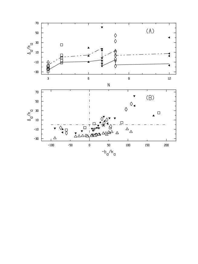
Figure 1: (A) The one-loop normalized threshold corrections ${\Delta_{a}\over k_{a}}$ to the gauge coupling constants are plotted as a function of the orbifold order $N$ for the sixteen orbifold models described in the text. The triangles and squares plotting symbols give the total ${\Delta_{a}\over k_{a}}$ for the various gauge group factors. The back-reaction contributions to ${\Delta_{a}\over k_{a}}$ are shown by points joined by continuous lines. The full gravitational correction $\Delta_{R}$ is shown by points joined by dashed lines. (B) The one-loop normalized threshold corrections are plotted as a function of the normalized slope parameter $-{b_{a}\over k_{a}}$. We denote results for the gauge group factors of $Z_{3}$ orbifolds by open triangles; $Z_{4}$ by open squares; $Z_{6}$ by filled triangles pointing up; $Z_{7}$ by filled triangles pointing down; $Z_{8}$ by open parallelograms; and $Z_{12}$ by filled triangles pointing leftwards.

The results for the orbifolds other than $Z_{3}$ indicate the presence of a residual component $R_{a}$. This appears in a clearer way on plot (B) in figure 1. The signature for a decomposition of $\Delta_{a}$ in terms of only two universal components would appear in this plot as a clustering of the points along a single straight line whose intercept and slope identify with $Y$ and $\Delta$, respectively. The conclusions from figure 1 is that no clear systematic trend towards such a universal behavior is visible on the results. However, for a fixed orbifold order $N$, the deviations $R_{a}$ are quite small and alignments along straight lines are observed. The purest case is that of $Z_{3}$ orbifolds. For the higher-order orbifolds, common trends do appear, such as a positive $\Delta$ (negative $Y$) which increases (decreases) with increasing $N$.

It is interesting to contrast the predictions for the gauge coupling constants against the phenomenologically favored ones. Naively, a reduction of $M^{\prime}_{X}\sim 10^{18}$ down to $M_{GUT}\sim 10^{16}$ would require $\Delta\simeq-10$, while a shift from a dilaton vacuum expectation value set at a strongly coupled regime, say, ${4\pi\over g_{X}^{2}}\sim O(1)$, or at the self-dual point of $S-$duality, $S\to{(4\pi)^{2}\over S}$, to the empirical value, ${4\pi\over{g^{\prime}}_{X}^{2}}\sim 25$, would require $Y\simeq 300$. It appears then that the predicted moduli-independent corrections are much too small, and even of wrong sign for $\Delta$ and $Y$, with respect to a naive perturbative string theory unification scenario. Nevertheless, viable scenarios can be found in association with the other expected mechanisms of an anomalous $U(1)$ threshold and small affine level for $U(1)_{Y}$ [20].

The threshold corrections for the quadratic gravitational interactions arising from the term $\tilde{E}_{2}(\tau)$ in eq.(42) are also shown in plot (A) of figure 1. The zero-mode contribution is again dominated by the anomaly compensating back-reaction contribution from the $-{3\over\pi\tau_{2}}$ term, which numerically coincides with that of the gauge interactions case. The net correction to $\Delta_{R}$ shows some model dependence for orbifold orders $N\geq 6$ and smoothly increases from $-16$ for $Z_{3}$ to $+8$ for $Z_{12}$ orbifolds. Thus, expressed as a shift in the tree level coupling constant, $\delta({4\pi\over g_{X}^{2}})={\Delta_{R}\over 4\pi}$, the threshold correction represents a tiny few percent effect.

3.2 Moduli-dependent threshold corrections

In this section we present a comparison with the moduli-dependent threshold corrections in the quadratic gauge and gravitational interactions. We apply the methods initiated in [3] and further developed in [14] to the curved space-time regularization approach of Section 2. The one-loop contributions from the ${\cal N}=2$ supersymmetric suborbifolds (with an unrotated two-dimensional torus) have a simple representation in terms of a summation involving the right-moving sector massive BPS states, along with an unrestricted sum over the left-moving sector states. The so-called perturbative BPS (Bogomolnyi-Prasad-Sommerfield) states are the stable string modes which saturate the mass bound, ${\alpha^{\prime}\over 4}M_{R}^{2}\geq{p_{R}^{2}\over 2}$, where the ${\cal N}=2$ central charge, $p_{R}$, identifies with the zero-mode momentum of the unrotated two-dimensional torus [73]. The one-loop contributions in the gauge and gravitational coupling constants read:

$$\bigg{[}{(4\pi)^{2}\over k_{a}g_{a}^{2}};{(4\pi)^{2}\over g_{R}^{2}}\bigg{]}=-{1\over 4}\int_{F}{d^{2}\tau\over\tau_{2}^{2}}Z_{W}(\tau,\bar{\tau})(\tau_{2}Z_{\Gamma}(y,\bar{y}))\bigg{[}F_{1}(q)+{F_{2}(q)\over\pi\tau_{2}};F^{g}_{1}(q)+{F_{2}(q)\over\pi\tau_{2}}\bigg{]},$$ (71)

where the partition function for the zero-modes lattice of the internal space fixed two-dimensional torus, denoted $Z_{\Gamma}(y,\bar{y})=\sum q^{p_{L}^{2}/2}\bar{q}^{p_{R}^{2}/2}$, depends on the two complex moduli fields, $y=[y_{+}=T=T_{1}+iT_{2},\ y_{-}=U=U_{1}+iU_{2}]$, parametrizing the coset space, $SO(2,2,R)/SO(2,R)\times SO(2,R)$. A similar procedure to that of Section 2 (separation of the massless modes at the $\tau_{2}\to\infty$ degeneration limiti, subtraction of the field theory one-loop contribution and introduction of the $\overline{DR}$ renormalized conatant) is used to define the threshold corrections, $\Delta_{a},\ \Delta_{R}$. The string theory contributions involve the following periodic Ramond sector traces associated with the so-called new supersymmetry index,

$$[F_{1}(q),\ F_{1}^{g}(q),\ F_{2}(q)] = {1\over\eta^{2}}{i\over 2}Tr_{R}\bigg{(}J_{0}e^{i\pi J_{0}}[8\hat{J}_{a}^{2},\ {E_{2}(\tau)\over 3},\ -1]q^{H}\bar{q}^{\bar{H}}\bigg{)},$$ (72)

$$= \sum_{m\geq-1}^{\infty}[c(m),\ c^{g}(m),\ \hat{c}(m)]q^{m},$$

which are meromorphic functions of $q$, with at most simple poles at the cusp point, $\tau=i\infty$, and Laurent series expansions given by the second line of eq.(72). The zero-mode component, $J_{0}$, of the $U(1)$ current, $J(\bar{z})$, is related to the fermion number operator, $F$, such that, ${i\over 2}Tr_{R}(J_{0}e^{i\pi J_{0}}\cdots)=Tr_{R}((-1)^{F}\cdots)$. All three functions, $F_{1},\ F_{1}^{g},\ F_{2}$, are modular functions for the $SL(2,Z)$ modular group, of weight $0$ for $F_{1},F_{1}^{g}$, and $-2$ for $F_{2}$, except for modular anomalies of the same form as for ${1\over\tau_{2}}$, which cancel exactly in the relevant modular invariant combinations, $[F_{1}+{F_{2}\over\pi\tau_{2}},\quad F_{1}^{g}+{F_{2}\over\pi\tau_{2}}]$. These functions exhibit simple universality properties for the class of non-prime $Z_{N}$ orbifold models associated with decomposable six-dimensional tori, $T^{6}=T^{4}/G\oplus T^{2}$. For the subclass of standard gauge embedding orbifolds, we find by explicit calculation,

$$F_{1}(q) = c(0)\bigg{[}1+{11\over 11088}({E_{6}^{2}-E_{2}E_{4}E_{6}\over\Delta}+720)\bigg{]}=c(0)(1+330q+26400q^{2}+881100q^{3}+\cdots),$$

$$F_{2}(q) = -{4\over|G|\Delta}E_{6}E_{4}={4\over|G|}(-{1\over q}+240+141444q+8529280q^{2}+\cdots),$$

$$F_{1}^{g}(q) = {4\over 3|G|\Delta}E_{6}E_{4}E_{2}={4\over 3|G|}({1\over q}-264-135756q-5117440q^{2}-\cdots),$$ (73)

where $\Delta(\tau)=\eta^{24}(\tau)$ and $E_{2k}(\tau)$ are the Eisenstein series functions, normalized as, $E_{2k}(i\infty)=1$. The model dependence in eq.(73) resides only in the slope parameter coefficients, $b_{a}={c(0)\over 4},\quad b_{R}={c^{g}(0)\over 4}=-{1\over 48}(N_{H}-N_{V}+24)$, and in the orbifold order, $|G|$. ($N_{H},\ N_{V}$ are the numbers of ${\cal N}=2$ hyper and vector supermultiplets, including the dilaton and graviphoton, respectively.) Substituting in eq.(71) and carrying the modular integrals by means of familiar methods [3, 14, 22], one finds the following formula for the threshold corrections in the gauge coupling constants:

$$\Delta_{a} = {c(0)\over 4}[\ln(2T_{2}U_{2})-{\pi\over 3}U_{2}+{\cal K}^{\prime}]-{\pi\over 12}T_{2}(c(0)-24c(-1))+R\sum_{r>0}c(kl)\ln(1-e^{2\pi ix})$$ (74)

$$- {\hat{c}(0)\over 4\pi^{2}U_{2}T_{2}}(\zeta(3)+{2\over\pi}\zeta(4)U_{2}^{3})-{\pi\over 72}T_{2}(\hat{c}(0)-48\hat{c}(-1))-{1\over\pi U_{2}T_{2}}R\sum_{r>0}\hat{c}(kl)P(x),$$

where ${\cal K}^{\prime}=\ln{4\pi e^{3-3\gamma_{E}}\over 9\sqrt{3}}={\cal K}+\ln{e^{2(1-\gamma_{E})}\over 3},\quad\zeta(3)=1.2020569...,\ \zeta(4)={\pi^{4}\over 90},\ \gamma_{E}=0.5772156...$ (Euler-Mascheroni constant); $r=(-l,-k)$ is the lattice vector of the fixed two-dimensional torus, such that the scalar product, $r\cdot y=ky_{+}+ly_{-},$ with the special definition, $x=r\hat{\cdot}y=|R(kT+lU)|+i|I(kT+lU)|$, where $R,I$ mean real and imaginary parts; $r>0$ means ($k>0,l\in Z;$) or ($k=0,l>0$); $P(x)=(Ix)Li_{2}(Q)+{1\over 2\pi}Li_{3}(Q),\ [Q=e^{2\pi ix}]$ with $Li_{j}(Q)=\sum_{p>0}{Q^{p}\over p^{j}}$, the Polylogarithm functions. To translate the automorphic fields notation used here into the string fields notation, one must apply the transformation, $y_{\pm}\to iy_{\pm}$ ($T\to iT,\quad U\to iU$). As functions of $T,U$, the $\Delta_{a}$ are invariant under the modular group, $O(2,2,Z)\sim SL(2,Z)_{T}\times SL(2,Z)_{U}$ which includes the interchange $T\leftrightarrow U$. The representation in eq.(74), which is only valid in the domain $T_{2}>U_{2}$, is transformed when passing through the wall at $T_{2}=U_{2}$, by the substitution $T\leftrightarrow U$.

The formula corresponding to (74) for the gravitational correction $\Delta_{R}$ is obtained by simply changing $c(n)\to c^{g}(n)$, keeping the coefficients $\hat{c}(m)$ unchanged.

The only discrepancy between our result and those found in the approach of [3, 14] resides in a shift of the constant term corresponding to the numerically small difference, ${\cal K}^{\prime}-{\cal K}={\cal K}^{\prime}-\ln{4\pi e^{1-\gamma_{E}}\over\sqrt{27}}=2-2\gamma_{E}-\ln 3\simeq-0.253$. The effective unification scale, incorporating the constant term from the ${\cal N}=2$ sector, $M_{X}^{{}^{\prime}2}=M_{X}^{2}e^{-{\cal K}^{\prime}}={3\over\alpha^{\prime}e^{2(1-\gamma_{E})}2\pi^{2}}={6M_{S}^{2}\over e^{2(1-\gamma_{E})}(4\pi)^{2}}$, is then a factor $3e^{-2(1-\gamma_{E})}\approx 1.29$ larger than that given in [3]. The mismatch originates from the use there of the simple-minded infrared regularization factor, $(1-e^{-N/\tau_{2}})({N\over\tau_{2}})^{\epsilon}$, with the limits, $N\to\infty,\ \epsilon\to 0$. In contrast to our curvature infrared regularization, which is realized by the partition function factor,

$$Z_{W}(\tau,\bar{\tau})\simeq[1+2\phi(\mu)-\phi(2\mu)],\quad\bigg{[}\phi(\mu)=(1-\mu{\partial\over\partial\mu})\sum_{m\neq 0}e^{-{\pi m^{2}\over\mu^{2}\tau_{2}}}\bigg{]}$$ (75)

the regularization prescription in [3] clashes with modular invariance.

The constant, $O(q^{0})$, term in the decomposition of $F_{1}(q)$ in eq.(73), gives rise to the gauge group dependent contribution involving $c(0)$ in eq.(74), which is associated with the subset of the BPS states with $kl=0$, namely, $(k=0,l\in Z)$ or $(k>0,l=0)$. This sums up to, $(\Delta_{a})_{DKL}=b_{a}[\ln(2T_{2}U_{2}|\eta(T)\eta(U)|^{4})+{\cal K}^{\prime}]$, which identifies with the total correction initially discussed by Dixon, Kaplunovsky and Louis [3]. The non-constant terms in $F_{1}(q)$ of $O(q^{n}),\ [n>0]$ which arise from the combination,

$${E_{6}^{2}(\tau)-E_{2}(\tau)E_{4}(\tau)E_{6}(\tau)\over\Delta(\tau)}+720=j(\tau)-{E_{2}(\tau)E_{4}(\tau)E_{6}(\tau)\over\Delta(\tau)}-1008,$$

are associated to the contribution from the subset of states, $(k>0,\ l\in Z)$ in eq.(74). Based on the representation, $j(\tau)-744={1\over q}+196884q+21493760q^{2}+\cdots=\sum_{m\geq-1}c^{j}(m)q^{m},$ and the Borcherds product formula [14], the term involving $j(\tau)$ yields a contribution to $\Delta_{a}$ proportional to $\ln q_{T}^{-1}\prod_{k>0,\ l\in Z}(1-q_{T}^{k}q_{U}^{l})^{c^{j}(kl)}=\ln[j(T)-j(U)]$, where $q_{T,U}=e^{2\pi i[T,U]}$. The singularity at the submanifold $T=U$ mod($SL(2,Z)$ is a reflection of the stringy Higgs mechanism responsible for the enhanced symmetry, $U(1)_{T}\times U(1)_{U}\to SU(3)$, in the gauge group associated with the internal space coordinates of the fixed two-dimensional torus [73]. The absence of singularities in the threshold corrections $\Delta_{a}$, associated with gauge symmetries from the gauge sector space, is due to the compensation by a corresponding singular $\ln(T-U)$ contribution from the remaining terms in $F_{1}(q)$. For the gravitational case, the compensation of the singularity at $T=U$ in $\Delta_{R}$ takes place upon adding the contributions from $F_{1}^{g}$ and $F_{2}(q)$.

A related discussion of the universality properties for the subclass of ${\cal N}=2$ models obtained by toroidal compactification of ${\cal N}=1$ models in six dimensions is given in [34, 37]. Another interesting class of ${\cal N}=2$ compactification models with non-universal behavior is discussed in [36].

Figure 2: The one-loop threshold corrections for decomposable tori models, specialized to the $Z_{4}$ orbifold case, are plotted as a function of $T=T_{1}+iT_{2},U=U_{1}+iU_{2}$ at $T_{1}=U_{1}=0$, with the variables $T_{2},\ U_{2}$ along the horizontal axes. The three plots from left to right show the universal components $\Delta,Y$ for the gauge interactions and $\Delta_{R}$ for the quadratic gravitational interactions.

We shall now present results for the class of models described by eq.(73). In terms of the two-component decomposition, $\Delta_{a}=-b_{a}\Delta+k_{a}Y$, the quantities $\Delta,\ Y$ are then identified with the zero-modes and back-reaction contributions associated with $F_{1}(q)$ and $F_{2}(q)$, respectively. The numerical results are shown in figure 2. The relationship between $T,U$ and the representations of the metric and torsion tensors in the zero-modes lattice basis is given by:

$$T = 2(B_{12}+i\sqrt{detG})=(b+ir_{1}r_{2}\sin\theta),\quad U=(G_{12}+i\sqrt{detG})/G_{11}={r_{2}\over r_{1}}e^{i\theta},$$ (76)

where $2[G_{11},G_{22},\ G_{12},B_{12}]=[r_{1}^{2},\ r_{2}^{2},\ r_{1}r_{2}\cos\theta,\ b]$, such that, $T,b,r_{i}^{2}$ are expressed in units $\alpha^{\prime}=1$. Close to the self-dual points, $T=U=i$, the moduli-dependent corrections are comparable in size with the moduli-independent corrections, but with an opposite negative sign for $\Delta$. For example, at $T_{2}=3,\ U_{2}=4$, one has: $\Delta=-2.17,\ Y=-60.,\ \Delta_{R}=16$. The variations are rather smooth and have a linear power law increase at large $T$ or $U$. At fixed $U$, say, $U=4i$ or ${i\over 4}$, one finds: $\Delta\simeq-0.66|T|,\ Y\simeq-12.7|T|,\ \Delta_{R}\simeq 10.5|T|.$ The dependence on the real parts is weak. Recall that $\Delta,\ \Delta_{R}$ and $Y$ are symmetric under $T\leftrightarrow U$ and that their values for $T,U$ below and above $i$ are connected by the duality transformations, $T\to-{1\over T},\ U\to-{1\over U}$. For large compactification volumes, the correction $\Delta$ has the right sign for a reduced unification scale, and the right magnitude provided that $T\sim O(10)$. The correction $Y$, although of sizeable magnitude, also has a wrong sign to shift the dilaton vacuum expectation value towards weak coupling. The total correction $\Delta_{R}$ in the gravitational case is of opposite sign to (and same magnitude as) that in the gauge case. The associated unification scale, ${M^{\prime}}^{R}_{X}=e^{-\Delta_{R}/bR}M_{X}$, is enhanced (reduced) for negative (positive) $b_{R}$.

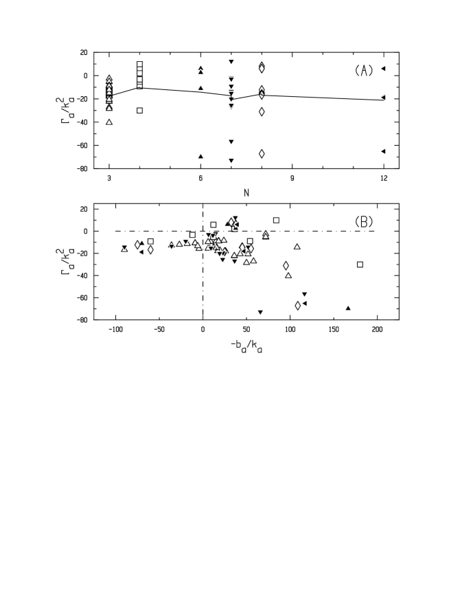
Figure 3: (A) The one-loop threshold corrections to the quartic $F_{a}^{4}$ gauge interactions coupling constants are plotted as a function of the orbifold order $N$ for the sixteen orbifolds described in the text. The triangles and squares plotting symbols give the normalized quantities ${\Gamma_{a}\over k^{2}_{a}}$ for the various gauge group factors in each model. The points joined by continuous lines give the contributions of the two gauge group independent terms. (B) The one-loop normalized threshold corrections are plotted as a function of the normalized slope parameters $-{b_{a}\over k_{a}}$. We denote $Z_{3}$ orbifolds by open triangles; $Z_{4}$ by open squares; $Z_{6}$ by filled triangles pointing up; $Z_{7}$ by filled triangles pointing down; $Z_{8}$ by open parallelograms; and $Z_{12}$ by filled triangles pointing leftwards.

For comparison with [37], where the $Z_{2}\times Z_{2}$ orbifold was considered, we observe that, whereas their function $F_{1}(q)$ has the same formal structure as in our class of models, the decomposition $\Delta_{a}=(b_{a}\Delta-k_{a}Y)_{KKPR}$ there identifies the gauge-dependent term, $(b_{a}\Delta)_{KKPR}$, with our term denoted $(\Delta_{a})_{DKL}$ and the universal term, $-(k_{a}Y)_{KKPR}$, with the remainder contributions from $F_{1}(q)$ and $F_{2}(q)$. Our total results are compatible with those in [34, 37].

3.3 Quartic order gauge interactions

The numerical calculations for the $F^{a4}$ interactions are more intricate than those of the lower-order interactions. Larger number of contributing terms are involved, as can be seen on eq.(43). The various terms contribute more or less equally. We have simply subtracted out the large $\tau_{2}\to\infty$ tails for all terms, except for the two $O(1/\tau_{2}^{2})$ terms, whose contribution to the modular integral is finite.

The results for the moduli-independent threshold corrections obtained for our sample of sixteen orbifold models are shown in plot (A) of figure 3. For a given orbifold order, the corrections $\Gamma_{a}$ are rather widely spread, somewhat more than for $\Delta_{a}$. They cover an interval ranging from $10$ to $-80$. The contributions from the back-reaction (gauge group independent) terms lie near $-20$ and significantly cancel those of the zero-modes.

The corrections $\Gamma_{a}$ include a sizeable part independent of the particular gauge group factor. A dependence on the factor group is also present, as is seen on the plot (B) in figure 3. While a correlation between $\Gamma_{a}$ and the slope parameters is not immediately apparent on the figure, there appears a systematic trend for an increase of the corrections with $-{b_{a}\over k_{a}}$. For a comparison with the tree level coupling constant, we make the bold approximation that one structure only is present, say, that associated with $s_{1}$. The total contribution would read then, $S_{EFF}/F^{a4}\sim s_{1}(e^{-2\Phi}+Z_{1F^{a}})={s_{1}\over 2\pi}({4\pi\over g_{X}^{2}}+{\Gamma_{a}\over 2\pi s_{1}})$. For $\Gamma_{a}\sim O(10)$ and $s_{1}={3\over 128}$, it appears that the one-loop threshold corrections correspond to a large, almost one order of magnitude effect.

4 Discussion and conclusions

The need for an infrared scale parameter which separates the low and high energy theories mass spectra is an inevitable auxiliary item in any description of threshold corrections. Of course, it is always possible to circumvent the infrared regularization by restricting oneself to the consideration of (moduli or matter fields) derivatives of the coupling constants, ${\partial G\over\partial y_{\pm}},\ [G=g_{a}^{2},g_{R^{2}}^{2}]$, as in the calculations of [5, 6], or to gauge group and moduli-dependent components, as in [3]. In so doing, however, one gives up useful information on the absolute size of threshold corrections.

In point quantum field theories, a standard choice for the infrared parameter is the floating off-shell momentum scale used in the renormalization group method. The description here proceeds by equating the summed tree and ultraviolet divergent loop contributions to the unrenormalized coupling constants in the low and high energy theories, after expressing these in terms of the renormalized running coupling constants at the infrared scale, $M$. The threshold corrections emerge then as the boundary condition terms at the ultraviolet decoupling scale $M_{X}$ [74], as is exhibited on the formal equation:

$${1\over G(M_{X})}+b\ln{M\over M_{X}}+\Delta={1\over G(p)}+b\ln{M\over p}.$$

Things differ for string theories because the first-quantized (Polyakov or operator) formalisms are on-shell S-matrix approaches, where the (tadpoles, mass shifts) divergences in the modular variables integrals arise through ${0\over 0}$ ill-defined expressions (see Chapter 8 in [75]). What is most specific about string theory is that infinities are of infrared rather than ultraviolet origin. In particular, the notion of renormalized string theory coupling constants is pointless. Several proposals of off-shell formalisms [76], and of extensions of the space-time dimensional continuation procedure [77], have been been made in the literature. No simple satisfactory method has emerged so far. Thus, to extract the infrared scale logarithmic dependence of the gauge coupling constant, Minahan [1] had to evaluate the world sheet correlator for three gauge bosons, using a prescription for going off the energy shell consistent with conformal and modular invariance. The background field approach stands as one promising alternative approach. In the approximate treatment of Kaplunovsky [2], an infrared cut-off was introduced implicitly, as can be seen by writing his matching formula in the notations of the present paper,

$${(4\pi)^{2}\over g_{a}^{2}(p)}-{(4\pi)^{2}k_{a}\over g_{X}^{2}} - b_{a}\ln{p^{2}\over\Lambda^{2}}-\Delta_{a}=\sum_{i}(I_{i}^{0}-L_{i}^{0})$$ (77)

$$= -b_{a}\bigg{(}\int_{F}{d^{2}\tau\over\tau_{2}}-\int_{0}^{\infty}{dt\over t}C_{\Lambda}(t)\bigg{)}=-b_{a}[1-\gamma_{E}+\ln{2\over\pi\sqrt{27}\Lambda^{2}}].$$

The choice of the ultraviolet cut-off function, $C_{\Lambda}(t)=(1-e^{-t\Lambda^{2}})$, which characterizes $g_{a}(p)$ as the Pauli-Villars renormalized field theory coupling constant, yields the same answer as the $\overline{DR}$ prescription. The infrared divergences at large values of $\tau_{2}$ and $t=\pi\alpha^{\prime}\tau_{2}$, when regularized by a sharp cut-off $\tau_{2}\leq(M^{2}\alpha^{\prime})^{-1}$, mutually cancel out, so that one is led to an effective unification scale $M_{X}$ which coincides with ours in eq.(56). On the other hand, as we already pointed out after eq.(74), for the moduli-dependent threshold corrections, the use of a similar technically inspired cut-off in the modular integrals [3] leads to a different constant term.

The crucial advantage of the infrared regularization by a space-time curvature is that it can be implemented for both the string and field theories using well-defined correspondence rules. The infrared cut-off on the string theory side is the dimensionless Kac-Moody level parameter, $\mu^{2}={1\over k+2}$, while the corresponding parameter on the effective field theory side, $\mu_{e}^{2}={1\over k}$, identifies with the spatial manifold $S^{3}$ radial scale factor. Since all dimensions are set by the string theory tension, the analog of the dimensional floating scale here is $M^{2}={\mu^{2}\over\alpha^{\prime}}$. In fact, by exploiting the representation of the semiwormhole partition function in terms of a $\Gamma(1,1)$ lattice partition function, the analogy can be extended at a deeper level by deriving an infrared renormalization group flow equation for the string theory vacuum functional [22].

The motivations for the finite curvature approach of Kiritsis and Kounnas [22] bear a remote analogy with those which inspired earlier proposals in field theory [78]. These applications rather aimed at formulations of scale invariant theories exhibiting manifest invariance with respect to the conformal transformations group, $O(4,1)$ or $O(5)$. Negative curvature space-time, in particular, was argued to have beneficial effects on the dynamics, for example, by suppressing certain non-perturbative effects [79]. The full implementation of a curvature regularized theory would run into significant technical complications if one needed an explicit construction of the world sheet correlators, as this would entail solving an interacting two-dimensional sigma model. Fortunately, with threshold corrections, one is only concerned with the spectrum of would-be massless states and their degeneracy, an information which is encoded in the partition function.

The use of curved space-time string theory solutions formed from ${\cal N}=4$ superconformal field theory building blocks has desirable features listed in [22]: A free curvature parameter to monitor the decompactification limit; A well-identified classical field theory limit; Preservation of the space-time supersymmetry properties; Solvable marginal deformations to represent covariantly constant gauge and gravitational background fields. The simplest models of type, $M^{(4)}\times K$, where the ${\cal N}=4$ block, $M^{(4)}$, is substituted for the flat space-time, $R^{4}$, allows one to explore the class of phenomenologically viable orbifold compactification models for the internal space $K$. The semiwormhole solution $M^{(4)}=W_{k}^{(4)}$ presents the enormous advantage of the partition function factorizability. The consideration of the other known solutions [27, 28, 52], $M^{(4)}=\Delta_{k}^{(4)}$ or $C_{k}^{(4)}$, may involve a less transparent formalism which has not been developed so far.

The combination of a conformal algebra structure along with a geometrical sigma-model description is the main attraction of the approach of [22]. This completes the approach of [2] by a consistent account for the back-reaction terms, which are essential for ensuring the modular invariance. While the form of these terms for the gauge coupling constants could have been guessed on the basis of modular invariance, a systematic procedure is clearly needed for the higher-derivative interactions.

The reason that only the knowledge of the space-time block partition function is needed in calculating the threshold corrections rests on the conjectured equivalence between the low energy limit of the string theory vacuum functional and the effective action encoding the world sheet conformal symmetry constraints [80]. The dependence on the background fields must then be identical in the string and field theories functionals, up to appropriate field redefinitions. The term by term identification of powers of the background fields uses in an essential way the connection formulas between the vertex operators and the sigma-model deformation parameters. These matching equations provide sets of relations between the string one-loop contributions and the renormalization constants. They can also be interpreted as corrections to the string theory equations of motion involving renormalization contributions to the various interactions. The matching assumption can be viewed as an implementation of the Fischler-Susskind mechanism [62], where the world sheet infrared regulator associated with the size of the world sheet torus handle is replaced by the space-time curvature parameter.

The connection formulas between the string theory and sigma-model deformation parameters follow from a consideration of the mass spectra. However, once the semiwormhole solution is deformed or tensored with a non-trivial internal space, as in $W_{k}^{(4)}\times K$, the dependence of the effective action on the background fields is only valid in the classical limit, corresponding to the leading powers of ${1\over k}$ for a given interaction. The semiwormhole would be an exact quantum solution only for the special model $W_{k}^{(4)}\times R^{6}$, also known as the fivebrane soliton [30]. Thus, unlike the string theory functional dependence on $k$, which is exactly known thanks to the conformal and modular symmetries constraints, the information on the $k-$dependence of the effective action is only limited to the leading powers. This fact is responsible for the restricted predictive power of the approach. The higher orders could possibly be generated perurbatively by solving the string theory equations of motion, which would then involve more detailed information contained in the Green’s functions. To develop the background fields formalism in an order by order in ${1\over k}$ identification would also require a systematic consideration of all the higher-derivative interactions in the effective action. Dealing with these technicalities would make the analysis quite unwieldy, but perhaps not beyond reach.

The implication of our numerical results for the moduli-independent threshold corrections is that these represent small effects for the quadratic order interactions, corresponding to a few percent corrections on the improved coupling constant or scale. Thus, a simple-minded explanation for the standard model gauge coupling constant unification, as being solely due to heavy threshold corrections is ruled out. The new revised results leave the initial conclusions [20, 21] unchanged. The scenarios for perturbative string theory unification appealing to the combined effects of affine algebra levels, anomalous $U(1)$ factor and enhanced threshold corrections from large compactification volumes should continue to provide a viable alternative. However, the last item here may prove less effective, since considerations from string duality indicate the existence of an upper bound on the compactification radius [81], $R\leq{1\over\alpha_{X}M_{P}}$.

The one-loop threshold corrections to the higher-derivative $R^{2}$ gravitational interactions could possibly inform us about the existence of higher-derivative interactions which are not reducible to the topological Gauss-Bonnet combination. Unfortunately, we have been unable to answer this question, because of the technical difficulties in disentangling the three invariant structures. For the quartic order $F^{a4}$ gauge interactions, we also had to restrict consideration to a linear combination of the invariant couplings which remains unknown. Our treatment is also qualitative with respect to the group theory factors and the unresolved mixing with the quadratic gravitational interactions. However, the numerical results here indicate the presence of large moduli-independent threshold corrections relative to the tree level coupling constants.

APPENDIX A

A.1 Expansion of partition function in background fields

We consider the expansion of the deformed theory partition function, $Z(F^{a},R)$, eq.(27), in powers of the the gauge and gravitational field strength parameters, $F^{a},R$, using eq.(20) to describe the perturbed conformal weights. The power expansion up to quartic order is:

$$e^{-4\pi\tau_{2}\delta L_{0}}=1-{{I_{3}\,{\it\bar{Q^{\prime}}}\,t\,R}\over{2\,{\sqrt{{\it K}}}\,{\sqrt{k}}}}+\left({{-\left({I_{3}^{2}}\,t\right)}\over{8\,k}}-{{{{{\it\bar{Q^{\prime}}}}^{2}}\,t}\over{8\,{\it K}}}+{{{I_{3}^{2}}\,{{{\it\bar{Q^{\prime}}}}^{2}}\,{t^{2}}}\over{8\,{\it K}\,k}}\right)\,{R^{2}}$$ (A.1)

$$+ \left({{{I_{3}^{3}}\,{\it\bar{Q^{\prime}}}\,{t^{2}}}\over{16\,{\sqrt{{\it K}}}\,{k^{{3\over 2}}}}}+{{I_{3}\,{{{\it\bar{Q^{\prime}}}}^{3}}\,{t^{2}}}\over{16\,{{{\it K}}^{{3\over 2}}}\,{\sqrt{k}}}}-{{{I_{3}^{3}}\,{{{\it\bar{Q^{\prime}}}}^{3}}\,{t^{3}}}\over{48\,{{{\it K}}^{{3\over 2}}}\,{k^{{3\over 2}}}}}\right)\,{R^{3}}$$

$$+ \left({{{I_{3}^{2}}\,t}\over{32\,k}}+{{{{{\it\bar{Q^{\prime}}}}^{2}}\,t}\over{32\,{\it K}}}+{{{I_{3}^{4}}\,{t^{2}}}\over{128\,{k^{2}}}}+{{{I_{3}^{2}}\,{{{\it\bar{Q^{\prime}}}}^{2}}\,{t^{2}}}\over{64\,{\it K}\,k}}+{{{{{\it\bar{Q^{\prime}}}}^{4}}\,{t^{2}}}\over{128\,{{{\it K}}^{2}}}}-{{{I_{3}^{4}}\,{{{\it\bar{Q^{\prime}}}}^{2}}\,{t^{3}}}\over{64\,{\it K}\,{k^{2}}}}-{{{I_{3}^{2}}\,{{{\it\bar{Q^{\prime}}}}^{4}}\,{t^{3}}}\over{64\,{{{\it K}}^{2}}\,k}}+{{{I_{3}^{4}}\,{{{\it\bar{Q^{\prime}}}}^{4}}\,{t^{4}}}\over{384\,{{{\it K}}^{2}}\,{k^{2}}}}\right)\,{R^{4}}$$

$$+ \left({{-\left({J_{a}^{2}}\,t\right)}\over{8\,{\it k_{a}}}}-{{{{{\it\bar{Q^{\prime}}}}^{2}}\,t}\over{8\,{\it K}}}+{{{J_{a}^{2}}\,{{{\it\bar{Q^{\prime}}}}^{2}}\,{t^{2}}}\over{8\,{\it K}\,{\it k_{a}}}}\right){F_{a}^{2}}+\left({{{J_{a}^{3}}\,{\it\bar{Q^{\prime}}}\,{t^{2}}}\over{16\,{\sqrt{{\it K}}}\,{{{\it k_{a}}}^{{3\over 2}}}}}+{{J_{a}\,{{{\it\bar{Q^{\prime}}}}^{3}}\,{t^{2}}}\over{16\,{{{\it K}}^{{3\over 2}}}\,{\sqrt{{\it k_{a}}}}}}-{{{J_{a}^{3}}\,{{{\it\bar{Q^{\prime}}}}^{3}}\,{t^{3}}}\over{48\,{{{\it K}}^{{3\over 2}}}\,{{{\it k_{a}}}^{{3\over 2}}}}}\right){F_{a}^{3}}$$

$$+ \left({{{J_{a}^{2}}\,t}\over{32\,{\it k_{a}}}}+{{{{{\it\bar{Q^{\prime}}}}^{2}}\,t}\over{32\,{\it K}}}+{{{J_{a}^{4}}\,{t^{2}}}\over{128\,{{{\it k_{a}}}^{2}}}}+{{{J_{a}^{2}}\,{{{\it\bar{Q^{\prime}}}}^{2}}\,{t^{2}}}\over{64\,{\it K}\,{\it k_{a}}}}+{{{{{\it\bar{Q^{\prime}}}}^{4}}\,{t^{2}}}\over{128\,{{{\it K}}^{2}}}}-{{{J_{a}^{4}}\,{{{\it\bar{Q^{\prime}}}}^{2}}\,{t^{3}}}\over{64\,{\it K}\,{{{\it k_{a}}}^{2}}}}-{{{J_{a}^{2}}\,{{{\it\bar{Q^{\prime}}}}^{4}}\,{t^{3}}}\over{64\,{{{\it K}}^{2}}\,{\it k_{a}}}}+{{{J_{a}^{4}}\,{{{\it\bar{Q^{\prime}}}}^{4}}\,{t^{4}}}\over{384\,{{{\it K}}^{2}}\,{{{\it k_{a}}}^{2}}}}\right){F_{a}^{4}}$$

$$+ {{{\rm O}(R)}^{5}}+{{{\rm O}(F_{a})}^{5}}.$$

We have omitted, for simplicity, the mixed power terms, $O(F^{n}R^{m})$, and used the following abbreviations: $\bar{Q}^{\prime}=\bar{Q}+\bar{I}_{3},K=k+2,t=8\pi\tau_{2}$.

A.2 Zero-mode operators

Let us first recall our normalization conventions for the $SU(2)_{k}$ and $U(1)_{k_{a}}$ affine algebras:

$$I_{i}(z)I_{j}(0)\simeq{k\delta_{ij}\over 2z^{2}},\quad J_{a}(z)J_{b}(0)\simeq{k_{a}\delta_{ab}\over 2z^{2}},\quad\bar{Q}_{a}(\bar{z})\bar{Q}_{b}(0)\simeq{\delta_{ab}\over\bar{z}^{2}},$$ (A.2)

and the definition of the conformal weights operators in eq.(12). The zero-mode operators for the Cartan subalgebra of commuting generators act essentially by inserting the charge component as a factor inside the sum representation of the corresponding theta-function or character function. This statement can be schematically expressed as, $\bar{Q}^{2}\to\bar{\vartheta}_{\alpha\beta}^{\prime\prime}\sim\sum p^{2}q^{p^{2}/2},\ \bar{Q}^{4}\to\bar{\vartheta}_{\alpha\beta}^{(iv)}\sim\sum p^{4}q^{p^{2}/2},$ with derivatives operating on $\vartheta_{\alpha\beta}(\nu|\tau)\sim\sum q^{p^{2}/2}e^{2\pi i\nu p}$ as $\partial/(2\pi i\partial\nu)$. More specifically, the action can be expressed as a logarithmic derivative with respect to $q$ or $\bar{q}$ acting on the corresponding determinantal factor which occurs in the partition function $Tr(q^{L_{0}}\bar{q}^{\bar{L}_{0}})$. For the gauge operator zero-mode, using $L_{0}^{gauge}=J_{a}^{2}/k_{a}$, the component decomposition of the world sheet current operator, $J_{a}=\sqrt{k_{a}\over 2}\hat{J}_{a}(z),\ \hat{J}_{a}(z)=\sum_{I=1}^{16}J_{a}^{I}i\partial F^{I}$, normalized as $Tr\hat{J}^{2}_{a}={\psi^{2}\over 2}={1\over 2}$, and the schematic correspondence:

$$J^{2}_{a}\to k_{a}L_{0} = {k_{a}\over 2}2q{d\over dq}={k_{a}\over 2}J_{a}^{I2}\bigg{(}2q{d\over dq}\bigg{)}_{I}={k_{a}\over 2}J_{a}^{I2}\bigg{(}{\partial\over 2\pi i\partial\nu_{I}}\bigg{)}^{2},$$ (A.3)

one derives the general formula:

$$(J_{a}^{2}-{k_{a}\over 8\pi\tau_{2}})\prod_{I=1}^{16}\vartheta^{I}\to{k_{a}\over 2}\big{[}\sum_{I}J_{a}^{I2}(2q{d\over dq})_{I}+\sum_{I\neq J}J_{a}^{I}J_{a}^{J}{\partial^{2}\over(2\pi i)^{2}\partial\nu_{I}\partial\nu_{J}}-{1\over 4\pi\tau_{2}}\big{]}\prod_{I}^{16}\vartheta^{I}(\nu_{I}|\tau)|_{\nu_{I}=0}.$$ (A.4)

The fermionic $SO(8)$ Cartan subalgera helicity generators, $\bar{Q}_{a}=(\bar{Q},\bar{Q}_{i}),\ [i=1,2,3]$ contribute to the conformal weight as, $\bar{L}_{0}=\sum_{a}{\bar{Q}_{a}^{2}\over 2}$, so that their action on on the spinor fields theta-functions factors reads:

$$\bar{Q}^{2} \to 2\bar{q}{d\over d\bar{q}}\ln\bar{\vartheta}[{\bar{\alpha}\atop\bar{\beta}}],\quad\bar{Q}_{i}^{2}\to 2\bar{q}{d\over d\bar{q}}\ln\bar{\vartheta}[{\bar{\alpha}+g_{i}\atop\bar{\beta}+h_{i}}].$$ (A.5)

The space-time orbital helicity generators, $I_{3},\bar{I}_{3}$, for the $SU(2)_{k}$ factor, enter the conformal weight as $L_{0}^{SU(2)_{k}}=\vec{I}^{2}/(k+2)$, which implies that $[\vec{I}^{2},\vec{\bar{I}^{2}}]\to(k+2)[L_{0},\bar{L}_{0}]={(k+2)\over 2}[2q{d\over dq},2\bar{q}{d\over d\bar{q}}]$, operating on the corresponding character function factors, $\chi_{l,k},\bar{\chi}_{l,k}$, in the partition function $X^{\prime}(\mu)$, namely, on the factor $X_{2}$ in the decomposition, $X^{\prime}(\mu)=X_{1}X_{2},\quad[X_{1}=(\sqrt{\tau_{2}}\eta(\tau)\bar{\eta}(\bar{\tau}))^{3}]$, where $X_{1}$ comprises the flat space limit contributions from the zero-modes and oscillator excitations. Simultaneously, we must subtract the free coordinate contributions, $I_{3}^{2}\to{k\over 2}2q{d\over dq}{1\over\eta}$. It is convenient to express the action of $I_{3}^{2},\bar{I}^{2}_{3}$ directly as derivatives acting on $X^{\prime}(\mu)$, so as to exploit the known properties of this function at the various limits. For this purpose, as just stated, we need to correct for the contributions arising from the explicit action of the derivatives on the flat space and oscillator terms in $X_{1}$, and to subtract out the action on the free coordinate oscillator contribution. Using the group symmetry properties, $<I_{i}^{2p+1}>=0,<I_{3}^{2}>={1\over 3}<\vec{I}^{2}>$, and writing,

$$I_{3}^{2}[{X^{\prime}\over\eta}] = {k+2\over\eta}\bigg{[}{1\over 6}(2q{d\over dq}+{1\over 8\pi\tau_{2}}-{1\over 2}(2q{d\over dq})\ln\eta\bigg{]}X^{\prime}+{k\over 2}{X^{\prime}\over\eta}(2q{d\over dq})\ln\eta$$ (A.6)

$$= [{k+2\over 6}2q{d\over dq}X^{\prime}+{k+2\over 8\pi\tau_{2}}X^{\prime}]{1\over\eta}-{X^{\prime}\over\eta}2q{d\over dq}\ln\eta,$$

we find the explicit formulas:

$$\big{[}(\bar{Q}+\bar{I}_{3})^{2}-{k+2\over 8\pi\tau_{2}}\big{]}X^{\prime}(\mu) = \big{[}2\bar{q}{d\over d\bar{q}}\ln{\bar{\vartheta}[{\alpha\choose\beta}]\over\bar{\eta}}+{k+2\over 6}2\bar{q}{d\over d\bar{q}}\big{]}X^{\prime},$$

$$(I_{3}^{2}-{k\over 8\pi\tau_{2}})X^{\prime}(\mu) = \bigg{[}-2q{d\over dq}\ln\eta(q)+{1\over 4\pi\tau_{2}}+{k+2\over 6}2q{d\over dq}\bigg{]}X^{\prime}(\mu)$$

$$= {i\over\pi}[\tilde{E}_{2}(\tau)-{k+2\over 6}\partial_{\tau}]X^{\prime}(\mu).$$

$$\bigg{[}\tilde{E}_{2}(\tau) = \partial_{\tau}\ln\eta(\tau)-{i\over 4\tau_{2}}={1\over 2}\partial_{\tau}\ln(\eta^{2}(\tau)Im(\tau))={i\pi\over 12}(E_{2}(\tau)-{3\over\pi\tau_{2}}),$$

$$E_{2}(\tau) = {12\over i\pi}\partial_{\tau}\ln\eta=1-24\sum_{n=1}^{\infty}\sigma_{1}(n)q^{n}\bigg{]}$$ (A.7)

In the sum representation of the zeta-function regularized Eisenstein function, $\sigma_{1}(n)=\sum_{d|n}d$ denotes the sum of the divisors of $n$. The antiholomorphic quantities are deduced by complex conjugation.

The treatment of higher powers of the zero-modes operators follows from similar considerations. One finds:

$$I_{3}^{4}[X^{\prime}] = {1\over 5}\bigg{[}({k+2\over 2})^{2}X_{1}(2q{d\over dq})^{2}X_{2}-({k\over 2})^{2}X^{\prime}(\mu)(2q{d\over dq})^{2}\ln{1\over\eta^{3}}\bigg{]}$$ (A.8)

$$= -{1\over 5\pi^{2}}\bigg{\{}({k+2\over 2})^{2}\bigg{[}\partial_{\tau}^{2}+3({\eta^{{}^{\prime}2}\over\eta^{2}}-{\eta^{\prime\prime}\over\eta}-{1\over 8\tau_{2}^{2}})$$

$$+ 6({i\over 4\tau_{2}}-{\eta^{\prime}\over\eta})\partial_{\tau}\bigg{]}+{3k^{2}\over 4}({\eta^{\prime\prime}\over\eta}-{\eta^{{}^{\prime}2}\over\eta^{2}})\bigg{\}}X^{\prime}(\mu)$$

$$\to -{3\over 5}X^{\prime}(2q{d\over dq})^{2}\ln\eta={3X^{\prime}\over 5\pi^{2}}({\eta^{\prime\prime}\over\eta}-{\eta^{\prime 2}\over\eta^{2}}),$$

where $\eta^{\prime}=\partial_{\tau}\eta(\tau)$ and we expressed the angle averaging by means of the classical formula, $I_{3}^{4}\to\vec{I}^{2}/5$. The result appearing on the last line in eq.(A.8) is obtained by selecting the $O(k^{0})$ term and dropping all terms proportional to powers of $k$ or $(k+2)$. The corresponding formula for the total angular momentum projection is,

$$(\bar{Q}+\bar{I}_{3})^{4}=\bar{Q}^{4}+\bar{I}_{3}^{4}+6\bar{Q}^{2}\bar{I}_{3}^{2}\to{\bar{\vartheta}_{\alpha\beta}^{(iv)}\over\bar{\vartheta}_{\alpha\beta}}-6{\bar{\vartheta}_{\alpha\beta}^{{}^{\prime\prime}}\over\bar{\vartheta}_{\alpha\beta}}(2\bar{q}{d\over d\bar{q}}\ln\bar{\eta})-{3\over 5}(2\bar{q}{d\over d\bar{q}})^{2}\ln\bar{\eta}.$$ (A.9)

The gauge zero-mode operators action is given by:

$$J^{a4} \to \sum_{I}J_{I}^{a4}\partial_{IIII}^{4}+\sum_{I\neq J}(3J_{I}^{a2}J_{J}^{a2}\partial_{II}^{2}\partial_{JJ}^{2}+4J_{I}^{a3}J_{J}^{a}\partial_{III}^{3}\partial_{J})$$ (A.10)

$$+ \sum_{I\neq J\neq K}6J_{I}^{a2}J_{J}^{a}J_{K}^{a}\partial_{II}^{2}\partial_{JK}^{2}+\sum_{I\neq J\neq K\neq L}J_{I}^{a}J_{J}^{a}J_{K}^{a}J_{L}^{a}\partial^{4}_{IJKL}.$$

where the derivatives $\partial_{I}={\partial\over 2\pi i\partial\nu_{I}}$ operate on the $E_{8}\times E_{8}$ Cartan subalgebra components of the fermionic gauge fields determinantal factors, $\vartheta[{\alpha\atop\beta}](\nu_{I}|\tau)$.

A.3 Modular integrals

To evaluate the modular integrals in the limit $\mu\to 0$, it is convenient to use the representation, $X(\mu)=Z_{T}(\mu)-Z_{T}(2\mu)$, while truncating the winding modes summation to the $n=0$ term,

$$Z_{T}(\mu)=\sqrt{\tau_{2}}\sum_{(m,n)\in Z^{2}}e^{2\pi imn\tau_{1}}e^{-\pi\tau_{2}(m^{2}\mu^{2}+{n^{2}\over\mu^{2}})}\simeq\sqrt{\tau_{2}}\vartheta_{3}(i\tau_{2}\mu^{2})={1\over\mu}\vartheta_{3}({1\over-i\tau_{2}\mu^{2}}),$$

where the equation in the last step is deduced by means of the duality transformation $\tau\to-1/\tau$. An important observation is that in the difference $Z_{T}(\mu)-Z_{T}(2\mu)$, the contribution from the $m=0$ term in the momentum modes sum cancels out, so that there occurs an overall damping factor, $e^{-\pi\tau_{2}\mu^{2}}$, as required by the regularization. If one simply factored out the $e^{-\pi\mu^{2}\tau_{2}}$ dependence, this would prevent one from simplifying the integrands by using the duality transformation. Nevertheless, a convenient approximation for the integrals $J_{1},K_{1}$, valid up to small corrections $O(e^{-1/\mu^{2}}),O(e^{-\Lambda^{2}/\mu^{2}})$, can be obtained by using the two truncations detailed in the following steps:

$$X(\mu) \simeq \sqrt{\tau_{2}}e^{-\pi\tau_{2}\mu^{2}}\sum_{m\neq 0}e^{-\pi\tau_{2}(m^{2}-1)}-(\mu\to 2\mu),$$ (A.11)

$$\simeq \sqrt{\tau_{2}}e^{-\pi\tau_{2}\mu^{2}}{1\over\mu\sqrt{\tau_{2}}}[\vartheta_{3}({1\over-i\tau_{2}\mu^{2}})-1]-(\mu\to 2\mu)$$

$$\simeq {1\over\mu}e^{-\pi\tau_{2}\mu^{2}}-(\mu\to 2\mu),$$

where the first truncation amounts to the substitution, $(m^{2}-1)\to m^{2}$, and the second to retain the leading term in the limit $\mu\to 0$. One can now evaluate the integral analytically,

$$J_{1} = 4\pi\mu^{2}{\partial\over\partial\mu}\bigg{[}{1\over\mu}\int_{-{1\over 2}}^{1\over 2}d\tau_{1}\int_{\sqrt{1-\tau_{1}^{2}}}^{\infty}{d\tau_{2}\over\tau_{2}}e^{-\pi\tau_{2}\mu^{2}}-(\mu\to 2\mu)\bigg{]}$$ (A.12)

$$= -4\pi\mu^{2}{\partial\over\partial\mu}\bigg{[}{1\over\mu}\int_{-{1\over 2}}^{1\over 2}d\tau_{1}Ei(-\pi\mu^{2}(1-\tau_{1}^{2})^{1\over 2}-(\mu\to 2\mu)\bigg{]}$$

$$= 2\pi[\gamma_{E}-3+\ln({\pi\sqrt{27}\over 8}\mu^{2})],$$

where $Ei$ is the Exponential integral function and we have used: $\int_{-{1\over 2}}^{1\over 2}dx\ln(1-x^{2})=(3\ln 3-2-2\ln 2),\quad Ei(\infty)\to 0,\quad Ei(z)\simeq\gamma_{E}+\ln z+O(z)$. A similar approximation applies to the corresponding field theory integral,

$$K_{1}\simeq 4\pi\mu_{e}^{2}{\partial\over\partial\mu_{e}}\bigg{[}{1\over\mu_{e}}\int_{1\over\pi\Lambda^{2}}^{\infty}{dt\over t}e^{-\pi t\mu^{2}}-(\mu_{e}\to 2\mu_{e})\bigg{]}=2\pi[\gamma_{E}-2+\ln{\mu_{e}^{2}\over 4\Lambda^{2}}].$$ (A.13)

A useful approximation for the integrals, $J_{n},K_{n},$ for $(n=2,3)$, is again to truncate the winding modes $n\neq 0$, but to retain all the momentum modes, $m\in Z$, while extending the range of the modular integral for $m>0$ to the entire upper half-strip. The procedure, valid up to the same exponential accuracy as quoted above, can be described as:

$$\int_{F}{d^{2}\tau\over\tau_{2}^{n}}Z_{T}(\mu) \simeq {1\over\mu}\bigg{[}\int_{F}{d^{2}\tau\over\tau_{2}^{n}}+\int_{-{1\over 2}}^{1\over 2}d\tau_{1}\int_{0}^{\infty}{d\tau_{2}\over\tau_{2}^{n}}(\vartheta_{3}({1\over-i\tau_{2}\mu^{2}})-1)\bigg{]}$$ (A.14)

$$= {1\over\mu}\bigg{(}f_{n}+2\mu^{2n-2}\pi^{1-n}\Gamma(n-1)\zeta(2n-2)\bigg{)}.$$

$$\bigg{[}f_{n}=[{\pi\over 3},{1\over 2}\ln 3],\quad[n=2,3]\bigg{]}$$

References

• [1] J. Minahan, Nucl. Phys. B298, 36 (1988)
• [2] V. S. Kaplunovsky, Nucl. Phys. B307, 145 (1988); Erratum B382, 436 (1992)
• [3] L. Dixon, V. S. Kaplunovsky and J. Louis, Nucl. Phys. B355, 649 (1991)
• [4] I. Antoniadis, K. S. Narain and T. Taylor, Phys. Lett. B276, 37 (1991)
• [5] I. Antoniadis, E. Gava and K. S. Narain, Phys. Lett. B283, 209 (1992); Nucl. Phys. B383, 93 (1992)
• [6] I. Antoniadis, E. Gava, K. S. Narain and T. Taylor, Nucl. Phys. B407, 706 (1993); ibidem B413, 162 (1994)
• [7] J. L. Derendinger, S. Ferrara, C. Kounnas, and F. Zwirner, Nucl. Phys. B372, 145 (1992)
• [8] L. E. Ibãnéz and D. Lüst, Nucl. Phys. B382, 305 (1992)
• [9] G. L. Cardoso and B. Ovrut, Nucl. Phys. B392, 315 (1993); ibidem B369, 351 (1992)
• [10] P. Mayr and S. Stieberger, Nucl. Phys. B407, 725 (1993)
• [11] D. Bailin, A. Love, W. A. Sabra and S. Thomas, Phys. Lett. B320, 21 (1994); Mod. Phys. Lett. A9, 67 (1994)
• [12] V. Kaplunovsky and J. Louis, Nucl. Phys. B422, 57 (1994); ibidem B444, 191 (1995)
• [13] G. Lopes Cardoso, G. Curio and D. Lüst, hep-th/9608154
• [14] J. A. Harvey and G. Moore, Nucl. Phys. B463, 315 (1996)
• [15] I. Antoniadis, J. Ellis, R. Lacaze and D. V. Nanopoulos, Phys. Lett. B268, 188 (1991); L. Dolan and J. T. Liu, Nucl. Phys. B387, 86 (1992)
• [16] S. Kalara, J.L. Lopez and D. V. Nanopoulos, Phys. Lett. B269, 84 (1991)
• [17] K. R. Dienes and A. E. Faraggi, Phys. Rev. Lett. 75, 2646 (1995); Nucl. Phys. B457, 409 (1995); A. E. Faraggi, Phys. Lett. B302, 202 (1993)
• [18] L. Ibãnéz, D. Lüst and G. G. Ross, Phys. Lett. B272, 251 (1991)
• [19] P. Mayr, H.-P. Nilles and S. Stieberger, Phys. Lett. B317, 53 (1993)
• [20] M. Chemtob, Phys. Rev.D53, 3920 (1996)
• [21] K. R. Dienes, hep-th/9602045, to appear in Phys. Reports
• [22] E. Kiritsis and C. Kounnas, Nucl. Phys. B442, 472 (1995); Nucl. Phys. (Proc. Suppl.) 41B, 331 (1995)
• [23] C. G. Callan, J. Harvey and A. Strominger, String Theory and Quantum Gravity 1991, eds. I. Klebanov et al., Proc. Trieste Spring School (World Scientific, Singapore, 1992); G. Horowitz, String Theory and Quantum Gravity 1992, ed. J. Harvey et al., Proc. Trieste Spring school (World Scientific, Singapore, 1993)
• [24] A. Giveon, M. Porrati, and E. Rabinovici, Phys. Reports, 244, 77 (1994)
• [25] I. Bars and D. Nemeschansky, Nucl. Phys. 348, 89 (1991); I. Bars and K. Sfetsos, Phys. Rev. D46, 4510 (1992)
• [26] I. Bars, Phys. Lett. B293, 315 (1992)
• [27] E. Kiritsis, C. Kounnas and D. Lüst, Int. J. Mod. Phys. A9, 1361 (1994)
• [28] C. Kounnas, Phys. Lett. B321, 26 (1994)
• [29] C. Kounnas, M. Porrati and B. Rostand, Phys. Lett. B258, 61 (1991)
• [30] C. G. Callan, J. Harvey, and A. Strominger, Nucl. Phys. B359, 611 (1991)
• [31] J. Ellis, P. Jetzer, and L. Mizrachi, Nucl. Phys. B303, 1 (1988)
• [32] N. Sakai and Y. Tanii, Nucl. Phys. B287, 457 (1987); M. Abe, H. Kubota and N. Sakai, Nucl. Phys. B306, 405 (1988)
• [33] E. Kiritsis and C. Kounnas, Nucl. Phys. B456, 699 (1995); Nucl. Phys. (Proc. Suppl.) 45B, 207 (1996)
• [34] P. M. Petropoulos and J. Rizos, hep-th/9601037, Phys. Lett. B374, 49 (1996)
• [35] P. M. Petropoulos, hep-th/9605012, 5th Hellenic school and workshops on elementary particle physics, Corfu, Greece, 3-24 September 1995
• [36] E. Kiritsis, C. Kounnas, P. M. Petropoulos and J. Rizos, hep-th/9605011, 5th Hellenic school and workshops on elementary particle physics, Corfu, Greece, 3-24 September 1995
• [37] E. Kiritsis, C. Kounnas, P. M. Petropoulos and J. Rizos, hep-th/9606087, Phys. Lett.B385, 87 (1996)
• [38] E. Kiritsis, C. Kounnas, P. M. Petropoulos and J. Rizos, hep-th/9608034, Nucl. Phys. B483, 141 (1997)
• [39] K. S. Stelle, Phys. Rev. D16, 953 (1977)
• [40] B. Zwiebach, Phys. Lett. B156, 315 (1985)
• [41] A. Hindawi, B. A. Ovrut, and D. Waldram, Phys. Rev. D53, 5583 (1996)
• [42] A. Hindawi, B. A. Ovrut, and D. Waldram, Phys. Lett. B381, 154 (1996); Nucl. Phys. B476, 175 (1996)
• [43] S. Theisen, Nucl. Phys. B263, 687 (1986)
• [44] S. Cecotti, S. Ferrara, L. Girardello, A. Pasquinucci, and M. Porrati, Int. J. Mod. Phys. A3, 1675 (1988)
• [45] G. Lopes Cardoso, D. Lüst, and B. A. Ovrut, Nucl. Phys. B436, 65 (1995)
• [46] J. Harvey, G. Moore, hep-th/9611197
• [47] K. Förger, B. A. Ovrut, S. J. Theisen, and D. Waldram, preprint UER-664T, Phys. Lett. B388, 512 (1996)
• [48] J. Lykken, FERMILAB-PUB-96/070-T, hep-th/9603133, Phys. Rev. D54, 3693 (1996)
• [49] D. Gross and E. Witten, Nucl. Phys. B277, 1 (1986)
• [50] W. Lerche, B. Nilsson, and A. Schellekens, Nucl. Phys. B289, 609 (1987); W. Lerche, B. Nilsson, A. Schellekens, and N. Warner, Nucl. Phys. B299, 91 (1988); W. Lerche, Nucl. Phys. B308, 102 (1988)
• [51] A. A. Tseytlin, Nucl. Phys. B467, 383 (1996); C. Bachas and E. Kiritsis, CERN-TH/96-153, hep-th/9611205
• [52] I. Antoniadis, S. Ferrara and C. Kounnas, Nucl. Phys. B421, 343 (1994)
• [53] D. Gepner and E. Witten, Nucl. Phys. B 278, 493 (1986)
• [54] C. Itzykson, H. Saleur, and J.-B. Zuber, Conformal invariance and Applications to Statistical Mechanics (World Scientific, Singapore, 1988)
• [55] S. Hassan and A. Sen, Nucl. Phys. B405, 143 (1993)
• [56] E. Kiritsis and A. Giveon, Nucl. Phys. B411, 487 (1994)
• [57] P. Mayr and S. Stieberger, Nucl. Phys. B412, 502 (1994)
• [58] P. Ginsparg, Phys. Lett. B197, 139 (1987)
• [59] D. J. Gross and J. H. Sloan, Nucl. Phys. B291, 41 (1987)
• [60] A. A. Tseytlin, Phys. Lett. B176, 92 (1986); Nucl. Phys. B276, 391 (1986); R. R. Metsaev and A. A. Tseytlin, Nucl. Phys. B293, 385 (1987)
• [61] W. Siegel, Phys. Lett. B84, 193 (1979); I. Antoniadis, C. Kounnas and K. Tamvakis, Phys. Lett. B119, 377 (1982)
• [62] W. Fischler and L. Susskind, Phys. Lett. B171, 383 (1986); ibidem, B173, 262 (1986); J. Polchinski, Nucl. Phys. B307, 61 (1988)
• [63] S. M. Christensen and M. Duff, Phys. Lett. B76, 571 (1978); L. Ibanez and D. Lüst, Nucl. Phys. B382, 305 (1992)
• [64] N. D. Birrell and P. C. W. Davies, Quantum fields in curved space-time (Cambridge University Press, Cambridge, 1982)
• [65] J. Atick, L. Dixon, and A. Sen, Nucl. Phys. B292, 109 (1987)
• [66] M. Dine, N. Seiberg, and E. Witten, Nucl. Phys. B 289, 589 (1987); M. Dine and C. Lee, Nucl. Phys. B 336, 317 (1990)
• [67] U. Amaldi, W. de Boer, and H. Fürstenau, Phys. Lett. B260, 447 (1991); J. Ellis, S. Kelley and D. Nanopoulos, Phys. Lett. B260, 131 (1991); P. Langacker, “Precision Tests of the Standard Electroweak model” (World Scientific, 1995, Singapore)
• [68] E. Witten, hep-th/9602070, Nucl. Phys. B471, 135 (1996)
• [69] A. Font, L. E. Ibanez, F. Quevedo, and A. Sierra, Nucl. Phys. B331, 421 (1990)
• [70] H. B. Kim and J. E. Kim, Phys. Lett. B300, 343 (1993)
• [71] Y. Katsuki, T. Kobayashi, N. Ohtsubo, Y. Ono, and K. Tanioka, Nucl. Phys. B341, 611 (1990)
• [72] J. A. Casas, A. de la Macorra, M. Mondragón, and C. Muñoz, Phys. Lett. B247, 50 (1990)
• [73] G. L. Cardoso, D. Lust, and T. Mohaupt, Nucl. Phys. 432, 64 (1994); ibidem B450, 115 (1995); G. L. Cardoso, G. Curio, D. Lust, T. Mohaupt, S.-J. Rey, Nucl.Phys. B464, 18 (1996)
• [74] S. Weinberg, Phys. Lett. B91, 51 (1980)
• [75] M. Green, J. Schwarz, and E. Witten, Superstring theory, (Cambridge University Press, 1987)
• [76] Z. Bern, D. A. Kosower, and K. Roland, Nucl. Phys. B334, 309 (1990); Z. Bern and D. A. Kosower, Nucl. Phys. B379, 451 (1992)
• [77] M. B. Green, J.H. Schwarz, and L. Brink, Nucl. Phys. B198, 472 (1982)
• [78] S. L. Adler, Phys Rev. D6, 3445 (1972); ibidem D8, 2400 (1973); R. Jackiw and C. Rebbi, Phys. Rev. D14, 517 (1976)
• [79] C. G. Callan and F. Wilczek, Nucl. Phys. B340, 366 (1990)
• [80] R. R. Metsaev and A. A. Tseytlin, Nucl. Phys. B298, 111 (1988)
• [81] E. Caceres, V. S. Kaplunovsky, and I. M. Mandelberg, hep-th/9606036