Abstract

The one-loop effective potential for gauge models in static de Sitter space at finite temperatures is computed by means of the $\zeta$–function method. We found a simple relation which links the effective potentials of gauge and scalar fields at all temperatures.

In the de Sitter invariant and zero-temperature states the potential for the scalar electrodynamics is explicitly obtained, and its properties in these two vacua are compared. In this theory the two states are shown to behave similarly in the regimes of very large and very small radii $a$ of the background space. For the gauge symmetry broken in the flat limit ($a\rightarrow\infty$) there is a critical value of $a$ for which the symmetry is restored in both quantum states.
Moreover, the phase transitions which occur at large or at small $a$ are of the first or of the second order, respectively, regardless the vacuum considered. The analytical and numerical analysis of the critical parameters of the above theory is performed. We also established a class of models for which the kind of phase transition occurring depends on the choice of the vacuum.

PACS number(s): 04.62.+v; 11.10.Wx; 05.70.Fh;

e-mail: denardo@na.infn.it; dfursaev@phys.ualberta.ca; miele@na.infn.it

1 Introduction

The aim of this paper is to investigate the properties of the finite-temperature (FT) effective potential of the gauge models in the de Sitter space. The temperature $\beta^{-1}$ is introduced as the temperature of quantum fields which are in thermal equilibrium in the static de Sitter coordinates. Thus, the corresponding quantum state is determined by the Green function which is periodical along the time coordinate of the static frame with period $i\beta$. This enables one to use the Euclidean formulation of the theory. In particular, one can define the partition function $Z_{\beta}$ for arbitrary $\beta$ as a functional integral, where the fields configurations belong to the spherical domain $S^{4}_{\beta}$ with conical singularities on the Euclidean horizon.

There are at least two motivations for this work. The first one is to obtain the one-loop effective potential on such non-trivial spaces like $S^{4}_{\beta}$ in an analytical form. This is a continuation of the pioneering studies by Shore [1] and Allen [2, 3] which investigated the effective actions on hyperspheres $S^{4}$. Furthermore, the paper extends the results of Ref.[4] concerning the scalar fields, to more interesting gauge models with spontaneous symmetry breaking. A second motivation is related to the possible application of these results to cosmological problems since the exponentially expanding phase of the early universe [5] is described by the de Sitter geometry. Our analysis has become possible after the spectrum of vector Laplacians on singular $d$-spheres has been found explicitly in Ref.[6].

In this paper a special attention is paid to calculation and comparison of the effective potentials for two physically relevant quantum states: the de Sitter invariant (dSI) and the zero-temperature (ZT) states. They both can be considered as possible vacua in quantum field theory in the de Sitter space.

The dSI state resembles the Poincaré invariant vacuum of the Minkowski space-time since it preserves the symmetry of the de Sitter space. The corresponding temperature is equal to $(\beta_{H})^{-1}=(2\pi a)^{-1}$, where $a$ denotes the de Sitter radius [7] and the Euclidean section of the de Sitter space is the hypersphere $S^{4}$. In analogy with black hole physics this temperature can be called the Hawking temperature. In the Gibbons–Hawking path integral [8] the Euclidean gravitational action with a positive cosmological constant has the extremum on a 4–sphere $S^{4}$. Thus, the choice of dSI state has a natural explanation in the semi-classical treatment of the quantum cosmology. For this reason the one-loop effective action for quantum fields on $S^{4}$ has been studied in a number of works [2]-[4], [9, 10]. In particular, some authors [3, 9, 10] investigated the phase structure of the GUT models with respect to the value of the de Sitter radius $a$.

The dSI vacuum is analogous to the Hartle–Hawking vacuum [11] introduced for quantum fields around an eternal black hole. From this point of view the zero–temperature state ($\beta\rightarrow\infty$) in the de Sitter space is analogous to the Boulware vacuum [12]. The properties of this state are much less investigated, and we use here the explicit expressions of the effective potential to see how the choice of the vacuum affects the phase structure of the gauge theories with spontaneous symmetry breaking.

The paper is organized as follows. We briefly discuss in Section 2 why the Euclidean functional integral on the spherical domains $S^{4}_{\beta}$ can be interpreted as a partition function in the static de Sitter space. The FT effective potential for gauge models is computed with the $\zeta$–function method in Section 3. In Section 4 we compare the symmetry breaking mechanisms at different values of $a$ in the two vacua for models of scalar electrodynamics. Summary of the results is given in Section 5. Technical details concerning the derivation of the $\zeta$–function are left for Appendix.

2 Partition function

In the static coordinates the line element of the de Sitter space with radius $a$ can be written in the form

$$ds^{2}=\cos^{2}\chi dt^{2}-a^{2}(d\chi^{2}+\sin^{2}\chi d\theta_{1}^{2}+\sin^{2}\chi\sin^{2}\theta_{1}d\theta_{2}^{2})~{}~{}~{},$$ (2.1)

where $-\infty<t<+\infty$, $|\chi|\leq\pi/2$, and $0\leq\theta_{1},\theta_{2}\leq\pi$. The above coordinates (2.1) cover only a part of the space. One can consider a Killing vector field generating a one–parameter group of isometries, subgroup of SO(1,4). Then coordinates (2.1) can be related to the time–like part of the Killing field associated with the translations along the time $t$. This region is restricted by the Killing horizon where the Killing field is null. It also coincides with the event horizon for the observers with coordinates $\chi=0$.

Let $G(x,x^{\prime})$ be a scalar Green function in the de Sitter space-time for dSI state (its some explicit expressions can be found in [13]–[15]). This function is periodic when the time coordinates of points $x$ or $x^{\prime}$ are independently increased by $i\beta_{H}$ [7] where $\beta_{H}=2\pi a$. Thus the Euclidean Green function

$$G^{E}(\tau-\tau^{\prime},u,u^{\prime})=iG(i(\tau-\tau^{\prime}),u,u^{\prime})~{}~{}~{},$$ (2.2)

which is obtained from $G$ with the help of a Wick rotation, is defined on a 4-sphere $S^{4}$ with the line element

$$ds^{2}=\cos^{2}\chi d\tau^{2}+a^{2}(d\chi^{2}+\sin^{2}\chi d\theta_{1}^{2}+\sin^{2}\chi\sin^{2}\theta_{1}d\theta_{2}^{2})~{}~{}~{},$$ (2.3)

where $0\leq\tau\leq\beta_{H}$. Note that because of the periodicity property in imaginary time the function $G(x,x^{\prime})$ can be interpreted as a Green function for a canonical ensemble at temperature $\beta_{H}^{-1}$. The physical meaning behind this interpretation is that any freely moving observer experiences the dSI state as a thermal bath at temperature $\beta_{H}^{-1}$, see Ref.[7].

A natural generalization of $G(x,x^{\prime})$ is a Green function $G_{\beta}(x,x^{\prime})$ in the de Sitter space which is periodic in imaginary time with an arbitrary period $\beta$. Functions of this kind can be constructed from $G(x,x^{\prime})$ with the help of a reperiodization formula suggested by Dowker [16, 17]. One can interpret $G_{\beta}(x,x^{\prime})$ as a Green function of a canonical ensemble of particles in the static part (2.1) of de Sitter space at temperature $\beta^{-1}$. It is also possible to introduce the Euclidean function $G_{\beta}^{E}(x,x^{\prime})$ by using a definition analogous to Eq.(2.2). The space where $G_{\beta}^{E}(x,x^{\prime})$ is set on is a spherical domain $S^{4}_{\beta}$, which is described by the metric (2.3) of the 4-sphere, but now with period $\beta$ along $\tau$.

The main property of $S^{4}_{\beta}$ is that it has conical singularities at the points $\chi=\pm\pi/2$, near which the space looks as $S^{2}\times C_{\beta}$, where $C_{\beta}$ is a cone with deficit angle $2\pi(1-\beta/\beta_{H})$.

Let us consider now the functional integral

$$Z_{\beta}=\int[D\phi]e^{-I_{E}[\phi,g_{\mu\nu}]}~{}~{}~{},$$ (2.4)

where $I_{E}[\phi,g_{\mu\nu}]$ is the classical Euclidean action for the fields $\phi$ on $S^{4}_{\beta}$, $g_{\mu\nu}$ is the metric tensor defined by Eq.(2.3) and $[D\phi]$ is a covariant integration measure. The function $G_{\beta}^{E}$ can be obtained from this integral in the standard way. For instance, for a real scalar field $\phi$ it reads

$$G_{\beta}^{E}(x,x^{\prime})=Z_{\beta}^{-1}\int[D\phi]\phi(x)\phi(x^{\prime})e^{-I_{E}[\phi,g_{\mu\nu}]}~{}~{}~{}.$$ (2.5)

It follows from (2.4) and (2.5) that integral $Z_{\beta}$ is analogous to a statistical-mechanical partition function $\mbox{Tr}~{}e^{-\beta\hat{H}}$ of a canonical ensemble of particles at temperature $\beta^{-1}$. Thus we will call $Z_{\beta}$ partition function and use it for the definition of the effective potential in the theory. The corresponding quantum states will be called FT states. Some justification of this way of doing is that at $\beta=\beta_{H}$ the integral $Z_{\beta}$ defines the quantum theory and effective potential in the dSI state. It should be noted, however, that in case of the Killing horizons $Z_{\beta}$ and statistical-mechanical partition function $\mbox{Tr}~{}e^{-\beta\hat{H}}$ are not completely equivalent .

Their relation was investigated in the case of black hole geometries with the aim to establish the statistical explanation of the black hole entropy, see for instance Ref.s[18]–[21]. We will not dwell on this issue further since it is not relevant for our purposes.

It has to be also mentioned that in the presence of the Killing horizon the function $G^{E}_{\beta}(x,x^{\prime})$ does not have the Hadamard form [22] when $\beta\neq\beta_{H}$. In this case the stress energy tensor of a quantum field has a non-integrable divergence on the horizon of the chosen static coordinate system [16]. As was discussed in Ref.[23], this property alone may be not sufficient to exclude FT states as unphysical, since the computation of the stress tensor neglects the backreaction effects. Such effects are very strong near the horizon and a reliable computation requires a nonperturbative approach which is not still developed. However, a non-Hadamard form of $G^{E}_{\beta}(x,x^{\prime})$ is not an obstacle for the definition of the partition function (2.4). The conical singularities of $S^{4}_{\beta}$ result only to a number of additional ultraviolet divergent terms in the effective action $-\ln Z_{\beta}$ and one can use the standard renormalization procedure to give a meaning to the integral (2.4). We will discuss this later.

3 Effective potential

3.1 The model

We focus now on the definition and computation of the FT effective potential for the scalar electrodynamics in the de Sitter space. A similar computation has been done before by Shore [1] and Allen [2] for the dSI state. We restrict our analysis to the abelian theories because the generalization to non-abelian case, as was shown in Ref.[3], is almost straightforward.

Let us consider the model of a complex self-interacting scalar field $\phi$, which interacts also with an abelian gauge field $A_{\mu}$. The classical Lorentzian action reads

$$I\left[A_{\mu},\phi\right]=\int{\sqrt{-g}~{}dx^{4}~{}\left[-{1\over 4}F_{\mu\nu}F^{\mu\nu}+{1\over 2}\left(D_{\mu}\phi\right)\left(D^{\mu}\phi\right)^{*}-V(\phi)\right]}~{}~{}~{},$$ (3.1)

where

$$F_{\mu\nu} = \nabla_{\mu}A_{\nu}-\nabla_{\nu}A_{\mu}~{}~{}~{},$$ (3.2)

$$D_{\mu}\phi = \partial_{\mu}\phi-ieA_{\mu}\phi~{}~{}~{},$$ (3.3)

$$V(\phi) = {1\over 2}\left(m^{2}+\xi R\right)\phi^{*}\phi+{\lambda\over 4!}\left(\phi^{*}\phi\right)^{2}~{}~{}~{}.$$ (3.4)

The coupling $e$ stands for the electric charge, $\lambda$ is the constant of the self-interaction, which is assumed to be positive, and $\xi$ denotes the coupling to the scalar curvature $R=12/a^{2}$. According to Eq.(2.4), the partition function $Z_{\beta}$ for this model at an arbitrary temperature $\beta^{-1}$ is the Euclidean functional integral

$$Z_{\beta}=\int[D\phi]~{}[DA_{\mu}]~{}[D\bar{c}]~{}[Dc]\exp\left\{-I_{E}\left[A_{\mu},\phi,\bar{c},c\right]\right\}~{}~{}~{},$$ (3.5)

$$I_{E}\left[A_{\mu},\phi,\bar{c},c\right]=I_{E}\left[A_{\mu},\phi\right]+\triangle I\left[A_{\mu},\phi\right]+I_{\mbox{gh}}\left[\bar{c},c,\phi\right]~{}~{}~{},$$ (3.6)

where all the fields are given on the spherical domain $S_{\beta}^{4}$, Eq.(2.3). The functional $I_{E}$ denotes the Euclidean form of action (3.1). The term $\triangle I$ is a gauge fixing term, $\bar{c}$, $c$ are the corresponding ghost fields and $I_{\mbox{gh}}[\bar{c},c,\phi]$ is their action. The explicit form of these quantities will be fixed below.

We will use the effective potential method to study the phase transitions in the theory (3.1). The symmetry breaking in our model is characterized by the average value $<\hat{\phi}>_{\beta}$ of the scalar field in the given FT state. If this average does not depend on time and on the spatial coordinates $\chi,\theta_{1},\theta_{2}$, the effective potential $V_{\mbox{eff}}(\varphi,\beta)$ can be introduced by following the method of Ref.[4]. To this aim one can separate the field $\phi$ onto a constant part $\varphi$ (which can be chosen real) and the excitations $\phi^{\prime}=\phi_{1}+i\phi_{2}$

$$\phi=\varphi+\phi^{\prime}=\varphi+\phi_{1}+i\phi_{2}~{}~{}~{}.$$ (3.7)

The effective potential is determined by the relation

$$Z_{\beta}=\int d\varphi~{}\exp\left\{-\beta{\cal V}V_{\mbox{eff}}(\varphi,\beta)\right\}~{}~{}~{},$$ (3.8)

$$\exp\left\{-\beta{\cal V}V_{\mbox{eff}}(\varphi,\beta)\right\}=\int[D\phi^{\prime}]~{}[DA_{\mu}]~{}[D\bar{c}]~{}[Dc]\exp\left(-I_{E}\left[A_{\mu},\phi^{\prime},\bar{c},c\right]\right)~{}~{}~{},$$ (3.9)

where $\beta{\cal V}=\frac{4}{3}\pi a^{3}\beta$ is the volume of $S^{4}_{\beta}$. Note that the integral (3.8) is the usual integral.

As was shown in Ref.[4], a point $\varphi_{0}$ where $V_{\mbox{eff}}(\varphi,\beta)$ has a minimum, coincides with the one-loop value of the average $<\hat{\phi}>_{\beta}$. The real part of $V_{\mbox{eff}}(\varphi,\beta)$ is a sum of the classical potential energy $V(\varphi)$ and a quantum correction. If the field configuration $\varphi_{0}$ is unstable, then $V_{\mbox{eff}}(\varphi_{0},\beta)$ has a nonvanishing imaginary part which determines the decay probability of this configuration.

To compute $V_{\mbox{eff}}$ with the help of Eq.(3.9) it is suitable to use the t’Hooft gauge with the gauge fixing term

$$\Delta I\left[A_{\mu},\phi\right]={1\over 2}\alpha\int_{S^{4}_{\beta}}{\sqrt{g}~{}dx^{4}~{}\left[\nabla_{\mu}A^{\mu}-\alpha^{-1}e\varphi\phi_{2}\right]^{2}}~{}~{}~{},$$ (3.10)

where $\alpha$ is an arbitrary parameter. Then, by expanding the classical potential to the second order in $\phi_{1}$ and $\phi_{2}$, one gets

$$I_{E}\left[A_{\mu},\phi\right]+\triangle I\left[A_{\mu},\phi\right]=\frac{1}{2}\int_{S^{4}_{\beta}}\left[A^{\mu}_{T}\left(\triangle^{(T)}_{\mu\nu}+e^{2}\varphi^{2}g_{\mu\nu}\right)A^{\nu}_{T}+\alpha A^{\mu}_{L}\left(-\nabla_{\mu}\nabla_{\nu}+\alpha^{-1}e^{2}\varphi^{2}g_{\mu\nu}\right)A^{\nu}_{L}\right.$$

$$\left.+\phi_{1}(-\nabla^{2}+V^{\prime\prime}(\varphi))\phi_{1}+\phi_{2}(-\nabla^{2}+\alpha^{-1}e^{2}\varphi^{2}+\varphi^{-1}V^{\prime}(\phi))\phi_{2}\right]\sqrt{g}d^{4}x~{}~{}~{},$$ (3.11)

where $A^{\mu}_{T}$ and $A^{\mu}_{L}=\nabla_{\mu}\chi$ are the transverse and longitudinal component of the vector field, respectively, and $\triangle^{(T)}_{\mu\nu}=-g_{\mu\nu}\nabla^{\sigma}\nabla_{\sigma}+R_{\mu\nu}$ is the transverse Hodge-deRham operator.

Hereafter, we will be interested in the situation where the one-loop quantum effects can change significantly the form of the classical potential. As was pointed out by Coleman and Weinberg [24], who investigated the model (3.1) in the flat space, one has to assume to this aim that the gauge coupling $e^{4}$ is of the order of $\lambda$. In this case the quantum corrections due to the gauge fields will be comparable with the classical potential. On the other hand, to provide the convergence of the perturbation expansions one has to assume that $\lambda\ll 1$. In this case one can safely neglect the contributions to the effective potential of the scalar loops which will be proportional to $\lambda^{2}\ll e^{4}$.

3.2 Representation for the potential

In order to simplify the computations it is convenient to choose the Landau gauge for which $\alpha\rightarrow\infty$. Then the contribution of the ghost fields does not depend on the average value of the field $\varphi$, and since it does not affect the symmetry breaking in the model, it can be neglected. As was explained above, the contribution of the scalar excitations can be neglected as well. After that one arrives to the obvious result

$$V_{\mbox{eff}}(\varphi,\beta)=V(\varphi)+{3\over 8\pi a^{3}\beta}\log\mbox{det}\left[\mu^{-2}\left(\Delta^{(T)}_{\mu\nu}+e^{2}\varphi^{2}g_{\mu\nu}\right)\right]~{}~{}~{}.$$ (3.12)

Further we make use of the $\zeta$–function regularization method [25] which defines the determinant of an operator $A$ with eigen-values $\lambda_{n}$

$$\log\mbox{det}\left[\mu^{-2}A\right]=-\zeta^{\prime}_{A}(0)-\zeta_{A}(0)\log\mu^{2}~{}~{}~{}$$ (3.13)

in terms of the generalized $\zeta_{A}$–function

$$\zeta_{A}(z)=\sum_{n,(\lambda_{n}\neq 0)}\lambda_{n}^{-z}~{}~{}~{}$$ (3.14)

and its derivative $\zeta^{\prime}_{A}(z)=d\zeta_{A}(z)/dz$. An arbitrary mass parameter $\mu$ is introduced in Eq.(3.13) to keep the right dimensionality.

Let us note that the $\zeta$–function method automatically gives a finite expression for the quantum determinants. The last term in the right hand side of Eq.(3.13) corresponds to the finite counterterms which are always present after renormalization. The conical singularities are known to introduce additional ultraviolet divergences, see for instance Ref’s [26, 27]. The renormalization on manifolds with conical singularities has been discussed recently in a number of papers [26, 28]-[33],[6].

In the case of the Hodge-deRham operator all one-loop divergences which are linear in the conical deficit angle, as shown in Ref.[6], are removed under standard renormalization of the gravitational couplings [34] in the bare gravitational action. The renormalization of the remaining divergences of order $(\beta-\beta_{H})^{2}$ in the deficit angle or higher is more involved, and requires additional counterterms in the effective action. These terms have the form of integral invariants defined on the singular surface [30]. The values of the additional couplings cannot be predicted in the theory, and so to simplify the analysis we will assume that these couplings in $V_{\mbox{eff}}$ are absent.

The definition and representation of the $\zeta$–function $\zeta^{(T)}(z)$ for the transverse Hodge-deRham operator is given in Appendix A. It is convenient to parametrize this function of $z$, in terms of the parameters $\beta$ and $\sigma\equiv\frac{1}{4}-e^{2}a^{2}\varphi^{2}$. Thus, Eq.(3.12) reads

$$V_{\mbox{eff}}(\varphi,\beta)=V(\varphi)-{3\over 8\pi a^{3}\beta}\left[{d\over dz}\zeta^{(T)}\left(0,\beta,\sigma\right)+\zeta^{(T)}\left(0,\beta,\sigma\right)\log\mu^{2}a^{2}\right]~{}~{}~{}.$$ (3.15)

Our key result, whose derivation is given in the Appendix A, is that on $S^{4}_{\beta}$ the $\zeta$-function $\zeta^{(T)}\left(z,\beta,\sigma\right)$ of the vector operator $a^{2}\Delta^{T}_{\mu\nu}+g_{\mu\nu}(\frac{1}{4}-\sigma)$ and the $\zeta$–function $\zeta^{(0)}\left(z,\beta,\sigma\right)$ of the scalar operator $-a^{2}\nabla^{2}+9/4-\sigma$ are related in a simple way, see Eq.(A.8). In particular, one can show with the help of Eqs.(A.9), (A.10) and (A.12) that for arbitrary $\beta$

$${d\over dz}\zeta^{(T)}\left(0,\beta,\sigma\right) = 3{d\over dz}\zeta^{(0)}\left(0,\beta,\sigma\right)-2\left(\int_{{3\over 2}}^{{3\over 2}+\sqrt{\sigma}}+\int_{{3\over 2}}^{{3\over 2}-\sqrt{\sigma}}\right)\left({3\over 2}-u\right)\psi(u)du$$ (3.16)

$$- 4\zeta^{\prime}_{R}\left(-1,{3\over 2}\right)~{}~{}~{},$$

$$\zeta^{(T)}\left(0,\beta,\sigma\right)=3\zeta^{(0)}\left(0,\beta,\sigma\right)+{11\over 12}-\sigma~{}~{}~{},$$ (3.17)

where $\psi(u)\equiv\Gamma^{\prime}(u)/\Gamma(u)$ is the Digamma–function [35]. Thus, the quantum correction $V^{g}_{\mbox{eff}}$ to the potential due to gauge fields and the correction $V^{s}_{\mbox{eff}}$ from the scalars are related in the universal way

$$V^{g}_{\mbox{eff}}(\sigma,\beta)=3V^{s}_{\mbox{eff}}(\sigma,\beta)+\beta^{-1}\Omega(\sigma)~{}~{}~{},$$ (3.18)

where the function $\Omega(\sigma)$ is temperature independent

$$\Omega(\sigma) = {3\over 4\pi a^{3}}\left[\left(\int_{{3\over 2}}^{{3\over 2}+\sqrt{\sigma}}+\int_{{3\over 2}}^{{3\over 2}-\sqrt{\sigma}}\right)\left({3\over 2}-u\right)\psi(u)du\right.$$ (3.19)

$$- \left.4\zeta^{\prime}_{R}\left(-1,{3\over 2}\right)+\frac{1}{2}\left(\sigma-{11\over 12}\right)\log\mu^{2}a^{2}\right]~{}~{}~{}.$$

Hence, the study of the effective potential (3.15) is reduced to the investigation of the scalar functional $V^{s}_{\mbox{eff}}(\sigma,\beta)$ which has been done in Ref.[4]. Let us note, however, that even the structure of $V^{s}_{\mbox{eff}}(\sigma,\beta)$ is rather complicated and in general one may rely only on numerical calculations.

What is interesting is that $V^{s}_{\mbox{eff}}(\sigma,\beta)$ can be found in an analytical form in the two most interesting limits: in the dSI state and in the ZT state. We make use of this fact to consider the phase transitions in the gauge model at different values of the de Sitter radius and compare the phase structures of the theory in these two cases.

3.3 DeSitter-invariant state

We assume that the renormalized mass of the field $\varphi$ is zero and so the classical potential in Eq.(3.15) is

$$V(\varphi)=\frac{1}{2}\xi R\varphi^{2}+{\lambda\over 4!}\varphi^{4}~{}~{}~{},$$ (3.20)

with $R={12/a^{2}}$. Then the expression for the potential, which follows from Eq.(A.13), is

$$V_{\mbox{eff}}(\varphi,\beta_{H})=\frac{1}{2}\xi R\varphi^{2}+{\lambda\over 4!}\varphi^{4}-{3\over(4\pi)^{2}a^{4}}\left[\frac{1}{3}e^{2}a^{2}\varphi^{2}+\frac{1}{4}e^{4}a^{4}\varphi^{4}-{19\over 192}\right.$$

$$+2\zeta_{R}^{\prime}\left(-3,\frac{3}{2}\right)-\frac{9}{2}\zeta_{R}^{\prime}\left(-1,\frac{3}{2}\right)-\left(\int_{{3\over 2}}^{{3\over 2}+\sqrt{\sigma}}+\int_{{3\over 2}}^{{3\over 2}-\sqrt{\sigma}}\right)u\left(u-{3\over 2}\right)(u-3)\psi(u)du$$

$$\left.+\left(\frac{1}{4}e^{4}a^{4}\varphi^{4}+e^{2}a^{2}\varphi^{2}+{19\over 30}\right)\log\mu^{2}a^{2}\right]~{}~{}~{}.$$ (3.21)

One can also define the energy $E$ and the entropy $S$ of the quantum fields at the Hawking temperature. Thus, by making use of (A.13), we find

$$E={4\pi a^{3}\over 3}{\partial\over\partial\beta}\left[\beta V_{\mbox{eff}}\right]|_{\beta=\beta_{H}}={4\pi a^{3}\over 3}\left(\frac{1}{2}\xi R\varphi^{2}+{\lambda\over 4!}\varphi^{4}\right)+{3\over 4\pi a}\left[-\frac{1}{8}e^{4}a^{4}\varphi^{4}-{2\over 9}e^{2}a^{2}\varphi^{2}\right.$$

$$-{19\over 180}\left.+{1\over 12}(e^{4}a^{4}\varphi^{4}+2e^{2}a^{2}\varphi^{2})\left(\psi\left(\frac{3}{2}+\sqrt{\sigma}\right)+\psi\left(\frac{3}{2}-\sqrt{\sigma}\right)-\log\mu^{2}a^{2}\right)\right]~{}~{}~{}.$$ (3.22)

The entropy $S$ of the quantum field in the dSI state is defined as $S=2\pi a(E-V_{\mbox{eff}})$ and its expression follows from Eqs. (3.21) and (3.22).

3.4 Zero-temperature state

As it follows from Eq.(A.17), the effective potential in this case reads

$$V_{\mbox{eff}}(\varphi,\beta=\infty)=\frac{1}{2}\xi R\varphi^{2}+{\lambda\over 4!}\varphi^{4}-{3\over(4\pi)^{2}a^{4}}\left[{1\over 12}e^{4}a^{4}\varphi^{4}-{11\over 12}e^{2}a^{2}\varphi^{2}+{317\over 192}\right.$$

$$-6\zeta_{R}^{\prime}\left(-3,\frac{3}{2}\right)+\frac{3}{2}\zeta_{R}^{\prime}\left(-1,\frac{3}{2}\right)+3\left(\int_{\frac{1}{2}}^{\frac{1}{2}+\sqrt{\sigma}}+\int_{\frac{1}{2}}^{\frac{1}{2}-\sqrt{\sigma}}\right)u\left(u-\frac{1}{2}\right)(u-1)\psi(u)du$$

$$-3\sqrt{{1\over 4}-e^{2}a^{2}\varphi^{2}}\left(\int_{\frac{1}{2}}^{\frac{1}{2}+\sqrt{\sigma}}-\int_{\frac{1}{2}}^{\frac{1}{2}-\sqrt{\sigma}}\right)u\left(u-1\right)\psi(u)du$$

$$\left.+\left(\frac{1}{4}e^{4}a^{4}\varphi^{4}+\frac{1}{4}e^{2}a^{2}\varphi^{2}-{1\over 40}\right)\log\mu^{2}a^{2}\right]~{}~{}~{}.$$ (3.23)

It is interesting to note that the quantum correction to the potential due to gauge fields at zero temperature has the same form of the correction due to the scalar fields multiplied by factor 3, see Eq.(3.18).

3.5 Flat limit

By taking into account that for $z\gg 1$

$$\mbox{Re}~{}\psi\left(\frac{3}{2}+iz\right)=\log z+{11\over 24}z^{-2}-{127\over 960}z^{-4}+O(z^{-8})~{}~{}~{},$$ (3.24)

$$\mbox{Re}~{}\psi\left(\frac{1}{2}+iz\right)=\log z-{1\over 24}z^{-2}-{7\over 960}z^{-4}+O(z^{-8})~{}~{}~{},$$ (3.25)

one can check that the energy density $(4\pi a^{3}/3)^{-1}E$ and the effective potentials $V_{\mbox{eff}}(\varphi,\beta_{H})$ and $V_{\mbox{eff}}(\varphi,\beta=\infty)$ coincide in the limit $a\rightarrow\infty$ with the effective potential in the Minkowski vacuum $V_{\mbox{Mink}}$

$$V_{\mbox{Mink}}(\varphi)={\lambda\over 4!}\varphi^{4}+{3e^{4}\over 64\pi^{2}}\varphi^{4}\left[\log\left({e^{2}\varphi^{2}\over\mu^{2}}\right)-\frac{3}{2}\right]~{}~{}~{}.$$ (3.26)

The last expression enables one to fix the unknown constant $\mu$ in terms of the physical parameters.

The effective potential (3.26) has a minimum at a non-zero value $\varphi=\varphi_{0}$ where

$$\varphi_{0}^{2}={\mu^{2}\over e^{2}}\exp\left(1-{8\pi^{2}\lambda\over 9e^{4}}\right)~{}~{}~{}.$$ (3.27)

Thus the quantum state is characterized by a field configuration with the non-zero average $<\hat{\phi}>\simeq\varphi_{0}$, where the gauge symmetry is spontaneously broken and the gauge field becomes a vector boson with the mass $M=e|\varphi_{0}|$. The potential (3.26), written in terms of the parameter $M$, reads

$$V_{\mbox{Mink}}(\varphi)={3e^{4}\over 64\pi^{2}}\varphi^{4}\left[\log{e^{2}\varphi^{2}\over M^{2}}-\frac{1}{2}\right]~{}~{}~{}.$$ (3.28)

It coincides with the Coleman-Weinberg expression [24]. The result that in the flat limit dSI and ZT states coincide with the Minkowski vacuum is not surprising. In this limit the de Sitter group converts into the Poincaré one and the Hawking temperature vanishes.

3.6 Limit of large curvatures

It is also interesting to compare the form of potentials (3.21) and (3.23) in the opposite limit, when the curvature of the space-time is very large, namely $e^{2}a^{2}\varphi^{2}\ll 1$. Since we are interested in the phase transitions, terms in the potential which do not depend on $\varphi$ are irrelevant. Hence, from now on it is more convenient to deal with the difference $V_{\mbox{eff}}(\varphi,\beta)-V_{\mbox{eff}}(0,\beta)$ which vanishes for $\varphi=0$.

By taking into account Eq.(3.21) one can easily prove that the dominant contribution for the large curvature at $\beta=\beta_{H}$ is

$$V_{\mbox{eff}}(\varphi,\beta_{H})-V_{\mbox{eff}}(0,\beta_{H}) \simeq {3e^{2}\varphi^{2}\over 16\pi^{2}a^{2}}\left[P+{19\over 6}-2\gamma-\log a^{2}M^{2}\right]$$ (3.29)

$$+ {3e^{4}\varphi^{4}\over 64\pi^{2}}\left[3-2\gamma-\log a^{2}M^{2}\right]~{}~{}~{},$$

where

$$P={32\pi^{2}\xi\over e^{2}}-{8\pi^{2}\lambda\over 9e^{4}}-\frac{3}{2}~{}~{}~{},$$ (3.30)

and $\gamma=.5772..$ is the Euler constant. As far as the ZT state is concerned, one can prove the analogous formula

$$V_{\mbox{eff}}(\varphi,\beta=\infty)-V_{\mbox{eff}}(0,\beta=\infty) \simeq {3e^{2}\varphi^{2}\over 64\pi^{2}a^{2}}\left[Q+K-\log a^{2}M^{2}\right]$$ (3.31)

$$+ {3e^{4}\varphi^{4}\over 64\pi^{2}}\left[K+{20\over 3}-\log a^{2}M^{2}\right]~{}~{}~{},$$

where

$$Q={128\pi^{2}\xi\over e^{2}}-{8\pi^{2}\lambda\over 9e^{4}}+{14\over 3}~{}~{}~{},$$ (3.32)

$$K=12\int_{0}^{1/2}\left({1\over 4}-z^{2}\right)\left[\psi\left({1\over 2}+z\right)+\psi\left({1\over 2}-z\right)\right]~{}dz=-5.97011....~{}~{}~{}.$$ (3.33)

Equations (3.29) and (3.31) show that in the limit when the de Sitter curvature is large the potentials are different but have similar structures.

4 Symmetry breaking

In order to compare phase transitions in the scalar electrodynamics (3.1) in dSI and ZT states we rewrite expressions (3.21) and (3.23) in the following dimensionless form

$$A_{1}(x,y)={64\pi^{2}\over 3M^{4}}\left[V_{\mbox{eff}}(\varphi,\beta_{H})-V_{\mbox{eff}}(0,\beta_{H})\right]=4\frac{x}{y}\left(P+{13\over 6}-\log y\right)$$

$$-x^{2}\log y+{4\over y^{2}}\left(\int_{\frac{3}{2}}^{{3\over 2}+\sqrt{\sigma}}+\int_{\frac{3}{2}}^{{3\over 2}-\sqrt{\sigma}}\right)u\left(u-{3\over 2}\right)(u-3)\psi(u)du~{}~{}~{},$$ (4.1)

$$A_{2}(x,y)={64\pi^{2}\over 3M^{4}}\left[V_{\mbox{eff}}(\varphi,\beta=\infty)-V_{\mbox{eff}}(0,\beta=\infty)\right]$$

$$=\frac{x}{y}(Q-\log y)+x^{2}\left(\frac{2}{3}-\log y\right)-{12\over y^{2}}\left(\int_{\frac{1}{2}}^{\frac{1}{2}+\sqrt{\sigma}}+\int_{\frac{1}{2}}^{\frac{1}{2}-\sqrt{\sigma}}\right)u\left(u-\frac{1}{2}\right)(u-1)\psi(u)du$$

$$+{12\over y^{2}}\sqrt{{1\over 4}-xy}\left(\int_{\frac{1}{2}}^{\frac{1}{2}+\sqrt{\sigma}}-\int_{\frac{1}{2}}^{\frac{1}{2}-\sqrt{\sigma}}\right)u(u-1)\psi(u)du~{}~{}~{}.$$ (4.2)

Here

$$x={e^{2}\varphi^{2}\over M^{2}}~{}~{}~{},~{}~{}~{}y=a^{2}M^{2}~{}~{}~{},~{}~{}~{}\sigma=\frac{1}{4}-xy~{}~{}~{},$$ (4.3)

and the renormalization parameter $\mu$ has been expressed, according to Eq.(3.27), in terms of the vector boson mass as $\mu^{2}=M^{2}\exp\left({8\pi^{2}\lambda\over 9e^{4}}-1\right)$. Interestingly, all the information about the constants $e^{2}$, $\lambda$ and $\xi$ of the considered model is contained in the parameters $P$ and $Q$ defined in Eqs.(3.30) and (3.32), respectively.

For arbitrary values of constants $e^{2}$, $\lambda$ and $\xi$ the parameters $P$ and $Q$ are independent. They can be related to each other only in the case of the minimal coupling $\xi=0$.

We consider now the phase structure of the theory in the limit of large and small curvatures of the de Sitter space, where it can be investigated analytically.

4.1 Phase transitions at small curvatures

In this limit $e^{2}a^{2}\varphi^{2}=xy\gg 1$ and one has

$$A_{1}(x,y)=x^{2}\left(\log x-\frac{1}{2}\right)+4\frac{x}{y}\left(\log x+P+\frac{3}{2}\right)~{}~{}~{},$$ (4.4)

$$A_{2}(x,y)=x^{2}\left(\log x-\frac{1}{2}\right)+\frac{x}{y}\left(\log x+Q-{14\over 3}\right)~{}~{}~{}.$$ (4.5)

Eq.(4.4) coincides with the result of Ref.[2]. As was shown in Ref.[2] the symmetry breaking in this limit in dSI state is characterized by first order phase transitions. Under such transitions, when the curvature radius $a$ reduces to a critical value $a_{c}$, the mass of the vector boson changes discontinuously from a value $M_{c}=e\varphi_{c}$ to zero. By comparing Eqs. (4.4) and (4.5) one can see that the effective potential at zero temperature has a similar structure, so in this case one may expect an analogous behavior.

Let $x_{c}$ and $y_{c}$ be critical values of parameters $x$ and $y$ in the point of the phase transition. They are related to the critical radius $a_{c}$ and mass $M_{c}$ as follows

$$x_{c}={M_{c}^{2}\over M^{2}}~{}~{}~{},~{}~{}~{}y_{c}=a_{c}^{2}M^{2}$$ (4.6)

where, as before, $M$ is the mass of the vector boson in the Minkowski space-time. In the given approximation the values of $x_{c}$ and $y_{c}$, with $x_{c}>0$, can be found explicitly. They must satisfy the following conditions

$$\left.{d\over dx}A_{i}(x,y)\right|_{x=x_{c},y=y_{c}}=0~{}~{}~{},$$ (4.7)

$$A_{i}(x_{c},y_{c})=0~{}~{}~{},$$ (4.8)

which can be resolved. For dSI state the results coincide with those of Ref.[2]

$$M_{c}^{2}=M^{2}\exp\left[~{}{-\frac{5}{2}-P\over 1+P+\sqrt{P^{2}-4}}~{}\right]~{}~{}~{},$$ (4.9)

$$a_{c}^{2}=2M_{c}^{-2}\left[~{}P+\sqrt{P^{2}-4}~{}\right]~{}~{}~{}.$$ (4.10)

For the zero temperature we find the following critical mass $\tilde{M}_{c}$ and radius $\tilde{a}_{c}$

$$\tilde{M}_{c}^{2}=M^{2}\exp\left[~{}{\frac{11}{3}-Q\over Q-\frac{31}{6}+\sqrt{\left(Q-\frac{37}{6}\right)^{2}-4}}~{}\right]~{}~{}~{},$$ (4.11)

$$\tilde{a}_{c}^{2}=\frac{1}{2}\tilde{M}_{c}^{-2}\left[~{}Q-\frac{37}{6}+\sqrt{\left(Q-\frac{37}{6}\right)^{2}-4}~{}\right]~{}~{}~{}.$$ (4.12)

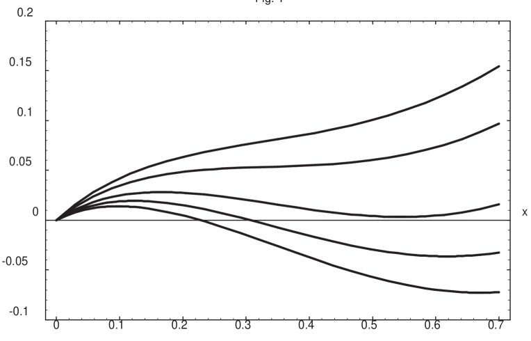
Figure 1: The above curves, from the higher to the lower, represent the function $A_{1}(x,y)$ for $P=10$ and $\sqrt{y}=7.4$, $7.8$, $8.49$, $9$ and $9.5$, respectively (see Ref. [2]). The critical value of de Sitter radius ($\sqrt{y}\approx 8.49$) corresponds to the first order phase transition.

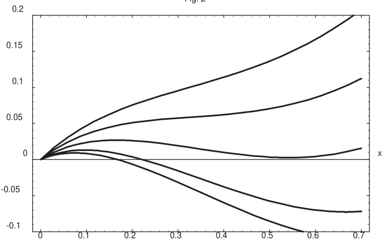
Figure 2: The curves, from the higher to the lower, illustrate $A_{2}(x,y)$ for $Q=16$ and $\sqrt{y}=3.5$, $3.8$, $4.2$, $4.7$ and $5$, respectively. The first order phase transition takes place at $\sqrt{y}\approx 4.2$.

Eqs. (4.9) and (4.10) are valid for $P\geq 2$, and Eqs. (4.11) and (4.12) for $Q\geq 49/6$. Thus we can conclude that in the limit of small curvatures and for the given values of $P$ and $Q$ the dSI and ZT states have qualitatively similar properties. In both cases one has first order phase transitions, but with different values of critical radii and masses. These properties are shown in Figures 1 and 2, where the functions $A_{1}(x,y)$ and $A_{2}(x,y)$ are evaluated for $P=10$ and $Q=16$, respectively. The numerical computations of the critical parameters are in agreement with expressions (4.9)-(4.12).

4.2 Phase transitions at large curvatures

We can use in this regime asymptotics (3.29) and (3.31). As one can see from these equations, the terms proportional to $\varphi^{2}$ change the sign from positive to negative when $a$ becomes larger than a critical value $a_{c}$. In this case to have the symmetry breaking in the theory at $a>a_{c}$ the terms $\varphi^{4}$ in (3.29) and (3.31) have to be positive. When $a$ becomes smaller than $a_{c}$ the mass of the vector boson gradually vanishes. This situation corresponds to second order phase transitions.

The critical radius $a_{c}$ in dSI state is [2]

$$a_{c}^{2}=M^{-2}\exp\left\{P+{19\over 6}-2\gamma\right\}~{}~{}~{}.$$ (4.13)

In order to have a second order phase transition one must ensure that the coefficient of the $\varphi^{4}$ term in (3.29) is positive. By substituting (4.13) in Eq.(3.29) we find that the above condition is satisfied [2] for

$$3-2\gamma-\log a_{c}^{2}M^{2}=-P-\frac{1}{6}>0\Longrightarrow P<-\frac{1}{6}~{}~{}~{}.$$ (4.14)

The value $P=P_{cr}=-1/6$ represents in fact a critical boundary which separates the models of the scalar electrodynamics with different kinds of phase transition. For models with $P$ above $P_{cr}$ the system undergoes first order phase transitions, whereas for models with $P$ below $P_{cr}$ one has second order phase transitions. The value of $P_{cr}$ is also confirmed by the numerical analysis.

A similar expression for the critical radius $\tilde{a}_{c}$ at zero temperature can be found from Eq.(3.31)

$$\tilde{a}_{c}^{2}=M^{-2}\exp\left\{Q+K\right\}~{}~{}~{}.$$ (4.15)

The difference between the values of the critical radii can be estimated by their ratio

$${\tilde{a}_{c}^{2}\over a_{c}^{2}}=\exp\left({96\pi^{2}\xi\over e^{2}}+K+3+2\gamma+{16\pi^{2}\over e^{2}}\right)~{}~{}~{}.$$ (4.16)

It depends only on $\xi$ and $e^{2}$, and for $\xi\gg e^{2}$ one can conclude that $\tilde{a}_{c}\gg a_{c}$. For the minimal coupling ($\xi=0$) $\tilde{a}_{c}^{2}/a_{c}^{2}\simeq 1.63$.

In the case of ZT state the critical value $Q_{cr}$ can be determined as well. By substituting Eq.(4.15) in the coefficient of the quartic term of Eq.(3.31) one gets

$$K+\frac{20}{3}-\log\tilde{a}_{c}^{2}M^{2}=\frac{20}{3}-Q>0\Longrightarrow Q<\frac{20}{3}~{}~{}~{}.$$ (4.17)

Thus $Q_{cr}=20/3$ and it is confirmed by the numerical computations.

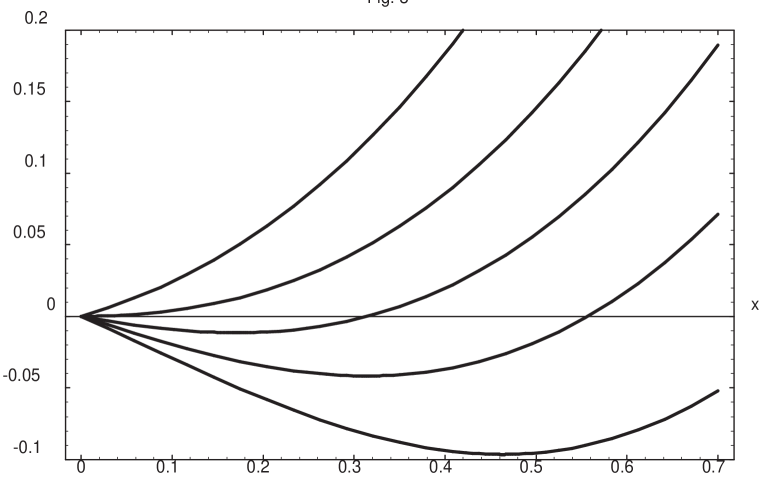
Figure 3: The curves, from left to right, represent the plots of $A_{1}(x,y)$ for $P=-1/2$ and $\sqrt{y}=1.95$, $2.13$, $2.3$, $2.5$ and $2.8$, respectively. (see Ref.[2]). The critical value $\sqrt{y}\approx 2.13$ corresponds to the second order transition.

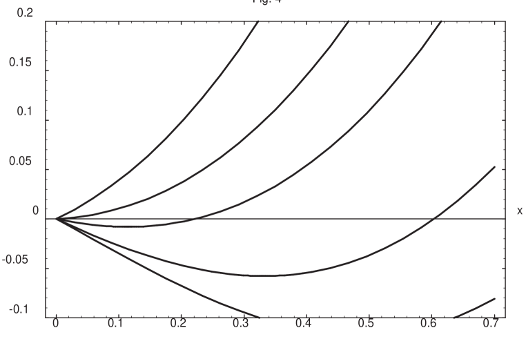
Figure 4: The curves, from left to right, shows the function $A_{2}(x,y)$ for $Q=6$ and $\sqrt{y}=.9$, $1$, $1.1$, $1.3$, $1.5$, respectively. The second order phase transition happens at $\sqrt{y}\approx 1$.

The typical behavior of the effective potentials in case of second order phase transitions is illustrated by Figures 3 and 4, which are obtained by using formulas (4.1) and (4.2). Figure 3 depicts the function $A_{1}(x,y)$ for $P=-1/2$ and Figure 4 gives $A_{2}(x,y)$ for $Q=6$. In both cases the critical radii $a_{c}$ and $\tilde{a}_{c}$ are in agreement with Eqs.(4.13) and (4.15).

4.3 Classification of models

As we have shown, the first order phase transitions always take place in the models of scalar electrodynamics (3.1) when constants $P$ and $Q$ are large and positive. On the other hand, if these constants are negative with large absolute values, the symmetry breaking corresponds to second order phase transitions.

An analytical study of the region of parameters $\xi$, $\lambda$ and $e^{2}$ (or $P_{cr}$ and $Q_{cr}$), where the kind of the phase transition changes from the first to the second order is difficult because the effective potentials have quite involved forms (4.1), (4.2). Thus, in principle, one should use here numerical methods. It is interesting, however, that the analytical estimates $P_{cr}=-\frac{1}{6}$ and $Q_{cr}={20\over 3}$ of Section 4.2 are in very good agreement with the numerical results. For dSI state this was first pointed out by Allen [2].

As we already mentioned, the symmetry breaking mechanism in the considered models is completely determined by the parameters $P$ and $Q$. By using their definitions (3.30), (3.32) one finds that

$$Q=4P+{8\pi^{2}\lambda\over 3e^{2}}+{32\over 3}~{}~{}~{}.$$ (4.18)

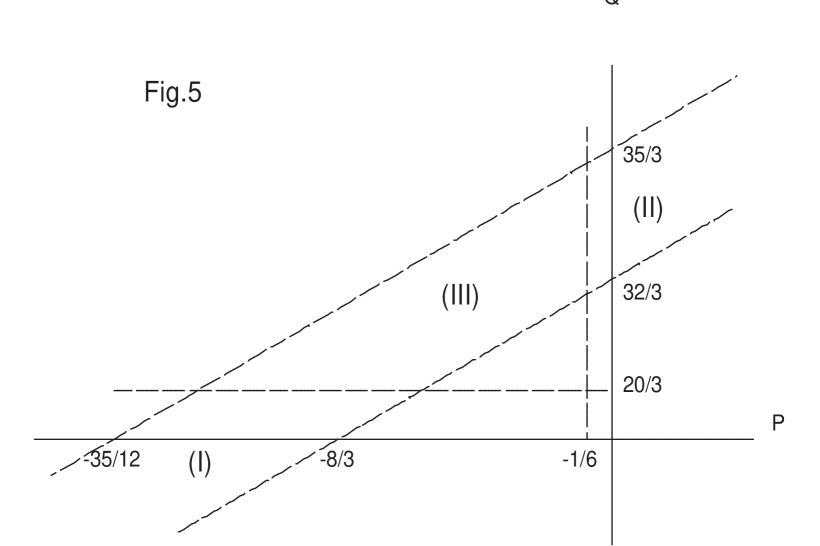
Figure 5: The regions (I), (II) and (III), bounded by dashed lines, represent the allowed areas in the $P$–$Q$ plane. If the parameters $P$ and $Q$ are chosen in regions (I) or (II), one has always second or first order phase transition, respectively, in both dSI and ZT states. In region (III) first order phase transitions take place in ZT state, whilst dSI state shows second order phase transitions.

Note that the parameter $\lambda$ must be chosen positive in order to have a scalar potential bounded from below. We also assumed that $\lambda\simeq e^{4}$ in order to have a considerable quantum correction to the classical potential coming from the gauge fields. For values $\lambda\gg e^{4}$ our perturbative approach is not reliable, so we have to restrict ourselves to the interval of parameters $0\leq\lambda e^{-2}\lower 3.01385pt\hbox{$\;\stackrel{{\scriptstyle\textstyle<}}{{\sim}}\;$}e^{2}$. Thus, by taking into account that $e^{2}/4\pi\simeq 10^{-2}$, we find with the help of Eq.(4.18) the allowed region in the $P$–$Q$ plane $0\leq Q-4P-32/3\lower 3.01385pt\hbox{$\;\stackrel{{\scriptstyle\textstyle<}}{{\sim}}\;$}1$. There we can make definite predictions about the properties of the considered models. This region is shown on Figure 5. It consists of three subregions (I), (II) and (III), bounded by dashed lines. Each subregion indicates a class of models with the same properties.
Region (I) is determined by inequalities $P<-1/6$ and $Q\leq 20/3$. If the coupling constants $\xi,e,\lambda$ satisfy these restrictions, the corresponding models undergo second order phase transitions in both dSI and ZT states.
In region (II) one has $P\geq-1/6$ and $Q>20/3$ and first order phase transitions in both dSI and ZT vacua.
Region (III) is the most interesting, since in this case $P<-1/6$ but $Q>20/3$, thus the system undergoes a first order phase transition in ZT case, whereas it has a second order phase transition in dSI case.

In case of minimal coupling ($\xi=0$), according to Eqs.(3.30) and (3.32), $P\leq-3/2<-1/6$ and $Q\leq 14/3<20/3$, and so only second order phase transitions are possible in both states.

5 Summary

We investigated the effective potential for the gauge models on the singular spherical domains $S^{4}_{\beta}$. The spectrum of the corresponding wave operators on these backgrounds can be found exactly and it enables one to calculate the potential with the help of the $\zeta$–function. We have shown that for arbitrary values of $\beta$ there is a simple relation (3.18) between the one-loop corrections to the potential from gauge and scalar fields. Thus in studying the gauge models in the de Sitter space one can make use of the computations of the scalar potential of Ref.[4]. The effective action on $S^{4}_{\beta}$ can be interpreted as the free energy of fields in static de Sitter space, where the parameter $\beta$ is the inverse temperature of the system. Thus, by changing $\beta$ one can learn how the presence of temperature affects the properties of such a quantum theory. The aim of the paper was to compare the phase structures of the gauge models in the de Sitter invariant vacuum, which is usually used in the quantum cosmology, with the structure of the normal vacuum which is the state at zero temperature.

According to our analysis both vacua have very similar properties in the extreme regimes of very small and very large curvatures. If the restoration of the gauge symmetry happens at large radius $a$ (small curvature) of the de Sitter space, then the corresponding phase transition is of first order regardless what vacuum is considered. Analogously, if the symmetry is restored at small values of $a$ (large curvature), one has second order phase transitions. The critical masses and radii are completely determined by the constants $P$ and $Q$, which are the functions of the parameters $\xi$, $e^{2}$ and $\lambda$. Expressions (4.11), (4.12) and (4.15) for the critical parameters in ZT state represent the new result.

We have also found the critical value $Q_{cr}=20/3$ for the parameter $Q$ , which separates models with second ($Q<20/3$) and first ($Q>20/3$) order phase transitions in ZT state. Finally we proved the existence of a class of the models ($P<-1/6$ and $Q>20/3$) where the kinds of phase transition in the two vacua are different.

The detailed analysis of the effective potential for all $\beta$’s is not given here, but it can be carried out in principle by making use of the properties of the $\zeta$–function. In the most interesting cases, however, it is sufficient to restrict the study to the expansions near the zero and Hawking temperatures, as it was done in Ref.[4].

Acknowledgements:  This work was supported in part by the Natural Sciences and Engineering Research Council of Canada.

Appendix A $\zeta$–function

Here we consider $\zeta$–function

$$\zeta^{(T)}\left(z\right)=\sum_{n=0}^{\infty}\sum_{l=1}^{\infty}D^{T}_{n}(\Lambda^{T}_{n,l})^{-z}+\sum_{n=1}^{\infty}\bar{D}^{T}_{n}(\Lambda^{T}_{n,0})^{-z}~{}~{}~{}$$ (A.1)

for the transverse operator in Eq.(3.12) which is defined for convenience in the dimensionless form as $a^{2}(\Delta^{T}_{\mu\nu}+g_{\mu\nu}e^{2}\varphi^{2})$.

According to [6] the degeneracies in four dimensions read

$$D^{T}_{n}=3(n+1)(n+2)~{}~{}~{},~{}~{}~{}\bar{D}^{T}_{n}=\frac{n}{2}(3n+5)~{}~{}~{},$$ (A.2)

while the eigen–values $\Lambda^{T}_{n,l}$ are

$$\Lambda^{T}_{n,l}=(n+\gamma l)(n+\gamma l+3)+2+e^{2}a^{2}\varphi^{2}~{}~{}~{},$$ (A.3)

where $\gamma=\beta_{H}/\beta$. As in Section 3, it is suitable to parametrize the function (A.1) by the parameters $\beta$ and $\sigma=\frac{1}{4}-e^{2}a^{2}\varphi^{2}$. Thus one can write

$$\zeta^{(T)}\left(z,\beta,\sigma\right)=\sum_{n=0}^{\infty}\sum_{l=1}^{\infty}D^{T}_{n}(\Lambda^{T}_{n,l}(\sigma))^{-z}+\sum_{n=1}^{\infty}\bar{D}^{T}_{n}(\Lambda^{T}_{n,0}(\sigma))^{-z}~{}~{}~{},$$ (A.4)

where

$$\Lambda^{T}_{n,l}(\sigma)=(n+\gamma l+3/2)^{2}-\sigma~{}~{}~{}.$$ (A.5)

Function (A.4) has an interesting relation to the $\zeta$–function of the scalar Laplace operator $-a^{2}\nabla^{\mu}\nabla_{\mu}+9/4-\sigma$ on the same spherical domain $S^{4}_{\beta}$. These operators were studied in [4], where they were shown to possess the eigenvalues coinciding with (A.5). So the scalar $\zeta$–function is represented in the form

$$\zeta^{(0)}(z,\beta,\sigma)=\sum_{n=0}^{\infty}\sum_{l=1}^{\infty}D^{(0)}_{n}(\Lambda^{T}_{n,l}(\sigma))^{-z}+\sum_{n=1}^{\infty}\bar{D}^{(0)}_{n}(\Lambda^{T}_{n,0}(\sigma))^{-z}~{}~{}~{},$$ (A.6)

where the degeneracies

$$D^{(0)}_{n}=(n+1)(n+2)~{}~{}~{},~{}~{}~{}\bar{D}^{(0)}_{n}=\frac{1}{2}(n+1)(n+2)~{}~{}~{}$$ (A.7)

differ from the degeneracies (A.2) of the vector operator. By comparing Eqs. (A.6) and (A.7) with (A.4) and (A.2) one obtains

$$\zeta^{(T)}\left(z,\beta,\sigma\right)=3\zeta^{(0)}(z,\beta,\sigma)-2\sum_{n=0}^{\infty}\left(n+\frac{3}{2}\right)\left[\left(n+\frac{3}{2}\right)^{2}-\sigma\right]^{-z}=$$

$$3\zeta^{(0)}(z,\beta,\sigma)-2\sum_{k=0}^{\infty}\sigma^{k}C_{k}(z)\zeta_{R}\left(2z+2k-1,{3\over 2}\right)~{}~{}~{},$$ (A.8)

where $C_{k}(z)=\Gamma(z+k)/(k!\Gamma(z))$. To get the second equality of this equation one has to decompose the last term in $\sigma$ and make use of the definition of the Riemann zeta–function $\zeta_{R}(z,a)$. The function $\zeta^{(0)}(z,\beta,\sigma)$ has been studied in detail in the previous works [2, 4], and this makes the analysis of $\zeta^{(T)}(z,\beta,\sigma)$ much more easy. In particular, by taking into account the result of [4] and Eq.(A.8) one obtains

$$\zeta^{(T)}\left(0,\beta,\sigma\right)=3\zeta^{(0)}\left(0,\beta,\sigma\right)+{11\over 12}-\sigma=$$

$${3\over\gamma}\left[{51-60{\gamma^{2}}-8\gamma^{4}\over 2880}+{2\gamma^{2}-3\over 24}\sigma+{\sigma^{2}\over 12}\right]+{11\over 12}-\sigma~{}~{}~{}.$$ (A.9)

However, the analysis of the derivative of the generalized $\zeta$–function

$${d\over dz}\zeta^{(T)}\left(0,\beta,\sigma\right)=3{d\over dz}\zeta^{(0)}\left(0,\beta,\sigma\right)$$

$$-2\left[2\zeta^{\prime}_{R}\left(-1,{3\over 2}\right)-\sigma\psi\left({3\over 2}\right)+\sum_{k=2}^{\infty}{\sigma^{k}\over k}\zeta_{R}\left(2k-1,{3\over 2}\right)\right]$$ (A.10)

is more involved and we consider only two of the most interesting cases where the result can be obtained in the simple analytical form.

– Temperatures close to the Hawking temperature –

This case was investigated by B. Allen in Ref.[2] and our aim here is to rederive his result for ${d\over dz}\zeta^{(0)}\left(0,\beta_{H},\sigma\right)$ in a different way with the help of Eq.(A.8). For the scalar $\zeta$–function one can find the following representation [2]

$${d\over dz}\zeta^{(0)}\left(0,\beta_{H},\sigma\right)=-\frac{1}{3}\left(\int_{{1\over 2}}^{{1\over 2}+\sqrt{\sigma}}+\int_{{1\over 2}}^{{1\over 2}-\sqrt{\sigma}}\right)u\left(u-{1\over 2}\right)(u-1)\psi(u)du+{\sigma^{2}\over 12}+{\sigma\over 72}$$

$$+\frac{2}{3}\left[\zeta_{R}^{\prime}\left(-3,\frac{3}{2}\right)-\frac{1}{4}\zeta_{R}^{\prime}\left(-1,\frac{3}{2}\right)\right]~{}~{}~{},$$ (A.11)

where $\psi(u)\equiv\Gamma^{\prime}(u)/\Gamma(u)$. By using relation $\zeta_{R}(n+1,z)=(-1)^{n+1}{d^{n}\over dz^{n}}\psi(z)/n!$ it is possible to show that

$$-\sigma\psi\left({3\over 2}\right)+\sum_{k=1}^{\infty}{\sigma^{k+1}\over k+1}\zeta_{R}\left(2k+1,\frac{3}{2}\right)=\left(\int_{{3\over 2}}^{{3\over 2}+\sqrt{\sigma}}+\int_{{3\over 2}}^{{3\over 2}-\sqrt{\sigma}}\right)\left({3\over 2}-u\right)\psi(u)du~{}~{}~{}.$$ (A.12)

Thus by substituting Eqs.(A.11) and (A.12) into (A.8) and using the properties of the $\psi$–function one gets

$${d\over dz}\zeta^{(T)}\left(0,\beta,\sigma\right)=-\left(\int_{{3\over 2}}^{{3\over 2}+\sqrt{\sigma}}+\int_{{3\over 2}}^{{3\over 2}-\sqrt{\sigma}}\right)u\left(u-{3\over 2}\right)(u-3)\psi(u)du+\frac{\sigma^{2}}{4}-\frac{11}{24}\sigma$$

$$+2\zeta_{R}^{\prime}\left(-3,\frac{3}{2}\right)-\frac{9}{2}\zeta_{R}^{\prime}\left(-1,\frac{3}{2}\right)-3\left({\beta\over\beta_{H}}-1\right)\left[\frac{41}{144}\sigma-\frac{\sigma^{2}}{8}-\frac{973}{5760}\right.$$

$$\left.+\frac{1}{192}\left(16{\sigma}^{2}-40\sigma+9\right)\left(\psi\left(\frac{3}{2}+\sqrt{\sigma}\right)+\psi\left(\frac{3}{2}-\sqrt{\sigma}\right)\right)\right]+O\left((\beta-\beta_{H})^{2}\right)~{}~{}~{}.$$ (A.13)

As one can see, this expression coincides at $\beta=\beta_{H}$ with the result reported in Ref.[2].

– Vanishing temperature –

To derive $d\zeta^{(T)}/dz$ in the zero temperature limit one can use the method suggested in [4]. Unfortunately, the final formula given in [4] has a wrong form because of a misprint, so here we use the opportunity to represent the correct answer. According to relation (A.8) and Eq.(B2) of Ref.[4], one has

$$\beta_{H}\lim_{\beta\rightarrow\infty}\left(\beta^{-1}{d\over dz}\zeta^{(T)}\left(0,\beta,\sigma\right)\right)=3\beta_{H}\lim_{\beta\rightarrow\infty}\left(\beta^{-1}{d\over dz}\zeta^{(0)}\left(0,\beta,\sigma\right)\right)$$

$$=3\sum_{k=0}^{\infty}C_{k}(z){(\sqrt{\sigma})^{2k}\over 2z+2k-1}\left[\zeta_{R}(2z+2k-3,3/2)-\frac{1}{4}\zeta_{R}(2z+2k-1,3/2)\right]\equiv 3f(z,\sigma)~{}~{}~{}.$$ (A.14)

The function $f(z,\sigma)$ was introduced in [4], where it was shown to be related to $\zeta^{(0)}\left(z,\beta_{H},\sigma\right)$, see (A.11), by the differential equation

$${d\over d\sqrt{\sigma}}\left[f(z,\sigma)(\sqrt{\sigma})^{2z-1}\right]=3\sigma^{z-1}\zeta^{(0)}\left(0,\beta_{H},\sigma\right)~{}~{}~{}.$$ (A.15)

Thus, one can write

$${d\over dz}f(0,\sigma)=\sqrt{\sigma}\int_{0}^{\sqrt{\sigma}}{dy\over y^{2}}\left[3\left({d\over dz}\zeta^{(0)}\left(0,\beta_{H},y^{2}\right)-{d\over dz}\zeta^{(0)}\left(0,\beta_{H},0\right)\right)-2(f(0,y^{2})-f(0,0))\right]$$

$$-\left(3{d\over dz}\zeta^{(0)}\left(0,\beta_{H},0\right)-2f(0,0)\right)~{}~{}~{}.$$ (A.16)

By making use of (A.11) in (A.16) one finally finds

$$\beta_{H}\lim_{\beta\rightarrow\infty}\left(\beta^{-1}{d\over dz}\zeta^{(T)}\left(0,\beta,\sigma\right)\right)=$$

$$3\left(\int_{\frac{1}{2}}^{\frac{1}{2}+\sqrt{\sigma}}+\int_{\frac{1}{2}}^{\frac{1}{2}-\sqrt{\sigma}}\right)u\left(u-\frac{1}{2}\right)(u-1)\psi(u)du-3\sqrt{\sigma}\left(\int_{\frac{1}{2}}^{\frac{1}{2}+\sqrt{\sigma}}-\int_{\frac{1}{2}}^{\frac{1}{2}-\sqrt{\sigma}}\right)u(u-1)\psi(u)du$$

$$+{1\over 12}\sigma^{2}+{7\over 8}\sigma+{17\over 160}-6\zeta_{R}^{\prime}\left(-3,\frac{3}{2}\right)+\frac{3}{2}\zeta_{R}^{\prime}\left(-1,\frac{3}{2}\right)~{}~{}~{}.$$ (A.17)

References

- [1] G.M. Shore, Ann. Phys. 128 (1980) 376.
- [2] B. Allen, Nucl. Phys. B226 (1983) 228.
- [3] B. Allen, Ann. Phys. 161 (1985) 152.
- [4] D.V. Fursaev and G. Miele, Phys. Rev. 49 (1994) 987.
- [5] A.D.Linde, Particle Physics and Inflationary Cosmology (Harwood Academic Publishers, New York 1990).
- [6] L. De Nardo, D.V. Fursaev and G. Miele, Heat-kernel coefficients and spectra of the vector Laplacians on spherical domains with conical singularities, hep-th/9610011, to appear in Class. Quantum Gravity.
- [7] G.W. Gibbons and S.W. Hawking, Phys. Rev. D15 (1977) 2738.
- [8] G.W. Gibbons and S.W. Hawking, Phys. Rev. D15 (1977) 2752.
- [9] F. Buccella, G. Esposito and G .Miele, Class. Quantum Grav. 9 (1992) 1499.
- [10] G. Esposito, G. Miele and L. Rosa, Class. Quantum Grav. 11 (1994) 2031.
- [11] J.B. Hartle and S.W. Hawking, Phys. Rev. D13 (1976) 2188.
- [12] D.G. Boulware, Phys. Rev. 11 (1975) 1401; ibid 12 (1975) 350.
- [13] E.A. Tagirov, Ann. Phys., NY 76 (1973) 561.
- [14] P. Candelas and D. Raine, Phys. Rev. D12 (1975) 965.
- [15] J.S. Dowker and R. Critchley, Phys. Rev. D13 (1976) 224.
- [16] J.S. Dowker, Phys. Rev. 18 (1978) 1856.
- [17] J.S. Dowker, J. Phys. A10 (1977) 115.
- [18] S.P. deAlvis and N. Ohta, Phys. Rev. D52 (1995) 3529.
- [19] J.-G. Demers, R. Lafrance and R.C. Myers, Phys. Rev. D52 (1995) 2245.
- [20] S.N. Solodukhin, Phys. Rev. D53 (1996) 824.
- [21] V.P. Frolov, D.V. Fursaev and A.I. Zelnikov, Nucl. Phys. B486 (1997) 339.
- [22] B.S.Kay and R.M.Wald, Phys. Rep. 207(2) (1991) 49.
- [23] D.V. Fursaev and G. Miele, Class. Quantum Grav. 12 (1995) 393.
- [24] S. Coleman and E. Weinberg, Phys. Rev. D7 (1973) 1888.
- [25] S.W. Hawking, Commun. Math. Phys 55 (1977) 133.
- [26] G. Cognola, K. Kirsten and L. Vanzo, Phys. Rev. D49 (1994) 1029.
- [27] D.V. Fursaev, Phys. Lett. B334 (1994) 53.
- [28] L. Susskind and J. Uglum, Phys. Rev. D50 (1994) 2700.
- [29] S.N. Solodukhin, Phys. Rev. D51 (1995) 609.
- [30] D.V. Fursaev, Mod. Phys. Lett. A10 (1995) 649.
- [31] D.V. Fursaev and S.N. Solodukhin, Phys. Lett. B365 (1996) 51.
- [32] D. Kabat, Nucl. Phys. B453 (1995) 281.
- [33] D.V. Fursaev and G. Miele, Nucl. Phys. B484 (1997) 697.
- [34] N.D. Birrell and P.C.W. Davies, Quantum Fields in Curved Space, Cambridge University Press, Cambridge 1982.
- [35] M. Abramowitz and I.A. Stegun, Handbook of mathematical functions (Dover publications, inc., New York).