Imperial/TP/96-97/38

hep-th/9703118

BPS bound states, supermembranes,

and T-duality in M-theory

Jorge G. Russo

Theoretical Physics Group, Blackett Laboratory

Imperial College, London SW7 2BZ, U.K.

jrusso@ic.ac.uk

Abstract

This is an introductory review on the eleven-dimensional description of the BPS bound states of type II superstring theories, and on the role of supermembranes in M-theory. The first part describes classical solutions of 11d supergravity which upon dimensional reduction and T-dualities give bound states of NS-NS and R-R $p$-branes of type IIA and IIB string theories. In some cases (e.g. $(q_{1},q_{2})$ string bound states of type IIB string theory), these non-perturbative objects admit a simple eleven-dimensional description in terms of a fundamental 2-brane. The BPS excitations of such 2-brane are calculated and shown to exactly match the mass spectrum for the BPS $(q_{1},q_{2})$ string bound states. Different 11d representations of the same bound state can be used to provide inequivalent (T-dual) descriptions of the oscillating BPS states. This permits to test T-duality beyond perturbation theory and, in certain cases, to evade membrane instabilities by going to a stable T-dual representation. We finally summarize the results indicating in what regions of the modular parameter space a supermembrane description for M-theory on ${\bf R^{9}}\times{\bf T^{2}}$ seems to be adequate.

1 Introduction

In type II superstring theories, classical solutions representing solitons can be classified into two types: the NS-NS and the R-R solitons, according to whether they carry charge of gauge fields originating from the NS-NS or R-R sector of the theory (for recent reviews and references see [1]-[6]). In certain cases, these solitons can form bound states [7, 8, 2] and the corresponding classical solution preserves some of the original supersymmetries. These are the BPS bound states. The bound states can be marginal (or at threshold), meaning that they have zero binding energies (typically, $M_{1+2}=M_{1}+M_{2}$), or else non-marginal (or non-threshold), with a finite binding energy (viz. $M_{1+2}=\sqrt{M_{1}^{2}+M_{2}^{2}}$ ). In this paper we will focus on these last ones [9] (different studies of supersymmetric M-brane solutions can be found e.g. in refs.  [10]-[16]).

Type IIB superstring theory can be connected to M theory by the sequence

$${\rm Type\ IIB\ on\ }S^{1}\ \smash{\mathop{\longrightarrow}\limits_{T}}\ {\rm Type\ IIA\ on\ }S^{1}\ \smash{\mathop{\longrightarrow}\limits_{\rm R_{1}\to\infty}}\ {\rm 10d\ Type\ IIA}\smash{\mathop{\longrightarrow}\limits_{g^{2}\to\infty}}\ {\rm M\ theory}$$ (1)

In the presence of several isometries, the path from eleven dimensions to type IIB string theory is not unique. The same classical solution of eleven-dimensional supergravity can be used to obtain different solutions of type IIA superstring theory, according to the direction we reduce. Furthermore, if there is an extra isometry, the T-duality transformation connecting type IIA and type IIB theory can be done in a direction which is either perpendicular or parallel to the brane. There are many possible paths which are not manifest in this sequence and, as a result, there are inequivalent eleven-dimensional representations of the same type IIB solutions.

The equations of motion of type IIB superstring theory are symmetric under the action of $SL(2,{\bf R})$ transformations [17, 18]. Starting with the fundamental NS-NS string solution in type IIB superstring theory, by an $SL(2,{\bf R})$ transformation one can obtain a general solution which represents the bound state of NS-NS and R-R strings. From the viewpoint of eleven dimensions, such transformation simply corresponds to a reparametrization; the $SL(2,{\bf R})$ transformations are viewed as the modular transformations of the target torus [7, 19]. This illustrates a characteristic of M-theory: in a number of cases, what is non-perturbative from string theory viewpoint can be described in eleven dimensions within the domain of perturbation theory. Many complicated-looking solutions of string theory take a remarkably simple form when lifted to eleven dimensions. This is because the 11d counterpart of performing a U-duality transformation and adding Kaluza-Klein charges to a NS-NS soliton does not further complicate the solution; it gives the same solution in terms of some rotated coordinates or with a momentum boost. In particular, as we shall discuss, the string bound states admit an exact description in terms of a fundamental 2-brane with a certain charge and a momentum boost.

In the next section, we will discuss the eleven dimensional origin of different non-marginal BPS configurations of type II string theories as classical solutions of the supergravity effective field theory in eleven dimensions. Following [9, 20], we will explicitly construct the solutions which upon reduction and dualities give different $p$-brane bound states (other interesting discussions on non-marginal bound states in type II theories can be found in refs. [21, 22]). In lower dimensions, these can be obtained from pure NS-NS configurations by U-duality transformations (i.e. combining $O(d,d)$ and $SL(2,{\bf R})$ transformations).

In section 3 the connection between type IIA superstrings and supermembranes wrapped on ${\bf R}^{10}\times S^{1}$ will be investigated by using the light-cone Hamiltonian approach. The question that will be addressed (investigated in [23]) is whether at small compactification radius the only light excitations are those contained in the type IIA superstring spectrum. It turns out that this is not the case, and there are extra quantum states, which do not decouple in the zero radius limit. We shall return to this point in sect. 4, where it will be argued that standard supermembrane theory is not suitable in certain regimes.

Given that the string-string bound states correspond to fundamental 2-branes in eleven dimensions, it is of interest to determine the spectrum of oscillations of these 2-branes. This can be done by using the light-cone Hamiltonian approach of supermembrane theory. Although this is a non-linear theory, it will be shown that it is exactly solvable in a certain limit [9]. In the BPS sector, a remarkable correspondence with the bound state spectrum proposed by Schwarz [7] will be found. We will also calculate the spectrum for another (T-dual) representation of the same string-string bound state [20], and find that in the BPS sector the spectra corresponding to the T-dual backgrounds match, which may be regarded as a test of T-duality beyond perturbation theory (since the matching holds true for BPS quantum states of masses $\alpha^{\prime}M^{2}=O(1/g^{2})$). Some surprises arise in the non-BPS sector: the assumption of exact T-duality in M-theory implies that supermembrane theory can only be an adequate description in some corners of the modular parameters. Possible corrections to the membrane Hamiltonian outside these corners can be deduced by using the T-dual representation.

2 Eleven-dimensional origin of BPS bound states

We will now map 10d supergravity solutions of type IIA and IIB into 11d supergravity. The notation will be as follows:

Type IIB supergravity multiplet:

$$NS\otimes NS:\ \ \ \{\phi_{B},\ B^{(1)}_{\mu\nu},\ g_{\mu\nu}\}$$

$$R\otimes R:\ \ \ \{\chi,\ B^{(2)}_{\mu\nu},\ D_{\mu\nu\rho\sigma}\}$$

Type IIA supergravity multiplet:

$$NS\otimes NS:\ \ \ \{\phi_{A},\ B_{\mu\nu},\ \tilde{g}_{\mu\nu}\}$$

$$R\otimes R:\ \ \ \{A_{\mu},\ A_{\mu\nu\rho}\}$$

$d=11$ supergravity multiplet

$$\{g^{(11)}_{\hat{\mu}\hat{\nu}},\ C_{\hat{\mu}\hat{\nu}\hat{\rho}}\}\$$

Type IIA and 11d supergravity solutions are connected by dimensional reduction:

$$ds^{2}_{11}=g^{(11)}_{\hat{\mu}\hat{\nu}}dx^{\hat{\mu}}dx^{\hat{\nu}}=e^{-2\phi_{A}/3}\tilde{g}_{\mu\nu}dx^{\mu}dx^{\nu}+e^{4\phi_{A}/3}(dy-A_{\mu}dx^{\mu})^{2}\ ,$$

$$A_{\mu\nu\rho}=C_{\mu\nu\rho}\ ,\ \ \ \ B_{\mu\nu}=C_{\mu\nu y}\ .$$ (2)

The T-duality map between type IIA/IIB solutions is given by [24]

$$\tilde{g}_{yy}=g_{yy}^{-1}\ ,\ \ \ \ e^{2\phi_{A}}={e^{2\phi_{B}}\over g_{yy}}\ ,$$

$$\tilde{g}_{\mu\nu}=g_{\mu\nu}-g_{yy}^{-1}\big{(}g_{y\mu}g_{y\nu}-B_{y\mu}^{(1)}B_{y\nu}^{(1)}\big{)}\ ,\ \ \ \ \tilde{g}_{y\mu}={B_{y\mu}^{(1)}\over g_{yy}}\ \ ,$$

$$A_{y\mu\nu}={2\over 3}\big{[}B_{\mu\nu}^{(2)}+2g_{yy}^{-1}B_{y[\mu}^{(2)}g_{\nu]y}\big{]}\ ,\ \$$

$$A_{\mu\nu\rho}={8\over 3}D_{y\mu\nu\rho}+\epsilon^{ij}B_{y[\mu}^{(i)}B_{\nu\rho]}^{(j)}+g_{yy}^{-1}\epsilon^{ij}B_{y[\mu}^{(i)}B_{y\nu}^{(j)}g_{\rho]y}\ ,$$

$$B_{\mu\nu}=B_{\mu\nu}^{(1)}+2g_{yy}^{-1}B_{y[\mu}^{(1)}g_{\nu]y}\ ,\ \ \ \ B_{y\mu}={g_{y\mu}\over g_{yy}}\ ,$$

$$A_{\mu}=-B_{y\mu}^{(2)}+\chi B_{y\mu}^{(1)}\ \ ,\ \ \ \ \ A_{y}=\chi\ .$$ (3)

Let us now consider type IIB superstring theory on ${\bf R^{9}}\times S^{1}$, and let $y_{1}$ be the coordinate of $S^{1}$ with radius $R_{1}^{\prime}$. The basic object that will be used as starting point is the fundamental string solution [25], which in the string frame is given by

$$ds^{2}_{10B}=\tilde{H}_{2}^{-1}\big{(}-dt^{2}+dy_{1}^{2}\big{)}+dx_{i}dx_{i}\ ,\ \ \ \ e^{2\phi}=\tilde{H}_{2}^{-1}\ ,$$

$$B_{ty_{1}}^{(1)}=-\tilde{H}_{2}^{-1}(\tilde{H}_{2}-1)\ ,\ \ \ \ B_{ty_{1}}^{(2)}=0\ ,$$

$$\tilde{H}_{2}=1+{\tilde{Q}\over r^{6}}\ ,\ \ \ \ r^{2}=x_{i}x_{i}\ .$$ (4)

[Throughout indices $i$ will run over all remaining directions.] By a straightforward application of the IIA/B T-duality map (3), one finds the type IIA background that is obtained by a T-duality transformation in $y_{1}$ [26, 27]:

$$ds^{2}_{10A}=-dt^{2}+dy_{1}^{2}+(\tilde{H}_{2}-1)(dt+dy_{1})^{2}+dx_{i}dx_{i}\ ,\$$

$$e^{2\phi_{A}}=1\ ,\ \ \ A_{\mu}=A_{\mu\nu\rho}=B_{\mu\nu}=0\ ,$$ (5)

representing a gravitational wave moving along $y_{1}$. In the string theory, for T-duality to be a symmetry, $y_{1}$ must have periodicity $R_{1}=\alpha^{\prime}/R_{1}^{\prime}$.

Using eq. (2), we now lift this solution to $d=11$, obtaining

$$ds^{2}_{11}=-dt^{2}+dy_{1}^{2}+dy_{2}^{2}+(\tilde{H}_{2}-1)(dt+dy_{1})^{2}+dx_{i}dx_{i}\ ,\$$

$$C_{\mu\nu\rho}=0\ ,$$ (6)

again representing a gravitational wave. Note that, since $y_{1}$ is periodic, the momentum $\tilde{Q}$ must be quantized in units of $1/R_{1}$, which with the correct normalization gives

$$\tilde{Q}=c_{0}{n\over R_{1}}\ ,\ \ \ \ c_{0}={\kappa_{9}^{2}\over 3\omega_{7}}\ ,\ \ \ \ \kappa_{9}^{2}=2\pi R_{1}\kappa_{10}^{2}\ ,\ \ \ \omega_{7}={\pi^{4}\over 3}\ .$$

From ten-dimensional viewpoint, this quantization condition arises as the Dirac quantization implied by the existence of the five brane.

The solution (6) preserves half of the supersymmetries, and it admits a simple generalization where $\tilde{H}_{2}-1\equiv W$ is replaced by $W=W(u,x^{i})$, with $\partial^{2}_{x}W=0$ [27]. A solution of interest is $W=f_{i}(u)x^{i}$, representing right-moving waves in the direction of the boost. For a solution carrying momentum along a given direction, supersymmetry is preserved by adding waves moving in the direction of the momentum [27, 28].

In [7], the $(q_{1},q_{2})$ string bound states were obtained by applying an $SL(2,{\bf Z})$ transformation to the fundamental string solution. The corresponding transformation in $d=11$ turns out to be quite simple: take the solution (6) and make a rotation in $y_{1},y_{2}$ plane. This gives

$$ds^{2}_{11}=-dt^{2}+dy_{1}^{2}+dy_{2}^{2}+(\tilde{H}_{2}-1)(dt-\cos\theta dy_{1}-\sin\theta dy_{2})^{2}+dx_{i}dx_{i}\ ,\$$

$$W={\tilde{Q}_{q}\over r^{6}}\ ,\ \ \ \tilde{Q}_{q}=c_{0}\sqrt{{l_{1}^{2}\over R_{1}^{2}}+{l_{2}^{2}\over R_{2}^{2}}}=\tilde{Q}\sqrt{q_{1}^{2}+q_{2}^{2}\tau_{2}^{2}}\ ,\ \$$ (7)

$$\cos\theta={q_{1}\over\sqrt{q_{1}^{2}+q_{2}^{2}\tau_{2}^{2}}}\ ,\ \ \ \ \tau_{2}={R_{1}\over R_{2}}=e^{-\phi_{B0}}\ .$$ (8)

Here $l_{1},l_{2}$ are integer numbers corresponding to the Kaluza-Klein momenta in $y_{1},y_{2}$ directions, and we have introduced the relatively prime integers $q_{1},q_{2}$ by $(l_{1},l_{2})=n(q_{1},q_{2})$. Upon reduction we now find

$$ds^{2}_{10A}=K^{1/2}\big{[}-K^{-1}d\tilde{t}^{2}+d\tilde{y}_{1}^{2}+dx_{i}dx_{i}\big{]}\ ,\ \ \ \$$

$$e^{4\phi/3}=K\ ,\ \ \ \ K=1+\sin^{2}\theta\ W\ ,$$

$$\tilde{t}={1\over\sin\theta}\big{(}t-\cos\theta y_{1}\big{)}\ ,\ \ \ \ \tilde{y}_{1}={1\over\sin\theta}\big{(}y_{1}-\cos\theta t\big{)}\ .$$ (9)

This represents a 0-brane with a finite boost with velocity $v=\cos\theta$ [9]. By T-duality along $y_{1}$, we find the corresponding type IIB solution

$$ds^{2}_{10B}=K^{1/2}\big{[}\tilde{H}_{2}^{-1}\big{(}-dt^{2}+dy_{1}^{2}\big{)}+dx_{i}dx_{i}\big{]}\ ,$$

$$e^{2\phi}=\tilde{H}_{2}^{-1}K^{2}\ ,\ \ \ \ \chi=\sin\theta\cos\theta WK^{-1}\ ,$$

$$B_{ty_{1}}^{(1)}=-\cos\theta W\tilde{H}_{2}^{-1}\ ,\ \ \ \ B_{ty_{1}}^{(2)}=-\sin\theta W\tilde{H}_{2}^{-1}\ .$$ (10)

For $\cos\theta=0$, one has $K=1$ and the solution reduces to the fundamental string solution (or $1_{NS}$); for $\cos\theta=1$, one has $K=\tilde{H}_{2}$ and the solution represents the R-R string (or $1_{R}$). Schematically, we have obtained the sequence

$$\nearrow\ \smash{\mathop{\longrightarrow}\limits_{\rm red}}\ 0_{R}\uparrow\ \smash{\mathop{\longrightarrow}\limits_{T_{y_{1}}}}\ 1_{R}+1_{NS}$$ (11)

Another basic object in eleven dimensions is the 2-brane given by [29]

$$ds^{2}_{11}=H_{2}^{-2/3}\big{[}-dt^{2}+dy_{1}^{2}+dy_{2}^{2}\big{]}+H_{2}^{1/3}dx_{i}dx_{i}\ ,$$

$$C_{3}=H_{2}^{-1}dt\wedge dy_{1}\wedge dy_{2}\ ,\ \ \ \ H_{2}=1+{Q\over r^{6}}\ ,$$ (12)

where $Q=c_{0}{w_{0}R_{1}\over\alpha^{\prime}}$, and $w_{0}$ represents the winding number of the 2-brane around the target torus $y_{1},y_{2}$. Upon reduction, this gives

$$ds^{2}_{10A}=H_{2}^{-1}\big{[}-dt^{2}+dy_{1}^{2}\big{]}+dx_{i}dx_{i}\ ,$$

$$e^{2\phi}=H_{2}^{-1}\ ,\ \ \ B_{y_{1}t}=C_{y_{2}y_{1}t}=H_{2}^{-1}\ ,$$ (13)

i.e., the fundamental string solution in type IIA superstring theory. After $T_{y_{1}}$-duality, we get a plane wave in type IIB. Summarizing:

$$2\ \smash{\mathop{\longrightarrow}\limits_{\rm red}}\ 1_{NS}\ \smash{\mathop{\longrightarrow}\limits_{T_{y_{1}}}}\ \uparrow$$ (14)

Combining with the previous result (11), we now start with the $2\nearrow$ background given by [9]

$$ds^{2}_{11}=H_{2}^{-2/3}\big{[}-dt^{2}+dy_{1}^{2}+dy_{2}^{2}+(\tilde{H}_{2}-1)(dt-dz_{1})^{2}\big{]}+H_{2}^{1/3}dx_{i}dx_{i}\ ,\$$

$$C_{3}=H_{2}^{-1}dt\wedge dy_{1}\wedge dy_{2}\ ,\ \ \ \ z_{1}=y_{1}\cos\theta+y_{2}\sin\theta\ ,$$ (15)

and get

$$2\nearrow\ \smash{\mathop{\longrightarrow}\limits_{\rm red}}\ 1_{NS}+0_{R}+\uparrow\ \smash{\mathop{\longrightarrow}\limits_{T_{y_{1}}}}\ \uparrow+1_{R}+1_{NS}$$ (16)

The final solution in type IIB superstring theory represents the 1/4 supersymmetric $(q_{1},q_{2})$ string bound state with a boost along $y_{1}$ direction, with the metric

$$ds^{2}_{10B}=K^{1/2}\big{[}\tilde{H}_{2}^{-1}\big{(}-dt^{2}+dy_{1}^{2}+(H_{2}-1)(dt-dy_{1})^{2}\big{)}+dx_{i}dx_{i}\big{]}\ ,$$ (17)

and all other fields as in eq. (10).

The fundamental string background (4) solves the equations of motion at $r\neq 0$. In order to solve the equations of motion at $r=0$, a string-like source term needs to be added [25], with tension

$$T={\omega_{7}\over\kappa^{2}_{10}}\tilde{Q}\ .$$

For the $(q_{1},q_{2})$ string background, the relevant string source must have tension

$$T_{q}={\omega_{7}\over\kappa^{2}_{10}}\tilde{Q}_{q}=T\sqrt{q_{1}^{2}+q_{2}^{2}\tau_{2}^{2}}\ .\$$

This has led Schwarz to propose that, at weak coupling, the spectrum of oscillations of the $(q_{1},q_{2})$ string bound state must be given by the usual free string spectrum, with $T\to T_{q}$. The mass formula is then

$$M^{2}_{\rm IIB} ={w_{0}^{2}\over{R^{\prime}_{1}}^{2}}+4\pi^{2}T^{2}_{q}n^{2}{R^{\prime}_{1}}^{2}+4\pi T_{q}(N_{R}+N_{L})$$ (18)

$$={l_{1}^{2}{R_{1}^{\prime}}^{2}\over{\alpha^{\prime}}^{2}}+{w_{0}^{2}\over{R_{1}^{\prime}}^{2}}+{l_{2}^{2}\over R_{2}^{2}}+{4\pi T\over n}\sqrt{l_{1}^{2}+l_{2}^{2}e^{-2\phi_{0}}}(N_{R}+N_{L})\ ,$$

$$N_{R}-N_{L}=w_{0}n\ .\$$

The zero mode part of this formula (which already contains information about the non-trivial tension) is in exact correspondence with the mass formula of a wrapped supermembrane [7] . To see this, we first perform a T-duality transformation and get

$$M^{2}_{\rm IIA}={l_{1}^{2}\over R_{1}^{2}}+{l_{2}^{2}\over R_{2}^{2}}+{w_{0}^{2}{R_{1}}^{2}\over{\alpha^{\prime}}^{2}}+{4\pi T\over n}\sqrt{l_{1}^{2}+l_{2}^{2}e^{-2\phi_{0}}}(N_{R}+N_{L})\ .$$

For a wrapped membrane, we have

$$M^{2}=(w_{0}AT_{3})^{2}+{l_{1}^{2}\over R_{1}^{2}}+{l_{2}^{2}\over R_{2}^{2}}+...\ ,$$

where $w_{0},~{}A,~{}T_{3}$ are the membrane winding number, area and tension respectively, and dots represent the oscillator contributions that we are for the moment ignoring. By writting

$$w_{0}AT_{3}=4\pi^{2}w_{0}R_{1}R_{2}T_{3}=2\pi R_{1}w_{0}T\ ,\ \ \ \ T\equiv 2\pi R_{2}T_{3}\ ,$$

and identifying $T$ with the string tension, we see that the zero mode part of the membrane mass formula agrees with the string bound state counterpart.

The mass formula (18) should be exact for BPS states. In particular, it should not receive additional corrections as the type IIA string coupling $g^{2}=R_{2}^{2}/\alpha^{\prime}$ is varied from $0$ (where eq. (18) applies) to $\infty$. In the BPS sector, it is meaningful to compare the spectrum (18) with the BPS excitations of the 2-brane. For generic BPS states, $N_{R}=w_{0}n\neq 0$; the oscillator contribution is indeed non-vanishing and we must calculate it in order to establish the equivalence between mass formulas [9]. This will be done in section 4.

Starting with the $(q_{1},q_{2})$ string bound state with an extra isometry in the coordinate $y_{3}$, we can apply $T_{y_{3}}$ duality and then lift the resulting solution to eleven dimensions, obtaining an alternative 11d representation of the type IIB string-string bound state. Schematically

$$1_{NS}+1_{R}+\uparrow\ \smash{\mathop{\longrightarrow}\limits_{T_{y_{3}}}}\ 1_{NS}+2_{R}+\uparrow\ \smash{\mathop{\longrightarrow}\limits_{\rm lift}}\ 2\uparrow$$

One obtains [20]

$$ds^{2}_{11}=\tilde{H}_{2}^{-2/3}\big{[}-dt^{2}+dy_{1}^{2}+dz_{2}^{2}+(H_{2}-1)(dt-dy_{1})^{2}\big{]}+\tilde{H}_{2}^{1/3}(dz_{3}^{2}+dx_{i}dx_{i})\ ,$$

$$C_{3}=\tilde{H}_{2}^{-1}dt\wedge dy_{1}\wedge dz_{2}\ ,\ \$$ (19)

$$z_{2}=y_{2}\cos\theta+y_{3}\sin\theta\ ,\ \ \ \ z_{3}=-y_{2}\sin\theta+y_{3}\cos\theta\ .$$

This is a 2-brane with a momentum boost $w_{0}/R_{1}^{\prime}$ along $y_{1}$, with one leg on $y_{1}$ and the other wrapped around the $(q_{1},q_{2})$ cycle of the torus $(y_{2},y_{3})$. When $w_{0}=0$ (corresponding to the type IIB string bound state with zero momentum), this becomes a static background, whereas in the representation (A) the $w_{0}=0$ case has non-zero momentum. There exists no reparametrization which connects both backgrounds; from the viewpoint of supergravity effective field theory the two solutions are inequivalent. They are, however, of the same form, where the roles of $Q$ and $\tilde{Q}$ (i.e. winding number and total momentum) are interchanged, but in addition the membrane is wrapped in a different way around the 3-torus. The question that remains is whether, in M-theory, these two inequivalent geometries can be physically equivalent, just as in string theory $\sigma$-model backgrounds related by T-duality represent the same conformal field theory (see sect. 4).

Before considering more complicated examples, it is useful to summarize the rules governing the basic duality operations:

(1) T-duality along the boost: plane wave $\leftrightarrow$ FS. T-duality in transverse direction: FS and plane wave unchanged.

(2) Parallel T-duality: D$p$-brane $\longrightarrow$ D$(p-1)$ brane. Transverse T-duality: D$p$-brane $\longrightarrow$ D$(p+1)$-brane.

(3) Reduction along boost direction $\longrightarrow$ R-R charge. Reduction along direction orthogonal to boost $\longrightarrow$ boosted brane.

(4) S-duality $\phi_{B}\to-\phi_{B}$: R-R and NS-NS 1,5 branes are exchanged. (The 3-brane remains invariant). Boost unchanged. In $d=11$, S-duality corresponds to the simple reparametrization of exchanging the 11d direction with a T-duality direction.

The $2+0$ bound states of type IIA superstring theory can also be connected to the $SL(2,{\bf Z})$ string bound state, provided there are two extra isometries. The required operations are

$$(1_{NS}+1_{R})_{2}\ \smash{\mathop{\longrightarrow}\limits_{T_{\bot}^{2}}}\ 1_{NS}+3_{R}\ \smash{\mathop{\longrightarrow}\limits_{S}}\ 1_{R}+3_{R}\ \smash{\mathop{\longrightarrow}\limits_{T_{||}}}\ 0_{R}+2_{R}\ \smash{\mathop{\longrightarrow}\limits_{\rm lift}}\ 2\mapsto$$

The final 11d configuration $2\mapsto$ indicates a transversely boosted 2-brane. The bound state $1_{R}+3_{R}$ background that one obtains in this way is given by [9]

$$ds^{2}_{10B}=\tilde{H}^{1/2}_{2}[\tilde{H}_{2}^{-1}(-dt^{2}+dy_{1}^{2})+K^{-1}(dy_{2}^{2}+dy_{3}^{2})+dx_{i}dx_{i}]\ ,\$$

$$e^{2\phi}=\tilde{H}_{2}K^{-1}\ \ ,\ \ \ \ D_{ty_{1}y_{2}y_{3}}=\sin\theta\ (\tilde{H}_{2}-1)K^{-1}\ ,\$$ (20)

$$B^{(2)}_{ty_{1}}=-\cos\theta\ (\tilde{H}_{2}-1)\tilde{H}_{2}^{-1}\ ,\ \ B^{(1)}_{y_{2}y_{3}}=\sin\theta\cos\theta\ (\tilde{H}_{2}-1)K^{-1}\ .$$

T-duality converts it into the $(0_{R}+2_{R})_{1}$ bound state represented by

$$ds^{2}_{10A}=\tilde{H}_{2}^{1/2}[-\tilde{H}_{2}^{-1}dt^{2}+K^{-1}(dy_{2}^{2}+dy_{3}^{2})+dy_{1}^{2}+dx_{s}dx_{s}]\ ,$$

$$e^{2\phi}=\tilde{H}_{2}^{3/2}K^{-1}\ ,\ \ \ \ \ C_{ty_{2}y_{3}}=-\sin\theta\ (\tilde{H}_{2}-1)K^{-1}\ ,$$ (21)

$$A_{t}=-\cos\theta\ (\tilde{H}_{2}-1)\tilde{H}_{2}^{-1}\ ,\ \ \ \ \ B_{y_{2}y_{3}}=\sin\theta\ \cos\theta\ (\tilde{H}_{2}-1)K^{-1}\ .$$

This interpolates between the 0-brane ($q_{2}=0,\ K=1$) and the 2-brane wrapped around $y_{2},y_{3}$ ($q_{1}=0,\ \tilde{H}_{2}=K$). The coordinate $y_{1}$ does not play any special role, and in the final geometry the restriction of the extra isometry can be removed, i.e. $y_{1}$ can be added to the $x_{i}$, obtaining the $2+0$ background which is spherically symmetric in all 7 transverse coordinates.

Lifting the type IIA solution (21) to $d=11$ one obtains

$$ds^{2}_{11}=K^{1/3}\big{[}K^{-1}(-d\tilde{t}^{2}+dy_{2}^{2}+dy_{3}^{2})+d\tilde{y}^{2}_{11}+dx_{i}dx_{i}\big{]}\ ,$$

$$dC_{3}=dK^{-1}\wedge d\tilde{t}\wedge dy_{2}\wedge dy_{3}\ ,\ \$$ (22)

where

$$\tilde{t}\equiv{1\over\sin\theta}(t-\cos\theta\ y_{11})\ ,\ \ \ \ \tilde{y}_{11}\equiv{1\over\sin\theta}(y_{11}-\cos\theta\ t)\ .$$

This is a 2-brane boosted to a subluminal velocity $v=\cos\theta\leq 1$ in the isometric transverse direction $y_{11}$ (or $2\mapsto$).

The generalization to the case $(1_{NS}+1_{R}+\uparrow)_{2}$, i.e. when the original string configuration has non-vanishing momentum, is straightforward, and gives the sequence

$$(1_{NS}+1_{R}+\uparrow)_{2}\ \smash{\mathop{\longrightarrow}\limits_{T_{\bot}ST_{||}}}\ 2_{R}\bot 1+0_{R}\ \smash{\mathop{\longrightarrow}\limits_{\rm lift}}\ 2\bot 2\mapsto$$

Explicit formulas for the backgrounds are given in [9]. Note that, since we have previously connected the $(q_{1},q_{2})$ string bound state to a fundamental 2-brane, in the space with two extra isometries $2\bot 2\mapsto$ is dual to a single 11d 2-brane .

Analogous backgrounds can be derived by including 5-branes. For example, the $5_{NS}+5_{R}$ non-marginal bound state can be obtained by an $SL(2,{\bf Z})$ rotation on the solitonic $5_{NS}$ brane of type IIB theory. Another background of interest is the 1/8 supersymmetric bound state $5_{R}+1_{R}+\uparrow$, which has been useful for the construction of $D=5$ extremal black holes with regular horizons [30, 31, 32]. To obtain this, one starts with the 1/8 supersymmetric 11d background $5\bot 2+\uparrow$ [11, 12] and perform the duality operations:

$$5\bot 2+\uparrow\ \smash{\mathop{\longrightarrow}\limits_{\rm red}}\ (5+1)_{NS}+\uparrow\ \smash{\mathop{\longrightarrow}\limits_{T_{y_{1}}}}\ 5_{NS}+\uparrow+1_{NS}\ \smash{\mathop{\longrightarrow}\limits_{S}}\ (5+1)_{R}+\uparrow$$

For the D-brane bound state $(1+5)_{R}+\uparrow$ ($n=3,4,5,6$):

$$ds^{2}_{10B}=\big{(}H_{1}H_{5}\big{)}^{-1/2}\big{[}-dt^{2}+dy_{1}^{2}+(H_{2}-1)\big{(}dt-dy_{1}\big{)}^{2}\big{]}+\big{(}{H_{1}\over H_{5}}\big{)}^{1/2}dy_{n}dy_{n}$$

$$+\big{(}H_{1}H_{5}\big{)}^{1/2}dx_{i}dx_{i}\ ,\ \ \ \ \ e^{2\phi}={H_{1}\over H_{5}}\ ,$$

$$H_{1,5}=1+{Q_{1,5}\over r^{2}}\ ,\ \ \ \ \ H_{2}=1+{Q\over r^{2}}\ .$$

Reduction to $d=5$ gives

$$ds^{2}_{5}=-\lambda^{-2/3}(r)dt^{2}+\lambda^{1/3}(r)(dr^{2}+r^{2}d\Omega^{2}_{3})\ ,$$

$$\lambda(r)=H_{1}H_{5}H_{2}\ .$$

The Bekenstein-Hawking entropy of this black hole can then be compared with the statistical entropy derived by counting D-brane microstates in the weak coupling limit [30, 32].

Generalizing the previous construction involving the 2-brane, we now start with $5\bot 2+\nearrow$, to obtain a $d=10$ configuration with 5 charges (4 of which are independent), representing the bound state

$$(1+5)_{NS}+(1+5)_{R}+\uparrow$$

It includes the special cases: $1_{NS}+1_{R}+\uparrow$ ,   $(1+5)_{R}+\uparrow$ ,    $(1+5)_{NS}+\uparrow$  ,   $5_{R}+5_{NS}+\uparrow$, and it thus provides a unified description of various 1-brane and 5-brane bound state configurations of type IIB theory. The corresponding solution is given by

$$ds^{2}_{11}= H^{2/3}_{5}H^{1/3}_{2}\big{(}H_{5}^{-1}H_{2}^{-1}[-dt^{2}+dz^{2}_{1}+(H_{1}-1)(dt-dz_{1})^{2}]$$ (23)

$$+\ H_{5}^{-1}dy_{n}dy_{n}+H_{2}^{-1}dz^{2}_{2}+dx_{i}dx_{i}\big{)}\ ,$$

$$dC_{3}= dH_{2}^{-1}\wedge dt\wedge dy_{1}\wedge dy_{2}+*dH_{5}\wedge dz_{2}\ ,$$ (24)

$$z_{1}=y_{1}\cos\theta+y_{2}\sin\theta\ ,\ \ \ \ z_{2}=-y_{1}\sin\theta+y_{2}\cos\theta\ .$$

Reduction down to $d=5$ gives a family of regular extremal black holes related to the simplest NS-NS and R-R ones by U-duality.

3 Type IIA strings from membranes on ${\bf R}^{10}\times S^{1}$

The bosonic part of the supermembrane action is given by [33]

$$S={T_{3}\over 2}\int d^{3}\sigma\bigg{[}\sqrt{-\gamma}\gamma^{ij}\partial_{i}X^{\hat{\mu}}\partial X^{\hat{\nu}}g_{\hat{\mu}\hat{\nu}}\ -\ {\textstyle{1\over 2}}\sqrt{-\gamma}+\ {1\over 6}\epsilon^{ijk}\partial_{i}X^{\hat{\mu}}\partial_{j}X^{\hat{\nu}}\partial_{k}X^{\hat{\rho}}C_{\hat{\mu}\hat{\nu}\hat{\rho}}(X)\bigg{]}\ ,\ \ \$$

$$\sigma_{i}=(\sigma,\rho,\tau)\ ,\ \ \ \hat{\mu}=0,1,...,10\ .$$

The connection with the superstring theory is through the so-called double-dimensional reduction ansatz [34]. For flat $\sigma$-model couplings, this is the essentially the statement that type IIA superstring theory is recovered provided:

1) Make partial gauge choice $\ \ X^{10}=\rho R_{0}$ ;

2) Assume $\partial_{\rho}X^{\mu}=0$ ,    $\mu=0,1,...,9$ .

Then one gets the action

$$S={T\over 2}\int d^{2}\sigma\big{[}\sqrt{-h}h^{\alpha\beta}\partial_{\alpha}X^{\mu}\partial_{\beta}X_{\mu}+\epsilon^{\alpha\beta}\partial_{\alpha}X^{\mu}\partial_{\beta}X^{\nu}B_{\mu\nu}(X)\big{]}\ ,\$$

$$T\equiv 2\pi T_{3}R_{0}\ .$$

In order to check whether superstring theory indeed arises as a small radius limit of supermembrane theory on ${\bf R}^{10}\times S^{1}$, one should be able to show that all quantum states containing oscillation modes in $\rho$ become heavy and decouple as $R_{0}\to 0$, leaving only the type IIA superstring spectrum as the light excitations of the theory. Nevertheless, it will be seen that in this limit there remain extra quantum states, which are associated with flat directions of the membrane quartic potential. For a toroidal membrane wrapped on ${\bf R}^{9}\times{\bf T}^{2}$, these extra quantum states will be removed in the limit that one torus cycle is shrunk to zero, keeping the type IIB string coupling finite and small (see sect. 4).

The problem can be investigated by using the light-cone Hamiltonian [35, 36]. Let us first consider membranes on ${\bf R}^{11}$. Defining as light-cone coordinates

$$X^{\pm}={X^{0}\pm X^{10}\over\sqrt{2}}\ ,$$

the bosonic part of the Hamiltonian takes the form (fermions can be easily incorporated, see e.g. [36, 23])

$$H=2\pi^{2}\int d\sigma d\rho\left[P_{a}^{2}+{T_{3}^{2}\over 2}(\{X^{a},X^{b}\})^{2}\right]\ ,$$ (25)

$$\{X,Y\}=\partial_{\sigma}X\partial_{\rho}Y-\partial_{\rho}X\partial_{\sigma}Y\ ,\ \ \ \ a=1,2,...,9\ .$$

This Hamiltonian has a residual gauge symmetry under the group of area-preserving diffeomorphisms associated with the membrane topology under consideration. These are reparametrizations of the form

$$\sigma^{\alpha}\longrightarrow\sigma^{\prime\alpha}=\sigma^{\alpha}+\xi^{\alpha}(\sigma,\rho)\ ,\ \ \ \ \xi^{\alpha}=\epsilon^{\alpha\beta}\partial_{\beta}\phi\ ,\ \ \ \ \sigma^{\alpha}=(\sigma,\rho)\ ,$$

$$X^{a}(\sigma^{\prime})=X^{a}(\sigma)+\xi^{\alpha}\partial_{\alpha}X^{a}=X^{a}(\sigma)+\{X^{a},\phi\}\ .$$

If $\{Y_{{\bf n}}(\sigma,\rho)\}$ denotes a complete set of functions on the membrane surface, the Lie bracket $\{Y_{{\bf n}},Y_{{\bf n}^{\prime}}\}$ describes the area-preserving diffeomorphisms algebra associated with the topology, and the $Y_{\bf n}$ (or the corresponding quantum operator $L_{\bf n}$, see below) generate arbitrary transformations, e.g. $\delta_{\bf n}X^{a}=\{X^{a},Y_{\bf n}\}$. Here we will be concerned with toroidal membranes, for which

$$Y_{{\bf n}}(\sigma,\rho)=e^{ik\sigma+im\rho}\ ,\ \ \ {\bf n}=(k,m)\ ,\ \ \sigma,\rho\in[0,2\pi)\ .$$ (26)

[Throughout, indices $m,n$ are used for Fourier modes in $\rho$, whereas $k,l$ are associated with Fourier modes in $\sigma$.] The corresponding Lie bracket gives

$$\{Y_{{\bf n}},Y_{{\bf n}^{\prime}}\}=f_{{\bf n}{\bf n}^{\prime}{\bf m}}Y^{\bf m}=-({\bf n}\times{\bf n}^{\prime})Y_{{\bf n}+{\bf n}^{\prime}}\ ,$$ (27)

$$\ \ \ \ {\bf n}\times{\bf n}^{\prime}=km^{\prime}-mk^{\prime}\ .$$

The truncated or regularized version, where $k,m=0,...,N-1$, $(k,m)\neq(0,0)$, generates the algebra of $SU(N)$ [37]. The same regularized Hamiltonian [36] arises in Yang-Mills quantum mechanics (dimensional reduction of super YM from $D=9+1$ to $D=0+1$ ), and also in describing the short distance dynamics of $N$ D0-branes. In a sense, the connection with D-branes has clarified the appearance of Yang-Mills quantum mechanics [8], which in the original derivation of the matrix model [36] was somewhat mysterious. A number of new aspects have also been ellucidated in the recent formulation of ref. [38] (see also [39]).

Let us now consider membranes moving on ${\bf R}^{10}\times S^{1}$. We introduce the dimensional parameter

$$\alpha^{\prime}=(4\pi^{2}R_{0}T_{3})^{-1}\ .$$

For a configuration that wraps once along $S^{1}$, we have

$$X^{10}(\sigma,\rho+2\pi)=X^{10}(\sigma,\rho)+2\pi R_{0}\ ,$$ (28)

so that

$$X^{10}=R_{0}\rho+\tilde{X}^{10}\ ,$$ (29)

where $\tilde{X}^{10}$ is single-valued. The single-valued part can be removed by the light-cone gauge choice $X^{+}={X^{0}+\tilde{X}^{10}\over\sqrt{2}}=x^{+}+\alpha^{\prime}p^{+}\tau$.

The Hamiltonian takes the form [23] ($X^{\prime}(\sigma)\equiv\partial_{\sigma}X(\sigma)$ )

$$H=H_{0}+H_{\rm int}\ ,$$

where

$$H_{0}=2\pi^{2}\int d\sigma d\rho\left[P_{a}^{2}+T_{3}^{2}R_{0}^{2}(X_{a}^{\prime})^{2}\right]\ ,$$ (30)

$$H_{\rm int}=\pi^{2}T_{3}^{2}\int d\sigma d\rho\big{(}\{X^{a},X^{b}\}\big{)}^{2}\ .$$ (31)

If we now expand in Fourier modes in $\rho$

$$X^{a}(\sigma,\rho,\tau)=\sum_{m}X_{m}^{a}(\sigma,\tau)e^{im\rho}\ ,\ \ \ P^{a}(\sigma,\rho,\tau)={1\over 2\pi}\sum_{m}P_{m}^{a}(\sigma,\tau)e^{im\rho}\ ,$$

$$[X^{a}_{m}(\sigma),P^{b}_{n}(\sigma^{\prime})]=i\delta_{m+n}\delta^{ab}\delta(\sigma-\sigma^{\prime})\ ,\ \ \ \ X^{\dagger}_{m}=X_{-m}\ ,\ \ \ P^{\dagger}_{m}=P_{-m}\ ,$$

the Hamiltonian becomes

$$H_{0}=\pi T^{2}\int d\sigma\sum_{m}\left[T^{-2}P^{a}_{m}P^{a}_{-m}+X_{m}^{a\prime}{X_{-m}^{a\prime}}\right]\ ,\ \ \ \ T\equiv 2\pi R_{0}T_{3}\ ,$$ (32)

$$H_{\rm int}={\pi T^{2}\over R_{0}^{2}}\int d\sigma\sum_{m,n,p}\big{[}mp({X_{n}^{a\prime}}X_{p}^{a})(X^{b\prime}_{-m-n-p}X_{m}^{b})-np(X_{n}^{a}X_{p}^{a})(X^{b\prime}_{-m-n-p}X_{m}^{b\prime})\big{]}\ .$$ (33)

The symmetry of area-preserving diffeomorphisms can be gauge fixed by setting

$$X^{9}=X^{9}_{K}(\rho)\ ,\ \ \ \ X^{9}_{K}(\rho)=\sum_{m}X_{(0,m)}^{9}e^{im\rho}\$$ (34)

(the $Y_{(0,m)}=e^{im\rho}$ generate a Cartan subspace). In addition, there is a local constraint

$$\partial_{\alpha}X^{-}={1\over p_{0}^{+}}\partial_{\alpha}X^{a}\dot{X}^{a}\ .$$ (35)

By taking the curl, one gets the condition

$$\{X^{a},\dot{X}^{a}\}=\partial_{\sigma}X^{a}\partial_{\rho}\dot{X}^{a}-\partial_{\rho}X^{a}\partial_{\sigma}\dot{X}^{a}\equiv 0\ ,$$ (36)

or, in phase-space variables,

$$\{X^{a},P^{a}\}\equiv 0\ .$$ (37)

The Fourier components

$$L_{\bf n}={1\over 4\pi^{2}}\int d\sigma d\rho\ Y^{\bf n}\{X^{a},P^{a}\}\$$ (38)

are generators of the algebra of area-preserving diffeomorphisms (27). By a gauge transformation, we can always rotate one of the coordinates, say $X^{9}$, into the Cartan subspace, as in eq. (34). Then eq. (37) takes the form

$$L_{\bf m}^{\rm T}=-\sum_{{\bf n}^{\prime}}\sum_{{\bf n}\in K}X^{9}_{\bf n}P^{9}_{{\bf n}^{\prime}}f_{{\bf n}{\bf n}^{\prime}{\bf m}}\ ,\ \$$ (39)

where

$$L_{\bf m}^{\rm T}\equiv{1\over 4\pi^{2}}\int d\sigma d\rho\ Y^{\bf m}\{X^{i},P^{i}\}\ .$$ (40)

We note that the $P_{{\bf n}^{\prime}}^{9}$, ${\bf n}^{\prime}\in K$, are absent from this formula. The constraint (39) determines $\tilde{P}^{9}(\sigma,\rho)\equiv\sum_{{\bf n}\not\in K}P_{\bf n}^{9}Y_{\bf n}(\sigma,\rho)$ in terms of the $X^{i},\ P^{i}$ and $X_{K}^{9}$. By formally inverting eq. (39), one gets

$$\tilde{P}^{9}_{{\bf n}}=\{F^{-1}\}_{{\bf m}{\bf n}}L_{\bf m}^{\rm T}\ ,\ \ \ \ F_{{\bf n}{\bf m}}=-\sum_{{\bf n}^{\prime}\in K}X^{9}_{{\bf n}^{\prime}}f_{{\bf n}^{\prime}{\bf n}{\bf m}}\ .$$ (41)

The determinant of $F$ vanishes when some of the eigenvalues of $X^{9}_{{\bf n}^{\prime}}$ coincide, i.e. at the boundary of the Weyl chamber [40]. In the present case of a membrane wrapped on ${\bf R}^{10}\times S^{1}$, the relation is always invertible in the large radius limit [23]. At small radius, the discussion of instability modes is nevertheless not affected, since one can always choose suitable wave packets with support in the interior of the Weyl chamber.

Since $X^{-}$ is single-valued, eq. (35) also implies the global constraints

$${\bf P^{(\sigma)}}={1\over 2\pi\alpha^{\prime}}\int_{0}^{2\pi}d\sigma\ \partial_{\sigma}X^{a}\dot{X}^{a}\equiv 0\ ,$$ (42)

$${\bf P^{(\rho)}}={1\over 2\pi\alpha^{\prime}}\int_{0}^{2\pi}d\rho\ \partial_{\rho}X^{a}\dot{X}^{a}\equiv 0\ .$$ (43)

The operators ${\bf P^{(\sigma)}},\ {\bf P^{(\rho)}}$ generate translations in $\sigma$ and $\rho$, respectively. By virtue of eq. (36) , the integrals in (42) and (43) are independent of the contours. In particular, one readily checks that

$$\partial_{\rho}{\bf P^{(\sigma)}}=0\ ,\ \ \ \ \ \ \ \partial_{\sigma}{\bf P^{(\rho)}}=0\ .$$ (44)

By making use of the properties (44), we can write ${\bf P^{(\sigma)}},\ {\bf P^{(\rho)}}$ in the more convenient form:

$${\bf P^{(\sigma)}}={1\over 4\pi^{2}\alpha^{\prime}}\int_{0}^{2\pi}d\rho\int_{0}^{2\pi}d\sigma\ \partial_{\sigma}X^{a}\dot{X}^{a}\ ,\$$ (45)

$${\bf P^{(\rho)}}={1\over 4\pi^{2}\alpha^{\prime}}\int_{0}^{2\pi}d\sigma\int_{0}^{2\pi}d\rho\ \partial_{\rho}X^{a}\dot{X}^{a}\ .\$$ (46)

These equations will later be used to write ${\bf P^{(\sigma)}}$ and ${\bf P^{(\rho)}}$ in terms of mode operators.

The Hamiltonian (32), (33) is naturally organized as an infinite sum of free string theory Hamiltonians labelled by $m$. The interaction grows with $m$; strings with $m\neq 0$ are the analogue of Kaluza-Klein modes, which decouple from low-energy physics at small compactification radius. In this Hamiltonian approach, the double-dimensional reduction procedure corresponds to dropping all modes $X_{m}^{a}(\sigma)$ with $m\neq 0$, and setting the Kaluza-Klein momentum $p^{10}=\int d\rho P^{10}(\rho)$ to zero [23]. What remains is

$$\alpha^{\prime}H_{\rm red}={T\over 2}\int d\sigma\left[T^{-2}P^{i}_{0}P^{i}_{0}+{X_{0}^{i}}^{\prime}{X_{0}^{i}}^{\prime}\right]\ ,\ \ \ \ \alpha^{\prime}\equiv(2\pi T)^{-1}\ .$$

which is nothing but the string theory Hamiltonian.

World-volume time translations are generated by $\tilde{H}=\alpha^{\prime}(H_{0}+H_{1})$. Regarding $H_{1}$ as a perturbation, the equations of motion of the unperturbed Hamiltonian $H_{0}$ give

$$\partial_{\sigma}^{2}X_{m}^{a}=\partial_{\tau}^{2}X_{m}^{a}\ .$$

The solution satisfying the periodicity condition $X^{a}(\sigma+2\pi)=X^{a}(\sigma)$ is given by

$$X_{m}^{a}(\sigma,\tau)=x_{m}^{a}+{\textstyle{\alpha^{\prime}}}p_{m}^{a}\tau+{\textstyle{i\sqrt{{\alpha^{\prime}\over 2}}}}\sum_{k\neq 0}{1\over k}\bigg{(}\alpha_{(k,m)}^{a}e^{-ik(\tau-\sigma)}+\tilde{\alpha}_{(k,m)}^{a}e^{-ik(\tau+\sigma)}\bigg{)}\ ,$$ (47)

$$[\alpha_{(k,m)}^{i},\alpha_{(l,n)}^{j}]=k\delta_{k+l}\delta_{m+n}\delta^{ij}\ ,\ \ \ \ \alpha_{(k,m)}^{9}=\tilde{\alpha}_{(k,m)}^{9}=0\ ,$$ (48)

$$\alpha_{(k,m)}^{\dagger}=\alpha_{(-k,-m)}\ ,\ \ \ x_{m}^{\dagger}=x_{-m}\ ,\ \ \ p_{m}^{\dagger}=p_{-m}\ .$$

The Hamiltonian has potential valleys along $x_{m}^{a}$, corresponding to the constant modes in the coordinate $\sigma$. Indeed, the $x_{m}^{a}$ do not appear in $H_{0}$ nor in $H_{\rm int}$. The extra term $H_{\rm int}$ in the potential contains flat directions along all Cartan directions [40]; the $Y_{(0,m)}=e^{im\rho}$ (associated with the $x_{m}^{a}$) span a Cartan subspace. The $x_{m}^{a}$ with $m\neq 0$ are the only directions that are not stabilized by the winding contributions, and they are responsible of the instabilities of the supermembrane on ${\bf R}^{10}\times S^{1}$[23]. One can construct wave packets in these directions which move off to infinity, and this holds true for any value of the radius $R_{0}$.

Let us now incorporate $H_{\rm int}$. By expanding $X_{m}^{a}(\sigma),\ P_{m}^{a}(\sigma)$ in terms of mode operators

$$X_{m}^{a}(\sigma)=\sqrt{\alpha^{\prime}}\sum_{k}X_{(k,m)}^{a}e^{ik\sigma}\ ,\ \ \ P_{m}^{a}(\sigma)={1\over 2\pi\sqrt{\alpha^{\prime}}}\sum_{k\neq 0}P^{a}_{(k,m)}e^{ik\sigma}\ ,\ \ \$$

we obtain

$$\alpha^{\prime}H_{0}={\textstyle{1\over 2}}\sum_{{\bf n}}\big{[}P^{a}_{{\bf n}}P^{a}_{-{\bf n}}+k^{2}X^{a}_{{\bf n}}X^{a}_{-{\bf n}}\big{]}\ ,$$

$$\alpha^{\prime}H_{\rm int}={1\over 4g^{2}}\sum({\bf n}_{1}\times{\bf n}_{2})({\bf n}_{3}\times{\bf n}_{4})X_{{\bf n}_{1}}^{a}X_{{\bf n}_{2}}^{b}X_{{\bf n}_{3}}^{a}X_{{\bf n}_{4}}^{b}\ ,$$

$$g^{2}\equiv{R_{0}^{2}\over\alpha^{\prime}}=4\pi^{2}R_{0}^{3}T_{3}\ ,$$

where the sum runs over ${\bf n}_{1},{\bf n}_{2},{\bf n}_{3}$, and ${\bf n}_{4}=-{\bf n}_{1}-{\bf n}_{2}-{\bf n}_{3}$. The parameter $g^{2}$ is exactly the type IIA string coupling that is obtained upon reduction of 11d supergravity. Let us now consider the properties of the system as the string coupling $g^{2}$ is changed at fixed $\alpha^{\prime}$. The mass operator is given by

$$M^{2}=2p^{+}_{0}p^{-}_{0}-(p_{0}^{a})^{2}=2H_{0}+2H_{\rm int}-(p_{0}^{a})^{2}\ .$$ (49)

$H_{\rm int}$ is positive definite, and any state $|\Psi\rangle$ with $\langle\Psi|H_{\rm int}|\Psi\rangle\neq 0$ will have infinite mass in the zero coupling limit. The only states that survive in the zero coupling limit (with $T_{3}\to\infty$ so that $T=2\pi R_{0}T_{3}$ remains fixed) are those containing excitations in a Cartan subspace of the area-preserving diffeomorphism algebra, so that $H_{\rm int}$ drops out from $\langle\Psi|M^{2}|\Psi\rangle$ (to be precise, from $X_{(k,m)}^{a},P_{(k,m)}^{a}$ one introduces creation and annihilation operators $a_{(k,m)}^{a},a_{(k,m)}^{a\dagger}$ in the standard way; any state made with a set $\{a_{(k,m)}^{a\dagger}\}$ whose associated $\{Y_{(k,m)}\}$ are non-commuting has infinite mass in the zero coupling limit).

The $X_{(k,0)}^{i}$ generate a Cartan subspace, implying that the full type IIA superstring spectrum survives,

$$\langle\Psi_{\rm IIA}|H_{\rm int}|\Psi_{\rm IIA}\rangle=0\ .$$

In addition, there are excitations in other directions which also remain. This includes wave packets made with the zero models $x_{m}^{a},p_{m}^{a}$ (that is, states made of $X_{(0,m)}^{a},\ P_{(0,m)}^{a}$ oscillators, whose corresponding generators $Y_{(0,m)}$ also span a Cartan subspace).

Let us now consider the infinite coupling limit, $R_{0}\to\infty$, $T_{3}\to 0$, with $T=2\pi R_{0}T_{3}$ fixed. In this limit, $g^{2}\to\infty$, so the term $H_{\rm int}$ can be dropped, and the Hamiltonian becomes that of an infinite set of harmonic oscillators labelled by $(k,m)$. Note that this is true only for a membrane that wraps around the compact dimension; in this limit the quartic terms in the potential are negligible in relation to the quadratic terms. For a membrane that does not wrap around $S^{1}$, there is no quadratic term, and at any radius the dynamics is governed by the quartic terms.

The (bosonic part of the) mass spectrum takes the form

$${\textstyle{1\over 2}}\alpha^{\prime}M^{2}={\textstyle{1\over 2}}\alpha^{\prime}\sum_{m\neq 0}p_{m}^{a}p_{-m}^{a}+\sum_{m=-\infty}^{\infty}\sum_{k=1}^{\infty}\big{[}\alpha_{(-k,-m)}^{i}\alpha_{(k,m)}^{i}+\tilde{\alpha}_{(-k,-m)}^{i}\tilde{\alpha}_{(k,m)}^{i}\big{]}\$$

$$={\textstyle{1\over 2}}\alpha^{\prime}\sum_{m\neq 0}p_{m}^{a}p_{-m}^{a}+N^{+}_{\sigma}+N^{-}_{\sigma}\ .$$ (50)

In the $R_{0}\to\infty$ limit, the fact that the standard membrane spectrum is continuous is simply understood: the center-of-mass momenta of the strings with $m\neq 0$, $p_{m}^{i}=\int d\sigma P_{m}^{i}(\sigma)$ take continuous values, since they are governed by the free particle Hamiltonian $H_{\rm free}={\textstyle{1\over 2}}p_{m}^{i}p_{-m}^{i}={\textstyle{1\over 2}}\big{(}p_{m}^{(1)}\big{)}^{2}+{\textstyle{1\over 2}}\big{(}p_{m}^{(2)}\big{)}^{2}$, where $p_{\pm m}=p^{(1)}_{m}\pm ip^{(1)}_{m}$.

We recall that we have gauge fixed the symmetry of area-preserving diffeomorphisms by setting $\alpha^{9}_{(k,m)}=0$. The physical Hilbert space is spanned by states made of the transverse excitations $\alpha_{(-k,m)}^{i},\ \tilde{\alpha}_{(-k,m)}^{i}$ (and the fermion partners $\ S_{(-k,m)}^{r},\ \tilde{S}_{(-k,m)}^{i}$), with $k>0$ and $m\in{\bf Z}$. In terms of mode operators, the global constraints ${\bf P^{(\sigma)}}={\bf P^{(\rho)}}=0$ become the level matching conditions:

$$N^{+}_{\sigma}={N^{-}_{\sigma}}\ ,\ \$$ (51)

$$N^{+}_{\rho}-{N^{-}_{\rho}}=l_{0}\ ,$$ (52)

where $l_{0}\in{\bf Z}$ is the Kaluza-Klein charge, $p_{0}^{10}=l_{0}/R_{0}\$, which in the ten-dimensional theory is viewed as a R-R charge. Explicit expressions for $N^{\pm}_{\rho}$ will be given below for a more general membrane configuration.

Unlike the spectrum of superstring theory, the membrane spectrum contains the infinite tower of Kaluza-Klein quantum states carrying Ramond-Ramond charges. The ten-dimensional mass operator is given by

$$M^{2}_{10D}=M^{2}+(p_{0}^{10})^{2}\ .\ \ \ \$$

Kaluza-Klein states with $l_{0}\neq 0$ will thus have $M_{\rm 10D}=O(1/R_{0})$, or $\sqrt{\alpha^{\prime}}M_{\rm 10D}=O(1/g)$. Note that these R-R quantum states with $l_{0}\neq 0$ must contain oscillations with $m\neq 0$ in order to satisfy the constraint (52). There are, in addition, other quantum states with vanishing R-R charge $l_{0}=0$, having nonetheless masses of order $1/g$. These are states containing excitations of $a^{\dagger}_{(k,m)}$ with $m\neq 0$; the $O(1/g)$ mass originates from contributions of $H_{\rm int}$.

In the regularized $SU(N)$ theory, eq. (50) takes the form

$${\textstyle{1\over 2}}\alpha^{\prime}M^{2}={\textstyle{1\over 2}}\alpha^{\prime}\sum_{m=1}^{N-1}p_{m}^{a}p_{-m}^{a}+N^{+}_{\sigma}+N^{-}_{\sigma}\ .$$ (53)

It may be worth emphasizing that the continuity of the spectrum is not associated with the center-of-mass momentum $p_{0}^{2}$, which is in $M^{2}$. The $p_{m}^{a}$ operators, with $m=1,...,N-1$, are genuine degrees of freedom of the membrane Hamiltonian, associated with rigid ($\sigma$-independent) motion in direction transverse to $\sigma$ (i.e. along $S^{1}$). However, in the particular sector $l_{0}=N$ [38], the $p_{m}^{a}$ (including the center-of-mass $p_{0}^{a}$) may be naturally interpreted as the momenta of a (bound state) system of $N$ D0-branes, whose short-distance dynamics is indeed governed by the $SU(N)$ Hamiltonian. For a general membrane configuration with non-zero winding around the target torus (see sect. 4), the corresponding type IIA system not only contains D0-branes but, as we have seen, represents a bound state of D0-branes, a fundamental string, and a boost (i.e. $1_{NS}+0_{R}+\uparrow$, see eq. (16) ).

4 Mass spectrum of 11d 2-branes

In section 2 we have seen that the $(q_{1},q_{2})$ string bound states admit two representations in eleven dimensions in terms of a fundamental 2-brane, given by eqs. (15) and (19) (henceforth (A) and (B) ). In this section we will calculate the spectrum of excitations of such 2-branes. We shall start with the representation (A), describing to a 2-brane with momentum $l_{1}/R_{1}$ and $l_{2}/R_{2}$ along the cycles of the target torus, and having winding number $w_{0}$ (which in type IIA string theory on ${\bf R^{9}}\times S^{1}$ becomes the winding number of a string along the circle $S^{1}$). The physical spectrum of wrapped membranes of toroidal topology has been previously investigated in [33, 41] in the semiclassical approximation. The Hamiltonian approach used here permits to have a better control of non-linearities of the theory.

Let $X^{1}$, $X^{2}$ be the compact coordinates with periods $2\pi R_{1}$, $2\pi R_{2}$, and thus consider a membrane configuration of toroidal topology wrapped in the following way:

$$X^{1}(\sigma+2\pi,\rho)=X^{1}(\sigma,\rho)+2\pi w_{0}R_{1}\ ,$$

$$X^{2}(\sigma,\rho+2\pi)=X^{2}(\sigma,\rho)+2\pi R_{2}\ .$$

Hence

$$X^{1}(\sigma,\rho)=w_{0}R_{1}\sigma+\tilde{X}^{1}(\sigma,\rho)\ ,\ \$$

$$X^{2}(\sigma,\rho)=R_{2}\rho+\tilde{X}^{2}(\sigma,\rho)\ ,$$

where $\tilde{X}^{1}(\sigma,\rho)$, $\tilde{X}^{2}(\sigma,\rho)$ are single-valued functions, which can be expanded in a complete set of functions on the torus,

$$\tilde{X}^{2}(\sigma,\rho)=\sqrt{\alpha^{\prime}}\sum_{k,m}X_{(k,m)}^{2}e^{ik\sigma+im\rho}\ ,\ \ \ \ \tilde{X}^{1}(\sigma,\rho)=\sqrt{\alpha^{\prime}}\sum_{k,m}X_{(k,m)}^{1}e^{ik\sigma+im\rho}\ ,$$

$$\alpha^{\prime}\equiv(4\pi^{2}R_{2}T_{3})^{-1}\ .\ \ \ \$$

The winding number that counts how many times the membrane is wound around the target torus is given by

$$w_{0}={1\over 4\pi^{2}R_{1}R_{2}}\int d\sigma d\rho\ \{X^{1},X^{2}\}\ .$$

A membrane with $w_{0}\neq 0$ is topologically protected against usual supermembrane instabilities. We will see this explicitly in the Hamiltonian formulation; because of contributions due to winding, flat directions in the Hamiltonian will be removed and the mass spectrum will be discrete.

Let also expand the transverse fields in terms of mode operators,

$$X^{i}(\sigma,\rho)=\sqrt{\alpha^{\prime}}\sum_{k,m}X_{(k,m)}^{i}e^{ik\sigma+im\rho}\ ,\ \ \ P^{i}(\sigma,\rho)={1\over(2\pi)^{2}\sqrt{\alpha^{\prime}}}\sum_{k,m}P^{i}_{(k,m)}e^{ik\sigma+im\rho}\ .$$ (54)

Separating the winding contributions and inserting the expansions, the Hamiltonian takes the form $H=H_{0}+H_{\rm int}$ , with ( ${\bf n}=(k,m)$, $a,b=2,...,10$)

$$\alpha^{\prime}H_{0}={\textstyle{1\over 2}}\alpha^{\prime}T_{3}^{2}A^{2}w_{0}^{2}+{1\over 2}\sum_{\bf n}\big{[}P_{\bf n}^{a}P^{a}_{-{\bf n}}+\omega_{km}^{2}X^{a}_{\bf n}X^{a}_{-{\bf n}}\big{]}$$

$$\alpha^{\prime}H_{\rm int}={1\over 4g^{2}}\sum({\bf n}_{1}\times{\bf n}_{2})({\bf n}_{3}\times{\bf n}_{4})X_{{\bf n}_{1}}^{a}X_{{\bf n}_{2}}^{b}X_{{\bf n}_{3}}^{a}X_{{\bf n}_{4}}^{b}$$

$$+{i\over g}\sum mk^{2}X_{2(0,m)}X^{i}_{(k,n)}X^{i}_{(-k,-n-m)}\ ,$$

where

$$g^{2}\equiv{R_{2}^{2}\over\alpha^{\prime}}=4\pi^{2}R_{2}^{3}T_{3}\ ,\ \ \ \ \ \ \omega_{km}=\sqrt{k^{2}+w_{0}^{2}m^{2}\tau_{2}^{2}}\ ,\ \ \ \ \ \ \tau_{2}={R_{1}\over R_{2}}\ .$$

Let us first investigate the connection with type IIA superstring theory in the limit $g^{2}\to 0$ at fixed $\tau_{2}={R_{1}\over R_{2}}$ (small torus area, $R_{1}R_{2}\to 0$). The case discussed in sect. 3 –a membrane on ${\bf R}^{10}\times S^{1}$– involved certain subtle points, because the spectrum was continuum. Having now a discrete spectrum, we would like to pose again the question of what quantum states survive in the zero coupling limit. The analysis of section 3 can be repeated. From the form of the mass operator, $M^{2}=2H_{0}+2H_{\rm int}-(p_{0}^{a})^{2}$, we see that any state $|\Psi\rangle$ with $\langle\Psi|H_{\rm int}|\Psi\rangle\neq 0$ will have $\langle\Psi|M^{2}|\Psi\rangle\to\infty$ as $g^{2}\to 0$. The quantum states with $\langle\Psi|H_{\rm int}|\Psi\rangle=0$ are again those containing excitations in a Cartan subspace of the area-preserving diffeomorphism algebra, so that $H_{\rm int}$ gives no contribution. This includes the type IIA superstring spectrum (in the sector with winding number $w_{0}$), and quantum states made with $X_{(0,m)}^{i},P_{(0,m)}^{i}$, etc. There is, however, an important difference with respect to the membrane on ${\bf R}^{10}\times S^{1}$. To make contact with perturbative type IIB string theory upon T-duality, the type IIB string coupling $e^{\phi_{B0}}=R_{2}/R_{1}$ must also be small. Consequently, due to the large term $w_{0}^{2}m^{2}e^{-2\phi_{B0}}$ in the frequency $\omega_{km}$, all states containing oscillators $X_{(k,m)}^{i},P_{(k,m)}^{i}$, with $m\neq 0$ get a non-perturbative mass of order $e^{-\phi_{B0}}={R_{1}\over R_{2}}\gg 1$, so they decouple. Just the type IIA superstring spectrum, made with $X_{(k,0)}^{i},P_{(k,0)}^{i}$, survives. Thus, type IIA superstring theory is exactly recovered from wrapped supermembranes on $T^{2}$ in the limit that $R_{2}\to 0$ with fixed $e^{\phi_{B0}}=R_{2}/R_{1}\ll 1$. Only type IIA quantum states with $w_{0}=0$ are missing in the membrane description (some of these states –those with a non-vanishing momentum along a torus cycle– will be recovered from the T-dual membrane (B); see sect. 4.2).

In the opposite limit $g^{2}\to\infty$, at fixed $\alpha^{\prime}$ and $\tau_{2}$, non-linear terms drop out and the system reduces to an infinite set of harmonic oscillators. We now determine the mass operator in this limit. It is convenient to introduce mode operators as follows:

$$X^{a}_{(k,m)}={i\over\sqrt{2}w_{{(k,m)}}}\big{[}\alpha^{a}_{(k,m)}+\tilde{\alpha}^{a}_{(-k,-m)}\big{]}\ ,\ \ \ \ P^{a}_{(k,m)}={1\over\sqrt{2}}\big{[}\alpha^{a}_{(k,m)}-\tilde{\alpha}^{a}_{(-k,-m)}\big{]}\ ,$$ (55)

$$\big{(}X_{(k,m)}^{a}\big{)}^{\dagger}=X_{(-k,-m)}^{a}\ ,\ \ \ \ \big{(}P_{(k,m)}^{a}\big{)}^{\dagger}=P_{(-k,-m)}^{a}\ ,\ \ \ \ w_{{(k,m)}}\equiv\epsilon(k)\ \omega_{km}\ ,$$

where $\epsilon(k)$ is the sign function. The canonical commutation relations imply

$$\big{[}X^{a}_{(k,m)},P^{b}_{(k^{\prime},m^{\prime})}\big{]}=i\delta_{k+k^{\prime}}\delta_{m+m^{\prime}}\delta^{ab}\ ,$$

$$[\alpha_{{(k,m)}}^{a},\alpha^{b}_{(k^{\prime},m^{\prime})}]=w_{{(k,m)}}\delta_{k+k^{\prime}}\delta_{m+m^{\prime}}\delta^{ab}\ ,\$$ (56)

and similar relations for the $\tilde{\alpha}_{{(k,m)}}^{a}$. In terms of these modes, the solution is given by

$$X^{a}(\sigma,\rho,\tau)=x^{a}+\alpha^{\prime}p^{a}\tau+i\sqrt{\textstyle{\alpha^{\prime}\over 2}}\sum_{{\bf n}\neq(0,0)}w_{\bf n}^{-1}\big{[}\alpha_{\bf n}^{a}e^{ik\sigma+im\rho}+\tilde{\alpha}_{\bf n}^{a}e^{-ik\sigma-im\rho}\big{]}\ e^{iw_{\bf n}\tau}\ .$$

Let the momenta in the directions $X^{1}$ and $X^{2}$ be

$$p_{1}={l_{1}\over R_{1}}\ ,\ \ \ \ p_{2}={l_{2}\over R_{2}}\ ,\ \ \ \ \ l_{1},l_{2}\in{\bf Z}\ .$$

The nine-dimensional mass operator is given by

$$M^{2}=2H-p_{i}^{2}=M_{0}^{2}+{2\over\alpha^{\prime}}H_{(A)}\ ,\ \ \ \ M^{2}_{0}={l_{1}^{2}\over R_{1}^{2}}+{l_{2}^{2}\over R_{2}^{2}}+{w_{0}^{2}R_{1}^{2}\over\alpha^{\prime 2}}\ ,$$

$$H_{\rm(A)}={\textstyle{1\over 2}}\sum_{\bf n}\big{(}\alpha^{a}_{-{\bf n}}\alpha^{a}_{{\bf n}}+\tilde{\alpha}^{a}_{-{\bf n}}\tilde{\alpha}^{a}_{{\bf n}}\big{)}\ ,\ \ \ \ \ {\bf n}\equiv(k,m)\ ,\ \ a=2,...,10\ .$$

As in sect. 3, the level-matching conditions are determined from the global constraints ${\bf P^{(\sigma)}}={\bf P^{(\rho)}}=0$. We now obtain

$$N_{\sigma}^{+}-N_{\sigma}^{-}=w_{0}l_{1}\ ,\ \ \ \ \ N_{\rho}^{+}-N_{\rho}^{-}=l_{2}\ ,$$

where

$$N^{+}_{\sigma}=\sum_{m=-\infty}^{\infty}\sum_{k=1}^{\infty}{k\over\omega_{km}}\alpha^{i}_{(-k,-m)}\alpha^{i}_{(k,m)}\ ,$$

$$N^{-}_{\sigma}=\sum_{m=-\infty}^{\infty}\sum_{k=1}^{\infty}{k\over\omega_{km}}\tilde{\alpha}^{i}_{(-k,-m)}\tilde{\alpha}^{i}_{(k,m)}\ ,$$

$$N^{+}_{\rho}=\sum_{m=1}^{\infty}\sum_{k=0}^{\infty}{m\over\omega_{km}}\big{[}\alpha^{a}_{(-k,-m)}\alpha^{a}_{(k,m)}+\tilde{\alpha}^{a}_{(-k,m)}\tilde{\alpha}^{a}_{(k,-m)}\big{]}\ ,$$

$$N^{-}_{\rho}=\sum_{m=1}^{\infty}\sum_{k=0}^{\infty}{m\over\omega_{km}}\big{[}\alpha^{a}_{(-k,m)}\alpha^{a}_{(k,-m)}+\tilde{\alpha}^{a}_{(-k,-m)}\tilde{\alpha}^{a}_{(k,m)}\big{]}\ .$$

4.1 BPS oscillations of bound states

We would like to compare the membrane mass operator that we have just obtained

$$M^{2}={l_{1}^{2}\over R_{1}^{2}}+{l_{2}^{2}\over R_{2}^{2}}+{w_{0}^{2}R_{1}^{2}\over\alpha^{\prime 2}}+{2\over\alpha^{\prime}}H_{(A)}\ ,$$ (57)

$$N_{\sigma}^{+}-N_{\sigma}^{-}=w_{0}l_{1}\ ,\ \ \ \ \ N_{\rho}^{+}-N_{\rho}^{-}=l_{2}\ ,$$ (58)

with the mass spectrum of the $(q_{1},q_{2})$ string bound state [7]

$$M^{2}_{\rm IIB}={l_{1}^{2}\over R_{1}^{2}}+{l_{2}^{2}\over R_{2}^{2}}+{w_{0}^{2}R_{1}^{2}\over\alpha^{\prime 2}}+4\pi T_{(q_{1},q_{2})}(N_{L}+N_{R})\ ,$$

$$N_{R}-N_{L}=nw_{0}\ .$$ (59)

Let us first consider the simplest NS-NS string, where $l_{2}=0$, $l_{1}=n$ ($q_{1}=1$, $q_{2}=0$). Then

$$M^{2}_{\rm IIB}={l_{1}^{2}\over R_{1}^{2}}+{w_{0}^{2}R_{1}^{2}\over\alpha^{\prime 2}}+{2\over\alpha^{\prime}}(N_{L}+N_{R})\ ,\ \ \ N_{R}-N_{L}=l_{1}w_{0}\ .$$ (60)

For BPS states, $N_{L}=0$, so that

$$M^{2}_{\rm IIB}={l_{1}^{2}\over R_{1}^{2}}+{w_{0}^{2}R_{1}^{2}\over\alpha^{\prime 2}}+{2\over\alpha^{\prime}}l_{1}w_{0}=\bigg{(}{l_{1}\over R_{1}}+{w_{0}R_{1}\over\alpha^{\prime}}\bigg{)}^{2}\ .$$ (61)

We now identify for which states in the membrane spectrum the corresponding background preserves some (1/2 or 1/4) of the supersymmetries. As mentioned in sect. 2, the only way to add waves to the 2-brane background by preserving supersymmetry is along the momentum direction. The BPS condition can be summarized in two rules:

a) Oscillations along momentum direction.

b) Only right-moving oscillations.

In this $l_{2}=0$ case, since the momentum direction is along $\sigma$, the first condition implies that the relevant states are made with the $\alpha_{(k,0)}^{i},\ \tilde{\alpha}_{(k,0)}^{i}$ (or $\alpha_{(k,m)}^{i}=\tilde{\alpha}_{(k,m)}^{i}=0$ if $m\neq 0$). The second condition sets $\tilde{\alpha}_{(k,0)}^{i}=0$. It follows that

$$H_{\rm(A)}=N_{\sigma}^{+}=w_{0}l_{1}\ ,$$ (62)

so that

$$M^{2}\bigg{|}_{\rm BPS}=\bigg{(}{l_{1}\over R_{1}}+{w_{0}R_{1}\over\alpha^{\prime}}\bigg{)}^{2}=M^{2}_{\rm IIB}\bigg{|}_{\rm BPS}\ .$$ (63)

It is interesting to note that both spectra match even before imposing the condition (b).

Let us now consider the general case with both NS-NS and R-R charges, $l_{1},l_{2}\neq 0$. Performing the rotation

$$y_{1}=\cos\theta\ X_{1}+\sin\theta\ X_{2}\ ,\ \ \ \ y_{2}=-\sin\theta\ X_{1}+\cos\theta\ X_{2}\ ,$$

where $\theta$ was defined in eq. (8), we may align the momentum with the direction $y_{1}$. The map between the target-space torus and the toroidal membrane surface is given by the zero mode part

$$y_{1}^{0}=w_{0}R_{1}\cos\theta\ \sigma+R_{2}\sin\theta\ \rho\ ,\ \ \ \ y_{2}^{0}=-w_{0}R_{1}\sin\theta\ \sigma+R_{2}\cos\theta\ \rho\ .$$

Consider an oscillation mode $\alpha^{i}_{(k,m)}e^{i(k\sigma+m\rho)}$

$$k\sigma+m\rho=\bigg{(}{k\over w_{0}R_{1}}\cos\theta+{m\over R_{2}}\sin\theta\bigg{)}y^{0}_{1}+\ \bigg{(}-{k\over w_{0}R_{1}}\sin\theta+{m\over R_{2}}\cos\theta\bigg{)}y^{0}_{2}\ ,$$

The BPS condition that there are no oscillations along $y_{2}$ becomes

$$\alpha^{i}_{(k,m)}=0\ \ \ {\rm if}\ \ \ \ R_{2}k\sin\theta\neq w_{0}R_{1}m\cos\theta\ ,$$

i.e. if $kq_{2}\not=w_{0}mq_{1}$. Thus the relevant states are constructed using $\alpha_{(-k,-m_{0})}^{i}$ with

$$m_{0}={q_{2}\over w_{0}q_{1}}k\ .$$

For such states,

$${H_{\rm(A)}}=\sum_{k=1}^{\infty}\alpha^{i}_{(-k,-m_{0})}\alpha^{i}_{(k,m_{0})}\ ,\ \ \ \ \ \ \ \omega_{km_{0}}={k\over q_{1}}\sqrt{q_{1}^{2}+q_{2}^{2}\tau_{2}^{2}}\ ,$$

and the constraints become

$$N_{\sigma}^{+}={q_{1}\over\sqrt{q_{1}^{2}+q_{2}^{2}\tau_{2}^{2}}}\sum_{k=1}^{\infty}\alpha^{i}_{(-k,-m_{0})}\alpha^{i}_{(k,m_{0})}=l_{1}w_{0}\ ,$$

$$N_{\rho}^{+}={q_{2}\over w_{0}\sqrt{q_{1}^{2}+q_{2}^{2}\tau_{2}^{2}}}\sum_{k=1}^{\infty}\alpha^{i}_{(-k,-m_{0})}\alpha^{i}_{(k,m_{0})}=l_{2}\ .$$

The membrane BPS mass formula is then

$$M^{2}={l_{1}^{2}\over R_{1}^{2}}+{l_{2}^{2}\over R_{2}^{2}}+{w_{0}^{2}R_{1}^{2}\over{\alpha^{\prime}}^{2}}+{2\over\alpha^{\prime}}H_{\rm(A)}\ ,$$

with

$$H_{\rm(A)}={1\over q_{1}}\sqrt{q_{1}^{2}+q_{2}^{2}\tau_{2}^{2}}\ N_{\sigma}^{+}\ =\ w_{0}\sqrt{l_{1}^{2}+l_{2}^{2}\tau_{2}^{2}}\ .$$

Thus

$$M^{2}=\bigg{(}\sqrt{{l_{1}^{2}\over R_{1}^{2}}+{l_{2}^{2}\over R_{2}^{2}}}+{w_{0}R_{1}\over\alpha^{\prime}}\bigg{)}^{2}\ .$$

Remarkably, this agrees with the Schwarz string mass formula (59) for BPS states with $N_{L}=0$.

4.2 T-Duality in M-Theory

In standard perturbative string theory, T-duality symmetry is the assertion that conformal field theories corresponding to two backgrounds related by a T-duality transformation are equivalent. In particular, the one-loop partition function is the same for both systems, and there is a one-to-one correspondence between the spectra. Related to these properties is the fact that the effective action is T-dual invariant to all orders in the $\alpha^{\prime}$ expansion. In eleven dimensional supergravity, solutions with three or more isometries are also related by similar transformations [24]. Whether this property is to hold beyond leading order in M-theory remains to be proved. In particular, it strongly relies on a complete matching of the mass spectra of excitations of the dual backgrounds. This is the case in string theory, where winding states are crucial in order for T-duality to be an exact symmetry to all orders in perturbation theory.

For string theory, T-duality is a symmetry of the world-sheet action: given a $\sigma$-model background with some isometry, one can find the dual $\sigma$-model background by a standard procedure based on gauging the isometry and introducing at the same time Lagrange multipliers which set the gauge field to zero; then the original space-time coordinates are removed by a gauge fixing, and one obtains the $\sigma$-model action for the dual background; up to some subtleties (periodicities, etc.) the corresponding conformal field theories are guaranteed to be equivalent [42]. A similar procedure in membrane theory does not work [43, 44, 45, 46]. In 2+1 dimensions the dual to scalars are vectors, and what one obtains by this procedure is not a membrane theory on the dual background. Given that T-duality symmetry seems to be inherent to two-dimensional Lagrangians, it is natural to wonder why this should be expected to be a symmetry of M-theory. Consider the weak coupling limit $g^{2}\to 0$. We can distinguish quantum states states in the spectrum with mass $\alpha^{\prime}M^{2}=O(1)$ and those with $\alpha^{\prime}M^{2}=O(1/g^{2})$. The former have a regular mass as $g^{2}\to 0$ and constitute the perturbative string spectrum. The exact T-duality of perturbative string theory implies that the spectrum in this sector is T-dual invariant. Less known is the sector of states with $\alpha^{\prime}M^{2}=O(1/g^{2})$. Nevertheless, we will explicitly see below that the BPS subsector $\alpha^{\prime}M^{2}\bigg{|}_{\rm BPS}=O(1/g^{2})$ is also T-dual invariant (the T-duality invariance of the BPS subsector is also ensured by electric-magnetic duality of $N=4$ super Yang-Mills theory in 3+1 dimensions [47, 48]). This and the invariance of the leading order effective action are presently the only elements that support the idea of a T-dual M-theory.

For a direct test of T-duality in string theory, one may consider the fundamental string background in type IIA theory with a momentum boost along the string direction and perform a T-duality transformation along the string direction, that is,

$${\rm(a)}\equiv\ \uparrow+1_{NS}\ \smash{\mathop{\longrightarrow}\limits_{T}}\ 1_{NS}+\uparrow\ \equiv{\rm(b)}$$ (64)

The full spectrum of oscillations of (a) and (b) backgrounds indeed coincide, after interchanging the winding charge with the momentum and $R_{1}\to R_{1}^{\prime}=\alpha^{\prime}/R_{1}$. The analogous test in M-theory can now be performed. In sect. 2 we have seen that there are two backgrounds (A) and (B) representing fundamental 2-branes which are related by T-duality:

$${\rm(A)}\equiv\ 2\nearrow\ \smash{\mathop{\longrightarrow}\limits_{T_{\bot}T_{||}}}\ 2\uparrow\ \equiv{\rm(B)}$$ (65)

The T-dual backgrounds (A) and (B) are given by

$${\rm(A):}\ \ \ \ \ \ ds^{2}_{11}= H_{2}^{-2/3}\big{[}-dt^{2}+dy_{1}^{2}+dy_{2}^{2}+(\tilde{H}_{2}-1)(dt-dz_{1})^{2}\big{]}$$

$$+H_{2}^{1/3}(dy_{3}^{2}+dx_{i}dx_{i})\ ,$$

$$C_{3}= H_{2}^{-1}dt\wedge dy_{1}\wedge dy_{2}\ ,\ \ \ \ z_{1}=y_{1}\cos\theta+y_{2}\sin\theta$$ (66)

$${\rm(B):}\ \ \ \ \ \ ds^{2}_{11}= \tilde{H}_{2}^{-2/3}\big{[}-dt^{2}+dy_{1}^{2}+dz_{2}^{2}+(H_{2}-1)(dt-dy_{1})^{2}\big{]}$$

$$+\tilde{H}_{2}^{1/3}(dz_{3}^{2}+dx_{i}dx_{i})$$

$$C_{3}= \tilde{H}_{2}^{-1}dt\wedge dy_{1}\wedge dz_{2}\ ,\ \$$ (67)

$$z_{2}=y_{2}\cos\theta+y_{3}\sin\theta\ ,\ \ \ \ z_{3}=-y_{2}\sin\theta+y_{3}\cos\theta\ ,$$

$$H_{2}=1+{Q\over r^{5}}\ ,\ \ \ \tilde{H}_{2}=1+{\tilde{Q}\over r^{5}}\ ,\ \ \ \ Q=c_{0}{w_{0}R_{1}\over\alpha^{\prime}},\ \ \ \ \tilde{Q}=c_{0}{n\over R_{1}}\sqrt{q_{1}^{2}+q_{2}^{2}\tau_{2}^{2}}$$

Note that in the case $q_{2}=0$ the restriction of an extra isometry in $y_{3}$ can be removed (i.e. $y_{3}$ can be added to the $x_{i}$), since this coordinate does not play any special role. In this particular case the backgrounds are equivalent under the exchange of momentum and winding charges ($Q\leftrightarrow\tilde{Q}$).

From type IIA perspective, in going from one representation to another, one has

$${\rm(A)}\ =\ \uparrow+0_{R}+1_{NS}\ \smash{\mathop{\longrightarrow}\limits_{T_{y_{1}}}}\ 1_{NS}+1_{R}+\uparrow\ \smash{\mathop{\longrightarrow}\limits_{T_{y_{3}}}}\ 1_{NS}+2_{R}+\uparrow\ =\ {\rm(B)}$$

We have already calculated the spectrum of oscillations of the 2-brane (A). We now calculate the spectrum for the representation (B) [20]. An unboosted $(q_{1},q_{2})$ string bound state is now represented by a static 2-brane with one leg wrapped around the coordinate $y_{1}$, and another wrapped around a $(q_{1},q_{2})$ cycle of the 2-torus generated by $y_{2},y_{3}$. That is:

$$y_{1}(\sigma+2\pi,\rho)=y_{1}(\sigma,\rho)+2\pi nR_{1}^{\prime}\ ,\ \$$

$$y_{2}(\sigma,\rho+2\pi)=y_{2}(\sigma,\rho)+2\pi q_{1}R_{2}\ ,$$

$$y_{3}(\sigma,\rho+2\pi)=y_{3}(\sigma,\rho)+2\pi q_{2}R_{1}\ .\$$

Adding the boost $w_{0}$ to the $(q_{1},q_{2})$ string bound state amounts to boosting along the coordinate $y_{1}$ with momentum $w_{0}/R_{1}^{\prime}$. The target 3-torus coordinates can be expanded as follows:

$$y_{1}(\sigma,\rho)=nR_{1}^{\prime}\sigma+\tilde{y}_{1}(\sigma,\rho)\ ,$$

$$y_{2}(\sigma,\rho)=q_{1}R_{2}\rho+\tilde{y}_{2}(\sigma,\rho)\ ,$$

$$y_{3}(\sigma,\rho)=q_{2}R_{1}\rho+\tilde{y}_{3}(\sigma,\rho)\ ,$$

$$p_{y_{1}}=\int d\sigma d\rho\ P_{y_{1}}={w_{0}\over R_{1}^{\prime}}\ ,\ \ \ \ \ p_{y_{2,3}}=\int d\sigma d\rho\ P_{y_{2,3}}=0\ ,$$

where $\tilde{y}_{1},\ \tilde{y}_{2},\ \tilde{y}_{3}$ are single-valued functions of $\sigma,\rho$. Inserting this into the Hamiltonian,

$$H=2\pi^{2}\int d\sigma d\rho\left[P_{a}^{2}+{\textstyle{1\over 2}}{T_{3}^{2}}(\{X^{a},X^{b}\})^{2}\right]\ ,$$ (68)

and expanding all single-valued functions in $e^{ik\sigma+im\rho}$, we now obtain

$$\alpha^{\prime}H={(R_{1}^{\prime})^{2}\over 2\alpha^{\prime}}(l_{1}^{2}+l_{2}^{2}\tau_{2}^{2})+{1\over 2}\sum_{{\bf n}}\big{[}P_{{\bf n}}^{a}P^{a}_{-{\bf n}}+\tilde{\omega}_{km}^{2}X^{a}_{{\bf n}}X^{a}_{-{\bf n}}\big{]}+O\bigg{(}{1\over g}\bigg{)}\ ,\ \ \ \$$ (69)

with

$$\tilde{\omega}_{km}=\sqrt{k^{2}\bigg{(}q_{1}^{2}+q_{2}^{2}{R_{1}^{2}\over R_{2}^{2}}\bigg{)}+m^{2}n^{2}{R_{1}^{\prime 2}\over R_{2}^{2}}}\ .$$ (70)

In the $g^{2}\to\infty$ limit, with $\alpha^{\prime}$ and $R_{1}^{\prime}/R_{2}$ fixed, the (mass)² operator $M^{2}=2H-p_{i}^{2}$ then takes the form

$$M^{2}_{\rm(B)}=M_{0}^{2}+{2\over\alpha^{\prime}}{H_{\rm(B)}}\ ,$$ (71)

$$H_{\rm(B)}={\textstyle{1\over 2}}\sum_{\bf n}\big{(}\beta^{a}_{-{\bf n}}\beta^{a}_{{\bf n}}+\tilde{\beta}^{a}_{-{\bf n}}\tilde{\beta}^{a}_{{\bf n}}\big{)}\ ,$$ (72)

$$[\beta_{{(k,m)}}^{a},\beta^{b}_{(k^{\prime},m^{\prime})}]=\epsilon(k)\tilde{\omega}_{km}\delta_{k+k^{\prime}}\delta_{m+m^{\prime}}\delta^{ab}\ ,$$ (73)

with

$$N_{\sigma}^{+}-N_{\sigma}^{-}=w_{0}n\ ,\ \ \ \ \ N_{\rho}^{+}=N_{\rho}^{-}\ \ .$$ (74)

For a BPS state, oscillations must be added along the momentum direction. This implies that the relevant states are made with the $\beta_{(k,0)}^{i},\ \tilde{\beta}_{(k,0)}^{i}$ (or $\beta_{(k,m)}^{i}=\tilde{\beta}_{(k,m)}^{i}=0$ if $m\neq 0$). The BPS conditions (see sect. 4.1) also require that oscillations are purely right moving, i.e. $\tilde{\beta}_{(k,0)}^{i}=0$. Then $N_{\rho}^{+}=N_{\rho}^{-}=N_{\sigma}^{-}=0$, which indeed gives the minimum mass for given charges. Thus $\tilde{\omega}_{km}^{2}=k^{2}\big{(}q_{1}^{2}+q_{2}^{2}\tau^{2}_{2}\big{)}$, or

$$H_{\rm(B)}=\sqrt{q_{1}^{2}+q_{2}^{2}\tau^{2}_{2}}N_{\sigma}^{+}=w_{0}\sqrt{l_{1}^{2}+l_{2}^{2}\tau^{2}_{2}}\ .$$ (75)

Substituting $R_{1}^{\prime}=\alpha^{\prime}/R_{1}$ and eq. (75) into the mass operator (71), we obtain

$$M^{2}_{\rm(B)}={l_{1}^{2}\over R_{1}^{2}}+{l_{2}^{2}\over R_{2}^{2}}+{w_{0}^{2}R_{1}^{2}\over\alpha^{\prime 2}}+{2\over\alpha^{\prime}}w_{0}\sqrt{l_{1}^{2}+l_{2}^{2}\tau^{2}_{2}}=\bigg{(}\sqrt{{l_{1}^{2}\over R_{1}^{2}}+{l_{2}^{2}\over R_{2}^{2}}}+{w_{0}R_{1}\over\alpha^{\prime}}\bigg{)}^{2}\ ,$$ (76)

which is in striking agreement with the BPS spectrum of the $(q_{1},q_{2})$ string bound states, and thus in agreement with the BPS oscillation spectrum of the background (A), as calculated in sect. 4.1. For $l_{2}=0$, the matching with the BPS sector of the spectrum (A) is not a surprise: in certain corners of the modular parameters ($R_{2}\to 0$) we must recover exact T-duality of perturbative string theory. The BPS mass formula is exact and should not receive additional corrections as we vary the radius. But the spectrum (76) contains, in addition, all quantum states with $l_{2}\in{\bf Z}\neq 0$ of masses $M=O(1/R_{2})$. The fact that (A) and (B) BPS spectra match, including these states $\alpha^{\prime}M^{2}=O(1/g^{2})$, constitutes a non-trivial test of T-duality in M-theory.

In sect. 4.1, it was mentioned the fact that the spectrum of $(q_{1},q_{2})$ strings is not only reproduced for BPS states, but also for states containing both right and left moving oscillations along the momentum direction. Indeed, once the $\beta_{(k,m)}^{i},\ \tilde{\beta}_{(k,m)}^{i}$ with $m\neq 0$ are set to zero, the 2-brane mass spectrum becomes identical to the $(q_{1},q_{2})$ string spectrum,

$$M^{2}_{\rm(B)}\bigg{|}_{\rm along\ momentum}={l_{1}^{2}\over R_{1}^{2}}+{l_{2}^{2}\over R_{2}^{2}}+{w_{0}^{2}R_{1}^{2}\over\alpha^{\prime 2}}+4\pi T\sqrt{q_{1}^{2}+q_{2}^{2}\tau_{2}^{2}}(N_{L}+N_{R})\ ,$$ (77)

$$N_{R}-N_{L}=nw_{0}\ .$$ (78)

This is consistent with what one expects from the analysis of the classical solutions: setting to zero the membrane excitations in the direction transverse to the momentum is tantamount to the truncation of the spectrum implied by the dimensional reduction, which indeed leads to the $1_{NS}+1_{R}+\uparrow$ string in type IIB theory.

We now examine the problem of T-duality in non-BPS sectors. The mass formulas for $M_{\rm(A)}$ and $M_{\rm(B)}$ cannot be used to test T-duality in the non-BPS sectors, because they apply in different corners of the torus modular parameters. Although in both cases the relevant limit involves the strong coupling limit $g^{2}\to\infty$ with fixed $\alpha^{\prime}$, for (A) we have kept fixed $R_{1}/R_{2}$ (so that $R_{1}\to\infty$), while for (B) we have fixed $R^{\prime}_{1}/R_{1}=\alpha^{\prime}/(R_{1}R_{2})$ (so that $R_{1}\to 0$). Let us now take for (B) the limit at fixed $\tau_{2}=R_{1}/R_{2}$. In this limit

$$\tilde{\omega}_{km}=\sqrt{k^{2}\big{(}q_{1}^{2}+q_{2}^{2}\tau_{2}^{2}\big{)}+{m^{2}n^{2}\over\tau_{2}^{2}g^{4}}}\ \longrightarrow\ k\sqrt{q_{1}^{2}+q_{2}^{2}\tau_{2}^{2}}\ .$$ (79)

As a result, flat directions remain in the potential and one obtains a continuum spectrum in this representation. Instabilities are produced by wave packets constructed with the $X_{(0,m)}^{a}$, just as in sect. 3. Along these directions the potential vanishes, and the wave packet can escape to infinity, leading to a continuum spectrum of eigenvalues. In this (thin torus) $R_{1}^{\prime}\to 0$ limit, the notion of small oscillations around a stable configuration seems to break down for the 2-brane (B). In the dual description (A), where the membrane is wrapped around a large area torus, there is nothing pathological and one obtains an exact discrete spectrum. If T-duality is a symmetry of M-theory, the true mass spectrum of quantum states associated with background (B) at $R_{1}^{\prime}\to 0$ must coincide with that of representation (A); in particular, it must be discrete.

Similarly, in the strong coupling limit at fixed $R^{\prime}_{1}/R_{2}$, the mass spectrum of the 2-brane (A) becomes continuum, because

$$\omega_{km}=\sqrt{k^{2}+m^{2}w_{0}^{2}\tau_{2}^{2}}\ \longrightarrow\ k\ ,$$ (80)

whereas in the same limit one has an exact discrete spectrum for the 2-brane (B).

Thus, when the same limit is taken, the spectra of (A) and (B) membranes do not match beyond the BPS sector. Whether this should be attributed to a lack of T-duality in M-theory, or to a breakdown of supermembrane theory (which is not renormalizable) in this limit, or to something else, is unclear. Nevertheless, it may be fruitful to explore the consequences of including exact T-duality symmetry as part of an axiomatic definition of M-theory. In this simple approach, we may just demand $M_{\rm(B)}^{2}=M_{\rm(A)}^{2}$ and inquire what extra terms in the Hamiltonian must be added. For the sake of clarity, in what follows we consider the simpler case $l_{2}=0$. In this case we can write

$${\rm(A):}\ \ \ \ \ \ ds^{2}_{11}=-dt^{2}+dy_{1}^{2}+dy_{2}^{2}+(\tilde{H}_{2}-1)(dt-dy_{1})^{2}+dx_{i}dx_{i}\ ,\$$ (81)

$$C_{3}=H_{2}^{-1}dt\wedge dy_{1}\wedge dy_{2}\ ,\ \ \ \$$

and the background (B) is the same as eq. (81) with the exchange $H_{2}\leftrightarrow\tilde{H}_{2}$ (or $n\leftrightarrow w_{0}$, $R_{1}\leftrightarrow\alpha^{\prime}/R_{1}$). Consider the limit $g^{2}\to\infty$, with $R_{1}/R_{2}$ fixed. For the 2-brane (B), $w_{0}/R_{1}^{\prime}$ represents the momentum $p_{y_{1}}$. Thus

$$\omega_{km}=\sqrt{k^{2}+m^{2}w_{0}^{2}\tau_{2}^{2}}=\sqrt{k^{2}+m^{2}{\alpha^{\prime}p_{y_{1}}^{2}\over g^{2}}}\$$

In the limit we are considering, both $g^{2}\to\infty$ and $p_{y_{1}}^{2}\to\infty$, with the ratio ${p_{y_{1}}^{2}\over g^{2}}$ fixed. The Hamiltonian $\alpha^{\prime}H$ must contain a term $\omega_{km}^{2}X_{(k,m)}^{2}$. The term $k^{2}X_{(k,m)}^{2}$ is already present in $\alpha^{\prime}H$ from

$$\tilde{\omega}_{km}^{2}X_{(k,m)}^{a}X_{(-k,-m)}^{a}=\bigg{(}k^{2}+{m^{2}n^{2}\over\tau_{2}^{2}g^{4}}\bigg{)}X_{(k,m)}^{a}X_{(-k,-m)}^{a}\longrightarrow k^{2}X_{(k,m)}^{a}X_{(-k,-m)}^{a}\ .$$

Thus, the term $m^{2}{\alpha^{\prime}p_{y_{1}}^{2}\over g^{2}}X_{(k,m)}^{2}$ seems to originate from a Hamiltonian of the form

$$H=2\pi^{2}\int d\sigma d\rho\ \big{[}P^{2}_{a}+T_{3}^{2}R_{2}^{2}(\partial_{\sigma}X^{a})^{2}+T_{3}^{2}n^{2}R_{1}^{\prime 2}(\partial_{\rho}X^{a})^{2}+{1\over R_{2}^{2}}(\partial_{\rho}X^{a})^{2}P_{a}^{2}\big{]}+...$$ (82)

The last term is new and seems to be a concrete hint for a possible extension of supermembrane theory.

There is another good news about the existence of representation (B). In the representation (A), we cannot calculate the spectrum for a membrane with $w_{0}=0$, because of membrane instabilities. Because of this, we were only able to check the correspondence with the BPS excitations of the $(q_{1},q_{2})$ string in the sector $w_{0}\neq 0$, corresponding to the string-string bound state with non-vanishing momentum $w_{0}/R_{1}^{\prime}$. In the representation (B), it is possible to establish the correspondence between string and membrane BPS spectra also in the sector $w_{0}=0$: now the membrane is stable as long as $l_{1}\neq 0$ or $l_{2}\neq 0$, since in this case the 2-brane winding is non-zero. It is worth noting that the solution (A) with $w_{0}=0$ simply represents a gravitational wave; if T-duality is to hold, the quantum states associated with this background in the limit $g^{2}\to\infty$, $R_{1}\to 0$, can also be described in terms of membrane excitations! Although this circumvents the instability problem for this sector of the theory, the problem subsists for those states with $l_{1}=l_{2}=w_{0}=0$.

Let us summarize the results and give the spectrum in the different corners of the modular parameters:

1) $R_{1},R_{2}\to\infty$, $T_{3}\to 0$ ($g^{2}\to\infty$, with $\tau_{2}=e^{-\phi_{0}}=R_{1}/R_{2}$ and $\alpha^{\prime}$ finite):

$$M_{\rm(A)}^{2}=M_{0}^{2}+{1\over\alpha^{\prime}}\sum_{\bf n}\big{(}\alpha^{a}_{-{\bf n}}\alpha^{a}_{{\bf n}}+\tilde{\alpha}^{a}_{-{\bf n}}\tilde{\alpha}^{a}_{{\bf n}}\big{)}\ ,\ \ \ \omega_{km}=\sqrt{k^{2}+m^{2}w_{0}^{2}\tau_{2}^{2}}\ ,$$

$$N_{\sigma}^{+}-N_{\sigma}^{-}=w_{0}n\ ,\ \ \ \ \ N_{\rho}^{+}=N_{\rho}^{-}\ \ ,$$

$$M_{\rm(B)}^{2}={\rm continuum\ .}\ \$$

2) $R_{2}\to\infty$, $R_{1}\to 0$, $T_{3}\to 0$ ($g^{2}\to\infty$, with $R_{1}^{\prime}/R_{2}$ and $\alpha^{\prime}$ finite)

$$M_{\rm(A)}^{2}={\rm continuum\ ,}\ \ \$$

$$M_{\rm(B)}^{2}=M^{2}_{0}+{1\over\alpha^{\prime}}\sum_{\bf n}\big{(}\beta^{a}_{-{\bf n}}\beta^{a}_{{\bf n}}+\tilde{\beta}^{a}_{-{\bf n}}\tilde{\beta}^{a}_{{\bf n}}\big{)}\ ,\ \ \ \tilde{\omega}_{km}=\sqrt{k^{2}+m^{2}n^{2}{R_{1}^{\prime 2}\over R_{2}^{2}}}\ ,$$

$$N_{\sigma}^{+}-N_{\sigma}^{-}=w_{0}n\ ,\ \ \ \ \ N_{\rho}^{+}=N_{\rho}^{-}\ \ .$$ (83)

3) $R_{2}\to 0$, $T_{3}\to\infty$ ($g^{2}\to 0$, $\alpha^{\prime}$ finite; this is the ten-dimensional limit)

$$M^{2}=M_{0}^{2}+{2\over\alpha^{\prime}}(N_{R}+N_{L})\ ,\ \ \ \ N_{R}-N_{L}=nw_{0}\ .$$ (84)

There are other possible ten-dimensional limits. For example, in the limit $R_{1}^{\prime}\to 0$, $T_{3}\to\infty$, with $\tilde{\alpha}^{\prime}\equiv(4\pi^{2}R_{1}^{\prime}T_{3})^{-1}$ fixed (note that $\tilde{\alpha}^{\prime}=R_{1}R_{2}$), the relevant degrees of freedom of the system (B) can be more adequately described by dimensionally reducing on $y_{1}$, rather than on $y_{2}$. In this process, we find

$$ds^{2}_{10A}=H_{2}^{1/2}\big{[}\tilde{H}_{2}^{-1}\big{(}-H_{2}^{-1}dt^{2}+dy_{2}^{2}\big{)}+dy_{3}^{2}+dx_{i}dx_{i}\big{]}\ ,$$

$$A=(H_{2}-1)H_{2}^{-1}dt\ ,\ \ \ \ B_{ty_{2}}=\tilde{H}_{2}^{-1}\ ,\ \ \ \ e^{2\phi}=\tilde{H}_{2}^{-1}H_{2}^{3/2}\ ,$$ (85)

which is a bound state of a D0-brane and a fundamental string. The type IIA string coupling is $\tilde{g}^{2}=R_{1}^{\prime 2}/\tilde{\alpha}^{\prime}$. A T-duality transformation along $y_{2}$ converts it into a R-R string with charge $w_{0}$ and a momentum boost $n/R_{2}^{\prime}$, with $R_{2}^{\prime}=\tilde{\alpha}^{\prime}/R_{2}$, i.e.

$$0_{R}+1_{NS}\ \smash{\mathop{\longrightarrow}\limits_{T_{y_{2}}}}\ 1_{R}+\uparrow$$

According to eq. (18), the mass spectrum is then:

4) $R_{1}^{\prime}\to 0$, $T_{3}\to\infty$ ($\tilde{g}^{2}\to 0$, $\tilde{\alpha}^{\prime}=(4\pi^{2}R_{1}^{\prime}T_{3})^{-1}$ finite)

$$M^{2}_{\rm RR}={n^{2}\over R_{2}^{\prime 2}}+4\pi^{2}T^{2}_{(0,1)}{w_{0}^{2}R_{2}^{\prime 2}}+4\pi T_{(0,1)}(N_{R}+N_{L})\ ,\ \ \ \ N_{R}-N_{L}=nw_{0}\ ,$$ (86)

with $T_{(0,1)}=(2\pi\tilde{\alpha}^{\prime})^{-1}{R_{2}\over R_{1}^{\prime}}$. In terms of $\alpha^{\prime}$, $R_{1}$, this becomes

$$M^{2}_{\rm RR}={n^{2}\over R_{1}^{2}}+{w_{0}^{2}R_{1}^{2}\over\alpha^{\prime 2}}+{2\over\alpha^{\prime}}(N_{R}+N_{L})\ ,$$ (87)

i.e. identical to eq. (84).

So far only two representations (A) and (B) have been considered. Other duality transformations may be applied, giving rise to new representations. An important question is how many inequivalent membrane representations can be obtained in this way. Let us again restrict our attention to the simplest case $l_{2}=0$. As we have seen, in this case T-duality has a trivial effect on the geometry; it just leads to an interchange of momentum and winding charges associated with the direction of T-duality. Thus, it will be sufficient to look at the transformation of the radii:

$$(R_{1},R_{2})\ \ \smash{\mathop{\longrightarrow}\limits_{T_{y_{1}}T_{y_{3}}}}\ \ (R_{1}^{\prime},R_{2})\ \ ,\ \ \ \ R_{1}^{\prime}={\alpha^{\prime}\over R_{1}}={1\over R_{1}R_{2}\bar{T}}\ ,$$

$$(R_{1},R_{2})\ \ \smash{\mathop{\longrightarrow}\limits_{T_{y_{2}}T_{y_{3}}}}\ \ (R_{1},R_{2}^{\prime})\ \ ,\ \ \ \ R_{2}^{\prime}={\alpha^{\prime}\over R_{2}}={1\over R_{1}R_{2}\bar{T}}\ ,$$

where $\bar{T}=4\pi^{2}T_{3}$. The $T_{y_{3}}$ duality does not play any special role, and it will be implicit in what follows. Then, the result we obtain is that the total number of inequivalent membrane representations is six, according to the following scheme (see fig. 1):

$$1=(R_{1},R_{2}) \smash{\mathop{\longrightarrow}\limits_{T_{y_{1}}}}\ \ 2=\bigg{(}{1\over R_{1}R_{2}\bar{T}},R_{2}\bigg{)}\ \ \smash{\mathop{\longrightarrow}\limits_{T_{y_{2}}}}\ \ 3=\bigg{(}{1\over R_{1}R_{2}\bar{T}},R_{1}\bigg{)}\ \ \smash{\mathop{\longrightarrow}\limits_{T_{y_{1}}}}\ \ 4=(R_{2},R_{1})$$

$$\smash{\mathop{\longrightarrow}\limits_{T_{y_{2}}}}\ \ 5=\bigg{(}R_{2},{1\over R_{1}R_{2}\bar{T}}\bigg{)}\ \ \smash{\mathop{\longrightarrow}\limits_{T_{y_{1}}}}\ \ 6=\bigg{(}R_{1},{1\over R_{1}R_{2}\bar{T}}\bigg{)}\ \ \smash{\mathop{\longrightarrow}\limits_{T_{y_{2}}}}\ \ 1=(R_{1},R_{2})\ ,$$

S-duality connects $1\leftrightarrow 4$, $2\leftrightarrow 5$ and $3\leftrightarrow 6$.

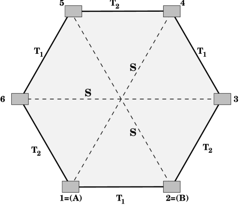
Figure 1: Alternate applications of T-duality in $y_{1}$ and $y_{2}$ directions lead to the same configuration after six operations. The diametrically opposed points are connected by the simple $S$ duality that exchanges $y_{1}$ and $y_{2}$ directions.

Assuming T-duality, the picture that seems to be emerging is shown in fig. 2. Near the corners of the square at $T_{3}\to 0$ (inside the shaded surfaces), namely $(R_{1},R_{2})\to(\infty,\infty)$, and the other two corners related by $T$ and $S$ duality, supermembrane theory is solvable and provides an eleven-dimensional description that incorporates not only the perturbative $(1,0)$ string states, but also the general $(q_{1},q_{2})$ oscillating quantum states (as well as the extra states of the membrane). Indeed, we have seen that left and right moving oscillations along the momentum direction of the 2-brane reproduce the full (BPS and non-BPS) tower of states of string theory, with the only exception of the sector $w_{0}=l_{1}=l_{2}=0$, that we do not know how to describe (this is related to the problem of existence of a normalizable ground state of the membrane Hamiltonian [40, 49]). The corners which are appropriate to the membrane representations of fig. 1 are obtained by demanding that the associated target torus area is large. Using the values of the respective radii, we obtain the distribution as in fig. 2.

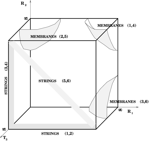
Figure 2: M-theory on ${\bf R^{9}}\times{\bf T}^{2}$. The sides of the cube correspond to either 0 or $\infty$ values of the different parameters, as indicated in the figure. Only the parameter space for a rectangular ($\tau_{1}=0$) torus is displayed. The diagonal string zone corresponds to $R_{1}R_{2}=\alpha^{\prime}$, arising, in particular, in the limit that led to eq. (87). The numbers between parentheses in the string zones indicate from what membrane such string description arises upon reduction in $y_{2}$.

At $T_{3}\to\infty$, various ten-dimensional limits can be taken, and we recover the string spectrum, as we have just seen. By using the full membrane Hamiltonian, in sect. 4 it was also shown that in the limit that the torus area goes to zero at fixed $\tau_{2}^{-1}\ll 1$, the only membrane quantum states of perturbative mass that remain are those of the superstring spectrum. The different string descriptions of figure 2 arise as follows. The horizontal edge is obtained by dimensionally reducing ${\rm(B)}=2$ or ${\rm(A)}=1$ along $y_{2}$ (as in eq. (84)); the string zone in the vertical edge follows from the reduction of membranes 3 or 4 along $y_{2}$ (as well as from (A) or 6 along $y_{1}$); the diagonal zone is obtained by reducing the membrane representations 5 and 6 along $y_{2}$ (as well as from 3 or (B) along along $y_{1}$, as in eq. (87) ).

5-branes are missing here. As in string theory –where there are soliton solutions representing higher-dimensional extended objects, but at weak coupling the $(1,0)$ string excitations are enough to define a sensible perturbation theory– in these corners of the moduli space, it is not impossible that the quantization of the 2-brane already provides the framework for perturbative calculations in M-theory on ${\bf R}^{9}\times{\bf T}^{2}$.

5 Conclusions

We conclude by summarizing the main topics discussed here:

$\bullet$ Several classical solutions representing (non-marginal) bound states of R-R and NS-NS $p$-branes admit a simple $d=11$ description as a reparametrization of configurations of 5 and 2 branes. In eleven dimensions, the background corresponding to a pure NS-NS configuration is no more complicated that the U-dual version including R-R and NS-NS $p$-branes.

$\bullet$ The quantum states (as derived from the light-cone Hamiltonian) of supermembranes wrapped on ${\bf R^{9}}\times{\bf T^{2}}$ that survive in the limit of small torus area, at fixed $\tau_{2}^{-1}\ll 1$, are those of the type II superstring spectrum on ${\bf R^{9}}\times S^{1}$, in the sector $w_{0}\neq 0$. For membranes on ${\bf R}^{10}\times S^{1}$, there remain extra quantum states.

$\bullet$ Correct BPS spectrum of the $(q_{1},q_{2})$ string bound state can be derived from a fundamental supermembrane, and in two inequivalent ways (corresponding to M2-brane backgrounds related by T-duality).

$\bullet$ Full dynamics of wrapped $d=11$ 2-branes can be understood in some corners of the moduli space, where supermembrane theory becomes exactly solvable.

$\bullet$ If T-duality is an exact symmetry of M-theory, boosted 2-branes with zero winding number (which are unstable) may be described in terms of a stable T-dual configuration.

I am grateful to M.J. Duff, K. Stelle and A.A. Tseytlin for useful and stimulating discussions. I would also like to thank the organizers of the APCTP Winter School on String Dualities for their kind hospitality.

References

• [1] J.H. Schwarz, hep-th/9607201.
• [2] J. Polchinski, hep-th/9611050.
• [3] M.J. Duff, hep-th/9611203; see also Proceedings of this conference.
• [4] P.K. Townsend, hep-th/9612121.
• [5] K.S. Stelle, hep-th/9701088.
• [6] A.A. Tseytlin, hep-th/9702163.
• [7] J.H. Schwarz, Phys. Lett. B360 (1995) 13 (E: B364 (1995) 252).
• [8] E. Witten, Nucl. Phys. B460 (1995) 335.
• [9] J.G. Russo and A.A. Tseytlin, Nucl. Phys. B (1997), hep-th/9611047.
• [10] G. Papadopoulos and P.K. Townsend, Phys. Lett. B380 (1996) 273, hep-th/9603087.
• [11] A.A. Tseytlin, Nucl. Phys. B475 (1996) 179.
• [12] I.R. Klebanov and A.A. Tseytlin, Nucl. Phys. B475 (1996) 179.
• [13] J. Gauntlett, D. Kastor and J. Traschen, hep-th/9604189.
• [14] G. Papadopoulos and P.K. Townsend, hep-th/9609095.
• [15] E. Bergshoeff, M. de Roo, E. Eyras, B. Janssen, and J.P. van der Schaar, hep-th/961209.
• [16] J. Gauntlett, G. Gibbons, G. Papadopoulos and P.K. Townsend, hep-th/9702202.
• [17] J.H. Schwarz, Nucl. Phys. B226 (1983) 269.
• [18] C. Hull and P. Townsend, Nucl. Phys. B438 (1995) 109.
• [19] P. Aspinwall, hep-th/9508154.
• [20] J.G. Russo, Phys. Lett. B (1997), hep-th/9701188.
• [21] J.C. Breckenridge, G. Michaud and R.C. Myers, hep-th/9611174.
• [22] M.S. Costa and G. Papadopoulos, hep-th/9612204.
• [23] J.G. Russo, Nucl. Phys. B (1997), hep-th/9610018 .
• [24] E. Bergshoeff, C. Hull and T. OrtΓ­n, Nucl. Phys. B451 (1995) 547.
• [25] A. Dabholkar, G.W. Gibbons, J. Harvey and F. Ruiz Ruiz, Nucl. Phys. B340 (1990) 33.
• [26] J.H. Horne, G.T. Horowitz and A.R. Steif, Phys. Rev. Lett. 68 (1992) 568.
• [27] G.T. Horowitz and A.A. Tseytlin, Phys. Rev. D51 (1994) 3351.
• [28] A. Dabholkar, J.P. Gauntlett, J.A. Harvey and D. Waldram, Nucl. Phys. B474 (1996) 85, hep-th/9511053.
• [29] M.J. Duff and K.S. Stelle, Phys. Lett. B253 (1991) 113.
• [30] A. Strominger and C. Vafa, Phys. Lett. B379 (1996) 99.
• [31] A.A. Tseytlin, Mod. Phys. Lett. A11 (1996) 689.
• [32] C.G. Callan and J.M. Maldacena, Nucl. Phys. B472 (1996) 571.
• [33] E. Bergshoeff, E. Sezgin and P.K. Townsend, Phys. Lett. B189 (1987) 75; Ann. Phys. 185 (1988) 330.
• [34] M.J. Duff, P.S. Howe, T. Inami and K.S. Stelle, Phys. Lett. B191 (1987) 70.
• [35] E. Bergshoeff, E. Sezgin and Y. Tanii, Nucl. Phys. B298 (1988) 187.
• [36] B. de Wit, J. Hoppe and H. Nicolai, Nucl. Phys. B305 [FS 23] (1988) 545.
• [37] D. Fairlie, P. Fletcher and C. Zachos, Phys. Lett. B218 (1989) 203; J. Hoppe, Int. J. Mod. Phys. A4 (1989) 5235; B. de Wit, U. Marquard and H. Nicolai, Commun.Math.Phys. 128 (1990) 39.
• [38] T. Banks, W. Fischler, S.H. Shenker and L. Susskind, hep-th/9610043.
• [39] R. Dijkgraaf, E. Verlinde and H. Verlinde, hep-th/9703030; H. Verlinde, see Proceedings of this conference.
• [40] B. de Wit, M. LΓΌscher and H. Nicolai, Nucl. Phys. B320 (1989) 135.
• [41] M.J. Duff, T. Inami, C. Pope, E. Sezgin and K. Stelle, Nucl. Phys. B297 (1988) 515.
• [42] A. Giveon, M. Porrati and E. Rabinovici, Phys.Β Rep. 244 (1994) 77.
• [43] M.J. Duff and J.X. Lu, Nucl. Phys. B347 (1990) 394.
• [44] E.Β Sezgin and R.Β Percacci, Mod. Phys. Lett. A10 (1995) 441.
• [45] P.K. Townsend, Phys. Lett. B373 (1996) 68.
• [46] O. Aharony, Nucl. Phys. B476 (1996) 470.
• [47] L. Susskind, hep-th/9611164.
• [48] O.J. Ganor, S.Β Ramgoolam and W.Β Taylor, hep-th/9611202.
• [49] J. FrΓΆhlich and J. Hoppe, hep-th/9701119.