LBNL-40109, UCB-PTH-97/13

hep-th/9703100

Dynamics of $N=2$ Supersymmetric Gauge Theories in Three Dimensions
Jan de Boer, Kentaro Hori and Yaron Oz

Department of Physics, University of California at Berkeley
366 Le Conte Hall, Berkeley, CA 94720-7300, U.S.A.
and
Theoretical Physics Group, Mail Stop 50A–5101
Ernest Orlando Lawrence Berkeley National Laboratory, Berkeley, CA 94720, U.S.A.

We study the structure of the moduli spaces of vacua and superpotentials of $N=2$ supersymmetric gauge theories in three dimensions. By analyzing the instanton corrections, we compute the exact superpotentials and determine the quantum Coulomb and Higgs branches of the theories in the weak coupling regions. We find candidates for non-trivial $N=2$ superconformal field theories at the singularities of the moduli spaces. The analysis is carried out explicitly for gauge groups $U(N_{c})$ and $SU(N_{c})$ with $N_{f}$ flavors. We show that the field theory results are in complete agreement with the intersecting branes picture. We also compute the exact superpotentials for arbitrary gauge groups and arbitrary matter content.

1 Introduction

In the past, relatively little effort was directed towards the study of $N=2$ supersymmetric gauge theories in three dimensions. In [2], pure $N=2$ $SU(2)$ supersymmetric Yang-Mills theory was studied and it was explained how instantons generate a superpotential $e^{-\Phi}$ in the effective action. The non-perturbatively generated superpotential for pure $SU(N_{c})$ gauge theory can be found by generalizing the results in [2]. The explicit result was first given in [3], who used M-theory along the line suggested in [4]. It was rederived in [5] in the context of intersecting brane configurations, along with results about mirror symmetry for $N=2$ theories. The aim of this paper is to study the moduli spaces of vacua and the non-perturbatively generated superpotentials of more general $N=2$ theories, in the weakly coupled regions. The results can be extrapolated to the strong coupling regions of the moduli spaces provided that the Kähler potential does not develop extra singularities.

The paper is organized as follows: In section 2 we introduce the basic properties of $N=2$ supersymmetric gauge theories in three dimensions. These theories have both Coulomb and Higgs branches. The former is parametrized by the vev’s of the bosonic degrees of freedom in the vector multiplet while the latter is parametrized by the vev’s of the scalars in the chiral multiplets. Due to $N=2$ supersymmetry both the Higgs and the Coulomb branches are Kähler manifolds. On the Coulomb branch the gauge group is generically broken to its maximal torus. This is in particular the case in the weakly coupled regions in which our studies are concentrated. In these regions the instanton calculus is reliable and we can study the non-perturbative generation of superpotentials.

One of the important results of section 2, which will be used in the later sections, is that the metric on the Coulomb branch of $N=2$ abelian gauge theories is completely determined at one loop. In order to show this we use the superspace formalism. The detailed form of the metric and complex structure of the Coulomb branch are found by performing a duality transformation in superspace. Another fundamental aspect of the structure that we find is that the quantum Coulomb branch degenerates at the points of massless electrons and consists of several branches. This can already be seen for abelian $N=2$ gauge theories as discussed in that section. However, the implications for the non-abelian cases are profound. In that case, different superpotentials are generated on different branches. In some branches, the superpotential may vanish. Due to the singularities, none of this contradicts holomorphy.

In section 3 we study the structure of the quantum Higgs and Coulomb branches and the non-perturbative generation of a superpotential for the gauge group $SU(2)$ with $N_{f}$ quarks in the fundamental representation. We show that the quantum Coulomb branch degenerates at the points of massless quarks and consists of several branches. We analyze in detail the non-perturbative generation of a superpotential depending differently on different branches. We find that a Higgs branch is not lifted by instanton corrections and is emanating from the singularity of the Coulomb branch, while at the singularity itself the Lagrangian description is not valid and the theory there is a candidate for a non-trivial $N=2$ superconformal field theory.

In section 4 we study the structure of the quantum Higgs and Coulomb branches and the non-perturbative generation of superpotentials for the gauge groups $U(N_{c})$ and $SU(N_{c})$ with $N_{f}$ quarks in the fundamental representation. The structure that we find generalizes that of the previous section. The quantum Coulomb branch develops singularitities separating different regions. We analyze in detail the non-perturbative generation of superpotentials in the different regions of the moduli space, as well as the structure of the Coulomb and Higgs branches and their intersections. We find many more candidates for non-trivial $N=2$ superconformal field theories. We review how the field theories can be obtained from an intersecting branes picture and show that the field theory results are in complete agreement with string theory results for the intersecting branes.

In section 5 we generalize the results to arbitrary gauge group and arbitrary matter content, and compute the exact superpotentials.

In the appendix we compute the number of fermionic zero modes of the $N=2$ theories in the background of monopoles which we use throughout the paper.

2 $N=2$ gauge theories in three dimensions

2.1 $N=2$ supersymmetry

$N=2$ supersymmetric gauge theories in three dimensions can be obtained by dimensionally reducing $N=1$ supersymmetric gauge theories in four dimensions. In this dimensional reduction the derivatives $\bar{D}_{\dot{\alpha}}$ and $D_{\alpha}$ become two complex conjugate derivatives $\bar{D}_{\alpha}$ and $D_{\alpha}$. To discuss the structure of the gauge multiplet it is convenient to consider the algebra of covariant derivatives, and it is here that there is a deviation between three and four dimensions. In three dimensions the algebra can be chosen to be of the form[6]

$$\{\nabla_{\alpha},\nabla_{\beta}\} = \{\bar{\nabla}_{\alpha},\bar{\nabla}_{\beta}\}=0$$

$${}\{\nabla_{\alpha},\bar{\nabla}_{\beta}\} = i\nabla_{\alpha\beta}+C_{\alpha\beta}G$$ (2.1)

where $\nabla_{\alpha\beta}$ is the vector derivative and $C_{\alpha\beta}$ is the second Pauli matrix $\sigma_{2}$. The field-strength $G$ is a linear superfield ($\nabla^{2}G=\bar{\nabla}^{2}G=0$), and its relation to the four-dimensional field strength is roughly $W_{\alpha}=\bar{D}_{\alpha}G$. In the chiral representation $\nabla_{\alpha}=e^{-V}D_{\alpha}e^{V},\bar{\nabla}_{\alpha}=\bar{D}_{\alpha}$, with $V$ an arbitrary Lie-algebra valued scalar superfield, the field strength $G$ reads $G=\bar{D}^{\alpha}(e^{-V}D_{\alpha}e^{V})$. It transforms covariantly under the gauge transformations $e^{V}\rightarrow e^{i\bar{\Lambda}}e^{V}e^{-i\Lambda}$.

The gauge kinetic term is now an integral over the full $N=2$ superspace,

$$S_{kin}=\frac{1}{2e^{2}}\int d^{3}xd^{2}\theta d^{2}\bar{\theta}{\rm Tr}(G^{2}).$$ (2.2)

Matter is included in the usual way,

$$S_{matter}=\int d^{3}xd^{2}\theta d^{2}\bar{\theta}(Q^{\dagger}e^{V}Q+\tilde{Q}e^{-V}\tilde{Q}^{\dagger}).$$ (2.3)

To avoid getting into issues of global ${\bf Z}_{2}$ anomalies and whether or not to include Chern-Simons terms, we will always take pairs of chiral superfields $Q,\tilde{Q}$, and count such a pair as one quark multiplet. There are two different kind of mass terms for quarks. There is a real mass term that can only be written in three-dimensional $N=1$ superspace and reads

$$S_{m}=\int d^{3}xd^{2}\theta^{\prime}(m_{r}Q^{\dagger}Q+\tilde{m}_{r}\tilde{Q}\tilde{Q}^{\dagger}),$$ (2.4)

where $d^{2}\theta^{\prime}$ is the measure for $N=1$ superspace, $d^{2}\theta^{\prime}=d^{2}(\theta+\bar{\theta})$. Again, to avoid anomalies, we will always take $m_{r}=-\tilde{m}_{r}$. Complex mass terms can be obtained directly from four dimensions and read

$$\int d^{3}xd^{2}\theta m_{c}\tilde{Q}Q+{\rm h.c.}$$ (2.5)

Finally, one may include Fayet-Iliopoulos terms $\zeta\int d^{3}xd^{2}\theta d^{2}\bar{\theta}V$ and superpotential terms $\int d^{3}xd^{2}\theta P(Q,\tilde{Q})+{\rm h.c.}$ in the action without destroying the $N=2$ supersymmetry.

2.2 Low energy effective action

The moduli space of vacua of $d=3,N=2$ gauge theories contains, in general, a Coulomb and an Higgs branch. By $N=2$ supersymmetry, both these moduli spaces are Kähler manifolds, but neither one of them is protected by some non-renormalization theorem against loop or non-perturbative corrections. The low-energy effective action is an $N=2$ supersymmetric sigma model that can be written as

$$S=\int d^{3}xd^{2}\theta d^{2}\bar{\theta}K(\Phi_{i},\bar{\Phi}_{i})+\int d^{3}xd^{2}\theta W(\Phi_{i})+{\rm h.c.},$$ (2.6)

where $K$ is the Kähler potential on the moduli space and $W(\Phi_{i})$ some superpotential. On the Higgs branch, the $\Phi_{i}$ are suitable gauge invariant combinations of the matter fields $Q,\tilde{Q}$. On the Coulomb branch, at a generic point, the gauge group is broken to a product of $U(1)$’s. If we denote by $\varphi$ the scalar and by $A_{\mu}$ the vector in the $N=2$ vector multiplet, then the action contains terms ${\rm Tr}[A_{\mu},A_{\nu}]^{2}$ and ${\rm Tr}[A_{\mu},\varphi]^{2}$. These should be zero for a supersymmetric vacuum, which shows that we can choose both $\varphi$ and $A_{\mu}$ to lie in a Cartan subalgebra of the gauge group. Part of the coordinates that parametrize the Coulomb branch are the vacuum expectation values $r_{i}=<\varphi_{i}>=<G_{i}>$. The other half of the coordinates are provided by the vacuum expectation values of scalar fields that one obtains by dualizing the gauge field in three dimensions. We will denote the scalar fields dual to the gauge fields by $\sigma_{i}$, and use the same symbol for its expectation value. The two real scalars $\varphi$ and $\sigma_{i}$ are related to the bosonic components of the chiral superfield $\Phi_{i}$ in (2.6). In the next section we will show explicitly how one performs the duality transformation to arrive at an action of the type (2.6), starting from the low-energy effective action in terms of the massless vector superfields $V_{i}$.

The Wilsonian effective action for the massless degrees of freedom on the Coulomb branch is obtained by integrating out all massive degrees of freedom, i.e. all charged matter multiplets and the off-diagonal components of the vector multiplets. The resulting effective action will be a functional of the remaining massless vector multiplets $V_{i}$, and in view of the gauge invariance of the effective action it will be a function of the field strengths $G_{i}$ of $V_{i}$ only. Since we are interested in the low-energy effective action, we will discard all terms in the action that contain derivatives of $G_{i}$ and keep only the part that is purely algebraic in $G_{i}$,

$$S_{{\rm low~{}energy}}=\int d^{3}xd^{2}\theta d^{2}\bar{\theta}f(G_{i}).$$ (2.7)

In general we expect arbitrary higher loop corrections in the function $f$. There are two important exceptions. First, if we are considering a theory with $N=4$ supersymmetry, we expect only a one-loop correction to $f$, but no higher loop corrections, although it may receive non-perturbative corrections. The second case is when the original gauge theory is abelian. In that case the action is bilinear in the massive fields, and the effective action has only a one-loop contribution. Furthermore, as there are no monopoles in an abelian gauge theory, nonperturbative corrections will be absent and the one-loop result is exact.

A similar analysis applies when there are neutral chiral multiplets $M$ in the theory. In that case, the low energy effective action will also include some of their degrees of freedom (which ones depends on the precise form of the superpotential), and more generally we have

$$S_{{\rm low~{}energy}}=\int d^{3}xd^{2}\theta d^{2}\bar{\theta}f(G_{i},M,\bar{M}).$$ (2.8)

Rather than computing the one-loop corrections to $f$, we will find it more convenient to first perform a duality transformation. The one-loop corrections in the dual variables are already known [7, 8], and by performing an inverse duality transformation one may easily obtain the one-loop corrections to $f$.

2.3 Duality transformation

To perform the duality transformation, consider [6]

$$S=\int d^{3}xd^{2}\theta d^{2}\bar{\theta}(f(\tilde{G}_{i},M,\bar{M})-\tilde{G}_{i}(\Phi_{i}+\bar{\Phi}_{i})),$$ (2.9)

where the $\tilde{G}_{i}$ are unconstrained real superfields, and the $\Phi_{i}$ are chiral superfields. By varying $\Phi_{i}$ we find that $\tilde{G}_{i}$ is a linear superfield and substituting this in the action we reobtain (2.8). Another possibility is to vary the action with respect to $\tilde{G}_{i}$. This leads to the equation

$$\Phi_{i}+\bar{\Phi}_{i}=\frac{\partial f(\tilde{G}_{i},M,\bar{M})}{\partial\tilde{G}_{i}}.$$ (2.10)

By solving this for $\tilde{G}_{i}$ in terms of $\Phi_{i}+\bar{\Phi}_{i}$, and substituting this back into the action (2.9), we obtain the dual description

$$S=\int d^{3}xd^{2}\theta d^{2}\bar{\theta}K(\Phi_{i}+\bar{\Phi}_{i},M,\bar{M}),$$ (2.11)

where $K$ is the Legendre transform of $f$. The action (2.11) is the standard action for a set of chiral superfields, and the moduli space is the complex manifold parametrized by the vevs of $\Phi_{i}$ with Kähler potential $K$. Even if $f$ has only one-loop corrections, $K$ will have corrections to all orders in the coupling constant, due to the fact that one has to invert the relation (2.10).

The duality transformation, when worked out in components, contains the usual duality transformation to go from a gauge field to a scalar $\sigma$. This scalar is the imaginary scalar component of the superfield $\Phi$. As one can see by considering Wilson lines for the gauge field, the scalar $\sigma$ should be compact. With the normalizations above, this means that we have to identify

$$\Phi\sim\Phi+2\pi i\lambda_{k}$$ (2.12)

for each fundamental weight $\lambda_{k}$ of the Lie algebra of the gauge group. In other words, $\Phi$ is a multivalued coordinate on the moduli space, and the good single valued superfields are $e^{\alpha_{i}\cdot\Phi}$, where $\alpha_{i}$ is a simple root. These superfields also provide the natural complex structure on the moduli space. This already severely constrains the form of a superpotential: it must be a holomorphic function of $e^{\alpha_{i}\cdot\Phi}$.

The action (2.11) is obviously invariant under constant shifts of $\sigma$. In view of the compactness of $\sigma$, these constant shifts form ${\rm rank}(G)$ commuting holomorphic $U(1)$ isometries of the metric on the moduli space. These symmetries cannot be broken in perturbation theory, but can be broken by a non-perturbatively generated superpotential.

Finally it is important to notice that due to the identity (2.10) the relation between $<\Phi_{i}>$ and $r_{i}\equiv<G_{i}>$ can be quite complicated. This will play a crucial role later on in order that the non-perturbative superpotential that we find is not in conflict with results from index theory, but does in fact confirm these results. It will turn out that the chiral superfields $\Phi_{i}$ are not always good coordinates on the Coulomb branch. Their real part may become $-\infty$, and if this happens we have to consider different coordinate patches to discuss the Coulomb branch. This allows for the possibility to have different superpotentials on different pieces of the Coulomb branch, without violating holomorphy. In the sequel, we will see how this will enable us to arrive at a consistent picture for the dynamics on the Coulomb branch of $N=2$ theories with arbitrary matter.

2.4 Example: $U(1)$ with one flavor

The one-loop metrics described in [7, 8] were expressed in the ‘mixed’ variables $r_{i}=<G_{i}>$ and $\sigma_{i}={\rm Im}(<\Phi_{i}>)$. To illustrate how one derives such a metric in the above picture we will discuss as an example the case of a $U(1)$ gauge theory with one electron. The one-loop metric in this case reads

$$ds^{2}=\frac{1}{4}\left(\frac{1}{e^{2}}+\frac{1}{|r|}\right)dr^{2}+\left(\frac{1}{e^{2}}+\frac{1}{|r|}\right)^{-1}d\sigma^{2}$$ (2.13)

Classically, the moduli space is a cylinder, but quantum mechanically it is broken up in two pieces ($r>0$ and $r<0$), that both look like a rounded-off half-cylinder. Both half-cylinders touch at a point. At this point we can neglect $1/e^{2}$ and the metric looks like that of two complex planes touching at the origin, $ds^{2}\sim dzd\bar{z}$ with $z=\sqrt{|r|}e^{i\sigma}$. The difference between the tree-level and one-loop metric is illustrated in figure 1.

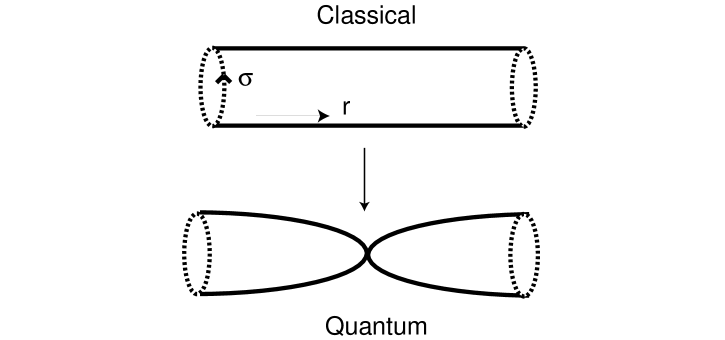
Figure 1: The classical and quantum moduli spaces of vacua of $U(1)$ theory.

The one-loop low-energy effective action for this theory reads

$$f(G)=\frac{1}{2e^{2}}G^{2}+G\log(G/e^{2})$$ (2.14)

and from (2.10) we obtain the relation between $\Phi$ and $G$,

$$\Phi=\frac{1}{2e^{2}}G+\frac{1}{2}\log(G/e^{2})+\frac{1}{2}+i\sigma.$$ (2.15)

The sigma-model metric of the dualized theory reads

$$ds^{2}=K^{\prime\prime}(\Phi+\bar{\Phi})d\Phi d\bar{\Phi}$$ (2.16)

where we denote by $\Phi$ both the superfield and its vev. To express $ds^{2}$ in terms of $r=<G>$ and $\sigma$ we use the fact that the inverse of a Legendre transform is again a Legendre transform, and therefore

$$K^{\prime}(\Phi+\bar{\Phi})=r.$$ (2.17)

Differentiating once more, we find

$$K^{\prime\prime}(\Phi+\bar{\Phi})=\left(\frac{\partial(\Phi+\bar{\Phi})}{\partial r}\right)^{-1}=\left(\frac{1}{e^{2}}+\frac{1}{r}\right)^{-1}.$$ (2.18)

Thus, for the metric we finally get

$$ds^{2}=\left(\frac{1}{e^{2}}+\frac{1}{r}\right)^{-1}\left(\frac{1}{2}\left(\frac{1}{e^{2}}+\frac{1}{r}\right)dr+id\sigma\right)\left(\frac{1}{2}\left(\frac{1}{e^{2}}+\frac{1}{r}\right)dr-id\sigma\right),$$ (2.19)

which indeed agrees with (2.13). This is the exact result, and by expanding it in powers of $e^{2}$ one can see that it does contain terms with arbitrary high powers of $e^{2}$. However, beyond one-loop they are all a result of the duality transformation.

In this simple case we already see the phenomenon that the chiral superfield $\Phi$ is not a good coordinate everywhere on the moduli space. Its real part becomes $-\infty$ as we approach the point $r=0$ where the electron becomes massless, and the moduli space decomposes in two different parts, only half of which is described by $\Phi$. A priori, there can be different non-perturbative dynamics on each part of the moduli space, without violating holomorphy, and we will see in examples of non-abelian gauge theories that this is indeed what happens.

2.5 General abelian gauge theories

We will now discuss the case of a general abelian gauge theory, with gauge group $U(1)^{N_{c}}$, and $N_{f}$ electrons $Q_{a},\widetilde{Q}_{a}$, with charges $q_{ia}$ under the $i$-th $U(1)$ gauge group. In addition, we will assume that the electrons have a real mass $m_{r}^{a}$ and that there are superpotential terms $\int d^{3}xd^{2}\theta m_{c}^{a}\widetilde{Q}_{a}Q_{a}$. The metric in terms of $r_{i}$ and $\sigma_{i}$, $i=1\ldots N_{c}$ can be extracted from the results in [9]. We will be mainly interested in the relation between $\Phi_{i}$ and $r_{i}$, and it is this relation that we will compute here. According to the discussion above, the second derivative of $K$ yields directly the coefficient in front of $d\sigma_{i}d\sigma_{j}$ in the metric on the moduli space. On the other hand, the second derivative of $K$ is proportional to $\partial r_{j}/\partial(\Phi_{i}+\bar{\Phi}_{i})$. Combining these observations with the results of [9] we obtain

$$\frac{\partial(\Phi_{i}+\bar{\Phi}_{i})}{\partial r_{j}}=\frac{\delta_{ij}}{e^{2}}+\sum_{a}\frac{q_{ia}q_{ja}}{\sqrt{(\sum_{k}q_{ka}r_{k}-m_{r}^{a})^{2}+|m_{c}^{a}|^{2}}}.$$ (2.20)

This can be integrated to yield

$$\Phi_{i}=\frac{r_{i}}{2e^{2}}+\frac{1}{2}\sum_{a}q_{ia}\log\left(\sum_{k}q_{ka}r_{k}-m_{r}^{a}+\sqrt{(\sum_{k}q_{ka}r_{k}-m_{r}^{a})^{2}+|m_{c}^{a}|^{2}}\right)+i\sigma_{i}.$$ (2.21)

The one-loop result for a general non-abelian gauge theory has a similar form, with an extra term

$$-\frac{1}{4}\sum_{b}q_{ib}\log\left(\sum_{k}q_{kb}r_{k}\right)$$ (2.22)

in the right hand side of (2.21), where $q_{ib}$ are the $U(1)$ charges of the various massive vector bosons labeled by $b$.

2.6 Preliminary remarks on non-abelian gauge theories

In the following sections, we analyze non-abelian gauge theories. The essential difference between abelian and non-abelian gauge theories is that non-perturbative effects are present in non-abelian gauge theories because of instanton configurations, which are BPS monopoles from the four-dimensional point of view. In particular, a superpotential can be generated only by such non-perturbative effects. To determine whether or not a particular monopole configuration can contribute to the superpotential we use zero mode counting and the $U(1)_{R}$ symmetry. The number of fermionic zero modes in a monopole background is determined by the index of the corresponding Dirac operator. This index is computed in the Appendix. The results for $SU(N_{c})$ gauge theory with $N_{f}$ quark multiplets, i.e., $N_{f}$ pairs of chiral multiplets in the fundamental and the dual representation, are as follows. Let us consider a magnetic monopole in the unbroken gauge group $U(1)^{N_{c}-1}$ of magnetic charge $(n_{1},n_{2},\ldots,n_{N_{c}-1})$. In this configuration, there are $2\sum n_{i}$ zero modes from gluinos. The number of zero modes from quark multiplets depends on the vev of the scalar field $\varphi={\rm diag}(r_{1},\ldots,r_{N_{c}})$. By using the Weyl group action, we may assume that $r_{i}>r_{i+1}$. Let us focus on the $a$-th quark. If its real bare mass is in the interval $r_{i}>m_{r}^{a}>r_{i+1}$ for some $i$, it has $2n_{i}$ zero modes. If its real bare mass is larger than $r_{1}$ or smaller than $r_{N_{c}}$, there are no zero modes. We will not discuss the other cases in which some $r_{i}$ coincide with $m_{r}^{a}$. Since gluinos have $U(1)_{R}$ charge $+1$ and fermions in quark multiplets have charge $-1$, a superpotential can be generated by instantons in this sector only when

$$2\sum_{i=1}^{N_{c}-1}n_{i}-2\sum_{a=1}^{N_{f}}\ell_{a}=2$$ (2.23)

where $\ell_{a}:=n_{i}$ if $r_{i}>m_{r}^{a}>r_{i+1}$ and $\ell_{a}=0$ if $m_{r}^{a}>r_{1}$ or $m_{r}^{a}<r_{N_{c}}$. If there is no complex mass and the quark vevs all vanish there are additional global $U(1)$ symmetries. In particular, a combination of $U(1)_{R}$ and the axial $U(1)$ flavor symmetry leads to the additional selection rule

$$2\sum_{i=1}^{N_{c}-1}n_{i}+2\sum_{a=1}^{N_{f}}\ell_{a}=2.$$ (2.24)

An interesting consequence of the above formula is that instanton sectors that may possibly contribute to the superpotential can change as $\varphi$ is varied, e.g., as we move from $r_{i}>m_{r}^{a}$ to $r_{i}<m_{r}^{a}$. This suggests that the superpotential can jump along real codimension one hypersurfaces $r_{i}=m_{r}^{a}$ of the Coulomb branch, which seems peculiar in view of the fact that the superpotential should be a holomorphic function of the chiral multiplets. The resolution of this as we will observe in the following sections is that the Coulomb branch degenerates along the hypersurfaces which actually have complex codimension one and consists of several branches, on each of which the superpotential is holomorphic. This degeneration is caused by loop corrections to the metric. In fact, near the “phase boundary” $r_{i}=m_{r}^{a}$, the theory can be well approximated by the $U(1)$ gauge theory with a single electron (tensored with the remaining free $U(1)^{N_{c}-2}$ maxwell theory), and we know the behavior of the Coulomb branch of such a theory near the point of a massless electron. As discussed in section 2.4, it is exactly determined at the one-loop level, and the structure of degeneration is depicted in Figure 1.

In the following sections we will always consider the weakly coupled region of the moduli space, i.e. the region where $|r_{i}-r_{j}|\gg e^{2}$. In this region, the off-diagonal components of the vector multiplet are very heavy and the theory can be approximated by an abelian gauge theory with $N_{c}N_{f}$ electrons. The abelian theory has only one-loop corrections, and this is the reason that the one-loop results are an accurate description of the moduli space at weak coupling. The results can be extrapolated to the strong coupling regions provided we assume that the Kähler potential does not develop extra singularities there.

3 Dynamics of $SU(2)$ Gauge Theories

In this section, we determine the structure of vacua in the weak coupling region of $SU(2)$ gauge theories with matter chiral multiplets in the fundamental representation. In particular, we will see how the classical Coulomb branch degenerates to have several branches due to one loop effects and how one of them is lifted due to the non-perturbative generation of a superpotential.

The classical Coulomb branch is parametrized by the vevs of the scalar field $r$ of the vector multiplet in the unbroken $U(1)$ subgroup and the scalar $\sigma$ dual to the $U(1)$ vector field. The classical metric looks like

$$ds^{2}={1\over 4e^{2}}dr^{2}+e^{2}d\sigma^{2}.$$ (3.1)

It is the cylinder $\{(r,\sigma)\}$; $\sigma\equiv\sigma+2\pi$ divided by the action of the Weyl goup $(r,\sigma)\mapsto(-r,-\sigma)$. As we increase the vev $|r|$, loop and instanton corrections to (3.1) and other physical quantities decrease as inverse powers of $r/e^{2}$ and exponentially $\,\,{\rm e}^{-|r|/e^{2}}$ respectively. Conversely, if we decrease $|r|$ below $e^{2}$ we expect a strong dynamics involving gluons and gluinos. For instance, the one-loop corrected metric of the pure Yang-Mills theory is $ds^{2}=gdr^{2}/4+g^{-1}d\sigma^{2}$ where

$$g={1\over e^{2}}-{2\over|r|}\,.$$ (3.2)

We observe that below $|r|=2e^{2}$ the one-loop metric becomes negative definite and higher loop and instanton corrections are needed to render the metric positive definite. This is the analog of the QCD scale $\Lambda$ in four-dimensional asymptotically free gauge theories where the one-loop gauge coupling constant diverges. In what follows, we focus on the weak coupling region $|r|\gg e^{2}$ in which the semi-classical approximation is valid. By using the Weyl group action, we can restrict attention to the region $r\gg e^{2}$. We also assume that all the real bare masses of the quarks are much greater than $e^{2}$ so that there are no massless quarks in the strong coupling region.

A superpotential can be generated only by non-perturbative effects. Since we are considering the region $r\gg e^{2}$ where we do not expect strong dynamical effect, a superpotential can be generated only by instantons, which are the magnetic monopoles in the unbroken $U(1)$ subgroup of $SU(2)$. A superpotential is generated only when a selection rule coming from a conserved fermion number symmetry $U(1)_{R}$ is satisfied. Under this $U(1)_{R}$ global symmetry, the “gluinos” (fermions in the $SU(2)$ vector multiplet) have charge $+1$ and the fermions in the matter chiral multiplet have charge $-1$, and a possible F-term carries charge $2$.

To see whether the superpotential is generated, we need to count the number of fermion zero modes of Dirac operator in the instanton configuration. The results are summarized in section 2.6. In the configuration of magnetic charge $n$, there are $2n$ zero modes from gluinos. The number of fermion zero modes in the matter chiral multiplet depends on the vev $r$. From each quark multiplet, there are $2n$ zero modes if $r$ is larger than the real bare mass $m_{r}$, while there are no zero modes if $r<m_{r}$. Thus, the selection rule is now expressed as

$$2n-2nk=2\,,$$ (3.3)

where $k$ is the number of quarks whose real bare masses are smaller than $r$. There is a solution ($n=1$) only when $k=0$. Namely, a superpotential can be generated only when $r$ is smaller than any of the real bare masses, and it is by a one-instanton effect.

3.1 Pure Yang-Mills Theory

Let us consider the case of pure $N=2$ $SU(2)$ Yang-Mills theory. In view of the above analysis, a superpotential may be generated. In fact, it was first shown in [2] that it is indeed generated. Using the dilute instanton gas approximation one finds it has the form [2]

$$W=\,\,{\rm e}^{-\phi}\,,$$ (3.4)

where $\phi$ is the chiral multiplet dual to the linear multiplet whose lowest component is the complex scalar field of the form $\phi=I+i\sigma$. Here, $I$ depends on $r$ and approaches the classical lagrangian $r/2e^{2}$ in the limit $r/e^{2}\rightarrow\infty$. Thus in the weak coupling region, the Coulomb branch is completely lifted and there is no supersymmetric vacuum.

3.2 The Single Flavor Case

Let us next consider the case with a single quark multiplet. From the above selection rule (3.3), when the complex bare mass is turned off $m_{c}=0$, a superpotential may be generated in the region $r<m_{r}$ but is never generated when $r>m_{r}$. If we send $m_{r}$ to infinity, we expect to recover the superpotential (3.4) of pure $N=2$ Yang-Mills theory. It implies that a superpotential is non-zero in the region $r<m_{r}$ and is zero when $r>m_{r}$. This seems peculiar because the superpotential is a holomorphic function but a holomorphic function vanishing on one region must be vanishing everywhere. If the Coulomb branch is like the classical half-cylinder (3.1), there must be a jump of the superpotential on the “phase boundary” $C=\{r=m_{r},0\leq\sigma\leq 2\pi\}$ of real codimension one, which should not be the case.

As mentioned in section 2.6, the only possible resolution to this puzzle is that the Coulmb branch degenerates to have at least two branches and the superpotential is non-zero on one branch and is zero on the other. As we now see, this is actually the case. The “phase boundary” $C$ shrinks to a point.

Note that in the limit $r,m_{r}\gg e^{2}$, $|r-m_{r}|\,\,\displaystyle{\mathop{<}_{\sim}}\,\,e^{2}$, the off-diagonal pieces of the $SU(2)$ vector multiplet (W-bosons and their superpartners) decouple and we can well approximate the system by an $N=2$ $U(1)$ gauge theory with $N_{f}=1$ electron. As discussed in the previous section, the Coulomb branch of the latter system is determined at the one loop level and the metric is given by (2.19) in which we identify $r$ with $r-m_{r}$. It behaves in the limit $|r-m_{r}|/e^{2}\rightarrow 0$ as

$$ds^{2} = {1\over 4|r-m_{r}|}dr^{2}+|r-m_{r}|d\sigma^{2}$$ (3.5)

$$= \left(d\sqrt{|r-m_{r}|}\right)^{2}+\sqrt{|r-m_{r}|}^{2}d\sigma^{2}\,.$$

From this expression we see that the “phase boundary” $C$ = $\{r=m_{r},0\leq\sigma\leq 2\pi\}$ has shrunk to a point and the Coulomb branch has degenerated to have two branches corresponding to $r\leq m_{r}$ and $r\geq m_{r}$. The metric (3.5) on each branch is the flat metric on the complex line with the coordinate $x=\sqrt{m_{r}-r}\,\,{\rm e}^{-i\sigma}$ for the branch $r\leq m_{r}$ and $y=\sqrt{r-m_{r}}\,\,{\rm e}^{i\sigma}$ for $r\geq m_{r}$. Note that this region of the Coulomb branch is simply described by

$$xy=0\,,$$ (3.6)

as has already been seen in [5]. A Higgs branch is emanating from the singular point $x=y=0$. Classically, it is described by the Kähler quotient of ${\bf C}\oplus{\bf C}^{\vee}$ by the $U(1)$ action (with vanishing FI parameter in this case), and is the orbifold ${\bf C}/{\bf Z}_{2}$ of deficit angle $\pi$ at the origin which is the intersection point with the Coulomb branch.

When the complex bare mass is turned on $m_{c}\neq 0$, the description (3.6) changes to

$$xy=m_{c}\,,$$ (3.7)

and the singularity at $x=y=0$ is deformed to be smooth. Due to the tree level superpotential $m_{c}\widetilde{Q}Q$ the Higgs branch is lifted.

Now, we complete the description of vacua in this weak coupling region by taking into account the non-perturbative superpotential. From the zero mode counting and by considerating the limit $m_{r}\rightarrow\infty$, we expect in the case $m_{c}=0$ that the one-instanton configurations generate the superpotential $W=\exp(-I-i\sigma)$ in the branch $r\leq m_{r}$. In the branch $r\geq m_{r}$ the superpotential is not generated, $W=0$. In the limit $m_{c}\rightarrow\infty$, we also expect to obtain the superpotential (3.4). The superpotential with this property is uniformly expressed as

$$W=\,\,{\rm e}^{-\phi}$$ (3.8)

where $\phi$ is a chiral superfield whose scalar component is a holomorphic function on the Coulomb branch such that ${\rm Im}\phi=\sigma$. In the particular region of interest, $\phi$ is approximately the one given in terms of $r$ and $\sigma$ by (2.21) applied to the case of $U(1)$ gauge theory with electrons of charge $\pm 1$. In other words, the superpotential has the lowest component

$$W = \,\,{\rm e}^{-{r\over 2e^{2}}-i\sigma}\left(\frac{(-r-m_{r})+\sqrt{(-r-m_{r})^{2}+|m_{c}|^{2}}}{(r-m_{r})+\sqrt{(r-m_{r})^{2}+|m_{c}|^{2}}}\right)^{1/2}$$ (3.9)

$$\sim \,\,{\rm e}^{-{r\over 2e^{2}}-i\sigma}\left(\frac{|m_{c}|^{2}}{(r-m_{r})+\sqrt{(r-m_{r})^{2}+|m_{c}|^{2}}}\right)^{1/2}$$

Indeed, in the limit $m_{c}\rightarrow 0$, $W=0$ for $r>m_{r}$ and $W=\sqrt{m_{r}-r}\,\,{\rm e}^{-{r\over 2e^{2}}-i\sigma}$ for $r<m_{r}$. Also, in the limit $m_{c}\rightarrow\infty$, it becomes $\,\,{\rm e}^{-{r\over 2e^{2}}-i\sigma}$. Note that near the singularity $r=m_{r}$ of the $m_{c}=0$ model, the superpotential behaves in the branch $r\leq m_{r}$ as

$$W=\,\,{\rm e}^{-\phi}\sim\sqrt{m_{r}-r}\,\,{\rm e}^{-i\sigma}=x\,.$$ (3.10)

We can modify the definition of $x$ to be $x=\,\,{\rm e}^{-\phi}$ so that $W=x$ is exact for all values of $m_{r}$ and $m_{c}$. When $m_{c}=0$, since $\partial W/\partial x=1$ and $ds^{2}=dxd\overline{x}$ near the point $x=0$, the branch $r\leq m_{r}$ is completely lifted (except for possible vacua in the strong coupling region which is not under control). The branch $r\geq m_{r}$ remains as supersymmetric vacua. When the complex bare mass is turned on $m_{c}\neq 0$, the Coulomb branch is described by $xy=m_{c}$, and as $\partial W/\partial x=1$ and $\partial W/\partial y=-m_{c}y^{-2}$, the whole Coulomb branch is lifted.

The Higgs branch, which is classically present for $m_{c}=0$, may possibly be lifted by the generation of a superpotential. Here we exclude this possibility. In this situation, a superpotential can only be generated by instantons. Thus, it must be a chiral superfield containing a power of $\,\,{\rm e}^{-i\sigma}$. Namely, it must contain a positive power of $\,\,{\rm e}^{-\phi}$. However, $\,\,{\rm e}^{-\phi}$ vanishes at $r=m_{r}$ where the Higgs branch is emanating. This shows that there is no dynamical generation of superpotential on the Higgs branch. The metric on the Higgs branch may be corrected by non-perturbative effects, but the correction is very small in the region $r=m_{r}\gg e^{2}$.

It is a subtle issue whether the point $x=y=0$ intersecting with the Higgs branch corresponds to a supersymmetric vacuum. The derivative of the superpotential $W$ is vanishing in the directions of Higgs branch and of the component $r\geq m_{r}$ of the Coulomb branch but is non-vanishing in the direction of the branch $r\leq m_{r}$. However, we should note that the lagrangian description in terms of the variables we have used is not valid at this point. Thus, there is no reason to exclude this point from the set of vacua. If it is really a supersymmetric vacuum, it may correspond to a non-trivial $N=2$ superconformal field theory.

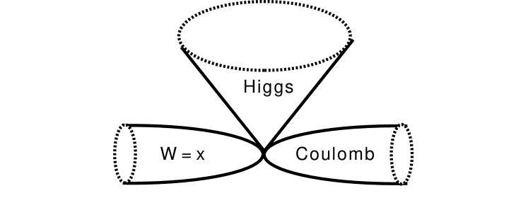
Figure 2: The moduli space of vacua at weak coupling.

To summarize, the $SU(2)$ gauge theory with one quark multiplet of large real bare mass $m_{r}\gg e^{2}$ and vanishing $m_{c}=0$ has two branches in the weak coupling region: one is a Higgs branch with a conical singularity and the other is a Coulomb branch. They might intersect at one point, as in figure 2. When $m_{c}$ is turned on, both the Higgs and Coulmb branches are lifted completely.

Notice that we did not take instanton corrections to the Kähler potential into account. If such corrections exist and are e.g. of the form $|e^{-\Phi}|^{2}$, with $\Phi$ the holomorphic field on the Coulomb branch $r>m_{r}$, they may diverge as $r\downarrow m_{r}$ and change the picture. In [15] it was argued that the Coulomb and Higgs branches merge. If that is the case they are connected by an exponentially small neck that vanishes as $m_{r}\rightarrow\infty$, and figure 2 applies to this limit.

3.3 The Multi-Flavor Case

For the case with $N_{f}>1$, the analysis is similar and hence we present only the result. As noted previously, we assume that all the real mass parameters are much larger than $e^{2}$, $m_{r}^{a}\gg e^{2}$. The Coulomb branch degenerates at each point $r=m_{r}^{a}$ such that $m_{c}^{a}=0$, and from these points a Higgs branch emanates. If the number of massless quark multiplets is one, the local structure of the moduli space is of course the same as in the $N_{f}=1$ case. If there are $N$ massless quarks at a point, i.e., if $N$ quarks have the same real mass and vanishing complex mass parameters, the Coulomb branch degenerates at the point and locally looks like two cones of the type ${\bf C}/{\bf Z}_{N}$ intersecting at the origin. The Higgs branch emanating from this point is the singular subspace of ${\bf C}^{N^{2}}=\{x_{a,b}\}$ defined by $x_{a,b}x_{c,d}=x_{a,d}x_{c,b}$ which has a complex dimension $2N-1$. The superpotential is uniformly written as

$$W=\,\,{\rm e}^{-\phi}\sim\,\,{\rm e}^{-{r\over 2e^{2}}-i\sigma}\prod_{a=1}^{N_{f}}\left(\frac{|m_{c}^{a}|^{2}}{r-m_{r}^{a}+\sqrt{(r-m_{r}^{a})^{2}+|m_{c}^{a}|^{2}}}\right)^{1/2}.$$ (3.11)

Note that the superpotential is vanishing in the branches in $r\geq m_{r}^{a_{0}}$ where $m_{r}^{a_{0}}$ is the smallest $m_{r}^{a}$ such that $m_{c}^{a}=0$, and non-vanishing in the branch $r\leq m_{r}^{a_{0}}$. If all the complex bare masses are non-zero, then, $W$ is nowhere vanishing.

Near the region ${\rm min}\{m_{r}^{a}\}\leq r\leq{\rm max}\{m_{r}^{a}\}$, the Coulomb branch is holomorphically embedded in an ALE space, which is a resolution of the complex surface described by

$$xy=\prod_{a=1}^{N_{f}}\,\,(z-m_{c}^{a}).$$ (3.12)

The parameter of resolution is encoded in $m_{r}^{a}$. Roughly speaking, when $m_{c}^{a}$ are very small, there are $N_{f}-1$ two-spheres whose intersection matrix is the Cartan matrix of $A_{N_{f}-1}$ type, and the size of the $a$-th sphere is given by the difference $m_{r}^{a}-m_{r}^{a+1}$ of the neighboring real masses. The embedding of the Coulomb branch is defined by

$$z=0\,.$$ (3.13)

The superpotential is expressed as

$$W=x\,.$$ (3.14)

If all the complex masses are turned on, the Coulomb branch, being described by $xy=$non-zero constant, has a good coordinate $x$, and it is lifted because $\partial W/\partial x=1$. It is possible to see that the superpotential (3.14) behaves as mentioned above as we turn off some complex mass parameters.

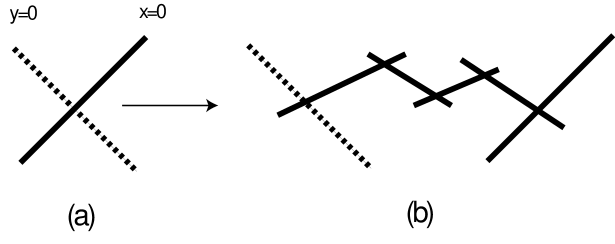
Figure 3: Coulomb branches of $SU(2)$ gauge theories.

As an ilustration, we present in figure 3 the Coulomb branch for the case in which all the complex mass parameters are turned off. Figure 3(a) describes the case in which all the real masses are the same and 3(b) is for the case in which they are distinct. The dashed lines are the branches that are lifted by the superpotential (3.14), and the solid lines are the branches that remain as supersymmetric vacua because (3.14) vanishes identically on them. Intermediate branches in fig 3(b) are ${\bf P}^{1}$’s whose sizes are given by the difference of the neighboring real mass parameters. In the scenario of [15], the Coulomb branch that connects to the dashed line in figure 3(b) is merged with a Higgs branch.

4 Dynamics of $U(N_{c})$ Gauge Theories

In this section we will study the superpotentials and the structure of the moduli spaces of vacua for gauge groups $U(N_{c})$ and $N_{f}$ pairs of chiral multiplets in the fundamental representation. The analysis and the structure that we will find generalizes that of the previous section. The case of $SU(N_{c})$ gauge groups follows in a straightforward way from the analysis for $U(N_{c})$ gauge groups and we will outline the differences.

As discussed previously, the bosonic part of the $N=2$ vector multiplet contains the three dimensional gauge field $A_{\mu}$ and a real scalar $\varphi$ corresponding to the $A_{4}$ component of the four dimensional gauge field. The terms $Tr[A_{\mu},A_{\nu}]^{2}$ and $Tr[A_{\mu},\varphi]^{2}$ in the $N=2$ action imply that the Coulomb branch of the theory is parametrized by the vev’s of the scalars $\varphi_{i}$ taking values in the Cartan sub-algebra of the gauge group and the the scalars $\sigma_{i}$ dual to the photons. The scalars in the quark multiplets parametrize the Higgs branch of the theory.

The metrics on the moduli spaces of vacua receive both loop and non perturbative corrections. A superpotential can only be generated non perturbatively. As discussed previously, one expects the non-perturbative effects to come only from instantons which are monopoles in three dimenions. Their magnetic charges correspond to the simple roots of the Lie algebra. The regions of weak coupling are defined by $|r_{i}-r_{j}|\gg e^{2}$. In these regions the instanton factor is small and the instanton calculus is reliable.

4.1 $U(3)$ Gauge Group

In this subsection we will analyse the $N=2$ supersymmetric gauge theories with gauge group $U(3)$. We will consider first the case with no quarks $N_{f}=0$.

4.1.1 Pure Yang-Mills Theory

The classical metric on the Coulomb branch is

$$ds^{2}=\sum_{i=1}^{3}\left(\frac{1}{4e^{2}}dr_{i}^{2}+e^{2}d\sigma_{i}^{2}\right)\mskip 6.0mu,$$ (4.1)

where $\sigma_{i}$ are periodic with period $2\pi$. The classical moduli space of vacua is that of three cylinders $\{r_{i},\sigma_{i}\}$ modded out by by the action of the Weyl group.

This metric receives loop and instanton corrections. In order to see whether the moduli space of vacua is lifted or not we have to check whether a superpotential is generated. The index formula for the fermionic zero modes in the background of a monopole of a charge vector $(n_{1},n_{2})$ takes the form

$$2(n_{1}+n_{2})=2\mskip 6.0mu.$$ (4.2)

Therefore only the fundamental monopoles with charge vectors $(1,0)$ and $(0,1)$ contribute to the superpotential. The corresponding instanton terms are $\,\,{\rm e}^{-(\phi_{1}-\phi_{2})}$ and $\,\,{\rm e}^{-(\phi_{2}-\phi_{3})}$ respectively. The superpotential reads

$$W=\,\,{\rm e}^{-(\phi_{1}-\phi_{2})}+\,\,{\rm e}^{-(\phi_{2}-\phi_{3})}\mskip 6.0mu.$$ (4.3)

Thus, in the weak coupling region the Coulomb branch is completely lifted at the quantum level.

4.1.2 The Single Flavor Case

Consider now adding one quark, namely $N_{f}=1$. Each quark generates two fermionic zero modes with opposite sign to the gluino zero modes. However when the complex mass parameter $m_{c}$ of the quark is diferent than zero the two extra zero modes are lifted. Thus the superpotential generated in the case with one quark and $m_{c}\neq 0$ is the same as that with no quark multiplets (4.3), and the classical moduli space of vacua is lifted by instantons.

Consider now the case with $m_{c}=0$. Without loss of generality we consider the region $r_{1}>r_{2}>r_{3}$. The other regions can be analyzed similarly, or alternatively can be obtained by the action of the Weyl group. In order to analyze the possible monopoles contributing to the superpotential we have to distinguish between several regions depending on the real mass parameter $m_{r}$ of the quark.

(1) $r_{1}<m_{r}$ or $r_{3}>m_{r}$: In this case the index formula is the same as in the case $N_{f}=0$, namely the quark does not contribute zero modes. This implies that in this region both the fundamental monopoles with charge vectors $(1,0)$ and $(0,1)$ contribute to the superpotential.

(2) $r_{1}>m_{r}>r_{2}$: In this case the index formula for the fermionic zero modes in the background of a monopole of charge vector $(n_{1},n_{2})$ takes the form

$$2(n_{1}+n_{2})-2n_{1}=2\mskip 6.0mu.$$ (4.4)

Therefore only the fundamental monopole with charge vector $(0,1)$ contributes to the superpotential.

(3) $r_{1}>r_{2}>m_{r}>r_{3}$: In this case the index formula for the fermionic zero modes in the background of a monopole of a charge vector $(n_{1},n_{2})$ takes the form

$$2(n_{1}+n_{2})-2n_{2}=2\mskip 6.0mu.$$ (4.5)

Therefore only the fundamental monopole with charge vectors $(1,0)$ contribute to the superpotential. The structure of monopole contributions to the superpotential is depicted in figure 4.

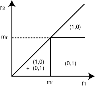
Figure 4: Monopole contributions to the superpotential for $U(3)$ gauge group with one quark and $m_{c}=0$.

This structure that we arrived at by analyzing the fermionic zero modes in the monopole background can also be seen from the one loop expression for $\phi$ (2.21) in the weak coupling region $|r_{i}-r_{j}|>>e^{2}$. Alternatively, the expression for $\phi_{i}$ can be computed as

$$\phi_{i}=\int g_{ii}dr_{i}+i\sigma_{i}\mskip 6.0mu,$$ (4.6)

where $g_{ij}$ is the one loop metric on the Columb branch in the weak coupling regions, which can be extracted from [8]. In these regions the off diagonal terms of the metric can be neglected, and the diagonal terms take the form

$$g_{ii}=\frac{1}{4}\left(\frac{1}{e^{2}}+\frac{1}{\sqrt{(r_{i}-m_{r})^{2}+|m_{c}|^{2}}}\right)\mskip 6.0mu.$$ (4.7)

Using (4.6) and (4.7) we get for the instanton factor $\,\,{\rm e}^{-\frac{\phi_{i}-\phi_{i+1}}{e^{2}}}$

$$\,\,{\rm e}^{-\frac{\phi_{i}-\phi_{i+1}}{e^{2}}}=\,\,{\rm e}^{-\frac{r_{i}-r_{i+1}}{2e^{2}}-i(\sigma_{i}-\sigma_{i+1})}\left(\frac{(r_{i+1}-m_{r})+\sqrt{(r_{i+1}-m_{r})^{2}+|m_{c}|^{2}}}{(r_{i}-m_{r})+\sqrt{(r_{i}-m_{r})^{2}+|m_{c}|^{2}}}\right)^{\frac{1}{2}}\mskip 6.0mu.$$ (4.8)

When $m_{c}\neq 0$ the instanton factor (4.8) is non vanishing for both $i=1,2$ and indeed we get contributions to the superpotential from the fundamental monopoles of charges $(1,0)$ and $(0,1)$, as expected in this case.

When $m_{c}=0$ we have to distinguish several regions. In the regions $r_{1}<m_{r}$ or $r_{3}>m_{r}$ the instanton factor (4.8) is non vanishing for both $i=1,2$ and we get contributions to the superpotential from both the $(1,0)$ and $(0,1)$ monopoles. In the region $r_{1}>m_{r}>r_{2}$ the instanton factor $\,\,{\rm e}^{-(\phi_{1}-\phi_{2})}$ vanishes and therfore only the $(0,1)$ monopole contributes, while in the region $r_{1}>r_{2}>m_{r}>r_{3}$ the instanton factor $\,\,{\rm e}^{-(\phi_{2}-\phi_{3})}$ vanishes and only the $(1,0)$ monopole contributes. Thus, we see a complete agreement between the zero mode analysis and the one-loop expression for the instanton factors.

As is clear from the analysis and from figure 1, in the weak coupling regions a superpotential is generated everywhere except at the region $r_{1}>m_{r},r_{2}=m_{r}$. Therefore the Coulomb branch is lifted everywhere except for that region. Classically, there is a Higgs branch emanating from this region. Since the instanton factors corresponding to the fundamental monopole vanish at this region one might expect no non-perturbatively generated superpotential on the Higgs branch. However, the zero mode analysis fails in this region. Far out in the Higgs branch the theory contains a gauge theory of the unbroken $U(2)$ gauge group with no matter, which we know has no supersymmetric vauca. Therefore, the Higgs branch is lifted, due to charge $(1,1)$ monopoles, which are the fundamental monopoles for the unbroken $U(2)$. We expect the same monopoles to also lift the root of the Higgs branch.

Summarizing the structure of the moduli space of vacua at weak coupling: The superpotential of the theory is given by (4.3) with the instanton factors of (4.8). At the classical level we have both Coulomb and Higgs branches, while at the quantum level both the Coulomb and the Higgs branches are lifted.

Note that the diagonal $r_{1}=r_{2}$ in figure 4 corresponds to the strong coupling region of the theory where the instanton calculus is not reliable and therefore the methods that we use in order to study the moduli space of vacua are not valid. However, as discussed previously, we can extrapolate the results to these region using holomorphy and global symmetries provided that the Kähler potential does not develop extra singularities, and conclude that all branches remain lifted.

4.1.3 The Two-Flavor Case $N_{f}=2$

The analysis of the theory with two quarks is similar to that of the single quark case. An interesting case is when the complex mass parameters of the two quarks vanish and we get four extra fermionic zero modes. Consider the region $r_{1}>m_{r}^{1},m_{r}^{2}>r_{2}>r_{3}$. The index formula for the fermionic zero modes in the background of a charge $(n_{1},n_{2})$ monopole reads

$$2(n_{1}+n_{2})-4n_{1}=2\mskip 6.0mu.$$ (4.9)

This suggests that in this region all monopoles of charges $(n,n+1)$ are allowed to contribute to the superpotential. However, the other selection rule (2.24) shows that $n=0$ and that only the fundamental monopole of charge $(0,1)$ contributes to the superpotential. In order to show that from field theory we can derive, as in the single flavor case, the instanton factor for the two flavor case using (4.6) and the expression for the one loop metric. We get

$$\,\,{\rm e}^{-\frac{\phi_{i}-\phi_{i+1}}{e^{2}}}=\,\,{\rm e}^{-\frac{r_{i}-r_{i+1}}{2e^{2}}-i(\sigma_{i}-\sigma_{i+1})}\left(\prod_{a=1}^{2}\frac{(r_{i+1}-m_{r}^{a})+\sqrt{(r_{i+1}-m_{r}^{a})^{2}+|m_{c}^{a}|^{2}}}{(r_{i}-m_{r}^{a})+\sqrt{(r_{i}-m_{r}^{a})^{2}+|m_{c}^{a}|^{2}}}\right)^{\frac{1}{2}}\mskip 6.0mu.$$ (4.10)

Using (4.10) in the region $r_{1}>m_{r}^{1},m_{r}^{2}>r_{2}>r_{3}$, we see that the instanton factors corresponding to monopoles of charges $(n,n+1)$ vanish unless $n=0$.

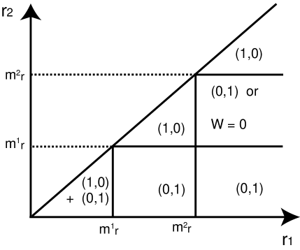
Figure 5: Monopole contributions to the superpotential for $U(3)$ gauge group with two quarks and $m_{c}=0$.

Performing the zero modes analysis as for the single flavor case we get the different monopole contributions to the superpotential as depicted in figure 5. Note that in the region $r_{1}>m_{r}^{2}>r_{2}>m_{r}^{1}$ there exist two possibilities depending on $r_{3}$. When $r_{3}<m_{r}^{1}$ there is no generation of a superpotential on the Coulomb branch by instantons. When $r_{3}>m_{r}^{1}$ the monopole with charge vector $(0,1)$ contributes and a superpotential is generated. Classically, there are Higgs branches emanating from the lines $r_{1}=m_{r}^{1}$, $r_{1}=m_{r}^{2}$, $r_{2}=m_{r}^{1}$ and $r_{2}=m_{r}^{2}$. All Higgs branches are lifted except the ones emanating from the intervals that border $W=0$ in figure 5. The Higgs branches with a non-trivial instanton factor are trivially lifted. To analyze the ones with vanishing instanton factor one can go far out on the Higgs branch and consider whether the effective field theory there has supersymmetric vacua or not.

Summarizing the quantum picture: The superpotential of the theory is given by (4.3) with the instanton factors of (4.10). Most of the Coulomb branch is lifted. In the region $r_{1}>m_{r}^{2}>r_{2}>m_{r}^{1}$ with $r_{3}<m_{r}^{1}$ there is no generation of a superpotential on the Coulomb branch by instantons and there is a quantum flat direction. Higgs branches emanate from the regions $r_{1}>m_{r}^{2},r_{2}=m_{r}^{1}$, $r_{1}>m_{r}^{2},r_{2}=m_{r}^{2}$ and $r_{1}=m_{r}^{2},m_{r}^{2}>r_{2}>m_{r}^{1}$. In the picture of [15], these Higgs branches merge with the Coulomb branch.

4.1.4 The Multi-Flavor Case

For general $N_{f}$ we have to distinguish more regions. When the complex mass parameter $m_{c}^{a}$ of the $a$’th quark is different than zero the two extra zero modes that exist when the quark was massless are lifted. This case is then reduces to the situation with $N_{f}-1$ flavors. A monopole with charge $(1,0)$ contributes only if none of the real mass parameters is in the interval $(r_{1},r_{2})$ while a monopole with charge $(0,1)$ contributes only if none of the real mass parameters is in the interval $(r_{2},r_{3})$. Again this structure can be seen from the expression for the instanton factor

$$\,\,{\rm e}^{-(\phi_{i}-\phi_{i+1})}=\,\,{\rm e}^{-\frac{r_{i}-r_{i+1}}{2e^{2}}-i(\sigma_{i}-\sigma_{i+1})}\left(\prod_{a=1}^{N_{f}}\frac{(r_{i+1}-m_{r}^{a})+\sqrt{(r_{i+1}-m_{r}^{a})^{2}+|m_{c}^{a}|^{2}}}{(r_{i}-m_{r}^{a})+\sqrt{(r_{i}-m_{r}^{a})^{2}+|m_{c}^{a}|^{2}}}\right)^{\frac{1}{2}}\mskip 6.0mu.$$ (4.11)

In analogy to figure 4 and figure 5, we summmarize here the monopole contributions to the superpotential in the different regions on the Coulomb branch by

$$\sum_{i=1}^{2}\prod_{a,m_{c}^{a}\neq 0}^{N_{f}}\Theta((r_{i}-m_{r}^{a})(r_{i+1}-m_{r}^{a}))R_{i}\mskip 6.0mu,$$ (4.12)

where $\Theta$ is the step function, and $R_{i}$ are the charge vectors of the fundamental monopoles, $R_{1}=(1,0),R_{2}=(0,1)$.

Summarizing the quantum picture: The superpotential of the theory is given by (4.3) with the instanton factors of (4.11). Most of the Coulomb branch is lifted. There are regions in the Coulomb branch where a superpotential is not generated, as can be seen from (4.12). In addition, there are regions where we pass between zero and non-zero superpotentials, from which Higgs branches emanate. In case some of the real masses are equal, there will also be a Higgs branch if we pass a line where more than one quark becomes massless, but only if no monopole contributes to both sides of the region it separates. These lines may correspond to non-trivial $N=2$ superconformal field theories.

4.2 $U(N_{c})$ Gauge Group

The analysis for general $N_{c}$ follows the same lines as that of $N_{c}=3$ in the previous section.

4.2.1 Pure Yang-Mills Theory

The index formula for the fermionic zero modes in the background of a monopole with charge vector $(n_{1},n_{2},...,n_{N_{c}-1})$ takes the form

$$2\sum_{i=1}^{N_{c}-1}n_{i}=2\mskip 6.0mu.$$ (4.13)

Therefore only the fundamental monopoles with charge vectors $R_{i}=(0,...,1...,0)$ (a $1$ in the $i$’th entry) contribute to the superpotential. The corresponding instanton terms are $\,\,{\rm e}^{-(\phi_{i}-\phi_{i+1})}$. The superpotential reads

$$W=\sum_{i=1}^{N_{c}-1}\,\,{\rm e}^{-(\phi_{i}-\phi_{i+1})}\mskip 6.0mu.$$ (4.14)

This form of the superpotential has been derived by considering M-theory on a 4-fold in [3] and using open D-string instantons in [5]. Here we get the same result from a field theory viewpoint. We thus see that in the weak coupling regions the Coulomb branch is completely lifted at the quantum level.

4.2.2 The Multi-Flavor Case

It is now clear how to generalize to $U(N_{c})$ with $N_{f}$ flavors. When the complex mass parameter $m_{c}^{a}$ of the $a$’th quark is different than zero the two extra zero modes that exist when the quark was massless are lifted. This case then reduces to the case with $N_{f}-1$ flavors. A monopole with charge vector $R_{i}=(0,...,1...,0)$ contributes only if none of the real mass parameters is in the region $(r_{i},r_{i+1})$.

Performing the zero modes analysis we see that the monopole contributions to the superpotential in the different regions of the Coulomb branch can be summarized by

$$\sum_{i=1}^{N_{c}-1}\prod_{a,m_{c}^{a}\neq 0}^{N_{f}}\Theta((r_{i}-m_{r}^{a})(r_{i+1}-m_{r}^{a}))R_{i}\mskip 6.0mu.$$ (4.15)

As in the previous cases, the structure of monopole contributions to the superpotential (4.15) can be seen from the one loop expression for $\phi_{i}$ (4.11). For $N_{f}<N_{c}-1$ the Coulomb branch is lifted completely, by simple zero-mode analysis. Classically, there are Higgs branches whenever a certain number of quarks, say $p$, become massless. However, far out on the Higgs branch the theory looks like an $N_{c}-1$ gauge theory with $p-1$ flavors, and by induction one sees that in the quantum theory all Higgs branches are lifted as well. For $N_{f}\geq N_{c}-1$, there can be Coulomb and Higgs branches that remain in the quantum theory. Regions in the classical Coulomb branch where a superpotential is not generated can be read off from (4.15). The conditions for a Higgs branch to emanate are similar to those discussed at the end of section 4.1.4.

4.3 $SU(N_{c})$ Gauge Group

The analysis for $SU(N_{c})$ gauge groups is similar to that of the $U(N_{c})$ case. The difference is that now the coordinates $\{r_{i}\}$ are subject to the restriction $\sum_{i=1}^{N_{c}}r_{i}=0$. The metric that we have to integrate in order to get the expression for the instanton factors is that of $SU(N_{c})$ which is obtained from that of the $U(N_{c})$ metric by restricting to the $SU(N_{c})$ part. Alternatively, we can use formula (2.21). In order to compare the $SU(N_{c})$ case to that of $U(N_{c})$ which we studied in detail in the previous section consider the region $r_{1}>r_{2}>...>r_{N_{c}}=-\sum_{i=1}^{N_{c}-1}r_{i}$.

The difference between the $U(N_{c})$ and $SU(N_{c})$ cases is that while for $U(N_{c})$ we can take all $\{r_{i}\}$ to be positive this cannot be done for $SU(N_{c})$. This implies, for instance, that it is not possible in this region for $SU(N_{c})$ to have $r_{N_{c}}>m_{r}^{a}$ if $m_{r}^{a}>0$ where $m_{r}^{a}$ is the real mass parameter of the $a$’th quark. Therefore such ranges of parameters in which there are instanton terms contributing to the superpotential are excluded in the $SU(N_{c})$ case. In order to illustrate this consider for instance the $SU(3)$ with two flavors case. In figure 5 we noted that for $U(3)$ with two flavors in the region $r_{1}>m_{r}^{2}>r_{2}>m_{r}^{1}$ there were two possibilities depending on $r_{3}$. When $r_{3}<m_{r}^{1}$ there was no generation of a superpotential on the Coulomb branch by instantons. When $r_{3}>m_{r}^{1}$ the monopole with charge vector $(0,1)$ contributed and a superpotential was generated. This does not depend whether $m_{r}^{1}$ is positive or negative. Since for $SU(3)$ the case $r_{3}>m_{r}^{1}>0$ is excluded, there is only one possibility which is that the superpotential vanishes.

The superpotential for gauge group $SU(N_{c})$ with $N_{f}$ flavors is given by (4.14) with the instanton factors derived from (2.21). The instanton factors are identical to those in (4.11) for $i\neq N_{c}-1$, while for $i=N_{c}-1$ we get

$$\,\,{\rm e}^{-(\phi_{N_{c}-1}-\phi_{N_{c}})}=\,\,{\rm e}^{-\frac{r_{N_{c}-1}+\sum_{i=1}^{N_{c}-1}r_{i}}{2e^{2}}+i(\sigma_{N_{c}-1}+\sum_{i=1}^{N_{c}-1}\sigma_{i})}\times$$

$$\left(\prod_{a=1}^{N_{f}}\frac{\left(-\sum_{i=1}^{N_{c}-1}r_{i}-m_{r}^{a}+\sqrt{(-\sum_{i=1}^{N_{c}-1}r_{i}-m_{r}^{a})^{2}+|m_{c}^{a}|^{2}}\right)^{N_{c}}}{\left(r_{N_{c}-1}-m_{r}^{a}+\sqrt{(r_{N_{c}-1}-m_{r}^{a})^{2}+|m_{c}^{a}|^{2}}\right)\prod_{i=1}^{N_{c}-1}\left(r_{i}-m_{r}^{a}+\sqrt{(r_{i}-m_{r}^{a})^{2}+|m_{c}^{a}|^{2}}\right)}\right)^{\frac{1}{2}}\mskip 6.0mu.$$

4.4 D-brane picture

A useful alternative viewpoint on the above results is to realize the gauge theories in string theory using intersecting branes. The $N=2$ gauge theories in three dimensions can be realized on the worldvolume of a D3 brane [5] following the construction of [10, 11]. In order to realize an $N=2$ gauge theory with $U(N_{c})$ gauge group and $N_{f}$ flavors, one uses NS and NS^′ 5-branes with worldvolume coordinates $(x^{0}x^{1}x^{2}x^{3}x^{4}x^{5})$ and $(x^{0}x^{1}x^{2}x^{3}x^{8}x^{9})$ respectively, $N_{f}$ D5 branes with worldvolume coordinates $(x^{0}x^{1}x^{2}x^{7}x^{8}x^{9})$ and $N_{c}$ D3 branes with worldvolume coordinates $(x^{0}x^{1}x^{2}x^{6})$. Instanton corrections to the superpotential of the three dimensional gauge theory in the $(x^{0}x^{1}x^{2})$-direction arise from open D-string instantons corresponding to D-strings stretching between D3 branes. In [5] the superpotential for $N=2$ $U(N_{c})$ Yang-Mills theory has been derived using these open D-string instantons.

Here we want to include matter in the brane framework. Matter multiplets in this picture arise from the open strings stretching between the D5 branes and the D3 branes. We already saw in the field theory analysis that quarks can introduce extra fermionic zero modes. In the brane picture these zero modes are localized at the intersection points between the D5 branes and the open D-string worldsheet, and arise from the open fundamental strings stretching between the D5 brane and the D-string worldsheet. Each D5 brane intersecting a D-string worlsheet gives rise in this way to two fermionic zero modes. These two fermionic zero modes are the same as the ones we get from one flavor in the field theory description when the complex mass vanishes, $m_{c}=0$.

The region in the Coulomb branch where we should take these zero modes into account depends on the point of intersection with the D5 brane. In figure 4 we see a configuration where the D5 brane intersects the D-string worldsheet in the region between $r_{i}$ and $r_{i+1}$. Since the position of the D5 brane in the $x^{3}$ direction corresponds to the real mass parameter of the corresponding matter multiplet [5], this corresponds to the region $r_{i}>m_{r}>r_{i+1}$ in the analysis of the previous sections. Thus, the term $\,\,{\rm e}^{-\frac{\phi_{i}-\phi_{i+1}}{e^{2}}}$ will not contribute to the superpotential in this case, while the other instanton factors will. It is easy to see that the fermionic zero modes analysis that we make in the field theory framework is identical to that in the branes language. The dictionary between the field theory and the brane picture is that the location of the extra fermionic zero modes coming from the D5 brane intersecting the D-string worlsheet correspond to the location of the real mass parameters in the different $\{r_{i}\}$ regions.

The complex mass parameter of a quark is represented in the brane picture by the position of the corresponding D5 brane in $(x^{4},x^{5})$. Thus, setting $m_{c}\neq 0$ implies in the brane picture that the D5 brane does not intersect the D-string worlsheet and therefore the two extra fermionic zero modes which were localized at the intersetion point do not exist. This provides further evidence (besides the consideration of the limit $m_{c}\rightarrow\infty$) for our claim that there is no fermion zero mode from the matter chiral multiplet in the case $m_{c}\neq 0$.

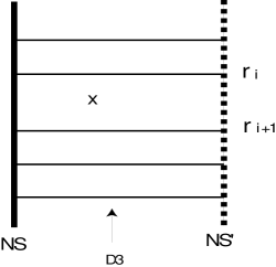
Figure 6: D-brane picture.

5 General non-abelian gauge theories

In the previous sections we have shown that for gauge groups $U(N_{c})$ and $SU(N_{c})$ with matter in the fundamental representation the non-perturbatively generated superpotential on the Coulomb branch is, at weak coupling, always of the form

$$W=\sum_{i}\,\,{\rm e}^{-\alpha_{i}\cdot\Phi}$$ (5.1)

where the sum is over the simple roots of the Lie algebra, and the result applies to the Weyl chamber where $\alpha_{i}\cdot<\Phi>>0$. In this section we will argue that this result is in fact valid for any gauge theory with arbitrary matter. To do this, we will again examine the behavior of $W$ as we send the complex masses $m_{c}\rightarrow 0$, and verify that whether $W$ vanishes or not is precisely in agreement with the Callias index theorem.

Consider a quark transforming under a representation $R$ of the gauge group, with weights $w_{p}$, real mass $m_{r}$ and complex mass $m_{c}$. According to the general result in (2.21) an exponential $\exp(-g\cdot\Phi)$, with $g$ an arbitrary magnetic charge vector, contains, due to this quark, a factor

$$\,\,{\rm e}^{-g\cdot\Phi}\sim\,\,{\rm e}^{-g\cdot(\frac{r}{2e^{2}}+i\sigma)}\prod_{p}\left[(w_{p}\cdot r-m_{r})+\sqrt{(w_{p}\cdot r-m_{r})^{2}+|m_{c}|^{2}}\right]^{-g\cdot w_{p}/2}.$$ (5.2)

As we send $|m_{c}|\rightarrow 0$, the exponential behaves as

$$\,\,{\rm e}^{-g\cdot\Phi} \sim \prod_{p}\left[(w_{p}\cdot r-m_{r})^{{\rm sign}(w_{p}\cdot r-m_{r})}|m_{c}|^{1-{\rm sign}(w_{p}\cdot r-m_{r})}\right]^{-g\cdot w_{p}/2}$$ (5.3)

$$\sim |m_{c}|^{N/2}$$

where

$$N=\sum_{p}\frac{(w_{p}\cdot r-m_{r})}{|w_{p}\cdot r-m_{r}|}(w_{p}\cdot g).$$ (5.4)

According to the results in the appendix, $N$ is precisely equal to the number of zero modes of the fermions of the quark multiplet in a monopole background with charge $g$ and scalar field vev equal to $r$. In hindsight, this is what we would expect. The one-loop corrections in $\Phi$ come from a one-loop determinant and are proportional to the product of the masses of all massive particles that are integrated out. By introducing a complex mass $m_{c}$ we give a mass proportional to $m_{c}$ to the fermion zero modes. As we take $m_{c}\rightarrow 0$, the one-loop determinant vanishes as $|m_{c}|^{N/2}$, where $N$ is the number of zero modes.

In order to have a finite contribution to the superpotential as we send all $|m_{c}|$ to zero, we need that there are no zero modes for the quarks at all in that particular monopole background. This is in complete agreement with the index theory calculation from which we obtained that if $m_{c}=0$ only monopoles that satisfy

$$2\sum_{i=1}^{{\rm rank}\,G}n_{i}\pm N=2$$ (5.5)

can contribute. This identity can only be true in a background corresponding to a fundamental monopole. These are obtained by embedding the standard $SU(2)$ monopole in an $SU(2)$ subgroup of the gauge group corresponding to a simple root. They give rise to the superpotential in (5.1), and we conclude that this is the only possible consistent superpotential.

To summarize, the superpotential on the Coulomb branch of $N=2$ gauge theory in three dimensions has the form (5.1), where $\Phi$ is given by (5.2) in the one-loop approximation.

Appendix

A Callias index

One of the main tools in the analysis in the paper was to use the number of fermionic zero modes of matter multiplets in the background of a monopole. We have seen how the number of zero modes naturally appears in one-loop calculations. In his appendix we want to show how one computes the number of zero modes using the Callias index theorem. We consider the case where we are on a point in the Coulomb branch were the gauge symmetry is maximally broken and there are no massless matter fields. If either of these two conditions is not satisfied, there is no general result regarding the number of zero modes, although some special cases, like spherically symmetric monopoles [12], can still be treated.

The bosonic part of a pure $N=2$ gauge theory in three dimensions is described by (taking $e=1$)

$$S=\int d^{3}x{\rm Tr}(\frac{1}{4}F_{ij}F^{ij}+\frac{1}{2}(D_{i}\varphi)^{2}).$$ (A.1)

where $\varphi$ is a scalar field transforming under the adjoint representation. Let $\varphi_{0}$ denote its vacuum expectation value. By assumption, it is such that it breaks the gauge group completely to its maximal abelian subgroup, and in addition all matter fields should be massive. We can rewrite the action (A.1) as

$$S=\int{\rm Tr}(\frac{1}{4}(F+\ast D\varphi)\wedge\ast(F+\ast D\varphi)+\frac{1}{4}(F-\ast D\varphi)\wedge\ast(F-\ast D\varphi)).$$ (A.2)

BPS monopoles are field configurations satisfying $F=\ast D\varphi$. For such configurations, the action in (A.2) is equal to $S=\int{\rm Tr}(F\wedge D\varphi)=\int d{\rm Tr}((F\varphi))$. This can be rewritten as an integral over a two-sphere at infinity of ${\rm Tr}(F\varphi)$. For large radius, and in a fixed direction, $F$ behaves as $(\ast F)_{i}\sim\frac{r_{i}}{r^{3}}g_{0}$, and $\varphi$ is equal to $\varphi_{0}$, so that the action for a BPS monopole configuration is $S={\rm Tr}(\varphi_{0}g_{0})$. Since $[F_{ij},\varphi]=D_{i}(D_{j}\varphi)-D_{j}(D_{i}\varphi)$ vanishes at large distances, we can simultaneously diagonalize $\varphi_{0}$ and $g_{0}$, and assume both have values in the Cartan subalgebra. Furthermore, the quantization condition for the magnetic field says that $\exp(2\pi g_{0})$ should be the identity element in the group, and therefore $g_{0}$ should be an integral linear combination of the dual simple roots of the group under consideration,

$$g_{0}=\sum n_{i}\alpha_{i}^{\ast}.$$ (A.3)

Now, consider some quark transforming in a representation $R$ of the group $G$. What we are interested in is the number of zero modes of the Dirac operator

$$D=\hbox to0.0pt{\hbox{$\mskip 3.0mu/$}\hss}D+\varphi$$ (A.4)

acting on spinors in the representation $R$. In case $\varphi$ has no zero eigenvalues in the representation $R$ (i.e. there is no massless matter), the Callias index theorem [14] can be used to compute the index of the Dirac operator. The theorem states that the index is proportional to the integral over a two-sphere at infinity of the two-form $UdUdU$, where $U=\varphi/|\varphi|$. However, for gauge groups larger than $SU(2)$ this is a very complicated calculation, and it will be easier to follow the calculation in [12, 13].

One may now compute that (using gamma matrices $\gamma_{i}=\sigma_{i}$)

$$D^{\dagger}D=-\hbox to0.0pt{\hbox{$\mskip 3.0mu/$}\hss}D\hbox to0.0pt{\hbox{$\mskip 3.0mu/$}\hss}D-\hbox to0.0pt{\hbox{$\mskip 3.0mu/$}\hss}D\varphi+\varphi^{2}=-D_{i}D_{i}+i(-(\ast F)_{k}-D_{k}\varphi)\sigma_{k}+\varphi^{2}=-D_{i}D_{i}-2\hbox to0.0pt{\hbox{$\mskip 3.0mu/$}\hss}D\varphi+\varphi^{2}$$ (A.5)

and

$$DD^{\dagger}=-\hbox to0.0pt{\hbox{$\mskip 3.0mu/$}\hss}D\hbox to0.0pt{\hbox{$\mskip 3.0mu/$}\hss}D+\hbox to0.0pt{\hbox{$\mskip 3.0mu/$}\hss}D\varphi+\varphi^{2}=-D_{i}D_{i}+i(-(\ast F)_{k}+D_{k}\varphi)\sigma_{k}+\varphi^{2}=-D_{i}D_{i}+\varphi^{2}$$ (A.6)

By hermiticity of $\varphi$, the second operator is positive definite, showing that the number of zero modes can be written as

$$N=\lim_{M^{2}\rightarrow 0}{\rm Tr}\left(\frac{M^{2}}{D^{\dagger}D+M^{2}}\right)-{\rm Tr}\left(\frac{M^{2}}{DD^{\dagger}+M^{2}}\right).$$ (A.7)

The normalizable zero modes of $D$ contribute $1$ to $N$. However, there can be a problem with (A.7) if the continuous spectrum has a singular behavior at zero, in which case there can be additional contributions to $N$ [12, 13]. In the case at hand, the long range behavior of $\varphi$ and $A_{i}$ in a fixed direction is

$$\varphi=\varphi_{0}-\frac{1}{4\pi r}g_{0}+{\cal O}(\frac{1}{r^{2}}),A_{i}=\omega_{i}g_{0}+{\cal O}(\frac{1}{r^{2}}),$$ (A.8)

where $\omega$ is the standard Dirac monopole of unit charge on $S^{2}$. Consider a fermion corresponding to a vector in the representation $R$ with weight $w$. If $w\cdot\varphi_{0}\neq 0$, the fermion decays exponentially if it has an eigenvalue close to zero, and there are no problems with the continuous spectrum. However, if $w\cdot\varphi_{0}=0$, the fermion can see an effective $1/r^{2}$ potential due to the terms of order $1/r$ in $\varphi$ and $A_{i}$. In such a potential, the spectrum can be singular, leading to an incorrect result for the number of zero modes if one uses (A.7). However, if in addition $w\cdot g_{0}=0$, the fermion does not see the $1/r$ terms and again there is no problem with the continuous spectrum. To summarize, the calculation of the number of zero modes using (A.7) is reliable if for all weights (i) $w\cdot\varphi_{0}\neq 0$ or (ii) $w\cdot\varphi_{0}=w\cdot g_{0}=0$.

To continue, we introduce Dirac matrices

$$\gamma_{i}=\left(\begin{array}[]{cc}0&i\sigma_{i}\\ -i\sigma_{i}&0\end{array}\right),\quad\gamma_{4}=\left(\begin{array}[]{cc}0&1\\ 1&0\end{array}\right),\quad\gamma_{5}=\left(\begin{array}[]{cc}1&0\\ 0&-1\end{array}\right).$$ (A.9)

and the operator ${\cal D}=\gamma_{i}D_{i}-i\gamma_{4}\varphi$. This is the Dirac operator in the four-dimensional $N=1$ theory whose dimensional reduction yields the $d=3,N=2$ theory under consideration. Using these gamma matrices, we can rewrite

$$N=\lim_{M^{2}\rightarrow 0}{\rm Tr}\left(\gamma_{5}\frac{M^{2}}{-{\cal D}^{2}+M^{2}}\right)$$ (A.10)

Next, we observe that we can write

$$N=\int d^{3}x\partial_{i}J_{i}=\int_{S^{2}_{\infty}}\hat{r}_{i}J_{i}d^{2}x$$ (A.11)

where

$$J_{i}=\frac{-1}{2}{\rm Tr}<x|\gamma_{5}\gamma_{i}{\cal D}\frac{1}{-{\cal D}^{2}+M^{2}}|x>,$$ (A.12)

and $\hat{r}_{i}$ is a unit vector on the two-sphere. We can further manipulate this expressions using the fact that

$$-{\cal D}^{2}=-D_{j}^{2}+\varphi^{2}+M^{2}+G$$ (A.13)

where $G$ is

$$G=\left(\begin{array}[]{cc}-2\hbox to0.0pt{\hbox{$\mskip 3.0mu/$}\hss}D\varphi&0\\ 0&0\end{array}\right).$$ (A.14)

and $G$ decays as $1/r^{2}$ for large $r$. If we now make an expansion of $(-{\cal D}^{2}+M^{2})^{-1}$ as a power series in $G$, then only the zeroeth and first order terms in $G$ can contribute to (A.11), the others decay too fast for that. The term independent of $G$ contains ${\rm Tr}(\gamma_{5}\gamma_{i}\gamma_{\mu})$, $\mu=1\ldots 4$, which vanishes, the term linear in $G$ contains the trace over gamma matrices ${\rm Tr}(\gamma_{5}\gamma_{i}\gamma_{\mu}G)$. If $\mu\neq 4$ one gets a term proportional to $\epsilon_{ijk}\hat{r}_{i}\hat{r}_{j}$, which vanishes. Therefore, the only relevant term remaining is, at large $r$,

$$J_{i}\sim\frac{\hat{r}_{i}}{r^{2}}{\rm Tr}<x|\varphi_{0}\frac{1}{-D_{j}^{2}+\varphi_{0}^{2}+M^{2}}g_{0}\frac{1}{-D_{j}^{2}+\varphi_{0}^{2}+M^{2}}|x>$$ (A.15)

The operator we trace is diagonal if we choose the weight basis for $R$, as both $\varphi_{0}$ and $g_{0}$ can be chosen to lie in the Cartan subalgebra. This yields

$$J_{i}\sim\frac{\hat{r}_{i}}{r^{2}}\sum_{w}(w\cdot\varphi_{0})(w\cdot g_{0})<x|\frac{1}{(-D_{j}^{2}+(w\cdot\varphi_{0})^{2}+M^{2})^{2}}|x>$$ (A.16)

The last factor is easily worked out in momentum space. Putting everything and the correct normalizations together we finally obtain

$$N=\lim_{M^{2}\rightarrow 0}\sum_{w}\frac{(w\cdot\varphi_{0})(w\cdot g_{0})}{((w\cdot\varphi_{0})^{2}+M^{2})^{1/2}}$$ (A.17)

or equivalently

$$N=\frac{1}{2}\sum_{w,(w\cdot\varphi_{0})\neq 0}({\rm sign}(w\cdot\varphi_{0}))(w\cdot g_{0}).$$ (A.18)

This result can easily be extended to the case where there is a real mass $m$ for the fermions, leading to the result

$$N=\frac{1}{2}\sum_{w,(w\cdot\varphi_{0})\neq m}({\rm sign}((w\cdot\varphi_{0})-m))(w\cdot g_{0}).$$ (A.19)

As an example, consider a fermion in the adjoint representation of SU(k), and take $\varphi_{0}={\rm diag}(\varphi_{1},\ldots,\varphi_{k})$, with $\varphi_{i}>\varphi_{i+1}$, in which case $g_{0}={\rm diag}(n_{1},n_{2}-n_{1},\ldots,-n_{k-1})$ with the $n_{i}$ nonnegative. The nonzero weights have one entry $+1$ and one entry $-1$ and all others equal to zero. This yields then

$$N_{adj}=\sum_{j>l}((n_{j+1}-n_{j})-(n_{l+1}-n_{l}))=2\sum_{i}n_{i},$$ (A.20)

the known result.

Next, consider a fermion in the fundamental representation, with real mass $m$. The weights can be taken as having one entry equal to one and all others equal to zero. Let t be the index such that $\varphi_{t}-m>0>\varphi_{t+1}-m$. If there is no such index $t$, then $N=0$, otherwise

$$N_{fund}=n_{t}.$$ (A.21)

A quark multiplet contains two fermions, and has therefore $2n_{t}$ zero modes. Notice that the number of zero modes jumps as we vary the $\varphi_{i}$.

Although we have not computed the index in the presence of a complex mass, the results of the one-loop calculations strongly suggest that there are no zero modes left as soon as a complex mass parameter is turned on. It should be quite easy to verify this in the above framework as well.

References

- [1]
- [2] I. Affleck, J. Harvey and E. Witten, “Instantons and (Super-) symmetry Breaking in (2+1) Dimensions,” Nucl. Phys. B206 (1982) 413.
- [3] S. Katz and C. Vafa, “Geometric Engineering of Quantum Field Theories,” hep-th 9611090.
- [4] E. Witten, “Non-Perturbative Superpotentials in String Theory”, hep-th 9604030, Nucl. Phys. B474 (1996) 343.
- [5] J. de Boer, K. Hori, Y. Oz and Z. Yin, “Branes and Mirror Symmetry in Supersymmetric Gauge Theories in Three Dimensions,” hep-th 9702154.
- [6] N. J. Hitchin, A. Karlhede, U. Lindstrom and M. Rocek, “HyperKähler Metrics and Supesymmetry,” Comm. Math. Phys. 117 (1988) 569.
- [7] K. Intriligator and N. Seiberg, “Mirror Symmetry in Three Dimensional Gauge Theories,” hep-th 9607207.
- [8] J. de Boer, K. Hori, H. Ooguri and Y. Oz, “Mirror Symmetry in Three-Dimensional Gauge Theories, Quivers and D-branes,” hep-th 9611063.
- [9] J. de Boer, K. Hori, H. Ooguri, Y. Oz and Z. Yin, “Mirror Symmetry in Three-Dimensional Gauge Theories, and D-brane Moduli Space,” hep-th 9612131.
- [10] S. Elitzur, A. Giveon and D. Kutasov, “Branes and Duality in String Theory”, hep-th/9702014.
- [11] A. Hanany and E. Witten, “Type IIB Superstrings, BPS Monopoles, And Three-Dimensional Gauge Dynamics”, hep-th/9611230.
- [12] E. Weinberg, “Fundamental Monopoles and Multi-Monopole Solutions for Arbitrary Simple Gauge Groups”, Nucl. Phys. B167 (1980) 500.
- [13] E. Weinberg, “Fundamental Monopoles in Theories with Arbitrary Symmetry Breaking”, Nucl. Phys. B203 (1982) 445.
- [14] C.J. Callias, “Index Theorems on Open Spaces,” Commun. Math. Phys. 62 (1978) 213.
- [15] O. Aharony, A. Hanany, K. Intriligator, N. Seiberg and M.J. Strassler, “Aspects of Supersymmetric Gauge Theories in Three Dimensions”, hep-th 9703110.