YANG-MILLS FLOW AND UNIFORMIZATION THEOREMS

S. P. Braham

Center for Experimental and Constructive Mathematics
Simon Fraser University
Burnaby, BC, V5A 1S6 Canada

J. Gegenberg

Department of Mathematics and Statistics
University of New Brunswick
Fredericton, NB E3B 4A3 Canada

Abstract

We consider a parabolic-like systems of differential equations involving geometrical quantities to examine uniformization theorems for two- and three-dimensional closed orientable manifolds. We find that in the two-dimensional case there is a simple gauge theoretic flow for a connection built from a Riemannian structure, and that the convergence of the flow to the fixed points is consistent with the Poincare Uniformization Theorem. We construct a similar system for the three-dimensional case. Here the connection is built from a Riemannian geometry, an SO(3) connection and two other 1-form fields which take their values in the SO(3) algebra. The flat connections include the eight homogeneous geometries relevant to the three-dimensional uniformization theorem conjectured by W. Thurston. The fixed points of the flow include, besides the flat connections (and their local deformations), non-flat solutions of the Yang-Mills equations. These latter “instanton” configurations may be relevant to the fact that generic 3-manifolds do not admit one of the homogeneous geometries, but may be decomposed into “simple 3-manifolds” which do.

UNB Technical Report 97-01

March, 1997

1 Introduction

The uniformization theorem in two dimensions is a powerful tool in geometry and topology, with applications in physics. In essence, the theorem states that the topology of a closed orientable two-dimensional manifold (a Riemann surface) determines which geometries it admits. In particular, if the manifold has handle number zero, it admits the spherical geometry and its local deformations; handle number one admits the flat geometry and its local deformations; and for handle number two or greater, the admissible geometry is that of the hyperbolic plane and its local deformations. It is important that one cannot deform any of these three geometries to obtain one of the other two.

This theorem was proved finally around the beginning of the twentieth century by H. Poincare [1]. It is a heroic proof, using the most sophisticated mathematics of the day. Unfortunately, the classical proof depended heavily on results in complex analysis, and the generalization to three or higher dimensions was not obvious. In fact, the three-dimensional analogue of this theorem was first consistently formulated only in the late 1970’s by W. Thurston and is called Thurston’s Geometrization Conjecture [2]. To date, although no counterexamples have emerged and it has been shown to hold for very large classes of manifolds, the conjecture remains unproved.

Recently, R. Hamilton and B. Chow have constructed a new proof of the two-dimensional uniformization theorem using techniques not obviously restricted to that number of dimensions [3, 4]. They consider a one parameter family of Riemannian metrics $g_{\mu\nu}$ on an $n$-dimensional smooth manifold $M_{n}$, with the “flow” governed by the Ricci curvature tensor $R_{\mu\nu}$:

$${\partial g_{\mu\nu}\over\partial t}=-2R_{\mu\nu}+{2\over n}rg_{\mu\nu}.$$ (1)

In the above $r$ is given by

$$r:=\left(\int_{M_{n}}d^{n}x\sqrt{g}\right)^{-1}\int_{M_{n}}d^{n}x\sqrt{g}R,$$ (2)

where $d^{n}x\sqrt{g}$, with $g=\det\left(g_{\mu\nu}\right)$, is the volume element on $M_{n}$. It is easy to show that (i.) $\partial r/\partial t=0$ along the flow; and (ii.) the fixed points of the flow are the “Einstein metrics”, satisfying $R_{\mu\nu}=(r/n)g_{\mu\nu}$. In two dimensions, the Einstein metrics have constant curvature, and include all homogeneous geometries; in three dimensions, the Einstein metrics include the constant curvature, but not all the homogeneous geometries; and finally, in four and higher dimensions, the Einstein metrics do not have nearly so clear a geometric significance as they do in lower dimensions.

The Hamilton/Chow proof of the uniformization theorem in two dimensions analyzes the “Ricci scalar flow”

$${\partial R\over\partial t}=\Delta R+R(R-r),$$ (3)

derived from the flow of the metric above. For the cases where $R$ is non-positive, it is fairly straightforward to show that the flow converges to the fixed points with non-positive constant curvature [3]. It took a few more years to analyze the case of $R>0$, since this involves a repulsive fixed point [4].

Isenberg and Jackson [5] examined the Ricci flow in three dimensions in order to shed light on Thurston’s Geometrization Conjecture [2]. Unlike the two-dimensional case, it is not true in three dimensions that all closed orientable manifolds admit one of the constant curvature geometries. Rather, one must first canonically decompose the given manifold $M$ into its prime pieces [6], obtained by cutting along 2-spheres and gluing 3-balls onto the cuts until one or both of pieces is homeomorphic to the 3-ball; then cutting along incompressible $T^{2}$ until the pieces are either Seifert fiber spaces or contain no embedded incompressible $T^{2}$. Denoting the resulting manifolds by $M_{i}$, so that $M=M_{1}\#M_{2}\#...$, Thurston then conjectures that the universal covers $\tilde{M}_{i}$ of each $M_{i}$ admits one and only one of the eight homogeneous geometries possible in three dimensions. See Table 1. for a list of these eight geometries.

$$\begin{array}[]{|l|l|l|}\hline\cr\mbox{Manifold}&\mbox{Isometry Group}&\mbox{Metric}\\ \hline\cr S^{3}&SO(4)&\cos^{2}{y}\,dx^{2}+dy^{2}+(dz-\sin{y}\,dx)^{2}\\ E^{3}&R^{3}\times SO(3)&dx^{2}+dy^{2}+dz^{2}\\ H^{3}&PSL(2,C)&dx^{2}+e^{2x}\left(dy^{2}+dz^{2}\right)\\ S^{2}\times E^{1}&\left(Isom(S^{2})\times Isom(E^{1})\right)^{+}&dx^{2}+dy^{2}+\sin^{2}{y}\,dz^{2}\\ H^{2}\times E^{1}&\left(Isom(H^{2})\times Isom(E^{2})\right)^{+}&dx^{2}+dy^{2}+e^{2x}dz^{2}\\ \widetilde{SL(2,R)}&Isom(H^{2})\times R&\cosh^{2}{y}\,dx^{2}+dy^{2}+(dz+\sinh{y}\,dx)^{2}\\ Nil&Isom(E^{2})\times R&dx^{2}+dy^{2}+(dz-xdy)^{2}\\ Sol&Sol\times\left(Z_{2}\right)^{2}&dx^{2}+e^{-2x}dy^{2}+e^{2x}dz^{2}\\ \hline\cr\end{array}$$

Table 1: The Eight Homogeneous Geometries

The problem with the approach of Isenberg and Jackson is that on the one hand, there does not seem to be sufficient structure in the Ricci flow to cope with the neccessity of decomposing the given manifold as above; and on the other the fixed points are the constant curvature geometries, a proper subset of the homogeneous geometries. Hence, one must first cut and paste the manifold, then flow the geometry on each piece; and one must look in general for asymptotics, rather than convergence to fixed points

What we propose here is a one-parameter family of connections whose flow converges to flat connections. In two dimensions, these flat connections are equivalent to the constant curvature geometries. This suggests the possibility of another proof of the two-dimensional uniformization theorem. What is important here is that this flow generalizes to three dimensions such that the fixed points of the flow are the eight homogeneous geometries plus certain “instanton” configurations, which describe “necks” between three-manifolds. We believe that this is a promising aproach to proving Thurston’s Geometrization Conjecture.

In Section 2., motivated by the gauge-theoretic formulation of certain two-dimensional gravity theories, we will recast the structure equations for a constant curvature Riemannian metric into the form of a flatness condition on an appropriate connection. This sets the stage for constructing a one-parameter family of connections – the Yang-Mills flow. In section 3., the properties of the Yang-Mills flow will be explicated. We will show that the fixed points of the flow are Yang-Mills connections, a subclass of which is the set of flat connections, and that the latter describe Riemannian metrics of constant curvature. In section 4., we analyze the behaviour of the flow. For the cases of spherical and flat Euclidean topologies, we may conclude that the flow converges to the fixed points. We present arguments to show that with initial conditions consistent with regular torsion-free Riemannian geometries, the flow actually converges to the fixed points associated with flat connections, and hence to constant curvature Riemannian geometries. This leads us to believe that one may prove the two-dimensional uniformization theorem using the Yang-Mills flow. In section 5., we outline a numerical integration of the Yang-Mills flow. Finally, in section 6., we will propose a generalization of the Yang-Mills flow to three dimensions. We will conclude by sketching the outline of the form that a proof of the Thurston Geometrization Conjecture, using this three-dimensional flow, might take.

2 Gauge Theory Form of 2D Gravity

One of the most fruitful areas of research in fundamental physics at the moment begins with the reformulation of Einstein’s theory of gravity – the general theory of relativity – as a gauge theory of the (complexified) rotation group SO(3). This approach, pioneered by A. Ashtekar and his collaborators [8], has resulted in some progress in constructing a quantum theory of gravity. This is in part due to the fact that the constraints in the theory become polynomial when expressed in terms of the above connection and its conjugate momentum; and this in turn has allowed for the construction of solutions of the constraints. Even more striking results have been attained by reformulating lower dimensional gravity theories as gauge theories. In particular, three-dimensional general relativity can be formulated as a Chern-Simons gauge theory [9]; and some simple two-dimensional gravity theories can be expressed as topological field theories of the so-called BF type [10, 11].

This suggests that it might be useful to examine the flow of connections constructed from the Riemannian geometry, rather than the flow of the metrics themselves. For one thing, as in the above theories of gravity, when expressed in connection form, we expect that the partial differential equations that describe the flow will be polynomial, unlike the Ricci flow, where the terms involving the curvature tensor are non-polynomial in the metric. More importantly, we note that the connection formulation of lower dimensional gravity theories are topological field theories, and provide a more direct route to the global issues that must be addressed.

The fixed points of the Ricci flow are the Einstein spaces. In two dimensions these are just the spaces which have constant curvature Riemannian metrics: $R=2k$. About ten years ago, Jackiw and Teitelboim (separately) considered the above as a toy model of gravity in two dimensions [12]. A few years later, at least three groups constructed a gauge theory formulation [10]. In this formulation, the field equations of the theory required that a certain connection over spacetime is flat; this in turn was equivalent to the existence of a constant curvature (pseudo-)Riemannian geometry on the spacetime. In the following, we will construct the connection which has this property.

We now consider Riemannian geometry in the first-order Cartan formalism. Instead of the metric tensor $g_{\mu\nu}$ we consider a frame-field $e^{a}$, a set of two 1-form fields on $M^{2}$. The indices $a,b,..=1,2$. The metric and frame-fields are related by $g_{\mu\nu}=\delta_{ab}e^{a}_{\mu}e^{b}_{\nu}$. Instead of the Christoffel symbols, we have the spin-connection $\omega^{a}{}_{b}$, also a set of 1-form fields on $M^{2}$. The spin-connection is skew-symmetric in the indices $a,b$, so in two dimensions, there is only one algebraically independent component, which we denote simply by $\omega$, defined by $\omega^{a}{}_{b}=-\omega\epsilon^{a}{}_{b}$.

We can now define a connection 1-form field $A$:

$$A:=e^{a}P_{a}+\omega J,$$ (4)

where $\{P_{a},J\}$ generate the Lie algebra:

$$\left[P_{a},P_{b}\right]=k\epsilon_{ab}J;\,\,\,\left[J,P_{a}\right]=\epsilon_{ab}\delta^{bc}P_{c},$$ (5)

with $\delta^{ab}$ the Euclidean metric. The algebra generated by $\{P_{a},J\}$ is so(3) if $k=+1$, iso(2) (the “Poincare algebra”) if $k=0$, or so(2,1) if $k=-1$. If the torsion

$$T^{a}:=de^{a}-\epsilon^{a}{}_{b}\omega\wedge e^{b}=0.$$ (6)

then the connection $A$ determines a Riemannian geometry.

The curvature 2-form corresponding to the connection $A$ is given by:

$$F(A): = dA+{1\over 2}[A,A]$$ (7)

$$= T^{a}P_{a}+\left(d\omega+{k\over 2}\epsilon_{ab}e^{a}\wedge e^{b}\right)J$$ (8)

$$= T^{a}P_{a}-{1\over 2}\left(R-2k\right)vJ.$$ (9)

In the above, $v={1\over 2}\epsilon_{ab}e^{a}\wedge e^{b}$ is the volume element on the manifold $M$ induced by the Riemannian metric.

If the connection $A$ is flat, then the curvature $F=0$, and hence

$$T^{a} = 0;$$ (10)

$$R = 2k.$$ (11)

Hence, a flat connection $A$, with algebra given by $k$, determines a Riemannian geometry with constant curvature $2k$, and vice-versa.

3 Yang-Mills Flow

In this section, we will describe a one-parameter family of connections, of the form given in the previous section.

We start with a two-dimensional manifold $M$ and an admissible Riemannian metric $\bar{g}_{\mu\nu}$ and a (not necessarily compatible) spin-connection $\bar{\omega}$. We use this structure to define the duals of form fields, e.g.

$$*\left(b_{\mu}dx^{\mu}\right):=\bar{g}^{1/2}\epsilon_{\mu\nu}\bar{g}^{\nu\sigma}b_{\sigma}dx^{\mu},$$ (12)

where $\bar{g}$ is the determinant of $\bar{g}_{\mu\nu}$. The algebra Eq.(5) is characterized by the constant $k$. This is determined from the topological structure of $M$ by the Euler number $\chi(M)$:

$$k:={\chi(M)\over\mid\chi(M)\mid},$$ (13)

if $\chi(M)\neq 0$, and by

$$k=0,$$ (14)

if $\chi(M)=0$. In fact, $\chi(M)$ can be computed from $\bar{g}_{\mu\nu}$ by

$$\chi(M)={1\over 4\pi}\int_{M}d^{2}x\sqrt{\bar{g}}\bar{g}^{\mu\nu}\bar{R}_{\mu\nu},$$ (15)

where $\bar{R}_{\mu\nu}$ is the Ricci tensor of $\bar{g}_{\mu\nu}$. The Euler number $\chi(M)$ is related to the handle number, or genus $h(M)$ of $M$ by $\chi(M)=2-2h(M)$.

We now flow the connection $A(t)$ given by

$$A(t)=e^{a}(t)P_{a}+\omega(t)J.$$ (16)

The initial values are given by

$$A(0)=\bar{e}^{a}P_{a}+\bar{\omega}J.$$ (17)

The differential equations that determine the flow are

$${\partial A\over\partial t}=-*D_{A}*F(A).$$ (18)

The dual $*$ and the Lie algebra are determined by the initial fields, as discussed above. Hence $*$ and $\partial/\partial t$ commute.

The parabolic-like structure of the flow is displayed most transparently in the equations for the flow of the curvature. Using Eq.(18) and the duality in two dimensions of 2-forms with 0-forms, we arrive at

$${\partial f\over\partial t}=\Delta_{A}f,$$ (19)

where $f:=*F(A)$ is a Lie algebra valued 0-form equivalent to the curvature; and $\Delta_{A}:=-\left(*D_{A}*D_{A}+D_{A}*D_{A}*\right)$ is the Laplacian with respect to the connection $A(t)$.

The fixed points of the flow are the Yang-Mills connections $A_{ym}$, i.e., connections which satisfy the Yang-Mills equations:

$$-*D_{A_{ym}}*F(A_{ym})=0.$$ (20)

There are two types of Yang-Mills connections. The first are flat connections, i.e. $F(A)=0$. If the $e^{a}$ are non-degenerate, these connections are equivalent to the constant curvature Riemannian geometries, as we discussed in the last section. The second type of Yang-Mills connections are “instantons,” with $F(A)\neq 0$. In this case, the structure group of the connection is reduced to a subgroup which commutes with $f:=*F$ [15].

In order to prove a two-dimensional uniformization theorem, we must establish the following:

Conjecture: From an initial connection corresponding to a sufficiently smooth non-degenerate Riemannian geometry on a 2-manifold $M$ with Euler number $\chi(M)$, the Yang-Mills flow converges to the flat connection corresponding to a Riemannian geometry with constant curvature having the same sign as $\chi(M)$.

In the following two sections we will provide analytical and numerical evidence for this conjecture.

4 Convergence of the Yang-Mills Flow: Analytical Evidence

There has been some discussion of the properties of Yang-Mills (and related) flows by mathematicians and mathematical physicists [16]. It is clear from this literature, in particular from the thesis of Rade, that the flow exists and is unique for short times, at least for the case of non-negative Euler number. Unfortunately, the situation with regard to the question of the convergence of flow as $t\to\infty$ is not clear at the moment. In the following, we will discuss the question of convergence from an analytic (but fairly heuristic) perspective. In the next section, encouraging results from numerical treatment will be presented.

The Yang-Mills flow resembles the heat equation

$${\partial\phi\over\partial t}=\Delta\phi,$$ (21)

where $\Delta$ is the Laplacian operator with respect to some Riemannian structure defined on the manifold $M$ upon which the field $\phi$ takes its values. The existence/uniqueness for short times and the convergence as $t\to\infty$ to the “average” initial data is well-known [17]. Indeed, it is easy to see that for initial data infinitesimally close to a fixed point, the Yang-Mills flow is parabolic. In general the Yang-Mills flow is polynomially non-linear.

We will now discuss the question of convergence for each of the cases $k=0$ and $k=+1$. The $k=-1$ case is the least well-understood at the moment, and is under investigation by the authors.

For the case $k=0$ the Lie algebra is ISO(2), which is a semi-direct product of the Abelian group SO(2) with the two-parameter group of translations. The Yang-Mills flow itself splits into an SO(2) piece which depends only on the $A^{2}$-component of the ISO(2) connection:

$${\partial A^{2}\over\partial t}=-*d*dA^{2}.$$ (22)

Although this is not strictly parabolic, the flow of the corresponding dual of the curvature component, $f^{2}:=*F^{2}=*dA^{2}$ is a parabolic system:

$${\partial f^{2}\over\partial t}=\bar{\Delta}f^{2},$$ (23)

where $\bar{\Delta}$ is the Laplacian with respect to the initial Riemannian geometry. Now the average of the initial curvature component,

$$\bar{F}^{2}:=\int_{M^{2}}dA^{2}=0,$$ (24)

where the last equality follows from the fact the in this case $M^{2}$ has Euler number zero. Since $f^{2}$ converges to a constant 0-form, it must converge to zero everywhere on $M_{2}$.

What we have shown is that the manifold which is topologically $T^{2}$, i.e which has Euler number 0, admits a closed 1-form. This is a sufficient condition that the manifold admits a Riemanian geometry with a compatible spin-connection with zero curvature. To see this, consider the following: Let $\omega$ be a closed 1-form. But since for $T^{2}$ the space of harmonic 1-forms is two-dimensional, there is a harmonic 1-form $\beta$ such that $\omega\wedge\beta\neq 0$. We can find a chart in which there is a function $p(x)$, such that $\partial_{\mu}p(x)=\beta_{\mu}(x)$. Now define the 1-forms $e^{0},e^{1}$ in this chart by $e^{0}(x)=p(x)\omega(x),e^{1}(x)=-dp(x)$. In the chart, the volume element $e^{0}(x)\wedge e^{1}(x)\neq 0$ by construction, and the compatibility condtion $de^{a}-\epsilon^{a}{}_{b}\omega\wedge e^{b}=0$ since $d\omega=0$.

It remains to address the question of which initial conditions, if any, determine flows which converge to the instantons, with $F(A_{\infty})\neq 0$.

In the $k=+1$ case, for which the gauge group is SO(3), we have the results of Rade [16] wherein in is proved that for compact simple gauge groups, e.g. SO(3), the Yang-Mills flow converges with respect to the Sobolev norm $H^{1}$ to a Yang-Mills connection. What remains here is the question of the instantons, as well as whether the flow converges under stronger smoothness requirements.

5 Convergence of the Yang-Mills Flow: Experimental Differential Geometry

The system of coupled partial differential equations Eq.(18) is comprised of polynomially nonlinear PDEs, and is therefore potentially quite complicated. However, the right-hand side of Eq.(18) contains second derivatives in the spatial variables and is therefore much like a diffusive system with strange convective terms. If we effectively restrict consideration to the very high frequency components of Eq.(18) by only retaining terms that contain the highest number of spatial derivatives, we find that

$$\frac{\partial A}{\partial t}\approx\delta dA,$$ (25)

where $\delta=-*d*$. The right-hand side of Eq.(25) is not the Laplacian on $M$ defined by the initial connection, which would be given by $\Delta=\delta d+d\delta$. Thus, the system does not, even in this approximation, represent an exact diffusive evolution. However, under the same conditions for which Eq.(25) is valid, we have

$$\frac{\partial f}{\partial t}\approx\Delta f,$$ (26)

which is a diffusive equation. It is therefore highly probable that high frequency spatial perturbations in the curvature and torsion induced on $M$ by $A(t)$ are rapidly damped as $t\rightarrow\infty$. We would therefore expect a breakdown of our conjectured convergence behaviour of the flow only if the low frequency modes do not have the appropriate evolution. These modes are dominated by the nonlinear coupling in Eq.(18).

It seems highly probable that such a system will not lend itself to easy analytic study. Rather, before attempting such an analysis, it seems appropriate that we should verify the conjectured behaviour as best we can. To do this, we resort to techniques of experimental mathematics, wherein we view the conjectured convergence behaviour as a hypothesis. We will seek experimental evidence for or against the hypothesis.

We can then study the following two questions:

1. Does $A$ evolve smoothly under Eq.(18) from smooth initial data?

2. Does $A$ converge to a fixed point in an appropriate space of connections over $M$?

If both questions have affirmative answers, we would also like to answer the concomitant question:

1. Does $F(A)\rightarrow 0$ as $t\rightarrow\infty$?

Should the answers to these questions turn out to be yes, for a reasonably wide set of initial conditions and topologies, we would have hope that further study of the flow method ought to be useful in understanding uniformization theorems. We might further hope that our numerical “experiments” would enable us to observe useful properties of Eq.(18) that help suggest ways to prove our conjecture. To the contrary, should we find a numerical counterexample to our conjecture, we could rapidly verify that the conjecture would be false. This is the heart of the experimental mathematics concept. Given that we conjecture Eq.(18) to be diffusive and parabolic, we must first choose a numerical method appropriate to such equations. It is then an important part of the experimental process to verify the consistency of the chosen method. The explicit forward Euler method is the most naive numerical integration method appropriate for diffusive parabolic PDEs. It is important to choose carefully. Assume for the moment that the “convection” terms were to dominate over the “diffusion” terms, producing dynamics for $A$ that are far more like hyperbolic systems. Hyperbolic PDEs are generally unstable when evolved via naive numerical methods, such as the forward Euler method. Furthermore, it would seem improbable that $A$ would converge if Eq.(18) was primarily hyperbolic in nature and if $M$ was compact.

In the Euler method, the iterated value of the connection at time $t_{n+1}>t_{n}$ is taken to be

$$A_{n+1}=A_{n}-\kappa(*D_{A}f(A_{n})),$$ (27)

where $A_{n}$ is the value of $A$ at a time $t_{n}:=t_{0}+n\kappa$, $\kappa>0$, and where $A_{i}$ is given on a mesh of discrete points approximating the manifold $M$. Such an approximation is shown in Figure 1, where an initial connection is represented on a torus. The curvature is represented by variations of the torus geometry, and the actual torus generated is only a representation of the state of $A(t)$ and $f(t)$.

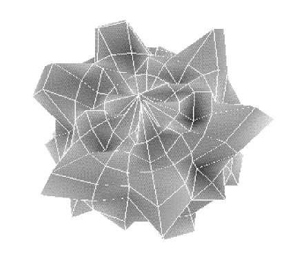
Figure 1: An initial toroidal mesh.

We wish to compare Eq.(18) to the evolution of a linear system of the form

$$\frac{\partial u}{\partial t}=Ku(t),$$ (28)

where $u$ is a quantity given on $M$, and $K$ is a linear operator acting on $u$. The corresponding forward Euler method is

$$u_{n+1}=u_{n}+\kappa Ku_{n},$$ (29)

where everything is expressed on a mesh over $M$. It is well-known that Eq.(29) fails to produce a valid approximation to the solution of the hyperbolic equation Eq.(28): the numerically produced solution undergoes rapid growth in modes that are high in spatial frequency. The approximation is bad, independently of how small we take $\kappa$ to be. Diffusive parabolic systems are different in behaviour: for $\kappa$ small enough, the numerical solution obeys Eq.(28).

In view of this comparison, part of our experiment consists of identifying whether Eq.(27) produces a stable approximation (suggesting parabolic behaviour) or an unstable one (suggesting hyperbolic behavour).

The experimental procedure is as follows: the symbolic system Maple is used to write part of the computer program, converting Eq.(27) into computer code representing evolution on an appropriate mesh with cell size $h$ and time-step $\kappa$. We then verify the stability behaviour for $\kappa$ vs. $h$. If we observe the expected stability behaviour, we can then analyse the resulting evolution to see if it is consistent with our conjecture.

Happily, Eq.(27) does indeed display, for $k=0$, the precise behaviour of a diffusive parabolic PDE. To be precise, for a toroidal rectangular mesh, the numerical stability is observed when $\kappa$ is smaller than a value that is of order $h^{2}$, for a wide range of initial conditions. One particular example of this can be seen in Figure 2.

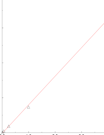
Figure 2: Stability behaviour of the forward Euler method for the flow equations. Line marks linear fit.

This is the anticipated signature of a diffusive system, whence we have verified one part of our conjecture, as discussed above. Furthermore, we obtain evidence that, for the $k=0$ case, all three of our earlier questions may be answered in the affirmative. We find that the numerical evolution of Eq.(18) under Eq.(27) produces a convergent $A_{n}$, and that $F(A_{n})\rightarrow 0$, as $n\rightarrow\infty$. This is shown in the final state of the mesh; cf. Figure 3, also drawn on top of the representative torus.

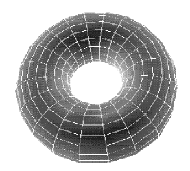
Figure 3: The final configuration, after numerical evolution.

We have therefore found support for our conjectured convergence behaviour of solutions of Eq.(18), at the experimental level, for $k=0$.

The conjecture can also be experimentally verified for the $k=1$ (spherical topology) case. In the spherical case, we construct an initial connection on a mesh with spherical topology, as shown in Figure 4. The radius from the centre in this image denotes the curvature radius at that point.

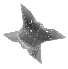
Figure 4: An initial connection for a spherical topology.

Figure 5: Final, unit sphere, result of evolution.

The flow equations can then be evolved. The connection then flows to one corresponding to a unit 2-sphere, as shown in Figure 5. We thus have experimental confirmation of the conjecture for $k=0$ and $k=1$.

It remains to verify the conjecture for $k<0$. Unfortunately, Eq.(27) is not very useful in this case. The fact that $\kappa$ must be smaller than something of order $h^{2}$ means that the equations cannot be evolved quickly when we wish to have $h$ small. For complicated topologies that arise for $k<0$ (particularly handlebodies, which do not arise in the other cases), we need many cells, and $h$ must be small. Furthermore, it becomes difficult to control the build up of numerical noise with such a naive, conditionally stable, method. For $k<0$ (and the 3-D flow described in the next section), more sophisticated techniques will be needed. These techniques will have to deal with the fact that $M$ will generally need to be covered by more than one coordinate patch, more than one gauge patch, will have complicated topology, and even more nonlinear behaviour. The best practical algorithms seem to be those using multigrid finite element methods. One of us (SPB) is currently developing such techniques.

6 The 3-D Flow

The gauge-theoretic version of a two-dimensional theory of gravity was the starting point for a new approach to proving the two-dimensional uniformization theorem. We emphasize here that we have not completely succeeded in constructing the proof; we have only demonstrated its plausibility. Neverthless, this suggests that it might be useful to examine gauge-theoretic versions of 3-D gravity theories as possible starting points for a proof of the 3-D uniformization theorem conjectured by Thurston.

Such theories are well-known. Einstein gravity (with or without a cosmological constant) can be formulated as a Chern-Simons gauge theory with gauge group ISO(3) (if the cosmological constant is zero) or SO(4) or SO(3,1) if the cosmological constant is positive or negative [9]. This suggests that we consider a flow of the form

$${\partial A\over\partial t}=*D_{A}*F(A),$$ (30)

where $A$ is the connection 1-form on some 3-manifold for some gauge group $G$. One recovers the Riemannian geometry from the connection 1-form via a relation of the form:

$$A=\omega^{a}G_{a}+e^{a}F_{a}+...,$$ (31)

where the $G_{a},F_{a}$ are generators of $G$, and the $e^{a},\omega^{a}$ can be interpreted as a frame field and spin-connection, respectively. The $...$ indicates other terms in any additional generators of the gauge group $G$. The idea is to choose the gauge group $G$ so that the flat connections (which are a subset of the fixed points of the flow) include at least the eight homogeneous geometries that occur in Thurston’s conjecture. This is not the case if one chooses one of the groups (ISO(3), etc.) relevant to Einstein gravity. The flat connections for these groups determine frame-fields $e^{a}$ and compatible spin-connections $\omega^{a}$ which have constant curvature.

There is a gauge group whose flat connections include the eight homogeneous three-dimensional geometries. The group is the “doubly inhomogenized” group IISO(3). This group is the semi-direct product of the “Poincare group” ISO(3) with its Lie algebra. It is a twelve parameter non-compact group, whose Lie algebra is

$$\left[F^{a},G^{b}\right] = {1\over 2}\epsilon^{abc}F_{c};\,\,\,\left[G^{a},G^{b}\right]={1\over 2}\epsilon^{abc}G_{c};$$ (32)

$$\left[G^{a},J^{b}\right] = {1\over 2}\epsilon^{abc}J_{c};\,\,\,\left[G^{a},K^{b}\right]={1\over 2}\epsilon^{abc}K_{c};$$ (33)

$$\left[J^{a},K^{b}\right] = {1\over 2}\epsilon^{abc}F_{c}\,\,\,.$$ (34)

The remaining brackets vanish. The $G^{a}$ generate the SO(3) subgroup, while the remaining generators $F^{a},J^{a},K^{a}$ behave like generators of translations, except that the latter two do not commute.

It was shown in [14] that the Chern-Simons functional with this gauge group is equivalent to a three-dimensional theory of gravity interacting with topological matter. This is accomplished by constructing the IISO(3) connection as follows:

$$A=\omega^{a}G_{a}+e^{a}F_{a}+B^{a}J_{a}+C^{a}K_{a}.$$ (35)

If $A$ is flat, i.e. if $F(A)=0$, then by use of the algebra Eq.(34) it follows that $\omega^{a}$ is a flat SO(3) connection, $B^{a},C^{a}$ are covariantly constant with respect to $\omega^{a}$ and $e^{a}$ satisfies:

$$D_{\omega}e^{a}+{1\over 2}\epsilon^{abc}B_{b}\wedge C_{c}=0,$$ (36)

where $D_{\omega}$ is the gauge covariant derivative with respect to the connection $\omega^{a}$.

One may now construct a spin-connection which is compatible with the frame-field $e^{a}$, and hence determines a Riemannian geometry. In particular, one can show that if the $e^{a}$ are the frame-fields for a homogeneous geometry, then there exist flat connections $\omega^{a}$ and fields $B^{a},C^{a}$ satisfying $D_{\omega}B^{a}=0,D_{\omega}C^{a}=0$ such that $e^{a}$ satifies Eq.(36). The explicit expressions are shown in Tables 2 and 3, where we have taken $\omega^{a}=0$ for simplicity.

$$\begin{array}[]{|l|l|}\hline\cr\mbox{3-manifold}&\left(e^{1},e^{2},e^{3}\right)\\ \hline\cr S^{3}&\left(\cos{y}\,dx,dy,dz-\sin{y}\,dx\right)\\ E^{3}&\left(dx,dy,dz\right)\\ H^{3}&\left(dx,e^{x}dy,e^{x}dz\right)\\ S^{2}\times E^{1}&(dx,dy,\sin{y}\,dz)\\ H^{2}\times E^{1}&\left(dx,dy,e^{x}dz\right)\\ \widetilde{SL(2,R)}&(\cosh{y}\,dx,dy,dz+\sinh{y}\,dx)\\ Nil&(dx-zdy,dy,dz)\\ Sol&\left(dx,e^{-x}dy,e^{x}dz\right)\\ \hline\cr\end{array}$$

Table 2: Frame Fields for Homogeneous Geometries

$$\begin{array}[]{|l|l|l|}\hline\cr\mbox{3-manifold}&\left(B^{1},B^{2},B^{3}\right)&\left(C_{1},C_{2},C_{3}\right)\\ \hline\cr S^{3}&\left(0,dx,0\right)&\left(d(2\sin{y}),0,d(2\cos{y})\right)\\ E^{3}&(0,0,0)&(0,0,0)\\ H^{3}&\left(d\left(2e^{x}\right),0,0\right)&(0,d(-z),dy)\\ S^{2}\times E^{1}&(d(-2\sin{y}),0,0)&(0,dz,0)\\ H^{2}\times E^{1}&\left(d\left(-2e^{x}\right),0,0\right)&(0,dz,0)\\ \widetilde{SL(2,R)}&(0,dx,0)&(d(-2\sinh{y}),0,d(2\cosh{y}))\\ Nil&(0,dy,0)&(0,0,d(-2z))\\ Sol&\left(d\left({z-y\over 2}\right),d\left(e^{x}\right),d\left(-e^{-x}\right)\right)&\left(d\left({z+y\over 2}\right),d\left(2e^{x}\right),d\left(2e^{-x}\right)\right)\\ \hline\cr\end{array}$$

Table 3: $B$ and $C$ 1-Form Fields for Homogeneous Geometries

It must be remarked here that one may perform an IISO(3) gauge transformation on the flat connection equivalent to the homogeneous geometries. The connections are still flat, of course, but in general the $e^{a}$ are no longer frame-fields for a homogeneous geometry. It is not clear at this point how general the gauge-transformed $e^{a}$ are; though it was shown in [14] that for the case of the 3-manifold topology $S^{2}\times S^{1}$, all admissible $e^{a}$ could be obtained from the “trivial” configuration $\omega^{a}=e^{a}=B^{a}=C^{a}=0$ by a gauge transformation.

If it could be shown that an arbitrary IISO(3) connection on the 3-manifold flowed to one of the flat connections, then it would follow that the 3-manifold would admit the homogeneous representative of the gauge orbit. This is what we expect of a proof of the uniformization conjecture for 3-manifolds.

In the two-dimensional Yang-Mills flow, the fixed points of the system are the Yang-Mills connections. However, it seems to be the case that regular initial conditions will flow to the appropriate subclass of flat connections. The reason for this is that in two dimensions, the non-flat Yang-Mills connections are reducible. This is not the case in three dimensions, since the duals of the curvature 2-forms are 1-forms, and hence not gauge parameters. Hence we conjecture that in three dimensions some regular connections, built from non-degenerate Riemannian metrics, will flow to instanton fixed points, not flat fixed points. This might be related to a fundamental difference between the two- and three-dimensional cases. Indeed, as we discussed in the Introduction, in contrast to the two-dimensional case, a given closed orientable 3-manifold does not in general admit a homogeneous Riemannian geometry. Thurston’s conjecture is that any 3-manifold admits a canonical decomposition into the connected sum of simple manifolds, i.e., prime manifolds which either have no incompressible embedded $T^{2}$ or are Seifert fiber spaces; and each simple manifold in turn admits one and only one of the eight homogeneous geometries. If the flow converged to fixed points which were flat connections, then in general it would have to be singular when the manifold was not simple.

However, consider the flow of the curvature as above. The fixed points are the flat connections $F(A)=0$ and the Yang-Mills instantons which satisfy $*D_{A}*F(A)=0,\,\,F(A)\neq 0$. It would be interesting to examine IISO(3) connections on 3-manifolds to see if the Yang-Mills equations have non-flat solutions when the manifold is simple. If it turns out that simple 3-manifolds admit flat solutions of the Yang-Mills equations, then the next question to examine would be the structure of 3-manifolds which consist of two simple manifolds joined by a “neck”. If Thurston’s conjecture is correct, then the following scenario should hold: the manifold-with-neck would presumably admit an instanton which was asymptotically flat at the ends of the neck. In general, non-simple 3-manifolds would not admit non-trivial flat IISO(3) connections. Work in this direction is underway by the authors.

References

- [1] H. Poincare, Acta. Math. 31, 1 (1907).
- [2] W. Thurston, The Geometry and Topology of Three Manifolds, Princeton Un. Lecture Notes, 1978.
- [3] R. Hamilton, “The Ricci Flow on Surfaces”, in Mathematics and General Relativity, ed. J. Isenberg, Contemp. Math. 71, AMS (1988).
- [4] B. Chow, J. Diff. Geom. 33, 325 (1991).
- [5] J. Isenberg and M. Jackson, J. Diff. Geom. 35, 723 (1992).
- [6] H. Kneser, Jahr. der Deutscher Math. Ver. 38, 248 (1929); J. Milnor, Am. J. Math., 84, 1 (1962).
- [7] W. Jaco and P. Shalen, Seifert fibered spaces in 3-manifolds, Mem. Am. Math. Soc., 220, AMS, Providence, RI (1980).
- [8] For a review see, A. Ashtekar, Lectures on Non-Perturbative Canonical Gravity, World Scientific, Singapore (1991).
- [9] A. Achucarro and P. Townsend, Phys. Lett. B180, 89 (1986); E. Witten, Nuc. Phys. B311, 46 (1988).
- [10] T. Fukuyama and K. Kamimura, Phys. Lett. B160, 259 (1985); K. Isler and C. Trugenberger, Phys. Rev. Lett. 63, 834 (1989); A. Chamseddine and D. Wyler, Phys. Lett. B228, 75 (1989).
- [11] D. Cangemi and R. Jackiw, Phys. Rev. Lett. 69, 233 (1992).
- [12] R. Jackiw in Quantum Theory of Gravity, ed. by S. Christensen, Adam Hilger, Bristol (1984); C. Teitelboim in Quantum Theory of Gravity, ed. by S. Christensen, Adam Hilger, Bristol (1984).
- [13] A. S. Schwarz, Lett. Math. Phys. 2, 247 (1978); M. Blau and G. Thompson, Ann. of Phys. 205, 130 (1991); G. T. Horowitz, Comm. Math. Phys. 125, 417 (1989).
- [14] S. Carlip and J. Gegenberg, Phys. Rev. D44, 424 (1991).
- [15] M.F. Atiyah and R. Bott, Topology 23, 1 (1984); E. Witten, J. Geom. Phys. 9, 303 (1992).
- [16] For our purposes, the most relevant discussion occurs in J. Rade, On the Yang-Mills Heat Equation in Two and Three Dimensions, Ph.D. thesis, Univ. of Texas at Austin, 1991. A discussion of the four-dimensional case is C.-L. Shen, in XXI International Copnference on Differential Geometric Methods in Theoretical Physics, ed. C.N. Yang, M. L. Ge and X.W. Zhou, World Scientific, Singapore, 1993. See also L.A. Sadun, Continuum Regularized Yang-Mills Theory, Ph.D. thesis, Univ. of California at Berkeley, 1987; K. Corlette, in Geometry of Group Representations, ed. W.M. Goldman and A.R. Magid, Contemporary Mathematics V. 74, American Mathematical Society, 1988.
- [17] See for example, R.S. Hamilton, Harmonic Maps of Manifolds with Boundary, Lecture Notes in Math. V. 471, Springer-Verlag, Berlin, 1975.