Nonlinear modification of quantum mechanics

Abstract

In order to prevent “unavoidable” break-down of the “peaceful coexistence” between foundations of quantum theory and relativity I propose a new type of a quantum gauge theory (superrelativity). This differs from ordinary gauge theories in the sense that the affine connection of this theory is constructed from first derivatives of the Fubini-Study metric tensor in the projective Hilbert space of the pure quantum states CP(N). That is we have not merely analogy with general relativity but this construction should presumably provide a unification of general relativity and quantum theory.

PACS numbers: 03.65 Bz, 03.65 Ca, 03.65 Pm

1 Introduction

The interesting project of the generalized nonlinear quantum mechanics of Weinberg [1] was subjected to the critical analysis [2] in the framework of probabilistic interpretation with respect to a possibility of the “faster-than-light communication” in nonlinear quantum dynamics. But now it has beeb shown [3] that a specific nonlinear scheme may be successfull in spite of this general criticism.

The general inspiration for my approach to the nonlinear version of quantum theory is as followes: Laws of non-relativistic classical physics are indifferent to any type of forces. But development of the theory of such natural type of force as electromagnetic demands the relativistic generalization of Newton’s mechanics. A new kind of spacetime symmtry arises. Ordinary quantum mechanics is indifferent to the choice of a potential, say in Schrödinger equation, as well. However in physics of elementary particles where a natural type of sub-atomic forces act, we can not be sure that equations and symmetry of the ordinary quantum theory may be concerved. In particular, ordinary quantum theory points out that general relativity (GR) is negligible for spatial distances up to the Planck scale $l_{P}=(\hbar G/c^{3})^{1/2}\sim 10^{-33}cm$. But consistency in the foundations of the quantum theory requires a“soft” spacetime structure of the GR at essentially longer length. However, for some reasons this appears to be not enough. A new framework (“superrelativity”) for the desirable generalization of the foundation of quantum theory has been proposed [4, 5, 6, 7, 8].

The equivalence principle of Einstein is based on the experimental fact that acceleration of bodies in the gravitation field is independent on masses of these bodies [9]. This situation is physically equivalent to the motion of the system of bodies in accelerated frame. We can not, of course, put the criterion of identical acceleration in the basis of geometrization of quantum physical fields. In quantum field theory the notion of “acceleration” is poor at best and ambiguous at worst because quantum particles have an internal structure. Furthermore, at a deeper level there is entanglement and even indistinguishability of “internal” and “external” degrees of freedom. Therefore in quantum regime we can not act literally as Einstein in GR but only in his spirit [4, 5, 6, 7, 8].

The notions of material point, event, and classical spacetime in both special relativity (SR) and GR are liable to lead to confusion at the quantum level. Insead of these objects we use a set of new primordial elements. Namely, they are pure quantum state, quantum transition, and quantum state space, respectively. These main elements provide a basis for a generalization of the equivalence principle in quantum area. The principle of superrelativity states as follows: The general unitary motion of pure quantum states may be locally reduced to the geodesic motion in the projective Hilbert space by the introduction of a gauge (compensation) field which arises from the local change of a functional frame in the original Hilbert state space.

We have put at the basis of our theory the fact that in all interactions of quantum (“elementary”) particles there is a conservation law of the electric charge. Then unitary group SU(N+1) takes the place of dynamical group because in the general case $g|\Psi>\neq|\Psi>$ and, of course, $g^{-1}Hg\neq H$ [10]. There is the group of isotropy $H=U(1)_{el}\times U(N)$ of a fixed pure quantum state $e^{i\gamma}|\Psi>$. That is transformations which effectively act on this ray lie in the coset $G/H=SU(N+1)/S[U(1)\times U(N)]$. It is clear that deformations of the pure quantum state are due to some physical interaction; the effect of the interaction has the geometric structure of a coset [4], i.e. the structure of the CP(N): $G/H=SU(N+1)/S[U(1)_{el}\times U(N)]=CP(N)$ [11]. This paves the way to the invariant study of the spontaneously broken unitary symmetry. This statement has a general character and does not depend on particular properties of the pure quantum state. The reason for the change of motion of material point is an existence of a force. The reason for the change of a pure quantum state is an interaction which may be modeled by unitary transformations from the coset G/H. The reaction of a material point is an acceleration. The reaction of a pure quantum state is its deformation whose geometry should be discussed now [4, 5, 8].

2 Break-down of the projective symmetry

Unitary symmetry in quantum mechanics is expanded to the projective symmetry due to arbitrary normalization of state vector [10]. But some interactions, gravity, for example, ban this degree of freedom and restore (with a reconstruction) the unitary symmetry. Furthermore, the global unitary summetry is broken down to the isotropy subgroup whose elements leave of some fixed ray of state $e^{i\gamma}|\Psi>$ intact. In order to uderstand a new type of symmetry arising here, we will discuss the infinitesimal interval in Hilbert space $\cal H\rm=C(N+1)$ which related to some linear Hermitian traceless operator $\hat{D}\in AlgSU(N+1)$. This operator creates some interval $d_{\hat{D}}l^{2}=d\Psi_{a}^{*}d\Psi^{a}=<d\Psi|d\Psi>=$ $<\Psi|\hat{D}^{+}\hat{D}|\Psi>d\epsilon^{2}$, where $\epsilon$ is real-number group parameter, and $\Psi^{a}$ are Fourier components of a decomposition of a state vector in some orthogonal basis $|\Psi>=\sum_{a=0}^{N}\Psi^{a}|a>$ where $\sum_{a=0}^{N}|\Psi^{a}|^{2}=R^{2}$. Now one can reduce the quadric to the principle axes by ansatz of “squeezing” full state covector to the vacuum form as in [7]

$$<\Psi_{0}|=R(\Psi)e^{i\omega(\Psi)}(1,0,...,0).$$ (2.1)

That is $|\Psi_{0}>=\hat{G}^{-1}|\Psi>$, where $\hat{G}=\hat{G}_{1}\hat{G}_{2}...\hat{G}_{N}$ are matrices which described in [7]. Since in the process of a “squeezing” gauge transformations from isotropy group should be accompanied by transformations from the coset $SU(N+1)/S[U(1)\times U(N)]$, in contrast to the gauge transformations of Ref. [3] one has an observable deformation of the quantum state. The gauge field is a physical evidence of this deformation due to the non-trivial topology of CP(N). Then one has

$$d_{\hat{D}}l^{2}=<\Psi_{0}|\hat{D^{\prime}}(\Psi)^{+}\hat{D^{\prime}}(\Psi)|\Psi_{0}>=R^{2}(|D^{\prime}_{00}(\Psi)|^{2}+\sum_{i=1}^{N}|D^{\prime}_{0i}(\Psi)|^{2})d\theta^{2}.$$ (2.2)

The first term is interval along the subalgebra of the isotropy group of the vector $|\Psi_{0}>$ and the second one is interval in the tangent space to the coset itself. One-parameter tranformation from the coset is a geodesic flow. For the covector (2.1) the geodesic flow is generated by the operator

$$\hat{B}=\left(\matrix{0&f^{1*}&f^{2*}&.&.&.&f^{N-1*}\cr f^{1}&0&0&.&.&.&0\cr f^{2}&0&0&.&.&.&0\cr.&.&.&.&.&.&.\cr.&.&.&.&.&.&.\cr.&.&.&.&.&.&.\cr f^{N-1}&0&0&.&.&.&0}\right),$$ (2.3)

where $f^{i}=D^{\prime}_{0i}(\Psi)$. The flow is given by the unitary matrix $\hat{T}(\tau,g)=\exp(i\tau\hat{B})$ where $g=\sqrt{\sum_{k=1}^{N}|f^{k}|^{2}},\Theta=g\tau$ [4]. Note, elements of tangent space to the coset will be functions of state vector during the process of the “squeezing” . In that sense local (in functional space) dynamical variables arise. But invariant properties of the interval should be independent from a particular choice of the dynamical variable $\hat{D}$. The infinitezimal interval $\delta L^{2}$ in local projective coordinates may exemplify this independece. The generalized stereographic projection from the center of the sphere $\sum_{a=0}^{N}|\Psi^{a}|^{2}=R^{2}$ onto the complex hyperplane $\Pi$ give us relationships between coordinates of a point of the sphere in the original Hilbert space $\Psi^{0},...,\Psi^{a},...,\Psi^{N}$ and coordinates $\Pi^{1},...,\Pi^{i},...,\Pi^{N}$ of its projection onto the hyperplane

$$\Psi^{0}=\lambda(R,\Pi)R,\quad\Psi^{1}=\lambda(R,\Pi)\Pi^{1},\Psi^{2}=\lambda(R,\Pi)\Pi^{2},...,\Psi^{N}=\lambda(R,\Pi)\Pi^{N}$$ (2.4)

Then one has mapping $f:C(N+1)\to CP(N)$ for ($1\leq i\leq N$)

$$\Pi^{1}=R\Psi^{1}/\Psi^{0},\Pi^{2}=R\Psi^{2}/\Psi^{0},...,\Pi^{i}=R\Psi^{i}/\Psi^{0},...,\Pi^{N}=R\Psi^{N}/\Psi^{0}$$ (2.5)

and $\lambda^{2}(\sum_{i=1}^{N}|\Pi^{i}|^{2}+R^{2})=R^{2}$. The “squeezing factor” $\lambda(R,\Pi)$ one can express from this equation

$$\lambda(R,\Pi)=R(\sum_{s=1}^{N}|\Pi^{s}|^{2}+R^{2})^{-1/2}.$$ (2.6)

Hereafter we will use only finite value of indexes $0\leq a,b,...,d\leq N$ and $1\leq i,k,...,s\leq N$, remembering that in typical cases the limit $N\to\infty$ may be studied. Now we can express homogeneous coordinates $\Psi$ in local coordinates $\Pi$:

$$\Psi^{0}=R^{2}(\sum_{s=1}^{N}|\Pi^{s}|^{2}+R^{2})^{-1/2},...,\quad\Psi^{i}=\Pi^{i}R(\sum_{s=1}^{N}|\Pi^{s}|^{2}+R^{2})^{-1/2}.$$ (2.7)

It is easy to evaluate ($a=0$)

$$\frac{\partial\Psi^{0}}{\partial\Pi^{i}}=-\frac{1}{2}R^{2}\Pi^{*i}\left(\sqrt{\sum_{s=1}^{N}|\Pi^{s}|^{2}+R^{2}}\right)^{-3},c.c.$$ (2.8)

and for other components ($a\geq 1$) one has

$$\frac{\partial\Psi^{a}}{\partial\Pi^{i}} = R\left(\delta^{a}_{i}(\sum_{s=1}^{N}|\Pi^{s}|^{2}+R^{2})^{-1/2}-\frac{1}{2}\Pi^{a}\Pi^{*i}(\sum_{s=1}^{N}|\Pi^{s}|^{2}+R^{2})^{-3/2}\right),c.c.$$ (2.9)

Therefore one can express infinitezimal invariant interval in the original Hilbert space as followes

$$\delta L^{2}=\delta_{ab}\delta\Psi^{a}\delta\Psi^{*b}=G_{ik*}\delta\Pi^{i}\delta\Pi^{*k}=\sum_{a}\frac{\partial\Psi^{a}}{\partial\Pi^{i}}\frac{\partial\Psi^{*a}}{\partial\Pi^{*k}}\delta\Pi^{i}\delta\Pi^{*k}.$$ (2.10)

That is the generalized metric tensor of the original flat Hilbert space in the local coordinates $\Pi$ is

$$G_{ik*}=\sum_{a=0}^{N}\frac{\partial\Psi^{a}}{\partial\Pi^{i}}\frac{\partial\Psi^{*a}}{\partial\Pi^{*k}}=R^{2}\frac{(\sum_{s=1}^{N}|\Pi^{s}|^{2}+R^{2})\delta_{ik}-\frac{3}{4}\Pi^{*i}\Pi^{k}}{(\sum_{s=1}^{N}|\Pi^{s}|^{2}+R^{2})^{2}}.$$ (2.11)

For small $\Pi^{i}$, i.e. under small deformations of the initial state $|\Psi_{0}>$ in a physical experiment the full invariant interval $\delta L^{2}$ in original Hilbert space is numerically very close to the interval

$$dl^{2}=R^{2}\frac{(\sum_{s=1}^{N}|\Pi^{s}|^{2}+R^{2})\delta_{ik}-\Pi^{*i}\Pi^{k}}{(\sum_{s=1}^{N}|\Pi^{s}|^{2}+R^{2})^{2}}\delta\Pi^{i}\delta\Pi^{*k}$$ (2.12)

in the projective Hilbert space CP(N). Notwithstanding I think that it is possible to find a trace of the non-zero sectional curvature of CP(N) in optic experiments for the measuring of Aharonov-Anandan phase for light rays with different parameters. It will be discussed elsewhere.

The complexified Poisson bracket of the Fourier components in the Hilbert space relative to the local coordinates $(\Pi,\Pi^{*})$

$$\{\Psi^{a},\Psi^{b}\}=\frac{\partial\Psi^{a}}{\partial\Pi^{i}}\frac{\partial\Psi^{*b}}{\partial\Pi^{*i}}-\frac{\partial\Psi^{*a}}{\partial\Pi^{*i}}\frac{\partial\Psi^{b}}{\partial\Pi^{i}}$$ (2.13)

creates the simplectic structure. For $a,b\geq 1$ one has:

$$\{\Psi^{i},\Psi^{k}\}=\frac{R^{2}}{(\sum_{s=1}^{N}|\Pi^{s}|^{2}+R^{2})^{2}}\left[1-\frac{1}{4}\frac{\sum_{s=1}^{N}|\Pi^{s}|^{2}}{\sum_{s=1}^{N}|\Pi^{s}|^{2}+R^{2}}\right](\Pi^{*i}\Pi^{k}-\Pi^{*k}\Pi^{i}).$$ (2.14)

Here we assumed that R has physical meaning and may be observable. This situation should be realized presumably in quantum field theory and theory of elementary particles where gravity should be taken into account and the superposition principle does not act [4, 5, 6, 7, 8]. Then the projective symmetry is broken. The unitary symmetry is local and hidden. In this case naturaly think that $\Psi^{a}$ describe not amplitudes of probability in some ensemble, but they should be Fourier amplitudes of the single scalar field carrier of energy-momentum and charge degrees of freedom.

Therefore it would be incorrect to interpret literally the formal existence of the generalized Hamilton structure as an evidence of spacetime motion. The second quantization scheem should be changed as well (it will be discussed soon). The question is: what is the relationships between this “hidden dynamics” in CP(N) and dynamics in ordinary spacetime? It may be shown that the natural connection in CP(N)

$$\Gamma^{i}_{kl}=-2(\delta^{i}_{k}\Pi^{l*}+\delta^{i}_{l}\Pi^{k*})(R^{2}+\sum_{s}^{N}|\Pi^{s}|^{2})^{-1}$$ (2.15)

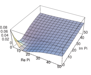
which is corresponds to the Fubini-Study metric (2.11) plays an important role in gauge transformations of the functional frame. Namely, we will show that the connection (2.15) determines the natural intrinsic gauge potential of a local frame rotation in a tangent space of CP(N) and, therefore, modification of field dynamical variables. Relationships between the Goldsone and Higgs modes arise in an absolutely natural way (see Fig.1).

Figure 1: The connection (2.15) in the case CP(1). The value of $1/R+\Gamma^{i}_{kl}$ is shown. Radial directions are related to the Goldstone modes of “deformations” of quantum state. Angular rotations represent the Higgs modes of the gauge transformations in every point of a geodesic. All geodesics are subjected to a “rigid rotation” under the action of the isotropy group.

Below we shall discuss a simple model of a “wrapping” of this underlying structure into the gauge (compensation) field in the reference Minkowski spacetime.

3 Generalized nonlinear Klein-Gordon equation

The key idea is associated with a model for a single quantum particle as an extended field dynamical system. We will to interpret internal local coordinates (2.5) as relative Fourier componets of some wave packet in reference Minkowski spacetime. Therefore the “Hamilton pre-system” in CP(N) is “wrapped” in the shell of a gauge field in ordinary spacetime and one has, hence, a non-local extended dynamical field configuration. It should play the role of a model of non-local quantum particles in the framework of the causal approach to quantum theory [4, 5]. For the global ‘shaping” of this configuration, the Klein-Gordon field configuration with “Poincaré-radial” Lagrangian for non-linear interaction has been chosen. This Lagrangian depends only on the “radial” variable $\rho$ , i.e. $\Phi=\Phi(\rho)$, where $\rho^{2}=x_{\mu}x^{\mu}$ and $x^{\mu}$ Since $\Phi_{,\mu}=\frac{\partial\Phi}{\partial x^{\mu}}=\frac{x_{\mu}}{\rho}\frac{d\Phi}{d\rho}$ and $\Phi^{,\mu}=\frac{\partial\Phi}{\partial x_{\mu}}=\frac{x^{\mu}}{\rho}\frac{d\Phi}{d\rho}$, a Lagrangian density may be written as

$$\cal L\rm=\frac{1}{2}\Phi^{*}_{\mu}\Phi^{\mu}-U(\Phi(\rho))=\frac{1}{2}\left|\frac{d\Phi}{d\rho}\right|^{2}-U(\Phi(\rho)),$$ (3.1)

where we have assumed a general form for the effective self-interaction term $U(\Phi(\rho))$. The equation of motion of the scalar field acquires the form of the ordinary differential (nonlinear in general) equation

$$\frac{d^{2}\Phi^{*}}{d\rho^{2}}+(3/\rho)\frac{d\Phi^{*}}{d\rho}+2\frac{\partial U(\Phi(\rho))}{\partial\Phi}=0.$$ (3.2)

This equation has been used in the problem of vacuum decay (see ([12]) and references therein). If the potential $U(\Phi(\rho))$ has the form $U(\Phi(\rho))=\frac{1}{2}(mc/\hbar)^{2}\Phi^{*}\Phi=\frac{1}{2}\alpha^{2}|\Phi|^{2}$, then (3.2) is the linear Lommel equation

$$\frac{d^{2}\Phi^{*}}{d\rho^{2}}+(3/\rho)\frac{d\Phi^{*}}{d\rho}+\alpha^{2}\Phi^{*}=0,$$ (3.3)

for which a solution is expressed in the Bessel function $\Phi=\rho^{-1}J_{-1}(\alpha\rho)$. However a “deformation” of these solutions into solutions of some effectively nonlinear Klein-Gordon equation by the geodesic flow is interesting for our purpose. If we choose the the classical radius of the electron $r_{0}=\frac{e^{2}}{mc^{2}}$ as the unit of distance scale $\rho=xr_{0}$, then $(mc/\hbar)^{2}$ in (3.3) becomes the fine structure constant $\alpha=\frac{e^{2}}{\hbar c}$. Let’s suppose $y=(\rho/r_{0})^{2}$. One can represent a solution of (3.3) in the $y$-variable as a Fourier series

$$|\Phi>=x^{-1}J_{-1}(\alpha x)=\sum_{k=0}^{\infty}\Phi^{k}|k,y>,$$ (3.4)

where

$$\Phi^{m}=\frac{-1}{2^{m}m!\sqrt{\pi}}\int_{-\infty}^{\infty}dy\exp(-\frac{y^{2}}{2})H_{m}(y)y^{-1/2}J_{1}(\alpha y^{1/2})$$ (3.5)

and $|n,y>=(2^{n}n!\sqrt{\pi})^{-1/2}\exp(-y^{2}/2)H_{n}(y)$ is complete set of orthogonal Hermitian functions on the interval $(-\infty,\infty)$. Our geodesic flow acts on these Fourier components. It is convenient to transform the state covector (3.5) to the “vacuum” form (2.1) by the set of matrices $\hat{G}$ as followes [7]. In order to find the elements $f^{i}$ of the generator of the geodesic flow for deformation of the vacuum state toward the solution (3.4) one should note that if result of the periodic geodesic “deformation” of the initial solution of

$$|\Psi(\tau,g,y)>=\sum^{\infty}_{m,n=0}|n,y>\Phi^{m}[\hat{G}\hat{T}(\tau,g)\hat{G}^{-1}]^{n}_{m}$$ (3.6)

is not so far from (2.1), then one can span them by an unique geodesic $(1,0,...,0)\hat{T}(\tau,g)=R^{-1}(\Phi^{0},\Phi^{1},...,\Phi^{N})$. It may be shown that $cos\Theta=|\Phi^{0}|/R$, $|f^{i}|=g|\Phi^{i}|(R^{2}-|\Phi^{0}|^{2})^{-1/2}$ and $\arg f^{i}=\arg\Phi^{i}$ (up to the general phase). Thus “rate” and direction of the transformation of the vacuum vector into the solution of the Lommel equation is determined by the matrix $\hat{P}=\hat{G}^{-1}(\Phi)\hat{B}(\Phi)\hat{G}(\Phi)$.

In order to establish relationships between “internal” parameters in $CP(\infty)$ and a propagation of the scalar field near the light cone in the “reference spacetime”, we should “lift” a geodesic deformation of the initial Fourier components into the fiber bundle. Namely, if we assume that in accordance with the “superequivalence principle” an infinitesimal geodesic “shift” of field dynamical variables could be compensated by an infinitesimal transformations of the basis in Hilbert space, then one can get some effective self-interaction potential as an addition to the mass term in original Klein-Gordon equation in the Lommel’s form (3.3). We will label hereafter vectors of the Hilbert space by Dirac’s notations $|...>$ and tangent vectors to CP(N) or $CP(\infty)$ (field dynamical variables) by arrows over letters, $\vec{\xi}\in T_{\Pi}CP(\infty)$, for example. Then one has a definition of the rate of a state vector changing $|v(x)>=-(i/\hbar)\hat{P}|\Psi(x)>$. The “descent” of the vector field $|v(x)>$ onto the base manifold $CP(\infty)$ is a mapping by the two formulas: $f:\cal H\rm\to CP(\infty)$, i.e. like (2.5) $f:(\Psi^{0},...,\Psi^{a},...)=(R\frac{\Psi^{1}}{\Psi^{0}},...,R\frac{\Psi^{i}}{\Psi^{0}},...)=(\Pi^{1},...,\Pi^{i},...)$ and

$$\vec{\xi}=f_{*(\Psi^{0},...,\Psi^{m},...)}|v(x)>=\frac{d}{d\tau}(R\frac{\Psi^{1}}{\Psi^{0}},...,R\frac{\Psi^{i}}{\Psi^{0}},...)\Bigl{|}_{0}$$ (3.7)

$$=-(i/\hbar)[P^{1}_{0}+(P^{1}_{k}-P^{0}_{k}\Pi^{1})\Pi^{k},...,P^{i}_{0}+(P^{i}_{k}-P^{0}_{k}\Pi^{i})\Pi^{k},...].$$ (3.8)

This operator determines a field dynamicl variable $\vec{\xi}$ (3.8). At a point $\Pi+\delta\Pi$ in $CP(\infty)$ the “shifted” field $\vec{\xi}+\delta\vec{\xi}$ $=\vec{\xi}+\frac{\delta\vec{\xi}}{\delta l}\delta l$ contains the derivative $\frac{\delta\vec{\xi}}{\delta l}$, which is not, in the general case, a tangent vector to $CP(\infty)$, but the covariant derivative $\frac{\Delta\xi^{i}}{\delta l}$ $=\frac{\delta\xi^{i}}{\delta l}+\Gamma^{i}_{km}\xi^{k}\frac{\delta\Pi^{m}}{\delta l}$ is a tangent vector to $CP(\infty)$. Now we should “lift” the new tangent vector $\xi^{i}+\Delta\xi^{i}$ into the original Hilbert space $\cal H\rm$, that is, one needs to realize two inverse mappings: $f^{-1}:CP(\infty)\to\cal H\rm$

$$f^{-1}(\Pi^{1}+\Delta\Pi^{1},...,\Pi^{i}+\Delta\Pi^{i},...)=[\Psi^{0},\Psi^{1}+\Psi^{0}\Delta\Pi^{1},...,\Psi^{i}+\Psi^{0}\Delta\Pi^{i},...]$$ (3.9)

and then

$$f^{-1}_{*\Pi+\delta\Pi}(\vec{\xi}+\Delta\vec{\xi})=[v^{0},v^{1}+\frac{d}{d\tau}(\Psi^{0}\Delta\Pi^{1})\Big{|}_{0},...,v^{i}+\frac{d}{d\tau}(\Psi^{0}\Delta\Pi^{i})\Big{|}_{0},...].$$ (3.10)

It may be shown in our original Hilbert space $\cal H\rm$ that the term $|dv>$ arises as an additional rate of a change of some general state vector $|\Psi>$

$$|dv>=-\frac{i}{\hbar}d\hat{P}|\Psi>=[0,\frac{d}{d\tau}(\Psi^{0}\Delta\Pi^{1})\Bigl{|}_{0}|1,x>,...,\frac{d}{d\tau}(\Psi^{0}\Delta\Pi^{i})\Bigl{|}_{0}|i,x>,...],$$ (3.11)

where $\Delta\Pi^{i}=-\Gamma^{i}_{km}\xi^{k}d\Pi^{m}\tau$. Then $\Delta U=\frac{\delta U}{\delta\Pi^{i}}d\Pi^{i}+\frac{\delta U}{\delta\Pi^{*i}}d\Pi^{*i}$ where $\frac{\delta U}{\delta\Pi^{m}}=-\hbar\Gamma^{i}_{km}\xi^{k}|i,y>$ may be treated as an “instantaneous” self-interacting potential of the scalar configuration associated with the infinitesimal gauge transformation of the local frame with coefficients (2.15). That is the state vector (3.9) inherits the geomeric structure of the $CP(\infty)$ and perturbed Lagrangian is as follows:

$$\cal L^{\prime}\rm=\cal L\rm(\Psi+\Delta\Psi)=(\Psi+\Delta\Psi)^{m*}\frac{\partial<m,y|}{\partial t}\frac{\partial|n,y>}{\partial t}(\Psi+\Delta\Psi)^{n}$$ (3.12)

$$-(\Psi+\Delta\Psi)^{m*}\nabla<m,y|\nabla|n,y>(\Psi+\Delta\Psi)^{n}$$ (3.13)

$$-\alpha^{2}(\Psi+\Delta\Psi)^{m*}<m,y|n,y>(\Psi+\Delta\Psi)^{n},$$ (3.14)

where $\Delta\Psi^{i}=-\Psi^{0}\Gamma^{i}_{km}\xi^{k}d\Pi^{m}\tau$ [4]. Note, spacetime derivatives of the basis Hermitian functions $\nabla|n,y>$, $\frac{\partial|n,y>}{\partial t}$ only arise in the formula for Lagrangian density. On the other hand, only Fourier components (3.5) are subjected to the variation by the geodesic flow. Equation of motion of the self-interacting field configuration-droplet may be obtained from variation of the Lagrangian relative to the variation of $|\Psi>$. One then has a generalized Klein-Gordon equation

$$\Box\Psi^{*}+\Box A^{*}+\Psi^{*}_{\mu\mu}\frac{\delta A_{\mu}}{\delta\Psi_{\mu}}+\Psi^{*}_{\mu}\frac{\delta A_{\mu\mu}}{\delta\Psi_{\mu}}+\alpha^{2}(\Psi^{*}+\Delta\Psi^{*}+\Psi^{*}\frac{\delta\Delta\Psi}{\delta\Psi})=0,c.c.,$$ (3.15)

where $A_{\mu}=\frac{\partial\Delta\Psi}{\partial x^{\mu}}$,$A_{\mu\mu}=\frac{\partial\Delta\Psi}{\partial x^{\mu}\partial x^{\mu}}$, $\Psi_{\mu}=\frac{\partial\Psi}{\partial x^{\mu}}$,$\Psi_{\mu\mu}=\frac{\partial\Psi}{\partial x^{\mu}\partial x^{\mu}}$, and for enough small $\tau$

$$\Delta\Psi^{i}=-g\Psi^{0}\tau^{2}(1+\frac{|\Psi^{0}|^{2}}{R^{2}})^{-1/2}\Gamma^{i}_{km}\xi^{k}\Psi^{m}.$$ (3.16)

If the radius $R$ of the sectional curvature $1/R^{2}$ of the projective Hilbert space goes to infinity, one obtains the ordinary Klein-Gordon equation. We can hope that non-trivial metric and topology of the projective Hilbert space endows global solutions of non-linear wave equation with interesting physical properties. In the general case the curvature of the projective state space influences the wave dispersion of a nonliner solution of the equation. It may be treated as a base of the experimental testing of a quantum nonlinearity. This topic will be investigated in the near futures.

ACKNOWLEDGEMENTS

I thank Yuval Ne’eman and Larry Horwitz for numerous useful discussions and Yakir Aharonov for attention to this work. This research was supported in part by grant PHY-9307708 of the National Science Foundation, and by grant of the Ministry of Absorption of Israel.

References

- [1] S. Weinberg, Ann. Phys. (N.Y.), 194, 336 (1989).
- [2] N.Gisin, Phys.Lett. A, 143 1 (1990).
- [3] H.-D.Doebner and G.A.Goldin, Phys.Rev.A 54, No.5 3764 (1996).
-
[4]
P.Leifer, Superrelativity as a unification of quantum
theory and relativity,
Preprint quant-ph/9610030. -
[5]
theory and relativity (II),
Preprint gr-qc/9612002. -
[6]
P.Leifer, Quantum theory Requires Gravity and Superrelativity,
Preprint gr-qc/9610043. -
[7]
P.Leifer, Why we can not see the curvature of the quantum
state space?
Preprint gr-qc/9701006. -
[8]
P.Leifer, Superrelativity as an Element of a Final Theory,
(to be published in Found.Phys.,February 1997). - [9] A.Einstein, Die Grundlage der allgemeinen Relativitätstheorie, Ann.Phys., 49 769 (1916).
- [10] Wei-Min Zhang, Da Hsuan Feng, Phys.Rep.252, 1 (1995).
[11]
S. Kobayashi and K. Nomizu,Foundations of Differntial Geometry,vol.II,
(Interscience Publishers, New York-London-Sydney, 1969). -
[12]
S.Weinberg,The Quantum Theory of Fields, vol.II,
(Cambridge University Press, 1996).