Critical Couplings in the Nambu–Jona-Lasinio Model
with the Constant Electromagnetic Fields

Abstract

A detailed analysis is performed for the Nambu–Jona-Lasinio model coupled with constant (external) magnetic and/or electric fields in two, three, and four dimensions. The infrared cut-off is essential for a well-defined functional determinant by means of the proper time method. Contrary to the previous observation, the critical coupling remains nonzero even in three dimensions. It is also found that the asymptotic expansion has an excellent matching with the exact value.

The four-fermi interaction model by Nambu and Jona-Lasinio (NJL) [1] has been discussed to investigate the dynamical symmetry breaking (DSB) in a number of cases in two, three, and four dimensions. Especially interesting situations are found such that NJL is coupled to external sources, which enables us to peep into detailed structures of DSB, giving informations of the chiral symmetry breaking in the QCD vacuum, the planar ($2+1$-dimensional) dynamics in solid state physics, or the early universe when coupled to a curved space-time [2]. The NJL model minimally coupled to the electromagnetic fields is discussed yielding the result that the electric field destabilizes DSB but the magnetic field stabilizes it [3]. In the pure magnetic field case, Gusynin, Miransky, and Shovkovy made detailed discussions to find that there occurs the mass generation even at the weakest attractive interaction [4] (in $2+1$ dimensions) and emphasize it by means of the dimensional reduction [5]. This implies that the critical coupling is zero even if the applying magnetic field is infinitesimal (in the $2+1$-dimensional case) which might however contradict a naïve expectation. The motivation for this work lies here.

We start with the partition function of the NJL model minimally coupled to the external electromagnetic field in $D$ (space-time) dimensions:

$$Z[A]\!\! \equiv \!\!\int{\mathcal{D}}\psi{\mathcal{D}}\overline{\psi}\exp\left[-\int d^{D}x\Bigl{[}\overline{\psi}\Bigl{\{}\gamma_{\mu}\bigl{(}\partial_{\mu}-iA_{\mu}\bigr{)}\Bigr{\}}\psi-{g^{2}\over 2}\left\{\bigl{(}\overline{\psi}\psi\bigr{)}^{2}+\bigl{(}\overline{\psi}i\gamma_{5}\psi\bigr{)}^{2}\right\}\Bigr{]}\right]$$

$$= \!\!\int{\mathcal{D}}\sigma{\mathcal{D}}\pi{\mathcal{D}}\psi{\mathcal{D}}\overline{\psi}\exp\left[-\int d^{D}x\Bigl{[}{1\over 2g^{2}}\bigl{(}\sigma^{2}+\pi^{2}\bigr{)}+\overline{\psi}\Bigl{\{}\gamma_{\mu}\bigl{(}\partial_{\mu}-iA_{\mu}\bigr{)}+\bigl{(}\sigma+i\pi\gamma_{5}\bigr{)}\Bigr{\}}\psi\Bigr{]}\right]\ ,$$

where the electromagnetic coupling constant has been absorbed in the definition of $A_{\mu}$ and the auxiliary fields, $\sigma$ and $\pi$, have been introduced as usual. The Euclidean metric has been employed. The fermionic integration gives the functional determinant: (this can be considered as the definition of the fermionic functional measure if some calculative way would be provided as in the follows:)

$$\int{\mathcal{D}}\psi{\mathcal{D}}\overline{\psi}\exp\left[\overline{\psi}\Bigl{\{}\gamma_{\mu}\bigl{(}\partial_{\mu}-iA_{\mu}\bigr{)}+\bigl{(}\sigma+i\pi\gamma_{5}\bigr{)}\Bigr{\}}\psi\right]\equiv\det\Bigl{[}\gamma_{\mu}\bigl{(}\partial_{\mu}-iA_{\mu}\bigr{)}+\bigl{(}\sigma+i\pi\gamma_{5}\bigr{)}\Bigr{]}\ .$$ (2)

We then perform the semiclassical approximation, that is, shift $\sigma\rightarrow m+\sigma^{\prime};\ \pi\rightarrow\pi^{\prime}$ and assign $\sigma^{\prime}$ and $\pi^{\prime}$ as the new integration variables to find

$$Z[A]=\exp\left[-VT{m^{2}\over 2g^{2}}+{\rm Tr}\ln\Bigl{[}\gamma_{\mu}\bigl{(}\partial_{\mu}-iA_{\mu}\bigr{)}+m\Bigr{]}\right]\Bigl{(}1+O(\mbox{$2$-loop})\Bigr{)}\equiv{\mathrm{e}}^{-VT{\mbox{\Large$v$}}_{\rm T}}\Bigl{(}1+O(\mbox{$2$-loop})\Bigr{)}\ ,$$ (3)

where $V$ is the $(D-1)$-dimensional volume of the system and $T$ is the Euclidean time interval and the trace operation, designated by Tr, must be taken with respect to the space-time as well as the gamma matrices, meanwhile tr implies the trace for the gamma matrices. We call ${\mbox{\Large$v$}}_{\rm T}$ the total potential. Finally it should be understood that the terms of $O(\mbox{two-loop})$ are composed by the $\pi^{\prime},\sigma^{\prime}$ integrations.

The functional determinant, $I(D)\equiv{\rm Tr}\ln\Bigl{[}\gamma_{\mu}\bigl{(}\partial_{\mu}-iA_{\mu}\bigr{)}+m\Bigr{]}$ can be defined, as is mentioned above, with the aid of the proper time method, and is exactly calculable when the field strength is constant [6]:

$$I(D)=-{VT\over 2}\lim_{s\rightarrow 0}{1\over(4\pi)^{D/2}}\int_{0}^{\infty}d\tau\ \tau^{s-D/2-1}e^{-\tau m^{2}}\left[\det\Bigl{(}{\sin\tau F\over\tau F}\Bigr{)}\right]^{-1/2}{\rm tr}\ \exp\left({\tau\over 2}\sigma_{\mu\nu}F_{\mu\nu}\right)\ ,$$ (4)

where $F$ stands for $D\times D$ matrix $(F_{\mu\nu})$ and $\sigma_{\mu\nu}=\bigl{[}\gamma_{\mu},\gamma_{\nu}\bigr{]}/2i$. It should be noted that (4) holds even for odd dimensions, $D=3$: there is no chiral transformation but by introducing an additional fermion we have a four-component theory to be able to discuss the chiral symmetry in a parallel manner as in $D=4$ or $2$ [7]. Calculating the determinant and the trace, we obtain

$$I(D)=-VT{{\rm C}^{(D)}F_{D}\over\pi^{D/2}}\lim_{s\rightarrow 0}\int_{0}^{\infty}d\tau\ \tau^{s-D/2}e^{-\tau m^{2}}\coth\tau F_{D}$$ (5)

with

$$F_{D}\equiv\left\{\begin{array}[]{cc}{\displaystyle E\ ,}&{\displaystyle D=2\ ,}\\ \vspace{1ex}\cr{\displaystyle\sqrt{B^{2}+{\mathbit E}^{2}}\ ,}&{\displaystyle D=3\ ,}\\ \vspace{1ex}\cr{\displaystyle\sqrt{{\mathbit B}^{2}+{\mathbit E}^{2}}\ ,}&{\displaystyle D=4\ ,}\end{array}\right.\hskip 20.0pt{\rm C}^{(D)}\equiv\left\{\begin{array}[]{cc}{\displaystyle{1\over 4}\ ,}&{\displaystyle\ D=2,\ 3\ ,}\\ \vspace{1ex}\cr{\displaystyle{1\over 8}\ ,}&{\displaystyle D=4\ .}\end{array}\right.$$ (6)

However it should be noted that in the four-dimensional case we have assumed that ${\mathbit B}\cdot{\mathbit E}=0$ otherwise we have

$$I_{\rm exact}(D=4)=-VT\lim_{s\rightarrow 0}{F_{+}F_{-}\over 8\pi^{2}}\int_{0}^{\infty}d\tau\ \tau^{s-1}e^{-\tau m^{2}}\coth\tau F_{+}\coth\tau F_{-}\ ,$$ (7)

where $F_{\pm}\equiv\left\{\bigl{|}{\mathbit B}+{\mathbit E}\bigr{|}\pm\bigl{|}{\mathbit B}-{\mathbit E}\bigr{|}\right\}/2$. (A detailed calculation will be published elsewhere [8].)

In this paper we will confine ourselves in the case ${\mathbit B}\cdot{\mathbit E}=0$, therefore, in (5) for brevity. Although the integral has entirely been regularized if an analytic continuation is made for $s$, it is better to introduce an ultraviolet cut-off $\Lambda$ with dimension in order to grasp a physical situation as is done in the ordinary gap equation [1]. Moreover an infrared cut-off must be necessary in this case because we know that there arises an infrared divergence when external fields are coupled to the massless state. A more careful treatment is therefore required for the discussion on the transition from the massless to the massive state under external fields. We then consider instead of (5)

$$I_{\rm r}(D)\equiv-VT{{\rm C}^{(D)}F_{D}\over\pi^{D/2}}\int_{1\over\Lambda^{2}}^{\infty}d\tau\ \tau^{-D/2}e^{-\tau(m^{2}+\epsilon)}\coth\tau F_{D}\ ,$$ (8)

where $\Lambda$ is the ultraviolet cut-off and $\epsilon$ is the infrared one to ensure the existence of the massless limit: $m^{2}\longrightarrow 0$. It should be noted that they are gauge and Lorentz invariant. With these regularizations the integral (8) now becomes well-defined at any time. Now the total potential in (3) reads

$${\mbox{\Large$v$}}_{\rm T}={m^{2}\over 2g^{2}}+{{\rm C}^{(D)}F_{D}\over\pi^{D/2}}\int_{1\over\Lambda^{2}}^{\infty}d\tau\ \tau^{-D/2}e^{-\tau(m^{2}+\epsilon)}\coth\tau F_{D}\ ,$$ (9)

whose explicit value can be estimated such that

$${\mbox{\Large$v$}}_{\rm T} = {m^{2}\over 2g^{2}}+{m^{2}+\epsilon\over 4\pi}\left[\gamma+\ln{m^{2}+\epsilon\over\Lambda^{2}}-\ln a+{1\over 2a}\bigl{(}\ln{a\over 2\pi}+2\ln\Gamma(a)\bigr{)}\right]\ ;\hskip 45.20819ptD=2\ ,$$ (10)

$${\mbox{\Large$v$}}_{\rm T} = {m^{2}\over 2g^{2}}-{\left(m^{2}+\epsilon\right)\Lambda\over 2\pi^{3/2}}-{\left(m^{2}+\epsilon\right)^{3/2}\over 2\pi^{3/2}}\left[{\sqrt{\pi}\over 2a}-{\sqrt{\pi}\over a^{3/2}}\zeta\!\left(-{1\over 2},a\right)\right]\ ;\hskip 62.43036ptD=3\ ,$$ (11)

$${\mbox{\Large$v$}}_{\rm T} = {m^{2}\over 2g^{2}}-{\bigl{(}m^{2}+\epsilon\bigr{)}\Lambda^{2}\over 8\pi^{2}}+{\bigl{(}m^{2}+\epsilon\bigr{)}^{2}\over 16\pi^{2}}\left[\left(1+{1\over 6a^{2}}\right)\left(1-\gamma-\ln{m^{2}+\epsilon\over\Lambda^{2}}+\ln a\right)\right.$$

$$\hskip 206.66602pt\left.-{1\over a}\ln a-{2\over a^{2}}\zeta^{\prime}\!\!\left(-1,a\right)\right]\ ;\ \ D=4\ ,$$

where $a\equiv(m^{2}+\epsilon)/2F_{D}$, $\Gamma(a)$, $\gamma$ is the gamma function, Euler’s constant respectively, $\zeta(s,a)$ is Riemann’s zeta function, and $\zeta^{\prime}(s,a)\equiv d\zeta(s,a)/ds$. We have discarded terms of $O\bigl{(}m^{2}/\Lambda^{2}\bigr{)},O\bigl{(}F_{D}/\Lambda^{2}\bigr{)},$ and also purely $\Lambda$-dependent terms to arrive at the expressions; (10) $\sim$ (LABEL:potfour).

Since our interest is to know the change of the system undergone by switching on the external field, the parameter, $a$, can be considered very large, $a\sim\infty$. Therefore the asymptotic expansion for $\ln\Gamma(a),\ \zeta(s,a)$ can be utilized to give

$${\mbox{\Large$v$}}_{\rm T} \stackrel{{\scriptstyle a\rightarrow\infty}}{{\longrightarrow}} {m^{2}\over 2g^{2}}+{m^{2}+\epsilon\over 4\pi}\left(\gamma+\ln{m^{2}+\epsilon\over\Lambda^{2}}-1\right)+{F_{2}^{2}\over 12\pi\left(m^{2}+\epsilon\right)}\ ;\hskip 124.86072ptD=2\ ,$$ (13)

$${\mbox{\Large$v$}}_{\rm T} \stackrel{{\scriptstyle a\rightarrow\infty}}{{\longrightarrow}} {m^{2}\over 2g^{2}}-{\left(m^{2}+\epsilon\right)\Lambda\over 2\pi^{3/2}}+{\left(m^{2}+\epsilon\right)^{3/2}\over 3\pi}+{F_{3}^{2}\over 12\pi\left(m^{2}+\epsilon\right)^{1/2}}\ ;\hskip 122.70795ptD=3\ ,$$ (14)

$${\mbox{\Large$v$}}_{\rm T} \stackrel{{\scriptstyle a\rightarrow\infty}}{{\longrightarrow}} {m^{2}\over 2g^{2}}-{\left(m^{2}+\epsilon\right)\Lambda^{2}\over 8\pi^{2}}+{\left(m^{2}+\epsilon\right)^{2}\over 16\pi^{2}}\left({3\over 2}-\gamma-\ln{m^{2}+\epsilon\over\Lambda^{2}}\right)-{F_{4}^{2}\over 24\pi^{2}}\left(\gamma+\ln{m^{2}+\epsilon\over\Lambda^{2}}\right)\ ;D=4\ .$$ (15)

It should be stressed that owing to the infrared cut-off, $\epsilon$, we can rely on the asymptotic expansion even in the case $m=0$: here we regard the infinitesimal size of external fields as, $F_{D}<<\epsilon$.

The gap equation is therefore obtained for $m^{*}\neq 0$ as

$$\hskip 43.05542pt-{2\pi\over g^{2}} = \gamma+\ln x-{{\mathcal{F}}_{2}^{2}\over 3x^{2}}\ ;\hskip 129.16626ptD=2\ ,$$ (16)

$$\hskip 43.05542pt1-{\pi^{3/2}\over g^{2}\Lambda} = \pi^{1/2}\left[x^{1/2}-{{\mathcal{F}}_{3}^{2}\over 12x^{3/2}}\right]\ ;\hskip 99.02747ptD=3\ ,$$ (17)

$$\hskip 43.05542pt1-{4\pi^{2}\over g^{2}\Lambda^{2}} = x\left(1-\gamma-\ln x\right)+{{\mathcal{F}}_{4}^{2}\over 3x}\ ;\hskip 99.02747ptD=4\ ,$$ (18)

where we have introduced the dimensionless quantities; $x\equiv({m^{*}}^{2}+\epsilon)/\Lambda^{2}$, ${\mathcal{F}}_{D}\equiv F_{D}/\Lambda^{2}$. (Recall that the mass-dimension of the gauge field is always one because of the inclusion of the coupling constant.) Moreover the stability condition, $\partial^{2}{\mbox{\Large$v$}}_{\rm T}/\partial m^{2}\Bigr{|}_{m^{*}}\geq 0$, must be fulfilled; which reads $df(x)/dx\equiv f^{\prime}(x)\geq 0$. Since if we write the right-hand-side of the relations (16) $\sim$ (18) generically as $f(x)$ we find $\partial^{2}{\mbox{\Large$v$}}_{\rm T}/\partial m^{2}\Bigr{|}_{m^{*}}\sim xf^{\prime}(x)$. In addition, the global minimum condition, ${\mbox{\Large$v$}}_{\rm T}\bigr{|}_{m=0}>{\mbox{\Large$v$}}_{\rm T}\bigr{|}_{m^{*}}$, must be satisfied in order to assign $m^{*}$ as the true minimum; since it may happen that $\bigl{.}{\mbox{\Large$v$}}_{\rm T}\bigr{|}_{m=0}\leq\bigl{.}{\mbox{\Large$v$}}_{\rm T}\bigr{|}_{m^{*}}$ under the influence of the external field.

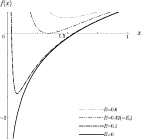
(a) (b)
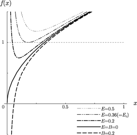
(c)

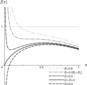
Figure 1: (a), (b), and (c): the plot of the right hand sides of (16), (17), and (18). ${\mathcal{F}}_{D}$ is read as ${\mathcal{F}}_{D}=-iE$ and ${\mathcal{F}}_{D}=B$ . Solutions of the gap equations are found from the intersection of $f(x)$ and the horizontal line depicting the coupling dependence. From (16) $\sim$ (18) and the stability condition, such intersections should be in the region: (i) under thin-dashed horizontal line (at $0$ in two dimensions and $1$ in three and four dimensions), (ii) of $f(x)$ with non-negative gradient. The critical electric fields are defined by those over which no chiral symmetry breaking occurs in any coupling, and characterized by upper curves attaching to the thin-dashed horizontal line in two and three dimensions or by the minimum curve of monotonically decreasing in four dimensions. Due to the infrared cut-off, $m^{*2}=0$ does not correspond to $x=0$ but $x=\epsilon/\Lambda^{2}$. Note that the critical coupling $g_{c}$ remains finite against $B\neq 0$ as long as $\epsilon/\Lambda^{2}$ is finite.

Let us consider specific cases: a purely magnetic as well as electric field case. We first start with the magnetic field case, that is in three and four dimensions: $F\mapsto|{\mathbit B}|$ in (17) and (18). From Figure.1(b),(c) it can be recognized that the magnetic field reduces the critical coupling $g_{c}$. It should be noted that even in three dimensions $g_{c}$ never reaches zero. If we take $\epsilon\rightarrow 0$, while keeping $|{\mathbit B}|\neq 0$, (implying $x\rightarrow 0$ in the figures), $g_{c}$ would tend to zero, which, however, cannot be allowed as far as the external fields are present. In this way the observation by Gusynin et al. [5] is not true. They have simply ignored the infrared divergences to get the $g_{c}=0$ result and interpreted it by means of the dimensional reduction.

Next we take the purely electric field case in two, three, and four dimensions: $F\rightarrow-i|{\mathbit E}|$. (Recall that we have been in the Euclidean world.) Again from Figure.1(a)$\sim$(c), it is apparent that stronger the electric field becomes larger the critical coupling $g_{c}$. Electric fields thus restore the symmetry when they overreach the point $|{\mathbit E}_{c}|$ (whose value is seen in the figures). The observation is consistent with Klevansky et al. [3] (but they have also ignored the infrared divergences.)

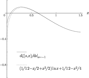
Figure 2: The asymptotic expansion and the exact curve in four dimensions: the dashed (solid) curve is the asymptotic expansion ($\zeta^{\prime}(-1,x)$). Note that the matching is excellent over the whole region except the origin.

So far we have utilized the asymptotic expansion to the potential (10) to (LABEL:potfour): $a\equiv(m^{2}+\epsilon)/2F_{D}\sim\infty$. Then it seems that the discussions above are plausible only in the region where the strength of the external fields is tiny compared to the (generated) mass. However as can be seen from Figure.2 (of four dimensions), the asymptotic expansion, (15), matches with the exact value up to $a\sim 0.5$ and, moreover, does not deviate from it except around the origin. (The situation is the same for two and three dimensions.) Therefore the exact form of the potential in four dimensions depicted as Figure.3 remains almost unchanged after employing the asymptotic expansion and we can recognize that our minimum is indeed the global minimum.

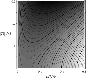
(a)                 (b)

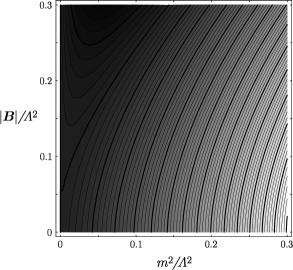
Figure 3: The contour plots of the total potential with magnetic field (a) at $4\pi^{2}/g^{2}\Lambda^{2}=0.85$ and (b) at $4\pi^{2}/g^{2}\Lambda^{2}=1.15$ in four dimensions. The potential has been adjusted to vanish at $m^{2}/\Lambda^{2}=0$ and drawn in the unit of $\Lambda^{4}/8\pi^{2}$. Note that the adjustment is possible due to the infrared cut-off $\epsilon$ whose value is $\epsilon/\Lambda^{2}=0.00001$. The thick contours imply the height difference of $0.01$. The minimum of the potential moves to the right as the magnetic field becomes stronger.

Accordingly we can increase external fields larger than the mass even under the asymptotic expansion. It should, however, bear in mind that an arbitrarily large electric field cannot be allowed; since there emerges an imaginary part in the potential [3] when $a\rightarrow 0$. Intuitively speaking when the electric field exceeds the threshold of the particle, $|{\mathbit E}|>m^{2}$, a pair creation occurs, which leads to instability of the vacuum. (The phenomena is closely related to the Klein paradox and is well-known [9].)

In four dimensions, we have assumed ${\mathbit B}\cdot{\mathbit E}=0$ so that we need not worry about the chiral anomaly which, however, must be taken into account in the non-abelian case. Therefore the full calculation to (7) is desirable and will be seen in our next work [8].

Acknowledgment

The authors thank to Kenzo Inoue and Koji Harada for valuable discussions.

References

• [1] Y. Nambu and G. Jona-Lasinio, Phys. Rev. 122 (1961) 345.
• [2] T. Inagaki, T. Muta and S. D. Odintsov, Mod. Phys. Lett. A 8 (1993) 2117.
• [3] S. P. Klevansky and R. H. Lemmer, Phys. Rev. D 39 (1989) 3478.
• [4] V. P. Gusynin, V. A. Miransky, I. A. Shovkovy, Phys. Rev. D 52 (1995) 4718.
• [5] V. P. Gusynin, V. A. Miransky, I. A. Shovkovy, Phys. Lett. B 349 (1995) 477.
• [6] See for example, C. Itzykson and J. B. Zuber, “Quantum Field Theory” (McGraw-Hill, New York, 1980) page 100.
• [7] T. W. Appelquist, M. Bowick, D. Karabali, and L. C. R. Wijewardhana, Phys. Rev. D 33 (1986) 3704.
• [8] M. Ishi-i, T. Kashiwa, and N. Tanimura; being prepared for the publication.
• [9] See for example, W. Greiner, B. Müller, and J. Rafelski, “Quantum Electrodynamics of Strong Fields” (Springer-Verlag, Berlin, 1985) chap. 5 and 6.