Casimir effect in dielectrics: Bulk Energy Contribution

In a recent series of papers, Schwinger discussed a process that he called the Dynamical Casimir Effect. The key essence of this effect is the change in zero-point energy associated with any change in a dielectric medium. (In particular, if the change in the dielectric medium is taken to be the growth or collapse of a bubble, this effect may have relevance to sonoluminescence.) The kernel of Schwinger’s result is that the change in Casimir energy is proportional to the change in volume of the dielectric, plus finite-volume corrections. Other papers have called into question this result, claiming that the volume term should actually be discarded, and that the dominant term remaining is proportional to the surface area of the dielectric. In this communication, which is an expansion of an earlier letter on the same topic, we present a careful and critical review of the relevant analyses. We find that the Casimir energy, defined as the change in zero-point energy due to a change in the medium, has at leading order a bulk volume dependence. This is in full agreement with Schwinger’s result, once the correct physical question is asked. We have nothing new to say about sonoluminescence itself.

I Schwinger’s calculation

Several years ago, the late Julian Schwinger wrote a series of papers [1, 2, 3] wherein he calculated the Casimir energy released in the collapse of a spherically symmetric bubble or cavity. (For the evolution of Schwinger’s ideas on this topic, see [4, 5, 6, 7].) Using source theory, he derived in a simple and elegant way a formula for the energy release involved in the collapse. He found from a straightforward application of the action principle that (for each polarization state) the “dielectric energy, relative to the zero energy of the vacuum, [is given] by

$$E=-V\int\frac{d^{3}\vec{k}}{(2\pi)^{3}}\frac{1}{2}[\hbar c]k\left(1-\frac{1}{\sqrt{\epsilon}}\right).$$ (1)

So the Casimir energy of a uniform dielectric is negative”. This was then applied by Schwinger as a model for sonoluminescence.

From this, and following Schwinger, we conclude that a dielectric slab of material with a spherical vacuum cavity of radius $R$ has a higher Casimir energy than the slab of material with the vacuum cavity re–filled with material of the same dielectric constant. This energy (per polarization state) can be computed by introducing an ultraviolet momentum cut-off $K$ into the previous expression for the energy 

$$E_{cavity} = +\left[V\int\frac{d^{3}\vec{k}}{(2\pi)^{3}}\frac{1}{2}\hbar ck\left(1-\frac{1}{\sqrt{\epsilon}}\right)\right]+\dots$$ (2)

$$= +\frac{4\pi}{3}R^{3}\;\int_{0}^{K}dk\frac{1}{2}{4\pi k^{3}\over(2\pi)^{3}}\hbar c\left(1-\frac{1}{\sqrt{\epsilon}}\right)+\dots$$ (3)

$$= \frac{1}{12\pi}\hbar cR^{3}K^{4}\left(1-\frac{1}{\sqrt{\epsilon}}\right)+\dots$$ (4)

In general, this volume contribution will be the dominant contribution.

In view of the elegance and simplicity of this result, it is natural to ask whether it can also be derived by more traditional quantum field theoretic means. Indeed, the existence of such a volume contribution is easy to verify on general physical grounds:

(1) For instance, we know that the effective action in 3+1 dimensions contains divergences which range from quartic to logarithmic, in addition to finite contributions. Furthermore (as is well known), the “cosmological constant” contribution (the quartic divergence) never vanishes unless the theory has very special symmetries [9] (as for example, in the case of supersymmetric theories). Thus energy densities that go as (cut-off)⁴ are generic in (3+1) dimensions.

(2) The cut-off dependence of the energy should not be considered alarming: Dielectrics are condensed matter systems, and as such abound in physically defined and physically meaningful cut-offs—everything from the plasma frequency to the interatomic spacing may be considered as a candidate for the cut-off. The interesting physics comes in deciding exactly which cut-off is physically relevant in the current situation.

(3) We can view Schwinger’s result in elementary terms as simply the difference in zero-point-energies obtained by integrating the difference in photon dispersion relations over the density of states

$$E_{cavity}=+2V\int\frac{d^{3}\vec{k}}{(2\pi)^{3}}\frac{1}{2}\hbar\left[ck-\omega(k)\right]+\cdots$$ (5)

The dots again denote finite-volume corrections. The energy above is multiplied by $2$ because unlike eq. $(\ref{E-Schwinger-0})$ we have already included the contributions from the two polarization states. To actually calculate this energy difference we require a suitable physical model for $\omega(k)$.

(4) Alternatively, we could perform an explicit quantum field theoretic calculation of the Casimir energy in some specific model problem and thereby verify Schwinger’s result. We have performed such a calculation, and report the results in this paper.

We find full agreement with the calculation and results of Schwinger [1], and disagreement with some subsequent papers. For instance, the calculation presented in references [10, 11, 12] computes the Casimir energy associated with a spherical ball of radius $R$, dielectric constant $\epsilon_{1}$, and permeability $\mu_{1}$, embedded in an infinite medium with dielectric constant $\epsilon_{2}$ and permeability $\mu_{2}$.

That calculation ultimately asserts that the dominant contribution is not the volume term but a surface correction which is proportional to $R^{2}K^{3}(\epsilon_{1}-\epsilon_{2})^{2}$. We, however, have re-analyzed these calculations and find that the volume term is in fact present and dominant except for very small bubbles. (The present paper is a more detailed and complete presentation of a result previously announced in [13].)

We have re-analyzed this calculation in several different and complementary ways:
(A) We have extended one method of doing the calculation, namely the method of doing a mode sum over the difference of zero point energies, to further illuminate the physics behind the cut-off by introducing a number of simple general and robust arguments. We show that generically surface terms do in fact show up as sub-dominant corrections to the dominant volume effect. The general arguments contained in this section of the paper are particularly useful in that we can deal with arbitrary shapes and not be limited by requirements of spherical symmetry. This material is reported in section II.
(B) We have analyzed previous calculations to see where they differ from our own. We first clarify the physical content of the different configurations whose zero point energies are to be subtracted from each other to get the Casimir energy. The results can be compactly represented as regulated integrals involving Green functions. Some prior calculations misapplied the subtraction scheme required to get rid of the “vacuum” contribution, and we can isolate the difference in energy between these prior calculations and the correct one. This energy difference can be calculated by an elementary application of general quantum field theory results and we thus regain Schwinger’s volume term. This result is again general and not limited by requirements of spherical symmetry. The qualitative parts of this analysis, including a general demonstration of the existence of the volume term, is in section III, and numerical coefficients of the volume term are obtained by this shape independent method in section IV.
(C) For the case of a spherical dielectric ball, one can also address the problem by using expansions of Green functions in spherical coordinates, following the formalism of [10, 11, 12]. We focus first on the volume term of the Casimir energy, i.e., on the energy difference between some prior calculations and the full calculation. Given our previous discussion, if the volume term is considered in isolation the use of specific coordinates makes the calculation more complicated than it has to be. However, we wish to see the same answer emerge using this method. The energy difference is given as a sum over a series of integrals involving Ricatti–Bessel functions which we evaluate exactly using generalized addition theorems for spherical Bessel functions. The result, presented in section V, is in complete agreement with the quantum field theory calculation and our extensions of the mode sum calculation, and also in complete agreement with Schwinger’s original claim [1].
(D) For completeness, we also present the full calculation using the general solutions to the electromagnetic fields developed in references [10, 11, 12] using the dyadic formalism. We compute the energy difference between (Case I) an otherwise uniform medium with dielectric constant $\epsilon_{2}$ and permeability $\mu_{2}$, but with a spherical cavity of radius $R$ containing dielectric constant $\epsilon_{1}$ and permeability $\mu_{1}$, and (Case II) a completely uniform medium with dielectric constant $\epsilon_{2}$ and permeability $\mu_{2}$. This energy difference is again given as a sum over a series of integrals involving Ricatti–Bessel functions. Some of these sums can be evaluated explicitly while others can only be evaluated by using an asymptotic analysis of the type presented in [10, 11, 12] . We verify the existence of both volume and sub-dominant surface contributions, and present these results in section VI.

II Mode sum over zero point energies

We wish here to present a simple derivation of Schwinger’s result and to make some extensions of, and comments about, it.

A Dielectric embedded in vacuum

Ultimately, the physics underlying the Casimir effect emerges from the fact that every eigenmode of the photon field has zero point energy $E_{n}=(1/2)\hbar\omega_{n}$. The Casimir energy is simply the difference in zero point energies between any two well defined physical situations

$$E_{Casimir}(A|B)=\sum_{n}{1\over 2}\hbar\left[\omega_{n}(A)-\omega_{n}(B)\right].$$ (6)

Sometimes we will need a regulator to make sense of this energy difference, though in many other cases of physical interest (as in dielectrics) the physics of the problem will automatically regulate the difference for us and make the results finite. But adding over all eigen-modes is prohibitively difficult, so it is in general more productive to replace the sum over states by an integral over the density of states,

$$\sum_{n}\sim V\int{d^{3}\vec{k}\over(2\pi)^{3}}+\cdots$$ (7)

Suppose we have a finite volume $V$ of some bulk dielectric in which the dispersion relation for photons is given by some function $\omega(k)$, which describes the photon frequency as a function of the wave number (three-momentum) $k$. To keep infra-red divergences under control introduce a regulator by putting the whole universe in a box of finite volume $V_{\infty}$. Then to calculate the total zero-point energy of the electromagnetic field we simply have to sum the photon energies over all momenta (and polarizations), using the usual and elementary density of states: $\hbox{[Volume]}\,d^{3}\vec{k}/(2\pi)^{3}$. (In the next section we shall look at finite-volume corrections to this density of states.)

Including photon modes both inside and outside the dielectric body is achieved by calculating

$$E_{dielectric} = 2V\int{d^{3}\vec{k}\over(2\pi)^{3}}\;{1\over 2}\hbar\;\omega(k)$$ (8)

$$+ 2(V_{\infty}-V)\int{d^{3}\vec{k}\over(2\pi)^{3}}\;{1\over 2}\hbar\;ck.$$ (9)

Note that outside the dielectric we have simply taken the photon dispersion relation to be that of the Minkowski vacuum $\omega(k)=ck$.

At low frequencies, we know that the dispersion relation for a dielectric is simply summarized by the zero-frequency refractive index $n$. That is

$$\omega(k)\to ck/n\qquad{\rm as}\qquad k\to 0.$$ (10)

On the other hand, at high enough frequencies, the photons propagate freely through the dielectric: They are then simply free photons traveling through the empty vacuum between individual atoms. Thus

$$\omega(k)\to ck\qquad{\rm as}\qquad k\to\infty.$$ (11)

In the absence of the dielectric, we can calculate the total zero-point energy of the Minkowski vacuum as

$$E_{vacuum}=2V_{\infty}\int{d^{3}\vec{k}\over(2\pi)^{3}}\;{1\over 2}\hbar\;ck.$$ (12)

Let us now subtract the two zero-point energies given in eqns. $(\ref{E-dielectric})$ and $(\ref{E-vacuum})$ as

$$E_{Casimir} \equiv E_{dielectric}-E_{vacuum}$$ (13)

$$= 2V\int{d^{3}\vec{k}\over(2\pi)^{3}}\;{1\over 2}\hbar\;[\omega(k)-ck],$$ (14)

which defines $E_{Casimir}$ for a dielectric body embedded in vacuum.

From the above asymptotic analysis, we know that the integrand must go to zero at large wave-number. In fact, for any real physical dielectric the integrand must go to zero sufficiently rapidly to make the integral converge since, after all, we are talking about a real physical difference in energies. To actually calculate this energy difference we require a suitable physical model for $\omega(k)$.

Schwinger’s calculation reported in Ref. [1] is equivalent to choosing the particularly simple model

$$\omega(k)={ck\over n}\;\Theta(K-k)+ck\;\Theta(k-K)$$ (15)

whose physical meaning is immediately seen from the presence of the Heaviside step function $\Theta(x)$; in addition, $K$ is a wave-number (three-momentum) which characterizes the transition from dielectric-like behavior to vacuum-like behavior. (See figure 1.) For a dielectric body embedded in vacuum this particular model gives

$$E_{Casimir}={1\over 8\pi^{2}}V\;\hbar c\;K^{4}\left[{1\over n}-1\right].$$ (16)

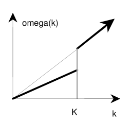
FIG. 1.: Schwinger’s model dispersion relation.

Note that the cut-off $K$ describes real physics: It is a surrogate for all the complicated physics that would be required to make a detailed model for the dielectric to vacuum transition in the dispersion relation.

Of course, this can all be recast in terms of a wave-number dependent refractive index

$${1\over n(k)}\equiv{\omega(k)\over c\;k},$$ (17)

and then, an integration by parts yields

$$E_{Casimir} = {V\hbar\over 6\pi^{2}}\int d(k^{3})\;[\omega(k)-ck]$$ (18)

$$= {V\hbar\over 6\pi^{2}}\Bigg{[}\left.\left(k^{3}\;[\omega(k)-ck]\right)\right|_{0}^{\infty}$$ (20)

$$\qquad-\int[d\omega(k)-d(ck)]k^{3}\Bigg{]}.$$

The boundary term vanishes because of the asymptotic behavior of $\omega(k)$, and the two substitutions $k=\omega(k)n/c$ and $k=\omega/c$ then give

$$E_{Casimir}=+{V\hbar\over 6\pi^{2}c^{3}}\int_{0}^{\infty}\omega^{3}[1-n^{3}(\omega)]d\omega.$$ (21)

In terms of the refractive index, of course, Schwinger’s model for the dispersion relation becomes (see figure 2)

$$n(k)=n\;\Theta(K-k)+\Theta(k-K),$$ (22)

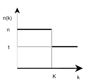
FIG. 2.: Schwinger’s model for the refractive index. Refractive index as a function of wave-number.

and equivalently (see figure 3)

$$n(\omega)=n\;\Theta([Kc/n]-\omega)+\Theta(\omega-Kc).$$ (23)

We now go on to the more general case of two dielectric media.

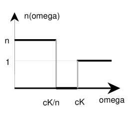
FIG. 3.: Schwinger’s model for the refractive index. Refractive index as a function of frequency.

B Two dielectric media

Suppose we now have two dielectrics to consider. We will deal with the situation where a dielectric body with dispersion relation $\omega_{1}(k)$ is embedded in an infinite slab of dielectric with dispersion relation $\omega_{2}(k)$. The total zero-point energy is easily written down

$$E_{embedded-body} = 2V\int{d^{3}\vec{k}\over(2\pi)^{3}}\;{1\over 2}\hbar\;\omega_{1}(k)$$ (24)

$$+ 2(V_{\infty}-V)\int{d^{3}\vec{k}\over(2\pi)^{3}}\;{1\over 2}\hbar\;\omega_{2}(k).$$ (25)

If the embedded body is removed, and the hole simply filled-in with the embedding medium, we can simply calculate the new total zero-point energy as

$$E_{homogeneous}=2V_{\infty}\int{d^{3}\vec{k}\over(2\pi)^{3}}\;{1\over 2}\hbar\;\omega_{2}(k).$$ (26)

We define the Casimir energy by subtracting these two zero-point energies

$$E_{Casimir} \equiv E_{embedded-body}-E_{homogeneous}$$ (27)

$$= 2V\int{d^{3}\vec{k}\over(2\pi)^{3}}\;{1\over 2}\hbar\;[\omega_{1}(k)-\omega_{2}(k)].$$ (28)

The physical import of this definition is clear: The Casimir energy is defined as the change in the zero-point energy due to a change in the medium.

From the general considerations in the previous subsection we know that the integrand must (still) go to zero at large wave-number, and in fact, for any pair of real physical dielectrics the integrand must go to zero sufficiently rapidly to make the integral converge.

The integration by parts discussed above can now be extended to yield

$$E_{Casimir}=+{V\hbar\over 6\pi^{2}c^{3}}\int_{0}^{\infty}\omega^{3}[n_{2}^{3}(\omega)-n_{1}^{3}(\omega)]d\omega.$$ (29)

While the difference between the refractive indices in the above expression goes to zero sufficiently rapidly to make the integral converge, it must be noted that the prefactor of $\omega^{3}$ implies that the net Casimir energy will be relatively sensitive to the high frequency behavior of the refractive indices.

If we now use Schwinger’s simple wave-number cut-off, we find that

$$E_{Casimir}={1\over 8\pi^{2}}V\;\hbar c\;\left\{K_{1}^{4}\left[{1\over n_{1}}-1\right]-K_{2}^{4}\left[{1\over n_{2}}-1\right]\right\}.$$ (30)

Notice that depending on the precise values of the two refractive indices and the two cut-offs, we can easily change the sign of the Casimir energy.

In particular, if we have a cavity containing vacuum embedded in an otherwise uniform dielectric $n_{1}=1$, and can for simplicity take $n_{2}=n$ and $K_{2}=K$, in which case

$$E_{Casimir}=-{1\over 8\pi^{2}}V\;\hbar c\;K^{4}\left[{1\over n}-1\right].$$ (31)

Note that this is exactly the negative of the result for a dielectric body embedded in vacuum. [See Eq. (16).] This observation serves to drive home the fact that the Casimir energy makes no sense until one has carefully specified the two physical situations whose energy difference is being calculated.

C A general cut-off

In order to appreciate the degree to which Schwinger’s expression is generic, notice that the dispersion relation can always be written in the form

$$\omega(k)=ck+ck\left[{1\over n}-1\right]{\cal F}(k/K).$$ (32)

This expression serves to define the function ${\cal F}(k/K)$, and the cut-off scale $K$. We know from the general discussion that ${\cal F}(0)=1$, while ${\cal F}(\infty)=0$. It is convenient to normalize $\cal F$ by ${\cal F}(1)=1/2$, and thus implicitly fix $K$ by the requirement that $\omega(K)=cK(n+1)/(2n)$. With this notation $K$ is the wave-number at which $\omega(k)/k$ has fallen half-way from its low-momentum dielectric value to its high wave-number free-space value. (See figure 4.)

FIG. 4.: Generic model dispersion relation.

In terms of the wave-number dependent refractive index,

$${1\over n(k)}=1+\left[{1\over n}-1\right]{\cal F}(k/K).$$ (33)

The Casimir energy difference is now simply written as

$$E_{Casimir}={1\over 2\pi^{2}}V\;\hbar c\;K^{4}\left[{1\over n}-1\right]\int_{0}^{\infty}x^{3}{\cal F}(x)dx.$$ (34)

This extension of Schwinger’s result makes manifest the salient points of the Casimir energy in dielectrics:
(1) The (dominant) contribution to the Casimir zero-point-energy is a bulk effect proportional to the volume of the displaced dielectric,
(2) and equivalently, the bulk Casimir energy density is

$$\rho={1\over 2\pi^{2}}\hbar c\;K^{4}\left[{1\over n}-1\right]\int_{0}^{\infty}x^{3}{\cal F}(x)dx.$$ (35)

(3) The dependence on refractive index at low momentum is explicitly known.
(4) There is an explicit ultraviolet cut-off $K$, and the Casimir energy is proportional to this cut-off to the fourth power—this cut-off is real physics, and is not an artifact to be renormalized away.
(5) It is only an accident of history that many, but by no means all, of the early Casimir effect calculations were for configurations where the cut-off dependence happens to vanish. (See [16].)
(6) There is an overall dimensionless constant that arises from the detailed behavior of the dispersion relation as a function of wave-number—this remaining overall factor cannot be calculated without developing a specific detailed model for the dispersion.
(7) The key physical insight underlying the Casimir effect is that the presence of a dielectric or conductor changes the photon dispersion relation and thereby changes the total zero-point energy.

If we wish to tackle the problem of one dielectric embedded in another, the relevant generalizations are clear: we simply write down individual cut-off functions ${\cal F}_{(1,2)}$ and cut-off scales $K_{(1,2)}$ for each dielectric. The Casimir energy difference is now given by

$$E_{Casimir} = {1\over 2\pi^{2}}V\;\hbar c\;\Bigg{\{}K_{1}^{4}\left[{1\over n_{1}}-1\right]\int_{0}^{\infty}x^{3}{\cal F}_{1}(x)dx$$ (37)

$$\qquad\qquad-K_{2}^{4}\left[{1\over n_{2}}-1\right]\int_{0}^{\infty}x^{3}{\cal F}_{2}(x)dx\Bigg{\}}.$$

Next we turn to a discussion of the finite-volume effects.

D Finite-volume effects

We now look at contributions arising from sub-dominant finite-volume corrections to the density of states. The key observation here is that the existence of finite-volume corrections proportional to the surface area of the dielectric is a generic result. The fact that Milton et al. encountered a surface-tension term proportional to $(\hbox{cut-off})^{3}$ is hereby explained on general physical grounds without recourse to special function theory.

Now, the fact that the dominant contribution to the Casimir energy is proportional only to volume is of course, merely a reflection of the fact that the canonical bulk expression for the density of states is proportional to volume: $\hbox{[Volume]}\,d^{3}\vec{k}/(2\pi)^{3}$. It is reasonably well-known, though perhaps not so elementary, that the density of states is in general modified by finite volume effects. Thus in general we should write

$$\sum_{n}\sim V\int{d^{3}\vec{k}\over(2\pi)^{3}}+S\int\xi{d^{3}\vec{k}\over(2\pi)^{3}k}+\cdots$$ (39)

These are the first two terms in an asymptotic expansion in $1/k$. A discussion of the general existence of such terms can be found in the textbook by Pathria [14], while a more extensive discussion has been given in the paper by Balian and Bloch [15]. For Dirichlet, von Neumann, and Robin boundary conditions the dimensionless variable $\xi$ is a known function of the boundary conditions imposed. For dielectric junction conditions, the case of interest in the current problem, the situation is considerably more complicated and will be dealt with in a forthcoming paper. For now we just point out that, introducing separate quantities $\xi_{in}$ and $\xi_{out}$ for the density of states inside and outside the dielectric body, the first finite-volume contribution to the Casimir energy is of the form

$$S\int{d^{3}\vec{k}\over(2\pi)^{3}k}\hbar\left[\xi_{in}\;\omega_{in}(k)+\xi_{out}\;\omega_{out}(k)\right],$$ (40)

that is to say

$$S\int{d^{3}\vec{k}\over(2\pi)^{3}}\hbar c\left[{\xi_{in}\over n_{in}(k)}+{\xi_{out}\over n_{out}(k)}\right].$$ (41)

For a simple wave-number cut-off, á la Schwinger, this becomes

$${1\over 6\pi^{2}}SK^{3}\hbar c\left[{\xi_{in}\over n_{in}}+{\xi_{out}\over n_{out}}\right],$$ (42)

which turns out to be in full agreement with the results enunciated in [10, 11, 12]. To actually complete the calculation we need to evaluate both $\xi_{in}$ and $\xi_{out}$ as functions of refractive index for both TE and TM modes. This will be the subject of a forthcoming paper [8].

E A potential source of confusion

A potential source of confusion should now be noted before it leads to trouble: If we introduce a naive cut-off in frequency (energy) rather than wave-number (three-momentum) then the Casimir zero-point energy appears to have a different behavior as a function of refractive index. This is merely a reflection of the fact that frequency cut-offs are in general ill-behaved, commonly leading to multi-branched dispersion relations.

For definiteness, consider what at first sight would seem to be the frequency cut-off version of Schwinger’s model

$$k(\omega)={n\omega\over c}\;\Theta(\omega_{0}-\omega)+{\omega\over c}\;\Theta(\omega-\omega_{0}).$$ (43)

Here $\Theta(x)$ is again the Heaviside step function, while $\omega_{0}$ is now a frequency which characterizes the transition from dielectric-like behavior to vacuum-like behavior. (See figure 3.) If we try to invert this function to obtain the dispersion relation $\omega(k)$, we see that it is double-valued in the range $k\in[\omega_{0}/c,n\omega_{0}/c]$. Momenta in this range will be doubly-counted, and lead to unphysical results. (See figure 5.)

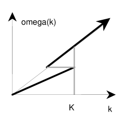
FIG. 5.: A naive frequency cut-off for the model dispersion relation: Note the unphysical double-valued nature of the dispersion.

For this particular model, we get

$$E_{Casimir}={1\over 8\pi^{2}}V\hbar c\left({\omega_{0}\over c}\right)^{4}\left[n^{3}-1\right].$$ (44)

Note that the double-counting has been sufficient to change the sign of the bulk Casimir energy! (See eq. (12)). Physically, the sign as determined in Schwinger’s calculation is the correct one as can be seen from a general argument: Suppose only that the dispersion relation is single-valued and that $\omega(k)<ck$, (equivalently $n(k)>1$), then the sign as determined by Schwinger is correct.

The $[n^{3}-1]$ behavior encountered above is in fact generic for frequency-based or energy-based cut-offs. In particular, (as we shall see below) if we impose point-slitting in time as our regulator, and then define energy differences by subtracting two time-split energies which are time-split at the same physical time, then we are effectively imposing a frequency-based regulator and will obtain the $[n^{3}-1]$ behavior. On the other hand, if we time-split using “optical time”, the parameter $\tau_{optical}=\tau_{physical}/n$, then we are effectively imposing a wave-number-based regulator, and we generically get a $[(1/n)-1]$ behavior.

A wave-number based regulator, following Schwinger’s prescription, is by far more physical than a naive frequency-based regulator. The only reason we belabor this point is because many calculations are carried out using naive time-splitting in physical time, and should be slightly modified (so that we time-split in optical time) before being compared to Schwinger’s result. Otherwise one is led into meaningless results.

We emphasize that this is a minor side issue that does not affect issues of volume dependence versus surface dependence, and thus does not alter the cut-off dependence. At worst these technical issues influence the behavior as a function of refractive index, and even then the order ($O[n-1]$) of the Casimir energy for dilute media ($n\approx 1$) will not be affected.

III Physical description of the calculations and existence of the volume term

The calculations presented by Milton et al. [10, 11, 12] avoid the density-of-states point of view by explicitly calculating the eigen-modes (equivalently, Green functions) for a specific model configuration: a dielectric ball (of dielectric constant $\epsilon_{1}$ and permeability $\mu_{1}$) embedded in an infinite slab of (different) dielectric constant $\epsilon_{2}$ and permeability $\mu_{2}$. They then explicitly integrated over these eigen-modes to calculate the Casimir energy.

Note that an important limitation of any such calculation is that while the density-of-states argument applies to dielectrics of arbitrary shape, any attempt at explicitly calculating eigen-modes must be restricted to systems of extremely high symmetry—such as for example half-spaces, slabs, or spheres.

The basic strategy is to start with the classical expression for the energy (where we have assumed that $\epsilon$ and ${\mu}$ are frequency independent constants)

$$E = {1\over 2}\int_{Geometry}d^{3}\vec{x}\left[\epsilon\vec{E}^{2}+{1\over\mu}\vec{B}^{2}\right].$$ (45)

We now promote the electric and magnetic fields to be operator quantities, and calculate the vacuum expectation value

$$E={1\over 2}\int_{Geometry}d^{3}\vec{x}\big{[} \epsilon \langle\vec{E}(0,\vec{x})\cdot\vec{E}(0,\vec{x})\rangle$$ (46)

$$+ {1\over\mu} \langle\vec{B}(0,\vec{x})\cdot\vec{B}(0,\vec{x})\rangle\big{]}.$$ (47)

The geometry is incorporated in the calculation both via the limits of integration and the boundary conditions satisfied by the fields. Since the above two-point functions are of course divergent, they must be rendered finite by some regularization prescription. Milton et al. use time-splitting (point-splitting in the time direction), defining the quantity $E(\tau)$ by:

$$E(\tau)={1\over 2}\int_{Geometry}d^{3}\vec{x}\big{[} \epsilon \langle\vec{E}(\tau,\vec{x})\cdot\vec{E}(0,\vec{x})\rangle$$ (48)

$$+ {1\over\mu} \langle\vec{B}(\tau,\vec{x})\cdot\vec{B}(0,\vec{x})\rangle\big{]}.$$ (49)

It should be pointed out that while time-splitting is a very powerful and technically useful ultra-violet regulator it has the decided disadvantage of obscuring the underlying physical basis of the cut-off in dielectric media.

The technical aspects of the analysis carried out by Milton et al. reduce then to calculating these two-point correlation functions (Green functions) by explicitly solving for the TE and TM modes appropriate for a spherical ball with dielectric boundary conditions. These Green functions can be written as a sum over suitable combinations of Ricatti–Bessel functions and vector spherical harmonics.

To avoid unnecessary notational complications, we schematically rewrite the above as

$$E(\tau)={1\over 2}\int d^{3}\vec{x}G_{[\epsilon,\mu]}(\tau,\vec{x};0,\vec{x}),$$ (50)

where $G_{[\epsilon,\mu]}(t,\vec{x};t^{\prime},\vec{x}^{\prime})$ is simply shorthand for the linear combination of Green functions appearing above.

These Green functions should be calculated for three different geometries:
Case I: A dielectric ball of dielectric constant $\epsilon_{1}$, permeability $\mu_{1}$, and radius $R$ embedded in a infinite dielectric of different dielectric constant $\epsilon_{2}$ and permeability $\mu_{2}$. (In applications to sonoluminescence, think of this as an air bubble of radius $R$ in water.)
Case II: A completely homogeneous space completely filled with dielectric $(\epsilon_{2},\mu_{2})$. (In applications to sonoluminescence, think of this as pure water.)
Case III: A completely homogeneous space completely filled with dielectric $(\epsilon_{1},\mu_{1})$. (In applications to sonoluminescence, think of this as pure air.)

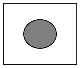
FIG. 6.: Case I: Dielectric ball (foreground) in dielectric background.

FIG. 7.: Case II: Homogeneous dielectric background.

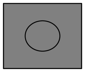
FIG. 8.: Case III: Homogeneous dielectric foreground.

We are in complete agreement with the extant calculations and results for these three individual Green functions—where we do not agree, as will be shown, is in the way that these three Green functions are inserted into the computation for the Casimir energy.

Milton et al. calculate an “energy difference”, which we will call $E_{surface}$, and which they define as

$$E_{surface}={1\over 2}\left\{\int_{all~{}space}G_{I}-\int_{r>R}G_{II}-\int_{r<R}G_{III}\right\}.$$ (51)

The computation of this quantity is mathematically correct—unfortunately this is simply not the physically correct quantity to be computing, and this definition is equivalent to explicitly excluding by hand the dominant volume contribution.

The appropriate physical quantity to compute is [1]

$$E_{Casimir}={1\over 2}\left\{\int_{all~{}space}G_{I}-\int_{all~{}space}G_{II}\right\}.$$ (52)

Observe that this quantity is simply the difference in energy between two situations: (Case I) having the dielectric ball present and (Case II) replacing the dielectric ball by the surrounding medium. This is exactly the quantity that Schwinger calculates in reference [1]. Within the context of sonoluminescence this is the Casimir energy released in evolving from bubble to no-bubble. In contrast, the definition of $E_{surface}$ above is not a physical difference between any two real physical situations. Rather it is a doubly subtracted quantity which does not respect the boundary conditions for the problem it tries to solve. In particular, $E_{surface}$ is not physically the same quantity as that calculated by Schwinger.

If we look at the difference between the appropriate definition (Schwinger’s) and that of Milton et al. we see that

$$\Delta E = E_{Casimir}-E_{surface}$$ (53)

$$= {1\over 2}\int_{r<R}\left\{G_{III}-G_{II}\right\}.$$ (54)

This difference is now easily seen to be the missing volume term: Remember that $G_{III}$ and $G_{II}$ are Green functions corresponding to spaces completely filled with homogeneous dielectrics—therefore these Green functions are translation invariant. (When we express these Green functions in terms of spherical polar coordinates it is not obvious that they are translation invariant, but because the physical dielectric in Cases II and III is translation invariant, the Green functions must also be translation invariant.) This observation permits us to pull the Green functions outside the integral, so that

$$\Delta E={1\over 2}V\left\{G_{III}(\tau,\vec{0};0,\vec{0})-G_{II}(\tau,\vec{0};0,\vec{0})\right\}.$$ (55)

This explicitly shows that the term omitted in the analyses of Milton et al. is a volume term. As we show below, it is in fact exactly the term required to bring that calculation into conformity with Schwinger’s result.

We shall show this by computing the difference term in two separate ways: (1) using translation invariance, dimensional analysis, conformal symmetry, and elementary quantum field theory it is possible to calculate this difference term from first principles for arbitrary geometries, and (2) particularizing to the case of a spherical dielectric ball, and working in spherical polar coordinates, we shall use Milton et al.’s own formulae for these Green functions and give an explicit expression for this difference as a sum over integrals involving Ricatti–Bessel functions. These integrals and sums will be evaluated explicitly in closed form, and we shall explicitly see how the correct volume, cut-off, and dielectric dependence emerge from the calculation.

IV An elementary quantum field theory calculation

To evaluate the time-split energy density we apply some standard results from flat-space Minkowski quantum field theory. Note that in the Feynman gauge, the two-point function for the electromagnetic vector potential is given by

$$\langle T(A_{\mu}(x)A_{\nu}(y))\rangle = {\hbar\over(2\pi)^{2}}{\eta_{\mu\nu}\over(x-y)^{2}}$$ (56)

$$= {\hbar\over(2\pi)^{2}}{\eta_{\mu\nu}\over c^{2}[t(\vec{x})-t(\vec{y})]^{2}-(\vec{x}-\vec{y})^{2}},$$ (57)

and for the Minkowski vacuum

$$\langle\vec{E}(\tau,\vec{x})\cdot\vec{E}(0,\vec{x})\rangle=\langle\vec{B}(\tau,\vec{x})\cdot\vec{B}(0,\vec{x})\rangle={\hbar\over(2\pi)^{2}}{12\over(c\tau)^{4}}.$$ (58)

The (regulated) vacuum energy is simply [cf. eq. (48)]

$$E(\tau)_{vacuum}={\hbar\over(2\pi)^{2}}\;V\;{12\over(c\;\tau)^{4}}.$$ (59)

However, the effect of adding a frequency independent dielectric constant, can be simply mimicked by re-scaling the physical metric $\eta_{\mu\nu}$, thereby introducing what we shall call the “optical metric”

$$g_{\mu\nu}^{optical}={\rm diag}[+1/n^{2},-1,-1,-1];$$ (60)

$$g^{\mu\nu}_{optical}={\rm diag}[+n^{2},-1,-1,-1].$$ (61)

Note that on-shell photons in the dielectric will travel along null curves of this optical metric. The introduction of this optical metric is a nice technical trick for dealing with homogeneous and non-dispersive dielectrics by means of viewing them as special deformations of Minkowski space.

In terms of this optical metric we can still write

$$E(\tau)^{optical}_{dielectric}={\hbar\over(2\pi)^{2}}\;V_{optical}\;{12\over(c\;\tau_{optical})^{4}}.$$ (62)

This energy is to be interpreted as that which would be measured by a hypothetical observer for whom the optical metric would be physical. This energy must be translated back to physical quantities by means of the following equivalences:

$$E_{physical} = E_{optical}/n;$$ (63)

$$\tau_{physical} = \tau_{optical}\;n;$$ (64)

$$V_{physical} = V_{optical}.$$ (65)

The effect of these translations is that the time-split energy density (time-split in physical time) becomes

$$E(\tau_{physical})^{physical}_{dielectric}={\hbar\over(2\pi)^{2}}V_{physical}\;n^{3}{12\over(c\;\tau_{physical})^{4}}.$$ (66)

But, on the other hand, time-splitting in optical time yields

$$E(\tau_{optical})^{physical}_{dielectric}={\hbar\over(2\pi)^{2}}V_{physical}\;{1\over n}\;{12\over(c\;\tau_{optical})^{4}}.$$ (67)

This now permits us to evaluate exactly the missing piece that Milton et al. discarded; with the convention of time-splitting in physical time, that term is

$$\Delta E^{physical}_{fixed~{}{\tau_{physical}}}$$ (68)

$$\qquad\qquad=E(\tau_{physical})^{physical}_{dielectric~{}1}-E(\tau_{physical})^{physical}_{dielectric~{}2}$$ (69)

$$\qquad\qquad={\hbar\over(2\pi)^{2}}V_{physical}\;[n_{1}^{3}-n_{2}^{3}]\;{12\over(c\;\tau_{physical})^{4}}.$$ (70)

Since Milton et al. express all their results in spherical polar coordinates, as sums over an infinite number of Ricatti–Bessel functions, it is far from obvious that the rather formidable expressions encountered in those analyses reduce to the simple and exact result displayed above. In the next section of this paper we will do exactly this by invoking a long and turgid agony of special function theory.

Before leaving this section, however, we wish to emphasize that comparing this result to the original Schwinger calculation requires one additional modification: Schwinger regulated his energy calculation by introducing a cut-off at fixed wave-number (three-momentum). This is equivalent to time-splitting at fixed optical time. To see this, recall that frequency and wave-number cut-offs are in a non-dispersive dielectric related by

$$n\omega_{0}=cK,$$ (71)

in which case

$$\tau_{physical}\sim 1/\omega_{0},$$ (72)

while on the other hand

$$\tau_{optical}={\tau_{physical}\over n}\sim{1\over n\omega_{0}}={1\over cK}.$$ (73)

Thus, if we regularize by time-splitting, and perform the subtraction at fixed optical time, we have

$$\Delta E^{physical}_{fixed~{}{\tau_{optical}}}$$ (74)

$$\qquad\qquad=E(\tau_{optical})^{physical}_{dielectric~{}1}-E(\tau_{optical})^{physical}_{dielectric~{}2}$$ (75)

$$\qquad\qquad={\hbar\over(2\pi)^{2}}V_{physical}\left[{1\over n_{1}}-{1\over n_{2}}\right]{12\over(c\;\tau_{optical})^{4}}.$$ (76)

This is exactly Schwinger’s result as enunciated in [1]. (More precisely, it is as close as one is ever going to get considering that a sharp cut-off is just not the same as time-splitting: There is no reason to expect the dimensionless coefficients to be the same for the two calculations. We will comment, near the end of the next section, how we can switch from a time splitting cut-off to a sharp cut-off in wave number and obtain exactly Schwinger’s coefficient.)

In summary, what we have shown achieved so far is to show the following:

(1) Schwinger’s calculation [1] showing that there is a bulk Casimir energy in a generic dielectric is correct.

(2) The analyses of Milton et al. [10, 11, 12] omit the volume contribution to the Casimir energy.

(3) The volume contribution that was omitted in those analyses can be calculated exactly, without resorting to special function theory or asymptotic analysis, and the omitted term exactly reproduces the volume contribution as evaluated by Schwinger.

(4) The volume term in the calculation was missed because of misidentification of a Green function, due to the incorrect application of boundary conditions.

(5) This argument is not limited to systems of spherical symmetry. From the preceding it is clear that the argument continues to hold for arbitrarily shaped dielectrics.

In the next section we will evaluate $\Delta E$ given in eq. (54) in yet a different way: by working directly from Milton’s expression.

V The energy difference term in spherical coordinates

From the preceding discussion we have isolated the term in the Casimir energy that Milton et al. [10, 11, 12] omitted. It is precisely the difference between the Green functions (of Case III and Case II) integrated over the interior of the bubble (See eq. (54)). We can thus immediately jump into the middle of the technical computation and directly evaluate this difference term. This calculation has the advantage of quickly getting to the heart of the matter.

From the two recent papers [11], eq. (41), or from [12], eq. (4.2b), we can write

$$\Delta E = E_{Casimir}-E_{surface}$$ (77)

$$= {\rm Re}\bigg{\{}{-i\over 2}\int_{-\infty}^{+\infty}{d\omega\over 2\pi}e^{-i\omega\tau}\int_{0}^{R}r^{2}dr$$ (79)

$$\qquad\times\left[\tilde{X}_{III}(k_{III},r)-\tilde{X}_{II}(k_{II},r)\right]\bigg{\}}.$$

Here we use the notation $k=|\omega|n$, with $n$ the appropriate refractive index, and define the quantity $\tilde{X}_{II}(k_{II},r)$ by

$$\tilde{X}_{II}(k_{II},r) \equiv \sum_{\ell=1}^{\infty}(2\ell+1)\Bigg{\{}2\;k_{II}^{2}\;F^{II}_{\ell}(k_{II};r,r)+$$ (82)

$$+{1\over r^{2}}{\partial\over\partial r}\left[r{\partial\over\partial r^{\prime}}r^{\prime}\left[F^{II}_{\ell}(k_{II};r,r^{\prime})\right]\Big{|}_{r^{\prime}=r}\right]\Bigg{\}}$$

$$+\left[(F_{\ell}^{II})\to(G_{\ell}^{II})\right].$$

The $F_{\ell}$ and $G_{\ell}$ Green functions are identical to those in [10, 11, 12]. Notice that when making the substitution $(II)\to(III)$ we should also change the refractive index that implicitly appears in the factor $k$.

In writing these equations we have used the fact that the energy difference is known to be a real quantity, so we can immediately discard the imaginary part of the above expression without bothering to explicitly evaluate it. There is no subtle physics involved here—this is just the standard procedure of using complex exponentials to represent a harmonic time dependence and then taking the real part at the end of the calculation. In particular there is no physics hiding in the imaginary part of the above expression. Not only is there no need to calculate the imaginary part, but it is physically meaningless to do so.

If we were integrating over all space, then — following [10, 11, 12] — the partial derivative terms in ${\tilde{X}}(k,r)$ could be safely dropped. Because we are only integrating over a finite region we must explicitly keep these derivative terms.

Now because $k=|\omega|n$, while $F_{\ell}$ and $G_{\ell}$ are functions of $k$, they are therefore functions only of the absolute value of $\omega$. This permits us to write

$$\Delta E = {\rm Re}\bigg{\{}{-i\over 2}\int_{0}^{+\infty}{d\omega\over 2\pi}\left[e^{-i\omega\tau}+e^{+i\omega\tau}\right]$$ (84)

$$\qquad\times\int_{0}^{R}r^{2}dr\left[\tilde{X}_{III}(k_{III}r)-\tilde{X}_{II}(k_{II}r)\right]\bigg{\}}.$$

$$= {\rm Re}\bigg{\{}{-i}\int_{0}^{+\infty}{d\omega\over 2\pi}\cos(\omega\tau)\;$$ (86)

$$\qquad\times\int_{0}^{R}r^{2}dr\;\left[\tilde{X}_{III}(k_{III}r)-\tilde{X}_{II}(k_{II}r)\right]\bigg{\}},$$

and finally

$$\Delta E = \int_{0}^{+\infty}{d\omega\over 2\pi}\cos(\omega\tau)\;\int_{0}^{R}r^{2}dr\;$$ (88)

$$\times{\rm Im}\ \left[\tilde{X}_{III}(k_{III},r)-\tilde{X}_{II}(k_{II},r)\right].$$

The Green functions for Cases II and III are very simple (since we are dealing with homogeneous spaces) and the imaginary parts can easily be read off from [10] eq. (29), [11] eq. (35), or [12] eq. (3.7)

$${\rm Im}\{F_{\ell}\}={\rm Im}\{G_{\ell}\} = {\rm Im}\{ik\;j_{\ell}(k,r)\;h_{\ell}(kr)\}$$ (90)

$$= k\;j_{\ell}^{2}(kr)$$ (91)

$$= k\;{s_{\ell}^{2}(kr)\over(kr)^{2}}.$$ (92)

Here we have introduced the Ricatti–Bessel function $s_{\ell}(x)$. (We refer the reader to the Appendix for details.) Inspection of the derivative pieces yields

$${\rm Im}\left\{{\partial\over\partial r}\left[r{\partial\over\partial r^{\prime}}r^{\prime}\left[F_{\ell}(k;r,r^{\prime})\right]\Big{|}_{r^{\prime}=r}\right]\right\}$$ (93)

$$\qquad={\rm Im}\left\{{\partial\over\partial r}\left[r{\partial\over\partial r^{\prime}}r^{\prime}\left[G_{\ell}(k;r,r^{\prime})\right]\Big{|}_{r^{\prime}=r}\right]\right\}$$ (94)

$$\qquad={\rm Im}\big{\{}ik\;\big{[}(xh_{\ell}(x))^{\prime}|_{kr}\;(xj_{\ell}(x))^{\prime}|_{kr}$$ (95)

$$\qquad\qquad+(xh_{\ell}(x))|_{kr}\;(xj_{\ell}(x))^{\prime\prime}|_{kr}\big{]}\big{\}}$$ (96)

$$\qquad=k\;{\rm Re}\{e_{\ell}^{\prime}(x)|_{kr}\;s_{\ell}^{\prime}(x)|_{kr}+e_{\ell}(x)|_{kr}\;s_{\ell}^{\prime\prime}(x)|_{kr}\}$$ (97)

$$\qquad=k\;\{s_{\ell}^{\prime}(x)|_{kr}\;s_{\ell}^{\prime}(x)|_{kr}+s_{\ell}(x)|_{kr}\;s_{\ell}^{\prime\prime}(x)|_{kr}\},$$ (98)

with $e_{\ell}(x)$ another Ricatti-Bessel function.

To derive these results we can either use brute force starting from eq. (35) of [11], or alternatively we could inspect equations (19–22) of [10]. (Note that there was an overall change in normalization between the 1980 paper and the 1995 and 1996 papers, and take account of the fact that we are here retaining the total derivative term.)

All together, this implies

$${\rm Im}\left[\tilde{X}_{III}(k_{III},r)-\tilde{X}_{II}(k_{II},r)\right]$$ (99)

$$=2\;{k_{III}\over r^{2}}\;\sum_{\ell=1}^{\infty}(2\ell+1)$$ (100)

$$\times\left\{2(s_{\ell}(x))^{2}+([s_{\ell}(x)]^{\prime})^{2}+s_{\ell}(x)s_{\ell}^{\prime\prime}(x)\right\}|_{k_{III}r}$$ (101)

$$-[(III)\to(II)].$$ (102)

The sum over Ricatti–Bessel functions is now easily and exactly evaluated using the results in the Appendix. We simply get

$${\rm Im}\{\tilde{X}_{III}(k_{III},r)-\tilde{X}_{II}(k_{II},r)\} = 2\;\left[{k\over r^{2}}\;2(kr)^{2}\right]\Big{|}^{(III)}_{(II)}$$ (103)

$$= 4\left[k_{III}^{3}-k_{II}^{3}\right]$$ (104)

$$= 4\left[n_{1}^{3}-n_{2}^{3}\right]|\omega|^{3}.$$ (105)

Notice that the above expression is independent of $r$ —a result that is by no means obvious from the original definition. (But we knew from the fact that the underlying Green functions are translation invariant that this quantity had to be independent of position at the end of the day!)

Turning again to the energy difference

$$\Delta E=\left[n_{1}^{3}-n_{2}^{3}\right]\int_{0}^{+\infty}{d\omega\over 2\pi}\left[\cos(\omega\tau)\right]\int_{0}^{R}r^{2}dr\;4\omega^{3}.$$ (106)

Which is now easily evaluated, using $x=\omega\tau$, as

$$\Delta E={2\over 3\pi}\left[n_{1}^{3}-n_{2}^{3}\right]\;{R^{3}\over\tau^{4}}\int_{0}^{+\infty}x^{3}\cos(x)dx.$$ (107)

As a penultimate step we use

$$\int_{0}^{+\infty}x^{3}\cos(x)dx=6,$$ (108)

and $V=(4\pi/3)R^{3}$, to write

$$\Delta E={3\over\pi^{2}}\left[n_{1}^{3}-n_{2}^{3}\right]{1\over\tau^{4}}\;V.$$ (109)

Re-inserting factors of $\hbar$ and $c$, which have been suppressed for clarity, we see

$$\Delta E(\tau_{physical})={3\over\pi^{2}}\;\hbar c\;\left[n_{1}^{3}-n_{2}^{3}\right]{1\over(c\;\tau_{physical})^{4}}\;V.$$ (110)

Note that this is exactly the same result (including numerical coefficients) as the previously calculated from general considerations using translation invariance and the strategy of introducing the optical metric. [See eq. (70).]

Finally, as discussed previously, we note that to compare this result to Schwinger’s we should be time-splitting in optical time, and so must absorb a few factors of refractive index into the time-splitting parameter. [See eq. (76).]

$$\Delta E(\tau_{optical})={3\over\pi^{2}}\;\hbar c\;\left[{1\over n_{1}}-{1\over n_{2}}\right]{1\over(c\;\tau_{optical})^{4}}V.$$ (111)

This is exactly the time-split version of Schwinger’s expression (70) for the bulk contribution to the Casimir energy.

We have thus evaluated the difference term, $\Delta E=E_{Casimir}-E_{surface}$, in two independent and completely independent ways. The two calculations agree down to exact numerical coefficients. Turning this result around, we have

$$E_{Casimir}=\Delta E+E_{surface}.$$ (112)

So we see that the term we have just calculated provides the bulk volume contribution to the Casimir energy that is required to bring Milton et al.’s calculations into conformity with Schwinger’s arguments [1], and into conformity with the general arguments provided in this paper.

To finally compare the absolute normalization of this result with Schwinger’s, we must explicitly replace the time-splitting by a wave-number cut-off. Simply go back to eq. (88), introduce a wave-number cut-off, and let the time-splitting parameter go to zero, to obtain

$$\Delta E = \int_{0}^{+\infty}{d\omega\over 2\pi}\;\int_{0}^{R}r^{2}dr\;$$ (114)

$$\times{\rm Im}\{f(k_{III})\tilde{X}_{III}(k_{III},r)-f(k_{II})\tilde{X}_{II}(k_{II},r)\}.$$

The function $f(k)$ is any real smooth function with $f(0)=1$ and $f(+\infty)=0$. For simplicity we have temporarily used the same cut-off function for the two media. We generalize the argument below. The evaluation of the various pieces of the Green functions proceeds as before, so that eq. now (106) becomes

$$\Delta E=\int_{0}^{+\infty}{d\omega\over 2\pi}\int_{0}^{R}r^{2}dr4\{f(k_{III})k_{III}^{3}-f(k_{II})k_{II}^{3}\}.$$ (116)

After a change of variables, and an explicit evaluation of the volume integral, we easily get

$$\Delta E=\left[{1\over n_{1}}-{1\over n_{2}}\right]V\int{d^{3}\vec{k}\over(2\pi)^{3}}f(k)k.$$ (117)

Approximating air by vacuum, (i.e. setting $n_{1}=1$), and inserting a sharp cut-off at wave-number $K$, (by setting $f(k)=\Theta(K-k)$), this is exactly Schwinger’s bulk volume term for a cavity in a dielectric [eq. (31)] down to the last numerical prefactor.

Now the use of a single cut-off function, while mathematically more transparent, is physically dubious. If we introduce separate cut-off functions for the two media the modifications are straightforward. First

$$\Delta E = \int_{0}^{+\infty}{d\omega\over 2\pi}\;\int_{0}^{R}r^{2}dr\;$$ (119)

$$\times{\rm Im}\{f_{III}(k_{III})\tilde{X}_{III}(k_{III},r)-f_{II}(k_{II})\tilde{X}_{II}(k_{II},r)\}.$$

The functions $f_{a}(k)$ are now any two real smooth functions with $f_{a}(0)=1$ and $f_{a}(+\infty)=0$. We now have

$$\Delta E=\int_{0}^{+\infty}{d\omega\over 2\pi}\int_{0}^{R}r^{2}dr4\{f_{III}(k_{III})k_{III}^{3}-f_{II}(k_{II})k_{II}^{3}\}.$$ (121)

After a change of variables, setting $f_{III}=f_{1}$ and $f_{II}=f_{2}$, and explicit evaluation of the volume integral, we easily get

$$\Delta E=V\int{d^{3}\vec{k}\over(2\pi)^{3}}\left[{f_{1}(k)\over n_{1}}-{f_{2}(k)\over n_{2}}\right]k.$$ (122)

Inserting sharp cut-offs in wave-number, á la Schwinger, is accomplished by setting

$$f_{a}(k)=\left[\Theta(K_{a}-k)+n_{a}\Theta(k-K_{a})\right]\Theta(K_{\infty}-k).$$ (123)

These cut-off functions may look a little mysterious, depending as they do on three cut-off scales $K_{1}$, $K_{2}$, and $K_{\infty}$. The two cut-offs $K_{1}$ and $K_{2}$ are physical—they describe the wave-numbers at which the two dispersion relations effectively approach the vacuum dispersion relation. The third cut-off $K_{\infty}$ is purely a mathematical convenience to make the integrals converge. $K_{\infty}$ should be taken to be much larger than either $K_{1}$ or $K_{2}$. With this notation

$${ckf_{a}(k)\over n_{a}} = \left[{ck\over n_{a}}\Theta(K_{a}-k)+ck\Theta(k-K_{a})\right]\Theta(K_{\infty}-k)$$ (124)

$$= \omega_{a}(k)\Theta(K_{\infty}-k).$$ (125)

That is to say, these particular cut-off functions have been chosen to mimic the model dispersion relation used in the mode sum discussion (section II).

Evaluating the integrals, and reinserting factors of $\hbar$ and $c$, we can write

$$\Delta E={1\over 8\pi^{2}}V\;\hbar c\;\left\{K_{1}^{4}\left[{1\over n_{1}}-1\right]-K_{2}^{4}\left[{1\over n_{2}}-1\right]\right\}.$$ (126)

Note in particular that $K_{\infty}$ has quietly disappeared from this answer. This is exactly the same as the result obtained by mode sum arguments in section II down to the last numerical prefactor. [See eq. (30).]

A slightly more general cut-off is to use the wave-number dependent refractive index to construct the cut-off according to the scheme

$$f_{a}(k)=\left[{n_{a}(k=0)\over n_{a}(k)}\right]\Theta(K_{\infty}-k).$$ (127)

In which case, recalling that that $n_{a}=n_{a}(k=0)$

$${ckf_{a}(k)\over n_{a}}=\left[{ck\over n_{a}(k)}\right]\Theta(K_{\infty}-k)=\omega_{a}(k)\Theta(K_{\infty}-k).$$ (128)

The Casimir energy difference, including reinserted factors of $\hbar$ and $c$, is now

$$\Delta E=\hbar V\int{d^{3}\vec{k}\over(2\pi)^{3}}\left[\omega_{1}(k)-\omega_{2}(k)\right]\Theta(K_{\infty}-k).$$ (129)

We can now let $K_{\infty}$ tend to infinity, and thereby recover eq. (28).

In summary, the energy difference term calculated via explicit summation over Ricatti–Bessel functions is completely in agreement with the dominant volume term coming from simple mode sum and density of states arguments.

VI Full calculation from first principles

A Background

There is also a certain amount of value to going to the trouble of redoing the calculation from first principles.

Recall that the physical quantity that we are interested in evaluating for the calculation of the Casimir energy is the total energy. The total classical energy is computed from the integral of the energy density over the geometry,

$$E=\int_{Geometry}d^{3}\vec{x}\;\frac{1}{2}\;\left(\epsilon\vec{E}^{2}+\mu\vec{H}^{2}\right).$$ (130)

After quantization this energy is related to the vacuum expectation value of the squares of the electric and magnetic fields in the dielectric.

Since the electric and magnetic fields are related to derivatives of the electromagnetic potential, the energy density is calculable in terms of the two–point correlation function of the electromagnetic field; these correlators are in general divergent, and we need to perform renormalizations before comparing with the results of experiments. This, of course, is nothing but the general recipe for evaluating quantities in any quantum field theory.

This calculation has been done in detail by Milton et al. [10, 11, 12] for the geometrical configuration previously described. They computed the total energy $E$ by integrating the electromagnetic energy density over the geometry and then rendered the expressions finite using point-splitting regularization in the time direction. We quote the expressions from them (see below for the various definitions), as

$$E = {\rm Re}\Bigg{\{}\int d^{3}\vec{x}\;\frac{1}{2}\;\left(\epsilon\vec{E}^{2}+\mu\vec{H}^{2}\right)\Bigg{\}}$$ (131)

$$= {\rm Re}\Bigg{\{}\frac{1}{2i}\int_{-\infty}^{\infty}\frac{d\omega}{2\pi}e^{-i\omega(t-t^{\prime})}\sum_{l=1}^{\infty}(2l+1)$$ (134)

$$\qquad\times\int_{0}^{\infty}r^{2}dr\big{\{}2k^{2}[F_{\ell}(k;r,r)+G_{\ell}(k;r,r)]$$

$$\qquad\qquad+[{\rm Derivative\;\;Terms}]\big{\}}\Bigg{\}}.$$

Here the total derivative can be shown (Ref. 10 of Milton) to integrate to zero. In this equation the $\omega$–integral is for the regulator in the time–direction, and the radial functions $F_{\ell}(r,r^{\prime})$ and $G_{\ell}(r,r^{\prime})$ are related to the Green functions for the electric and magnetic fields in the appropriate geometry. For a dielectric sphere of radius $R$, permeability $\epsilon_{1}$ and permittivity $\mu_{1}$, embedded in another dielectric with $\epsilon_{2}$ and $\mu_{2}$, using the results of Boyer [17, 18] as adapted by Milton et al., it is possible to readily check that these objects are the radial part of the Green functions for the wave equation in spherical coordinates,

$$\left({\partial^{2}\over\partial r^{2}}+\frac{2}{r}{\partial\over\partial r}-\frac{\ell(\ell+1)}{r^{2}}+k^{2}\right)F_{\ell}(k;r,r^{\prime})$$ (135)

$$\qquad\qquad=-\frac{1}{r^{2}}\delta(r-r^{\prime}),$$ (136)

and are given explicitly as follows:

For $r,r^{\prime}<R$,

$$F_{\ell}(k_{in};r,r^{\prime}) = ik_{in}j_{\ell}(k_{in}r_{<})$$ (138)

$$\times[h_{\ell}(k_{in}r_{>})-A^{\ell}_{F}j_{\ell}(k_{in}r_{>})].$$

For $r,r^{\prime}>R$,

$$F_{\ell}(k_{out};r,r^{\prime}) = ik_{out}h_{\ell}(k_{out}r_{>})$$ (140)

$$\times[j_{\ell}(k_{out}r_{<})-B^{\ell}_{F}h_{\ell}(k_{out}r_{<})].$$

A similar expression holds for $G_{\ell}$. In these two expressions the wave numbers are $k_{in}=|\omega|\sqrt{\epsilon_{1}\mu_{1}}$ and $k_{out}=|\omega|\sqrt{\epsilon_{2}\mu_{2}}$. The function $j_{\ell}(x)$ is the spherical Bessel function of order $\ell$ and $h_{\ell}(x)\equiv h_{\ell}^{(1)}(x)$ is the spherical Hankel function of the first kind. The quantities $A^{\ell}_{F}$, $A^{\ell}_{G}$, $B^{\ell}_{F}$ and $B^{\ell}_{G}$, are given in [10, 11, 12] and their explicit forms are obtained by requiring that the Green functions be solutions to the appropriate equations satisfying the correct boundary conditions.

Milton et al. in their papers give the expression for the energy that we quote above, eq. (134), after they have integrated over all of space before subtracting the energies for each material configuration. This is dangerous since there is then an additional infrared divergence arising from the volume integral which is not regulated by the time splitting–procedure, which only regulates UV divergences. To avoid these unnecessary pitfalls we will write down the energy density, perform the subtractions at the level of the densities (local subtractions) and then integrate.

Using the spherical Bessel function form for the electric and magnetic fields satisfying the Maxwell equations, the energy density, $T^{tt}$, is seen to be given by

$$T^{tt}(r)={\rm Re}\bigg{\{}{-i\over 2}\int_{-\infty}^{+\infty}{d\omega\over 2\pi}e^{-i\omega\tau}\;X(k,r)\bigg{\}},$$ (141)

where we have used the notation $k=|\omega|n$ with $n$ the refractive index appropriate for the medium, and defined the quantity $X(k,r)$ via

$$X(k,r) \equiv \sum_{\ell=1}^{\infty}(2\ell+1)\Bigg{\{}\left[k^{2}+{\ell(\ell+1)\over r^{2}}\right]\left[F_{\ell}(k;r,r)\right]$$ (144)

$$+{1\over r^{2}}{\partial\over\partial r_{1}}r_{1}{\partial\over\partial r_{2}}r_{2}\left[F_{\ell}(k;r_{1},r_{2})\right]\Big{|}_{r_{1}=r_{2}=r}\Bigg{\}},$$

$$+[(F_{\ell})\to(G_{\ell})].$$

This is of course equivalent to eq. (134) above. Here $k_{I}\equiv|\omega|n_{I}$ represents the wave-number for light of frequency $\omega$ in a medium with index of refraction $n_{I}$. Similar results, with appropriate substitutions for the momenta and Green functions, hold for the situations when we make reference to Cases II and III. Note that when making the substitutions $(I)\to(II)$ or $(I)\to(III)$ we must also change the refractive index that implicitly appears in the factor $k$. In addition, it should be borne in mind that $k_{I}$ is a function of position: $k_{I}=n_{1}|\omega|=k_{III}$ inside the dielectric sphere, whereas $k_{I}=n_{2}|\omega|=k_{II}$ outside the dielectric sphere.

The Casimir energy is now obtained by taking the difference in energy densities and integrating over all of space while paying attention to the appropriate index of refraction for each region of space. For example, the Casimir energy difference between Cases I and II is given by

$$E_{Casimir} = {\rm Re}\bigg{\{}{-i\over 2}\int_{0}^{\infty}r^{2}dr\;\int_{-\infty}^{+\infty}{d\omega\over 2\pi}$$ (146)

$$\qquad\times e^{-i\omega\tau}X(k_{I},k_{II},r)\bigg{\}},$$

where we have defined the quantity $X(k_{I},k_{II},r)$ by

$$X(k_{I},k_{II},r) \equiv X_{I}(k_{I},r)-X_{II}(k_{II},r)$$ (147)

$$= \sum_{\ell=1}^{\infty}(2\ell+1)\Bigg{\{}\left[k_{I}^{2}+{\ell(\ell+1)\over r^{2}}\right]$$ (152)

$$\times\left[F^{I}_{\ell}(k_{I};r,r)+G^{I}_{\ell}(k_{I};r,r)\right]$$

$$+{1\over r^{2}}\;{\partial\over\partial r_{1}}r_{1}{\partial\over\partial r_{2}}r_{2}\big{[}F^{I}_{\ell}(k_{I};r_{1},r_{2})$$

$$\qquad+G^{I}_{\ell}(k_{I};r_{1},r_{2})\big{]}\Big{|}_{r_{1}=r_{2}=r}\Bigg{\}}$$

$$-\left[(I)\to(II)\right].$$

To turn this into eq. (41) of reference [11] requires a few technicalities which were not made explicit by Milton but we will show here. (Note that the above is his eq. (42) in the hep-th version of the paper.)

Observe that

$${\partial\over\partial r}\left[r{\partial\over\partial r^{\prime}}r^{\prime}\left[F^{I}_{\ell}(k_{I};r,r^{\prime})+G^{I}_{\ell}(k_{I};r,r^{\prime})\right]\Big{|}_{r^{\prime}=r}\right]$$ (153)

$$={\partial\over\partial r_{1}}r_{1}{\partial\over\partial r_{2}}r_{2}\left[F^{I}_{\ell}(k_{I};r_{1},r_{2})+G^{I}_{\ell}(k_{I};r_{1},r_{2})\right]\Big{|}_{r_{1}=r_{2}=r}$$ (154)

$$\qquad+r{\partial^{2}\over\partial r^{\prime 2}}r^{\prime}\left[F^{I}_{\ell}(k_{I};r,r^{\prime})+G^{I}_{\ell}(k_{I};r,r^{\prime})\right]\Big{|}_{r^{\prime}=r}$$ (155)

$$={\partial\over\partial r_{1}}r_{1}{\partial\over\partial r_{2}}r_{2}\left[F^{I}_{\ell}(k_{I};r_{1},r_{2})+G^{I}_{\ell}(k_{I};r_{1},r_{2})\right]\Big{|}_{r_{1}=r_{2}=r}$$ (156)

$$\qquad-\left[k_{I}^{2}-{\ell(\ell+1)\over r^{2}}\right]r^{2}\left[F^{I}_{\ell}(k_{I};r,r)+G^{I}_{\ell}(k_{I};r,r)\right]$$ (157)

$$\qquad-2\delta(0),$$ (158)

where in the last line we have used the differential eq. (136) satisfied by the Green functions to replace the double derivative at the same point by an explicit polynomial.

The term proportional to $\delta(0)$ arises from the source term on the RHS of the differential equation (136) defining the Green functions. Fortunately this term is completely independent of the dielectric properties and in fact is independent of all properties of the medium. Thus when calculating energy differences this term cancels identically. (Earlier calculations often quietly discard this term without even mentioning its existence.)

Inserting this into the general formula for the Casimir energy, eq. (146), yields eq. (41) of reference [11]. Explicitly, it allows us to re-write $X(k_{I},k_{II},r)$ as

$$X(k_{I},k_{II},r) \equiv \sum_{\ell=1}^{\infty}(2\ell+1)\Bigg{\{}2k_{I}^{2}\Big{[}F^{I}_{\ell}(k_{I};r,r)$$ (163)

$$\qquad\qquad+G^{I}_{\ell}(k_{I};r,r)\Big{]}$$

$$+{1\over r^{2}}\;{\partial\over\partial r}\Bigg{[}r{\partial\over\partial r^{\prime}}r^{\prime}\Big{[}F^{I}_{\ell}(k_{I};r,r^{\prime})$$

$$\qquad\qquad+G^{I}_{\ell}(k_{I};r,r^{\prime})\Big{]}\Big{|}_{r^{\prime}=r}\Bigg{]}\Bigg{\}}$$

$$-\left[(I)\to(II)\right],$$

which is now straightforward to evaluate.

We know that $k$ is only dependent on the absolute value of $\omega$, which permits us to write

$$E_{Casimir} = {\rm Re}\Bigg{\{}{-i\over 2}\int_{0}^{\infty}r^{2}dr\int_{0}^{+\infty}{d\omega\over 2\pi}\left[e^{-i\omega\tau}+e^{+i\omega\tau}\right]$$ (165)

$$\qquad\times X(k_{I},k_{II},r)\Bigg{\}}.$$

Wherefore

$$E_{Casimir} = {\rm Re}\Bigg{\{}{-i}\int_{0}^{\infty}r^{2}dr\;\int_{0}^{+\infty}{d\omega\over 2\pi}\cos(\omega\tau)\;$$ (167)

$$\qquad\times X(k_{I},k_{II},r)\Bigg{\}}.$$

We are thus led to

$$E_{Casimir} = \int_{0}^{\infty}r^{2}dr\;\int_{0}^{+\infty}{d\omega\over 2\pi}$$ (169)

$$\qquad\times\cos(\omega\tau)\;{\rm Im}\{X(k_{I},k_{II},r)\}.$$

With due caution, the relevant pieces of the Green functions can be read off from [10, 11, 12].

B Calculation of the various Green functions.

The general form of the Green functions were given above, but one must require that the boundary conditions appropriate to the geometry and the physics be correctly incorporated into them. This means that they must satisfy appropriate continuity conditions derived from Maxwell’s equations. In terms of the fields,

$$\vec{E}_{\perp},\quad\epsilon\vec{E}_{r},\quad{1\over\mu}\vec{B}_{\perp},\quad{\rm and}\quad\vec{B}_{r},$$ (170)

must be continuous. In terms of the radial Green functions, $F_{\ell}$ and $G_{\ell}$,

$$\mu F_{\ell},\quad G_{\ell},\quad{\partial\over\partial r}{rF_{\ell}},\quad{\rm and}\quad\frac{1}{\epsilon}{\partial\over\partial r}{rG_{\ell}},$$ (171)

must be continuous.

We now deal with each of the above three cases.

Case I:
Consider a spherically symmetric bubble of radius $R$ and index of refraction $n_{1}$ embedded in an otherwise homogeneous material of index of refraction $n_{2}$. (See figure 6). The Green functions satisfying the correct boundary conditions are:

For $r_{1},r_{2}<R$,

$$F^{I}_{\ell},G^{I}_{\ell}(r_{1},r_{2}) = ik_{III}\;j_{\ell}(k_{III}r_{<})\;$$ (173)

$$\times\left[h_{\ell}(k_{III}r_{>})-A^{\ell}_{F,G}\;j_{\ell}(k_{III}r_{>})\right],$$

For $r_{1},r_{2}>R$,

$$F^{I}_{\ell},G^{I}_{\ell}(r_{1},r_{2}) = ik_{II}\;h_{\ell}(k_{II}r_{>})\;$$ (175)

$$\times\left[j_{\ell}(k_{II}r_{<})-B^{\ell}_{F,G}\;h_{\ell}(k_{II}r_{<})\right].$$

(See equations (12a) and (12b) of [10], and eq. (16) of [11].) The quantities $A^{\ell}_{F,G}$ and $B^{\ell}_{F,G}$ are the ones given by Milton et al. [10, 11, 12].

Case II:
For the configuration that we have called Case II (see figure 7), the Green function is:

For all $r_{1},r_{2}$

$$F^{II}_{\ell},G^{II}_{\ell}(r_{1},r_{2})=ik_{II}\;j_{\ell}(k_{II}r_{<})\;h_{\ell}(k_{II}r_{>}).$$ (176)

Case III:
Finally for Case III (see figure 8) the Green function is:

For all $r_{1},r_{2}$

$$F^{III}_{\ell},G^{III}_{\ell}(r_{1},r_{2})=ik_{III}\;j_{\ell}(k_{III}r_{<})\;h_{\ell}(k_{III}r_{>}).$$ (177)

We are now ready to explicitly compute the Casimir energy.

The imaginary parts can now easily be read off. For Case I with $r<R$, some straightforward algebraic manipulations lead to:

$${\rm Im}\{F^{I}_{\ell}\}(k_{III};r,r) = {\rm Im}\{G^{I}_{\ell}\}(k_{III};r,r)$$ (178)

$$= {\rm Re}\Big{\{}k_{III}\;j_{\ell}(k_{III}r)\;$$ (180)

$$\times\left[h_{\ell}(k_{III}r)-A^{\ell}_{F,G}\;j_{\ell}(k_{III}r)\right]\Big{\}}$$

$$= (1-{\rm Re}\{A^{\ell}_{F,G}\})\;k_{III}\;j_{\ell}^{2}(k_{III}r)\;$$ (181)

$$= (1-{\rm Re}\{A^{\ell}_{F,G}\})\;k_{III}\;{s_{\ell}^{2}(k_{III}r)\;\over(k_{III}r)^{2}},$$ (182)

where to simplify the writing we have again introduced the Ricatti–Bessel functions. (See the Appendix.)

Similarly, for $r>R$ we get

$${\rm Im}\{F^{I}_{\ell}\}(k_{II};r,r) = {\rm Im}\{G^{I}_{\ell}\}(k_{II};r,r)$$ (183)

$$= {\rm Re}\Big{\{}k_{II}\;h_{\ell}(k_{II}r)\;$$ (185)

$$\times\left[j_{\ell}(k_{II}r)-B^{\ell}_{F,G}\;h_{\ell}(k_{II}r)\right]\Big{\}}$$

$$= k_{II}\;j_{\ell}^{2}(k_{II}r)-k_{II}\;{\rm Re}\left\{B^{\ell}_{F,G}\;h_{\ell}^{2}(k_{II}r)\right\}$$ (186)

$$= k_{II}\;{s_{\ell}^{2}(k_{II}r)\over(k_{II}r)^{2}}-k_{II}\;{{\rm Re}\left\{B^{\ell}_{F,G}\;e_{\ell}^{2}(k_{II}r)\right\}\over(k_{II}r)^{2}}.$$ (187)

On the other hand, for Case II we simply have

$${\rm Im}\{F^{II}_{\ell}\}(k_{II};r,r) = {\rm Im}\{G^{II}_{\ell}(k_{II};r,r)\}$$ (189)

$$= {\rm Re}\left\{k_{II}\;j_{\ell}(k_{II}r)\;h_{\ell}(k_{II}r)\right\}$$ (190)

$$= k_{II}\;j_{\ell}^{2}(k_{II}r)$$ (191)

$$= k_{II}\;{s_{\ell}^{2}(k_{II}r)\over(k_{II}r)^{2}}.$$ (192)

Inspection of the derivative pieces yields, for $r<R$:

$$D^{I}_{in} \equiv {\rm Im}\left\{{\partial\over\partial r_{1}}r_{1}{\partial\over\partial r_{2}}r_{2}\left[F^{I}_{\ell}(r_{1},r_{2})\right]\Big{|}_{r_{1}=r_{2}=r}\right\}$$ (193)

$$\equiv {\rm Im}\left\{{\partial\over\partial r_{1}}r_{1}{\partial\over\partial r_{2}}r_{2}\left[G^{I}_{\ell}(r_{1},r_{2})\right]\Big{|}_{r_{1}=r_{2}=r}\right\}$$ (194)

$$= {\rm Im}\{ik_{III}\;(xj_{\ell}(x))^{\prime}|_{k_{III}r}\;$$ (196)

$$\times\left[(xh_{\ell}(x))^{\prime}|_{k_{III}r}-A^{\ell}_{F,G}\;(xj_{\ell}(x))^{\prime}|_{k_{III}r}\right]\}$$

$$= k_{III}\;{\rm Re}\{s_{\ell}^{\prime}(x)|_{k_{III}r}\;$$ (198)

$$\times\left[e_{\ell}^{\prime}(x)|_{k_{III}r}-A^{\ell}_{F,G}\;s_{\ell}^{\prime}(x)|_{k_{III}r}\right]\}$$

$$= (1-{\rm Re}\{A^{\ell}_{F,G}\})\;k_{III}\;\{[s_{\ell}^{\prime}(x)]^{2}|_{k_{III}r}\}$$ (199)

While for $r>R$ we have:

$$D^{I}_{out} \equiv {\rm Im}\left\{{\partial\over\partial r_{1}}r_{1}{\partial\over\partial r_{2}}r_{2}\left[F^{I}_{\ell}(r_{1},r_{2})\right]\Big{|}_{r_{1}=r_{2}=r}\right\}$$ (200)

$$\equiv {\rm Im}\left\{{\partial\over\partial r_{1}}r_{1}{\partial\over\partial r_{2}}r_{2}\left[G^{I}_{\ell}(r_{1},r_{2})\right]\Big{|}_{r_{1}=r_{2}=r}\right\}$$ (201)

$$= {\rm Im}\{ik_{II}\;(xh_{\ell}(x))^{\prime}|_{k_{II}r}\;$$ (203)

$$\times\left[(xj_{\ell}(x))^{\prime}|_{k_{II}r}-B^{\ell}_{F,G}\;(xh_{\ell}(x))^{\prime}|_{k_{II}r}\right]\}$$

$$= k_{II}\;{\rm Re}\{e_{\ell}^{\prime}(x)|_{k_{II}r}\;$$ (205)

$$\times\left[s_{\ell}^{\prime}(x)|_{k_{II}r}-B^{\ell}_{F,G}\;e_{\ell}^{\prime}(x)|_{k_{II}r}\right]\}$$

$$= k_{II}\;\{s_{\ell}^{\prime}(x)|_{k_{II}r}\;s_{\ell}^{\prime}(x)|_{k_{II}r}\}$$ (207)

$$-k_{II}\;{\rm Re}\{B^{\ell}_{F,G}\;e_{\ell}^{\prime}(x)|_{k_{II}r}e_{\ell}^{\prime}(x)|_{k_{II}r}\}.$$

Finally, for Case II we have the relatively simple result, valid for all $r$, that:

$$D^{II}_{all~{}space} \equiv {\rm Im}\left\{{\partial\over\partial r_{1}}r_{1}{\partial\over\partial r_{2}}r_{2}\left[F^{II}_{\ell}(r_{1},r_{2})\right]\Big{|}_{r_{1}=r_{2}=r}\right\}$$ (208)

$$\equiv {\rm Im}\left\{{\partial\over\partial r_{1}}r_{1}{\partial\over\partial r_{2}}r_{2}\left[G^{II}_{\ell}(r_{1},r_{2})\right]\Big{|}_{r_{1}=r_{2}=r}\right\}$$ (209)

$$= {\rm Im}\{ik_{II}\;(xh_{\ell}(x))^{\prime}|_{k_{II}r}\;(xj_{\ell}(x))^{\prime}|_{k_{II}r}\}$$ (210)

$$= k_{II}\;{\rm Re}\{e_{\ell}^{\prime}(x)|_{k_{II}r}\;s_{\ell}^{\prime}(x)|_{k_{II}r}\}$$ (211)

$$= k_{II}\;\{[s_{\ell}^{\prime}(x)]^{2}|_{k_{II}r}\}.$$ (212)

When calculating differences, a large number of pieces in these expressions quietly cancel. What remains is still complicated, but using some identities between Bessel functions and their derivatives such as

$${\ell(\ell+1)\over x^{2}}s_{\ell}(x)=s_{\ell}^{\prime\prime}(x)+s_{\ell}(x),$$ (213)

and an identical equation that holds for $e_{\ell}(x)$, the calculation simplifies considerably and gives

$$Q_{in} \equiv {\rm Im}\{X_{I}(k_{I},r)\}_{in}$$ (214)

$$= {k_{III}\over r^{2}}\;\sum_{\ell=1}^{\infty}(2\ell+1)(2-{\rm Re}\{A^{\ell}_{F}+A^{\ell}_{G}\})$$ (216)

$$\times\left\{2[s_{\ell}(x)]^{2}+[s_{\ell}^{\prime}(x)]^{2}+s_{\ell}(x)s_{\ell}^{\prime\prime}(x)\right\}|_{k_{III}r}.$$

Rearranging this yields

$$Q_{in} \equiv {\rm Im}\{X_{I}(k_{I},r)\}_{in}$$ (217)

$$= 2\;{k_{III}\over r^{2}}\;\sum_{\ell=1}^{\infty}(2\ell+1)$$ (219)

$$\times\left\{2[s_{\ell}(x)]^{2}+[s_{\ell}^{\prime}(x)]^{2}+s_{\ell}(x)s_{\ell}^{\prime\prime}(x)\right\}|_{k_{III}r}$$

$$- {k_{III}\over r^{2}}\;\sum_{\ell=1}^{\infty}(2\ell+1){\rm Re}\{A^{\ell}_{F}+A^{\ell}_{G}\}$$ (221)

$$\times\left\{2[s_{\ell}(x)]^{2}+[s_{\ell}^{\prime}(x)]^{2}+s_{\ell}(x)s_{\ell}^{\prime\prime}(x)\right\}|_{k_{III}r}.$$

The first two lines are immediately recognizable as the terms we encountered previously while calculating the energy difference, $\Delta E=E_{Casimir}-E_{surface}$. For these two terms the sum over $\ell$ can be performed exactly with the result that

$$Q_{in} \equiv {\rm Im}\{X(k_{I},k_{II},r)\}_{in}$$ (223)

$$= 4k_{III}^{3}$$ (224)

$$- {k_{III}\over r^{2}}\;\sum_{\ell=1}^{\infty}(2\ell+1){\rm Re}\{A^{\ell}_{F}+A^{\ell}_{G}\}$$ (226)

$$\times\left\{2[s_{\ell}(x)]^{2}+[s_{\ell}^{\prime}(x)]^{2}+s_{\ell}(x)s_{\ell}^{\prime\prime}(x)\right\}|_{k_{III}r}.$$

Note that for the $A^{\ell}_{F,G}$ terms we cannot explicitly perform the $\ell$ summation because of an implicit $\ell$ dependence in the coefficients $A^{\ell}_{F,G}$. Also notice at this point that the $A^{\ell}_{F,G}$–terms in the above expression were the only pieces retained in [11, 12].

Taking the cue from the above result, for the correct result in the region inside the bubble then we can write (using self explanatory notation)

$$Q_{in} = 4k_{III}^{3}+Q_{in}^{surface}$$ (228)

$$= 4n_{1}^{3}\;|\omega|^{3}+Q_{in}^{surface}.$$ (229)

Turning next to the region outside the dielectric sphere, we have

$$Q_{out} \equiv {\rm Im}\{X_{I}(k_{I},r)\}_{out}$$ (230)

$$= 2{k_{II}\over r^{2}}\;\sum_{\ell=1}^{\infty}(2\ell+1)$$ (232)

$$\times\left\{2[s_{\ell}(x)]^{2}+[s_{\ell}^{\prime}(x)]^{2}+s_{\ell}(x)s_{\ell}^{\prime\prime}(x)\right\}|_{k_{II}r}$$

$$- {k_{II}\over r^{2}}\;\sum_{\ell=1}^{\infty}(2\ell+1){\rm Re}\big{[}(B^{\ell}_{F}+B^{\ell}_{G})$$ (234)

$$\times\left\{2[e_{\ell}(x)]^{2}+[e_{\ell}^{\prime}(x)]^{2}+e_{\ell}(x)e_{\ell}^{\prime\prime}(x)\right\}\big{]}|_{k_{II}r}$$

$$= 4k_{II}^{3}-{k_{II}\over r^{2}}\;\sum_{\ell=1}^{\infty}(2\ell+1){\rm Re}\big{[}(B^{\ell}_{F}+B^{\ell}_{G})$$ (236)

$$\times\left\{2[e_{\ell}(x)]^{2}+[e_{\ell}^{\prime}(x)]^{2}+e_{\ell}(x)e_{\ell}^{\prime\prime}(x)\right\}\big{]}|_{k_{II}r}.$$

That is

$$Q_{out} = 4k_{II}^{3}+Q_{out}^{surface}$$ (237)

$$= 4n_{2}^{3}\;|\omega|^{3}+Q_{out}^{surface}.$$ (238)

Now looking at the Green function for Case II, we get the simple result that

$${\rm Im}\{X_{II}(k_{II},r)\}_{all~{}space}=2{k_{II}\over r^{2}}\;\sum_{\ell=1}^{\infty}(2\ell+1)$$ (239)

$$\qquad\qquad\times\left\{2[s_{\ell}(x)]^{2}+[s_{\ell}^{\prime}(x)]^{2}+s_{\ell}(x)s_{\ell}^{\prime\prime}(x)\right\}|_{k_{II}r}$$ (240)

$$\qquad\qquad=4k_{II}^{3}=4n_{2}^{3}|\omega|^{3}.$$ (241)

Turning again to the total Casimir energy, we can easily perform the subtractions and substitutions, to obtain

$$E_{Casimir} = \int_{0}^{R}r^{2}dr\int_{0}^{+\infty}{d\omega\over 2\pi}\left[\cos(\omega\tau)\right]4\{k_{III}^{3}-k_{II}^{3}\}$$ (244)

$$+\int_{0}^{R}r^{2}dr\int_{0}^{+\infty}{d\omega\over 2\pi}\left[\cos(\omega\tau)\right]Q^{surface}_{in}$$

$$+\int_{R}^{\infty}r^{2}dr\int_{0}^{+\infty}{d\omega\over 2\pi}\left[\cos(\omega\tau)\right]Q^{surface}_{out}.$$

The remaining $r$ and $\omega$ integrals for the $\omega^{3}$ term are easily performed. Reinserting appropriate factors of $\hbar$ and $c$ we are led to:

$$E_{Casimir} = {3\over\pi^{2}}\left[n_{1}^{3}-n_{2}^{3}\right]\hbar c{1\over(c\tau)^{4}}V$$ (248)

$$+\int_{0}^{R}r^{2}dr\int_{0}^{+\infty}{d\omega\over 2\pi}\left[\cos(\omega\tau)\right]\hbar Q^{surface}_{in}(k_{III},r)$$

$$+\int_{R}^{\infty}r^{2}dr\int_{0}^{+\infty}{d\omega\over 2\pi}\left[\cos(\omega\tau)\right]\hbar Q_{out}(k_{II},r).$$

This is now explicitly of the form:

(Schwinger’s bulk term) + (surface contribution) + $\cdots$

In a certain sense this terminates our calculation, since Milton et al. have already calculated the object we called $E_{surface}$, and explicitly shown it to be a surface term (plus even higher-order corrections). For dilute media, $n_{1}\approx 1\approx n_{2}$, Milton et al. obtain in eq. (51) of [11] and eq. (7.5) of [12]

$$E_{surface}=-(n_{1}-n_{2})^{2}\hbar c\left[{R^{2}\over(c\,\tau_{physical})^{3}}+{1\over 64R}\right]+\cdots$$ (250)

The existence and qualitative features of this surface term are in complete agreement with the general analysis adduced in this paper.

(See also eq. (51) of [10] where the related result for the pressure difference is presented.)

To see what happens for a wave-number cut-off, backtrack to eq. (169), insert a wave-number cut-off $f(k)$ and let the time-splitting parameter go to zero. Then

$$E_{Casimir} = \int_{0}^{\infty}r^{2}dr\;\int_{0}^{+\infty}{d\omega\over 2\pi}$$ (252)

$$\qquad\times\;{\rm Im}\{f(k_{I})X_{I}(k_{I})-f(k_{II})X_{II}(k_{II},r)\}.$$

Here again $f(k)$ is any smooth real function with $f(0)=1$ and $f(+\infty)=0$. All the computations of the Green functions remain unaltered, and we replace eq. (244) by

$$E_{Casimir} = \int_{0}^{R}r^{2}dr\int_{0}^{+\infty}{d\omega\over 2\pi}4\{f(k_{III})k_{III}^{3}-f(k_{II})k_{II}^{3}\}$$ (256)

$$+\int_{0}^{R}r^{2}dr\int_{0}^{+\infty}{d\omega\over 2\pi}\hbar f(k_{III})Q^{surface}_{in}$$

$$+\int_{R}^{\infty}r^{2}dr\int_{0}^{+\infty}{d\omega\over 2\pi}\hbar f(k_{II})Q^{surface}_{out}.$$

With suitable changes of variable, performing the $r$ integration for the $k^{3}$ terms, and reinserting $\hbar$ and $c$ as appropriate, we have

$$E_{Casimir} = +2V\int{d^{3}\vec{k}\over(2\pi)^{3}}{1\over 2}\hbar f(k)\{\omega_{1}(k)-\omega_{2}(k)\}$$ (260)

$$+\int_{0}^{R}r^{2}dr\int_{0}^{+\infty}{d\omega\over 2\pi}\hbar f(n_{1}|\omega|)Q^{surface}_{in}$$

$$+\int_{R}^{\infty}r^{2}dr\int_{0}^{+\infty}{d\omega\over 2\pi}\hbar f(n_{2}|\omega|)Q^{surface}_{out},$$

which is the central result of this paper.

If we finally approximate air by vacuum, (set $n_{1}=1$), and make the above a hard cut-off at wave-number $K$ then the first term is exactly Schwinger’s bulk volume term, while the remaining terms are subdominant surface and higher-order contributions.

With little additional trouble one can introduce separate wave-number cut-offs for the two media in which case we can write

$$E_{Casimir} = +2V\int{d^{3}\vec{k}\over(2\pi)^{3}}{1\over 2}\hbar\{f_{1}(k)\omega_{1}(k)-f_{2}(k)\omega_{2}(k)\}$$ (264)

$$+\int_{0}^{R}r^{2}dr\int_{0}^{+\infty}{d\omega\over 2\pi}\hbar f_{1}(n_{1}|\omega|)Q^{surface}_{in}$$

$$+\int_{R}^{\infty}r^{2}dr\int_{0}^{+\infty}{d\omega\over 2\pi}\hbar f_{2}(n_{2}|\omega|)Q^{surface}_{out},$$

VII Discussion

After this relatively turgid mass of technical manipulations, the main results of this paper can be succinctly stated:

(A) In a dielectric medium of dielectric constant $n$ the Casimir energy is, in the bulk medium, dominated by a volume term:

$$E^{bulk}_{Casimir}={1\over 8\pi^{2}}\;V\;\hbar c\;K^{4}\;\left[{1\over n}-1\right].$$ (266)

This result is completely in agreement with Schwinger’s argument in [1], and can be adduced from simple mode sum arguments as presented in section II. We have checked these mode sum arguments against general field theoretic arguments in sections III and IV.

(B) In addition, we pointed out in section II that there will be a sub-dominant contribution to the Casimir energy that is proportional to the surface area of the dielectric. This surface contribution takes the generic form

$$E^{surface}_{Casimir}={1\over 6\pi^{2}}\;S\;\hbar c\;K^{3}\;\left[{\xi_{in}\over n_{in}}+{\xi_{out}\over n_{out}}\right].$$ (267)

This term will be sub-dominant provided the size of the dielectric is large compared to the cut-off wavelength. More specifically, provided

$$V/S\gg 1/K=\lambda_{0}/(2\pi).$$ (268)

(C) In general, following section II, we can expect these to be the first two terms of a more general expansion that includes terms proportional to various geometrical invariants of the body. By analogy with the situation for non-dispersive Dirichlet, von Neumann, and Robin boundary conditions [15], we expect the next term to be proportional to the trace of the extrinsic curvature integrated over the surface of the body.

(D) These very general considerations are buttressed by an explicit re-assessment, in sections V and VI, of currently extant calculations for a dielectric sphere. We find that some calculations have used an inappropriate subtraction scheme to define what is taken to be the Casimir energy. When this is fixed, all calculations fall completely into line with the general considerations presented in this paper. Furthermore, the corrected calculations are then also seen to be in complete agreement with Schwinger [1].

(E) In previous analyses of the Casimir effect it has been common to fixate on the van der Waal’s forces as the underlying physics ultimately responsible for the Casimir effect. We strongly disagree with this point of view, and emphasize, rather, that the presence of the dielectric medium induces a change in the dispersion relation and a change in the density of states, that results in a change in the total zero point energy. This change in the total zero point energy is the Casimir energy.

For a finite-volume dielectric, relative to vacuum,

$$E_{Casimir} = 2V\int{d^{3}\vec{k}\over(2\pi)^{3}}{1\over 2}\hbar\left[\omega(k)-ck\right]+\cdots,$$ (269)

where the dots represent terms arising from higher-order distortions of the density of states due to finite-volume effects.

(F) We close with what is perhaps a trivial point that we nevertheless feel should be made explicit: The volume contribution to the Casimir energy is always there, and always physical, but sometimes because of the specific physics of the problem, it is safe to neglect it.

On the one hand: Suppose we are provided with a fixed number of dielectric bodies of fixed shape (in particular, of fixed volume), and suppose that we simply wish to move the bodies around in space with respect to each other. Then the bulk volume contributions to the Casimir energy, while still definitely present, are constants independent of the relative physical location of the dielectric bodies, and so merely provide a constant offset to the total Casimir energy. If all we are interested in is the energy differences between different spatial configurations of the same bodies then the various volume contributions can be quietly neglected.

On the other hand, an equally physical situation is this: The volume contribution is of critical importance whenever we want to calculate the energy difference between an inhomogeneous dielectric and a homogeneous dielectric wherein the irregularities have been filled in. This is the physical situation for example in the case of bubble formation in a dielectric medium.

A Ricatti–Bessel functions

This appendix collects some useful identities involving sums of Ricatti–Bessel functions. We start by noting the very useful result given in Abramowitz and Stegun, page 440, eq. 10.1.45. In terms of spherical Bessel functions

$$\sum_{\ell=0}^{\infty}(2\ell+1)j_{\ell}(x)j_{\ell}(y)={\sin(x-y)\over(x-y)}.$$ (A1)

An equivalent result, in terms of the ordinary Bessel functions, can be obtained by taking the real part of equations 8.533.1 and 8.533.2 on page 980 of Gradshteyn and Ryzhik.

For the purposes of this paper, it is more convenient to use the Ricatti–Bessel functions defined by

$$s_{\ell}(x)=xj_{\ell}(x)=\sqrt{{\pi x\over 2}}J_{{\ell+1/2}}(x).$$ (A2)

$$e_{\ell}(x)=xh_{\ell}(x)=\sqrt{{\pi x\over 2}}H_{{\ell+1/2}}(x).$$ (A3)

Furthermore, since the sums occurring in the current problem always run from $\ell=1$, rather than $\ell=0$, it is useful to pull the $\ell=0$ terms to the right hand side and thus write

$$\sum_{\ell=1}^{\infty}(2\ell+1)s_{\ell}(x)s_{\ell}(y)=xy{\sin(x-y)\over(x-y)}-\sin(x)\sin(y).$$ (A4)

By taking derivatives with respect to $x$ and $y$ it is now straightforward to show that

$$\sum_{\ell=1}^{\infty}(2\ell+1)s_{\ell}^{\prime}(x)s_{\ell}^{\prime}(y) = xy{\sin(x-y)\over(x-y)}+\cos(x-y)$$ (A8)

$$+2xy\left[{\cos(x-y)\over(x-y)^{2}}-{\sin(x-y)\over(x-y)^{3}}\right]$$

$$-\cos(x)\cos(y),$$

and

$$\sum_{\ell=1}^{\infty}(2\ell+1)s_{\ell}(x)s_{\ell}^{\prime\prime}(y) = -xy{\sin(x-y)\over(x-y)}$$ (A11)

$$-2x^{2}\left[{\cos(x-y)\over(x-y)^{2}}-{\sin(x-y)\over(x-y)^{3}}\right]$$

$$+\sin(x)\sin(y).$$

Taking coincidence limits ($y\to x$) we now get

$$\sum_{\ell=1}^{\infty}(2\ell+1)s_{\ell}(x)s_{\ell}(x)=x^{2}-\sin^{2}(x),$$ (A12)

while

$$\sum_{\ell=1}^{\infty}(2\ell+1)s_{\ell}^{\prime}(x)s_{\ell}^{\prime}(x)={1\over 3}x^{2}+\sin^{2}(x),$$ (A13)

and

$$\sum_{\ell=1}^{\infty}(2\ell+1)s_{\ell}(x)s_{\ell}^{\prime\prime}(x)=-{1\over 3}x^{2}+\sin(x)^{2}.$$ (A14)

Note in particular that

$$\sum_{\ell=1}^{\infty}(2\ell+1)\left[s_{\ell}(x)s_{\ell}(x)+s_{\ell}^{\prime}(x)s_{\ell}^{\prime}(x)\right]={4\over 3}x^{2},$$ (A15)

and

$$\sum_{\ell=1}^{\infty}(2\ell+1)\left[s_{\ell}^{\prime}(x)s_{\ell}^{\prime}(x)-s_{\ell}(x)s_{\ell}^{\prime\prime}(x)\right]={2\over 3}x^{2},$$ (A16)

and

$$\sum_{\ell=1}^{\infty}(2\ell+1)\left[2s_{\ell}(x)s_{\ell}(x)+s_{\ell}^{\prime}(x)s_{\ell}^{\prime}(x)+s_{\ell}(x)s_{\ell}^{\prime\prime}(x)\right]$$ (A17)

$$\qquad\qquad=2x^{2}.$$ (A18)

These last two equations are the only sums of Ricatti–Bessel functions we will actually need. By the manner in which we have obtained them we can easily see that they are simple generalizations of the usual summation theorems for ordinary Bessel functions.

REFERENCES

• [1] J. Schwinger, Proc. Nat. Acad. Sci. 90, 2105–2106 (1993).
• [2] J. Schwinger, Proc. Nat. Acad. Sci. 90, 4505–4507 (1993).
• [3] J. Schwinger, Proc. Nat. Acad. Sci. 90, 7285–7287 (1993).
• [4] J. Schwinger, Proc. Nat. Acad. Sci. 91, 6473–6475 (1994);
• [5] J. Schwinger, Proc. Nat. Acad. Sci. 89, 4091–4903 (1992);
• [6] J. Schwinger, Proc. Nat. Acad. Sci. 89, 11118–11120 (1992);
• [7] J. Schwinger, Proc. Nat. Acad. Sci. 90, 958–959 (1993);
• [8] In preparation.
• [9] S. Weinberg, Rev. Mod. Phys. 61, 1–23 (1989);
• [10] K. Milton, Annals of Physics (NY), 127, 46–91 (1980).
• [11] K. Milton, Casimir energy for a spherical cavity in a dielectric: toward a model for Sonoluminescence?, in Quantum field theory under the influence of external conditions, edited by M. Bordag, (Tuebner Verlagsgesellschaft, Stuttgart, 1996), pages 13–23. See also hep-th/9510091. Warning: the equation numbers (though not the text) differ between the published version and the hep-th version—all equation numbers after (32) are incremented by 1 in the hep-th version.
• [12] K. A. Milton and Y. J. Ng, Casimir energy for a spherical cavity in a dielectric: Applications to Sonoluminescence, hep-th/9607186.
• [13] C. E. Carlson, C. Molina–París, J. Pérez–Mercader, and M. Visser, Schwinger’s Dynamical Casimir Effect: Bulk Energy Contribution, hep-th/9609195. Accepted for publication in Physics Letters B.
• [14] R. K. Pathria, Statistical Mechanics, (Pergamon, Oxford, England, 1972).
• [15] R. Balian and C. Bloch, Annals of Physics (NY) 60, 401–447 (1970).
• [16] S. K. Blau, M. Visser, and A. Wipf, Nuclear Physics, B310 163–180 (1988).
• [17] T. H. Boyer, Phys. Rev. 174 1764 (1968).
• [18] T. H. Boyer, J. Math. Phys. 10 1729 (1969).
• [19] M. Abramowitz and I. A. Stegun, Handbook of mathematical functions, (Dover, New York, 1972)
• [20] I. S. Gradshteyn and I. M. Ryzhik, Table of integrals, series, and products, (Academic, New York, 1980)