Abstract

This paper treats some basic points in general relativity and in its perturbative analysis. Firstly a systematic classification of global SO(n) invariants, which appear in the weak-field expansion of n-dimensional gravitational theories, is presented. Through the analysis, we explain the following points: a) a graphical representation is introduced to express invariants clearly; b) every graph of invariants is specified by a set of indices; c) a number, called weight, is assigned to each invariant. It expresses the symmetry with respect to the suffix-permutation within an invariant. Interesting relations among the weights of invariants are given. Those relations show the consistency and the completeness of the present classification; d) some reduction procedures are introduced in graphs for the purpose of classifying them. Secondly the above result is applied to the proof of the independence of general invariants with the mass-dimension $M^{6}$ for the general geometry in a general space dimension. We take a graphical representation for general invariants too. Finally all relations depending on each space-dimension are systematically obtained for 2, 4 and 6 dimensions.

PACS NO: 02.70.-c, 04.20.-q, 04.60.-m, 02.40.Pc

I Introduction

In classical and quantum gravity, the most important elements are invariants under the general coordinate transformation (referred to as general invariants) because they are independent of a chosen coordinate. Physical quantities can be expressed as functions of them. The main problem we address in this paper is how to find all independent general invariants for each space-dimension. It is highly non-trivial because of the high symmetry of Riemann tensors and their products.[FKWC, SI] As far as general invariants with lower mass-dimensions[foot1] are concerned, it is practically no problem because we have much experience in the past. However we encounter general invariants with higher mass-dimensions in some cases such as when we consider gravitational theories in the higher space-dimensions (ex. Weyl anomaly in a higher dimensional gravity-matter theory) or when we consider higher-order quantum corrections there (ex. Counter-terms at higher-order or higher-order effective action). As the mass-dimension of general invariants increases, the above problem becomes serious. At present, there seems to be no general way of fixing complete and independent general invariants.

With such a direction in mind, an approach to treat general invariants is given in [SI], where a graphical representation is introduced. The problem of listing all general invariants is transformed to that of listing all closed graphs. It works for a general geometry in general space-dimension. Some graph relations are introduced to express some relations between Riemann tensors such as Bianchi identity and the cyclic identity. It is a powerful technique to find relations between general invariants. However, as noted in the discussion of [SI], the approach does not guarantee the independence between finally listed ones. It gives only the sufficient terms as the list of complete and independent general invariants. The final list of terms could still involves linearly dependent terms. In this paper, we provide another approach to prove the independence of general invariants , as local functions, in the final list.

As far as local properties are concerned, it is sufficient to consider them in the weak-field perturbation around flat space.

$$g_{\mu\nu}=\delta_{\mu\nu}+h_{\mu\nu}{\quad,}\quad|h_{\mu\nu}|\ll 1{\quad,}$$ (1)

where $\mu,\nu=1,\cdots,n$ and $\delta_{\mu\nu}$ is the flat space metric. The advantages of this “weak-field”(or “linear”) representation, compared with the use of the full metric $g_{\mu\nu}$ and its inverse $g^{\mu\nu}$, are a) there are no ’inverse’ fields and every general invariant is expressed by $h_{\mu\nu}$ and its derivatives, and b) If we express general tensors in terms of “weak-fields” representation, some non-linear relations[foot2] , such as the Bianchi identity and the cyclic identity, are automatically satisfied at each order of $h$. Each general invariant is expanded as an infinite power series in $h_{\mu\nu}$. Among many expanded terms, we focus mainly on the ’products’ of $\partial_{\mu}\partial_{\nu}h_{\alpha\beta}$, because they turn out to give sufficient information to determine important quantities. As for general terms, we will make comments in Sec.VI and Sec.X. In [II2] ( we call this ’paper (I)’ ), we introduced a graphical representation for the ’products’ of $\partial_{\mu}\partial_{\nu}h_{\alpha\beta}$, and examined some basic definitions and lemmas, some features of the graphs. Paper (I) deals mainly with the case of $\partial\partial h$- and $(\partial\partial h)^{2}$-tensors. In this paper we study $(\partial\partial h)^{3}$-tensors, where we can see a more general structure valid for general invariants with higher mass-dimensions. We classify $(\partial\partial h)^{3}$-invariants completely. The result is applied to the proof of independence of general invariants with dimension $M^{6}$. We prove it for a general geometry in a general space-dimension.

After listing all independent general invariants in a general dimension, we examine them in each space-dimension in order to find additional relations depending on the space-dimension. The approach of [SI] is applied and 2, 4 and 6 space-dimensions are considered.

Many graphs are presented to show their usefulness. We can easily identify a tensor or an invariant with many suffixes involved. One of its important advantages is we can utilize the graph topology in explicit tensor calculation ( in computer ). We introduce some indices to represent the graph topology. The explicit calculational result of weak field expansion of general invariants, presented in App.E, shows the power of the present approach.

In Sec.II, we review paper (I) and explain the basic ingredients necessary for the present classification. Every SO(n)-invariant is represented by a graph. Classification is done in a two-fold way: one by the ’bondless diagram’, which is explained in Sec.III, and the other by ’reduced graphs’, which is explained in Sec.IV. Every graph is named respecting both classification schemes. In Sec.V, we introduce some indices in order to specify every graph by a set of topological numbers. The set of indices distinguishes each graph. Every graph has another number called the ’weight’, which shows the “degree of symmetry” with respect to suffix-contraction. Various identities between weights are presented in Sec.VI. They show the consistency and completeness of the present classification. Disconnected graphs are treated in Sec.VII. We devote ourselves to the classification of SO(n)-invariants from Sec.II to Sec.VII. In Sec.VIII we apply the results to general relativity and show the independence of general invariants. All special relations, between general invariants, which depend on space-dimension are explicitly obtained for 2, 4 and 6 dimensions in Sec.IX. The discussion and conclusion are made in Sec.X. Some appendices are provided in order to show the content of the text more concretely. App.A shows the full list of $(\partial\partial h)^{3}$-invariants with their graphs and their graph names. App.B lists the indices and the weights of all $(\partial\partial h)^{3}$-invariants. App.C deals with general invariants of a type $\nabla\nabla R\times R$  where a graph for $\partial_{\mu}\partial_{\nu}\partial_{\lambda}\partial_{\sigma}h_{\alpha\beta}$ is introduced. App.D deals with general invariants of another type $\nabla R\times\nabla R$  where a graph for $\partial_{\mu}\partial_{\nu}\partial_{\lambda}h_{\alpha\beta}$ is introduced. App.E lists the contribution to $(\partial\partial h)^{3}$-terms of some general invariants with mass-dimension $M^{6}$. App.F shows all graphs of general invariants with $M^{6}$-dimension. Some anti-symmetrized quantities, which are used in Sec.IX, are defined graphically in App.G.

II Graphical Representation of SO(n)-Invariants

We briefly explain some basic terminology and an important lemma, introduced in paper (I), which are necessary for the present paper.

The 4-th rank global SO(n) tensor(4-tensor), $\partial_{\mu}\partial_{\nu}h_{\alpha\beta}$ is graphically represented in Fig.1.

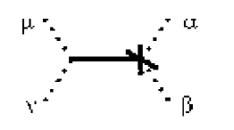
Figure 1: 4-tensor $\partial_{\mu}\partial_{\nu}h_{\alpha\beta}$

Dotted lines, a rigid line, a vertex with and without a crossing mark are called suffix-lines, a bond, a h-vertex and a dd-vertex respectively. We graphically represent suffix contraction by gluing two corresponding suffix-lines. As an example, $A1=\partial_{\sigma}\partial_{\lambda}h_{\mu\nu}\cdot\partial_{\sigma}\partial_{\nu}h_{\mu\lambda}$ is represented in Fig.2.

Figure 2: Graphical representation of $A1=\partial_{\sigma}\partial_{\lambda}h_{\mu\nu}\cdot\partial_{\sigma}\partial_{\nu}h_{\mu\lambda}$.

Generally suffix-lines in a SO(n)-invariant are closed. We call these suffix-loops. Let us state a useful lemma on a general SO(n)-invariant made of $s$ $\partial\partial h$-tensors. It will be used in Sec.III to classify graphs in terms of the vertex (h or dd)-distribution in suffix-loops. .

Lemma

Let a general $(\partial\partial h)^{s}$-invariant ($s=1,2,\cdots$) have $\underline{l}$ suffix-loops. Let each loop have $v_{i}$ h-vertices and $w_{i}$ dd-vertices ($i=1,2,\cdots,\underline{l}-1,\underline{l}$). We have the following necessary conditions for $s,\underline{l},v_{i}\ \mbox{and }w_{i}$.

$$\sum_{i=1}^{\underline{l}}v_{i}=s{\quad,}\quad\sum_{i=1}^{\underline{l}}w_{i}=s{\quad,}$$

$$v_{i}\geq 0{\quad,}\quad w_{i}\geq 0{\quad,}\quad v_{i}+w_{i}\geq 1{\quad,}$$ (2)

$$v_{i}\ ,\ w_{i}\ =0,1,2,\cdots\quad,\quad\underline{l}=1,2,3,\cdots,2s-1,2s{\quad.}$$

It is useful, for classifying graphs, to introduce a bondless diagram which is obtained by deleting all bonds within a graph. For $A1$ of Fig.2, the corresponding bondless diagram is shown in Fig.3

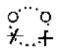
Figure 3: Bondless diagram for $A1$ of Fig.2. dd-vertices are explicitly represented by small circles.

, where a small circle is used to represent a dd-vertex explicitly.

Generally an SO(n)-invariant is composed of some suffix-loops. For each loop, we define two indices, the bond changing number (bcn) and the vertex changing number (vcn), in the following way.

Def

bcn[ ] and vcn[ ] are defined for each suffix-loop as follows[foot3]. When we trace the suffix-line of a suffix-loop, starting from a vertex in a certain direction, we generally pass some vertices, and finally come back to the starting vertex. When we move, in the tracing, from one vertex to the next vertex, we compare the bonds to which the two vertices belong, and their vertex types. If the bonds are different, we set $\Delta\mbox{\text@underline{bcn}}=1$, otherwise $\Delta\mbox{\text@underline{bcn}}=0$, If the vertex-types are different, we set $\Delta\mbox{\text@underline{vcn}}=1$, otherwise $\Delta\mbox{\text@underline{vcn}}=0$. For the i-th loop, we sum the number $\Delta\mbox{\text@underline{bcn}}$ and $\Delta\mbox{\text@underline{vcn}}$ while tracing the loop and assign as $\sum_{\mbox{along i-loop}}\Delta\mbox{\text@underline{bcn}}\equiv$ bcn[i], $\sum_{\mbox{along i-loop}}\Delta\mbox{\text@underline{vcn}}\equiv$ vcn[i].

bcn[ ] and vcn[ ] will be used, in Sec.IV and Sec.III respectively, for classifying graphs.

In paper (I), we have shown, using the graphical representation, that all independent invariants are

$$P\equiv\partial_{\mu}\partial_{\mu}h_{\alpha\alpha}{\quad,}\quad Q\equiv\partial_{\alpha}\partial_{\beta}h_{{\alpha\beta}}{\quad,}\quad$$ (3)

for $\partial\partial h$-invariants and

$$A1=\partial_{\sigma}\partial_{\lambda}h_{\mu\nu}\cdot\partial_{\sigma}\partial_{\nu}h_{\mu\lambda}\ ,\ A2=\partial_{\sigma}\partial_{\lambda}h_{\lambda\mu}\cdot\partial_{\sigma}\partial_{\nu}h_{{\mu\nu}}\ ,\ A3=\partial_{\sigma}\partial_{\lambda}h_{\lambda\mu}\cdot\partial_{\mu}\partial_{\nu}h_{\nu\sigma}\ ,$$

$$B1=\partial_{\nu}\partial_{\lambda}h_{\sigma\sigma}\cdot\partial_{\lambda}\partial_{\mu}h_{{\mu\nu}}\ ,\ B2=\partial^{2}h_{\lambda\nu}\cdot\partial_{\lambda}\partial_{\mu}h_{{\mu\nu}}\ ,\ B3=\partial_{\mu}\partial_{\nu}h_{\lambda\sigma}\cdot\partial_{\mu}\partial_{\nu}h_{{\lambda\sigma}}\ ,$$

$$B4=\partial_{\mu}\partial_{\nu}h_{\lambda\sigma}\cdot\partial_{\lambda}\partial_{\sigma}h_{{\mu\nu}}\ ,\ Q^{2}=(\partial_{\mu}\partial_{\nu}h_{{\mu\nu}})^{2}\ ,$$

$$C1=\partial_{\mu}\partial_{\nu}h_{\lambda\lambda}\cdot\partial_{\mu}\partial_{\nu}h_{\sigma\sigma}\ ,\ C2=\partial^{2}h_{{\mu\nu}}\cdot\partial^{2}h_{{\mu\nu}}\ ,\ C3=\partial_{\mu}\partial_{\nu}h_{\lambda\lambda}\cdot\partial^{2}h_{{\mu\nu}}\ ,$$

$$PQ=\partial^{2}h_{\lambda\lambda}\cdot\partial_{\mu}\partial_{\nu}h_{{\mu\nu}}\ ,\ P^{2}=(\partial^{2}h_{\lambda\lambda})^{2}\ ,$$ (4)

for $(\partial\partial h)^{2}$-invariants (totally 13 invariants). In Fig.4, an invariant $PQ$ in (4) is graphically shown.

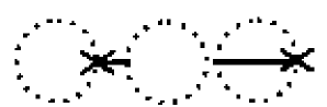
Figure 4: Graphical representation of $PQ=\partial^{2}h_{\lambda\lambda}\cdot\partial_{\mu}\partial_{\nu}h_{{\mu\nu}}$.

When a diagram is composed of some parts which are not connected by suffix-lines or bonds , as in Fig.4, we say it is disconnected. Otherwise , as in Fig.2, it is referred to as connected.

III Classification of $(\partial\partial h)^{3}$-Invariants by Bondless Diagrams

Let us first denote a suffix loop, with $v$ h-vertices, $w$ dd-vertices and a vertex changing number vcn as

$$\left(\begin{array}[]{c}v\\ w\end{array}\right)_{\mbox{\text@underline{vcn}}}{\quad.}$$ (7)

In Fig.5, all bondless diagrams that appear in suffix-loops of $(\partial\partial h)^{3}$-invariants, are displayed graphically with the above notation.

$\left(\begin{array}[]{c}3\\ 3\end{array}\right)_{6}$:  $\left(\begin{array}[]{c}3\\ 3\end{array}\right)_{4}$:  $\left(\begin{array}[]{c}3\\ 3\end{array}\right)_{2}$: 

$\left(\begin{array}[]{c}3\\ 2\end{array}\right)_{4}$:  $\left(\begin{array}[]{c}3\\ 2\end{array}\right)_{2}$:  $\left(\begin{array}[]{c}2\\ 3\end{array}\right)_{4}$:  $\left(\begin{array}[]{c}2\\ 3\end{array}\right)_{2}$: 

$\left(\begin{array}[]{c}2\\ 2\end{array}\right)_{4}$:  $\left(\begin{array}[]{c}2\\ 2\end{array}\right)_{2}$:  $\left(\begin{array}[]{c}3\\ 1\end{array}\right)_{2}$:  $\left(\begin{array}[]{c}1\\ 3\end{array}\right)_{2}$: 

$\left(\begin{array}[]{c}3\\ 0\end{array}\right)_{0}$:  $\left(\begin{array}[]{c}2\\ 1\end{array}\right)_{2}$:  $\left(\begin{array}[]{c}1\\ 2\end{array}\right)_{2}$:  $\left(\begin{array}[]{c}0\\ 3\end{array}\right)_{0}$: 

$\left(\begin{array}[]{c}2\\ 0\end{array}\right)_{0}$:  $\left(\begin{array}[]{c}1\\ 1\end{array}\right)_{2}$:  $\left(\begin{array}[]{c}0\\ 2\end{array}\right)_{0}$: 

$\left(\begin{array}[]{c}1\\ 0\end{array}\right)_{0}$:  $\left(\begin{array}[]{c}0\\ 1\end{array}\right)_{0}$: 

Figure 5: Bondless diagrams and values of ($v$, $w$, vcn).

In this section, we classify $(\partial\partial h)^{3}$-invariants by bondless diagrams. Taking $s=3$ in (2), we list up all cases as follows. In the following, vcn is omitted when the omission does not cause ambiguity in specifying a bondless diagram.

(i) $\underline{l}=1$

$$(1A):\left(\begin{array}[]{c}3\\ 3\end{array}\right)_{6}{\quad,}\quad(1B):\left(\begin{array}[]{c}3\\ 3\end{array}\right)_{4}{\quad,}\quad(1C):\left(\begin{array}[]{c}3\\ 3\end{array}\right)_{2}{\quad.}$$ (14)