Finite Size Scaling and Running Coupling Constant in $CP^{N-1}$ models

Abstract

In this work I present a numerical study of the Finite Size Scaling (FSS) of a correlation length in the framework of the $CP^{N-1}$ model by means of the $1/N$ expansion. This study has been thought as propedeutical to the application of FSS to the measure on the lattice of a new coupling constant $f_{x}(1/R)$, defined in terms or rectangular Wilson Loops. I give also a perturbative expansion of $f_{x}(1/R)$ in powers of the corresponding coupling constant in the $\overline{MS}$ scheme together with some preliminary numerical results obtained from the Polyakov ratio and I point out the conceptual problems that limit this approach.

I Introduction

A very important goal of a non perturbative approach to an asymptotically free theory such as the lattice is the determination of $\Lambda_{\overline{MS}}$ in a physical mass unit; this requires a very precise measurement of the ’running coupling’ $\alpha_{\overline{MS}}\left(\mu\right)$ for very large $\mu$. In order to perform the measure by a Monte Carlo simulation on a lattice it is useful to work in the framework of a new renormalization scheme, with its own renormalized coupling constant expandable in powers of $\alpha_{\overline{MS}}\left(\mu\right)$. This can be done defining a renormalized coupling constant in terms of rectangular Wilson loops. It is possible then to use Finite Size Scaling techniques to reach very small distances without very large lattices [1].

In this work I want to test this program in the framework of an abelian gauge theory in two dimensions: the $CP^{N-1}$ model. The choice of this specific model is justified by the fact that it is a renormalizable gauge theory and, above all, it shows both the asymptotic freedom and a confining potential between a particle-antiparticle pair, just as QCD does. Furthermore, $CP^{N-1}$ is simpler than QCD, being an abelian gauge theory in two dimensions and having the possibility of an expansion in powers of $1/N$, that can be efficiently used to test the new renormalization scheme and the new approach to the problem of computing $\Lambda_{\overline{MS}}$.

This paper is organized as follows: in section II I introduce the $CP^{N-1}$ model both in the continuum and on the lattice. In section III I apply the FSS technique to the study of the correlation length, trying to measure the $\Lambda$-parameter in two different renormalization schemes. In section IV I adopt the definition of the running coupling given in [1], whose perturbative expansion in powers of $f_{\overline{MS}}(\mu)$ is obtained. In section V I give some analytical and numerical results for the new coupling constant, obtained by means of the Polyakov and Creutz Ratio. In section VI I conclude with some considerations about the strategy outlined in the present work and I try to single out the ulterior difficulties that come out when one wants to apply the same technique to the study of the Creutz Ratio.

II The $CP^{N-1}$ model

The $CP^{N-1}$ model is a generalization of the non linear $\sigma$-models. The bare lagrangian of the continuum theory is:

$$L\left[z\left(x\right),\partial_{\mu}z\left(x\right),\lambda_{\mu}\left(x\right)\right]=\frac{N}{2f}\overline{D_{\mu}z\left(x\right)}D^{\mu}z\left(x\right)$$ (1)

where $z$ is a complex $N$-vector constrained by the condition $\overline{z(x)}z(x)=1$ and the operator $D_{\mu}$ is defined as $\partial_{\mu}+i\lambda_{\mu}$ .

As it is suggested by the mass dimension of the coupling constant $f$, the theory is renormalizable and it shows dimensional trasmutation [2, 3, 4].

Furthermore, the theory is expandable in powers of $1/N$; in this framework it is possible to show that the massless particles of the ‘standard’ perturbation theory acquire mass at the leading order in $1/N$ and they interact by a linear confining potential [2, 3, 5].

A very good reference for the theory of spin models on the lattice is [6], where we find a convenient lattice action of the $CP^{N-1}$ model, the gap equation, the inverse propagators $\Delta^{-1}_{\alpha}$ and $\Delta^{-1}_{\theta}$ of the effective fields and the definition of a correlation length $\xi_{L}$ that I report here:

$$\xi_{L}^{2}=\frac{1}{4\sin{}^{2}\frac{\pi}{L}}\left[\frac{\widetilde{G}_{P}\left(0,0;L\right)}{\widetilde{G}_{P}\left(0,1;L\right)}-1\right]$$ (2)

Where $G_{P}$ is the two-point correlation function of gauge invariant operator and $\widetilde{G_{P}}$ is its Fourier Transform. We can write $\widetilde{G}_{P}(k_{1},k_{2};L)$ as a function of the propagator of the effective field $\alpha$ in the framework of the $1/N$ expansion on a finite lattice:

$$\widetilde{G}_{P}\left(k;L\right)=\frac{1}{\beta^{2}}\Delta_{\left(\alpha\right)}^{-1}\left(k;L\right)+O\left(\frac{1}{N}\right)$$ (3)

where $\Delta_{\left(\alpha\right)}^{-1}\left(k_{1},k_{2};L\right)$ is given in [6]. Using the gap equation on a finite lattice [6] I can write the function $\xi_{L}\left(\beta\right)$ in a parametric form (with $m_{L}$ used as a parameter):

$$\begin{array}[]{lcl}\xi_{L}^{2}\left(m_{L}\right)&=&\frac{1}{4\sin{}^{2}\frac{\pi}{L}}\left[\frac{\Delta_{\left(\alpha\right)}^{-1}\left(0,0;L;m_{L}\right)}{\Delta_{\left(\alpha\right)}^{-1}\left(0,1;L;m_{L}\right)}-1\right]\\ \beta\left(m_{L}\right)&=&\frac{1}{L^{2}}\sum_{p}\frac{1}{\widehat{p}^{2}+m_{L}^{2}}\end{array}$$ (4)

Let us consider now the infinite lattice limit of the correlation length so defined. Manipulating the formulae in [6], it is easy to show that $\xi_{\infty}(\beta)$ has the following asymptotic form:

$$\xi_{\infty}\left(\beta\right)\simeq\frac{1}{8\sqrt{3}}e^{2\pi\beta}$$ (5)

III Finite Size Scaling of the Correlation Length

A complete theory of the Finite Size Scaling is contained in [9, 10], while an explanation of the strategy used in what follows and the definition of the various FSS functions can be found in [11, 12]. The FSS says that:

$$\xi_{L}\left(\beta\right)\simeq f_{P}\left(\frac{L}{\xi_{L}\left(\beta\right)}\right)\xi_{\infty}\left(\beta\right)$$ (6)

or equivalently

$$\frac{\xi_{L_{2}}\left(\beta\right)}{\xi_{L_{1}}\left(\beta\right)}\simeq\sigma_{\xi}\left(\frac{L_{2}}{L_{1}},\frac{L_{1}}{\xi_{L_{1}}\left(\beta\right)}\right)$$ (7)

I have used the expressions reported in [6] in the framework of the $1/N$ expansion, instead of a standard Monte Carlo simulations, in order to evaluate numerically the correlation length. The numerical computations have been performed by means of a FORTRAN code, choosing lattices of sizes varying from $L=20$ to $L=2000$.

A Computation of $a\Lambda_{LAT}$

The results of these computations are showed on the figure 1.

FIG. 1.: Function $\xi_{L}(\beta)$ for some values of $L$.

From these data I can extract a measure of the $\Lambda$-parameter in the lattice regularization scheme, defined by the perturbative two-loop solution of the renormalization group equation for the coupling constant in the large $N$ limit as reported in (5)

$$\frac{\xi\left(\beta\right)}{a}=\frac{1}{a\Lambda_{LAT}}e^{2\pi\beta}$$ (8)

The difference between $a\Lambda_{LAT}$ extracted from the lattice and the theoretical value $8\sqrt{3}$ (cfr. (5)) is below $3.2\%$. An equivalent way to test the asymptotic scaling is to define an effective $\Lambda$-parameter :

$$\frac{1}{\Lambda_{eff}(\beta)}=\xi_{\infty}(\beta)e^{-2\pi\beta}$$ (9)

and to plot the function

$$\frac{\Lambda_{LAT}}{\Lambda_{eff}}-1$$

versus $\xi_{\infty}(\beta)$, as showed in the figure 2.

FIG. 2.: Asymptotic scaling test.

The deviation from the asymptotic behaviour (5) is less than $2.6\times 10^{-6}$ for $\xi_{\infty}>90$.

B Computation of $\sigma_{\xi}(2,z_{L})$

I have computed the function $\sigma_{\xi}\left(2,z_{L}\right)$ , according to the scheme outlined in [12] and the figure 3 shows that it has these two asymptotic behaviours:

$$\lim_{z_{L}\rightarrow\infty}\sigma_{\xi}\left(2,z_{L}\right)=1~{}~{}~{}~{}~{}\lim_{z_{L}\rightarrow 0}\sigma_{\xi}\left(2,z_{L}\right)=2$$ (10)

that reflect these simple physical considerations:

1. In the limit $z_{L}\rightarrow\infty$ the actual size $L$ of the box is not very important because the correlation length $\xi_{L}(\beta)$ of the interaction is very small, compared to L; we are very close to the infinite volume limit.

2. In the limit $z_{L}\rightarrow 0$, on the contrary, the correlation length $\xi_{L}(\beta)$ is much larger than $L$, that becomes the actual scale of the interaction: the observables are very sensible to what happens on the border of the box; that is, $\xi_{L}(\beta)$, having the same dimension as $L$, is directly proportional to it.

If the FSS is correct, the function (7) should depend only on the ratio $\frac{L}{\xi_{L}}$, and not on $\xi_{L}$ and $L$ separately. I can check if this is the case by verifying that the several curves obtained on the different pairs of lattices approximately superimpose. The results are showed on the figure 3.

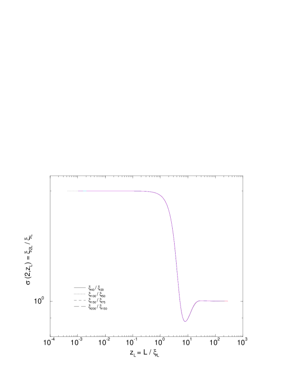
FIG. 3.: FSS function $\sigma_{\xi}(2,z_{L})$ for some values of $L$.

The biggest relative violation of the FSS is about $5.4\times 10^{-3}$ for $z_{L}=4.635...$

C Reconstruction of $f_{\xi}(z_{L})$

Now, in order to go on with the program outlined in [12], I need to know the function $\sigma_{\xi}\left(2,z_{L}\right)$ in every point of a sufficiently large interval; I have two possibilities:

1. interpolate the points I have obtained numerically using a polynomial of n-th degree, with n to be chosen.

2. find a suitable function that fits the points at our disposal very well. The theory [13] tells us that $\sigma_{\xi}(2,z_{L})\rightarrow 1$ exponentially fast as $z_{L}\rightarrow\infty$. Then I can try to use a fit function of the form

   $$\sigma_{\xi}^{(fit)}\left(2,z_{L}\right)=1+\sum_{n=1}^{N}a_{n}\exp\left(-nz_{L}/s\right)$$ (11)

   with the constraint that $\lim_{z_{L}\rightarrow 0}\sigma_{\xi}\left(2,z_{L}\right)=2$.

There are several systematic effects intrinsic in both procedures; I have made some checks in order to choose the values of the parameters that minimize them. Anyway, all ‘spurious’ systematic errors can be made smaller than the FSS violation, which in turn constitutes the real physical limit of our procedures. The figure 4 shows the results of the calculation.

FIG. 4.: FSS function $f_{\xi}(z_{L})$ computed in three different ways: a.Interpolation of $\sigma_{\xi}$. b.$15-$paramters fit of $\sigma_{\xi}$. c.Direct calculation of $f_{\xi}$ as $\frac{\xi_{L}}{\xi_{2000}}$.

D Perturbative expansion of $\sigma_{\xi}$ and $f_{\xi}$

A perturbative calculation on a finite lattice, along the line sketched in [14] gives the following result for the FSS function $f_{\xi}$:

$$f_{\xi}\left(z_{L}\right)=R\left(4\pi\right)^{2/N}e^{-d}z_{L}^{-1+4/N}e^{-4\pi/z_{L}^{2}}\left(1+O\left(z_{L}^{2}\right)\right)$$ (12)

with $R=\left(\xi_{\infty}\Lambda_{L}\right)^{-1}=8\sqrt{3}$ and $d=0.76077028681...$ In the large $N$ limit:

$$f_{\xi}\left(z_{L}\right)=Re^{-d}z_{L}^{-1}e^{-4\pi/z_{L}^{2}}\left(1+O\left(z_{L}^{2}\right)\right)$$ (13)

and

$$\sigma_{pert}\left(2,z_{L}\right)=2\left(1-\frac{\ln 2}{8\pi}z_{L}^{2}-\frac{\ln^{2}2}{64\pi^{2}}+O\left(z_{L}^{6}\right)\right)$$ (14)

I checked the range of validity of this perturbative result and I found good agreement for all $z_{L}<1$.

We can do this perturbative test on the function $f_{\xi}$ directly. If we look at the shape of the function $\sigma$_ξ we realize that the number of points in which it is necessary to know $\sigma_{\xi}$ itself in order to reconstruct $f_{\xi}$ is a decreasing function of $z_{L}$; this implies that a systematic error on the numerical computation of $\sigma$_ξ will propagate more and more when $z_{L}$ becomes smaller and smaller. This is exactly what I find if I compare the numerically reconstructed functions $f_{\xi}^{(fit)}$ and $f_{\xi}^{(int)}$ with the exact perturbative result (13). It is worth noticing that I can explain this effect quantitatively quite well invoking the FSS violation studied at the end of the paragraph III B.

E An asymptotic scaling test

It is worth noticing that in the large $N$ limit the FSS function $f_{\xi}(z_{L})$ is exactly known in terms of the two functions [15]:

$$F_{1}(z)=\frac{\pi}{z}-\log\pi+\frac{\log 2}{2}+\gamma_{E}+$$

$$+2\pi\sum_{n=1}^{\infty}\left(\frac{1}{\sqrt{4\pi^{2}n^{2}+z^{2}}}-\frac{1}{2\pi n}\right)+$$

$$+2\pi\sum_{n=-\infty}^{\infty}\frac{1}{\sqrt{4\pi^{2}n^{2}+z^{2}}}\frac{1}{\exp\left(\sqrt{4\pi^{2}n^{2}+z^{2}}\right)-1}$$ (15)

$$F_{2}(z)=\sum_{n=-\infty}^{\infty}\frac{1}{1-4n^{2}}\frac{\coth\left(\frac{\sqrt{4\pi^{2}n^{2}+z^{2}}}{2}\right)}{\sqrt{4\pi^{2}n^{2}+z^{2}}}$$ (16)

so we can obtain the function $f_{\xi}(z_{L})$ in a parametric form:

$$\begin{array}[]{lcl}f_{\xi}(x)&=&\frac{8\sqrt{3}}{z_{L}(x)}\exp\left[-F_{1}\left(\frac{1}{x}\right)\right]\\ z_{L}(x)&=&\frac{2\pi}{\sqrt{-1-\pi x\frac{F^{\prime}_{1}\left(\frac{1}{x}\right)}{F_{2}\left(\frac{1}{x}\right)}}}\end{array}$$ (17)

As already seen at the beginning of this section, the asymptotic behaviour of this expression is given by (13); in order to test the speed of approach to the asymptotic scaling I define from equation (13) the ‘asymptotic function’:

$$f_{\xi}^{as}(z_{L})=\Lambda_{FSS}\frac{e^{-\frac{4\pi}{z_{L}^{2}}}}{z_{L}}$$ (18)

where $\Lambda_{FSS}=Re^{-d}$ and $d=0.76077028681...$. I define also an effective $\Lambda_{FSS}$-parameter:

$$\Lambda_{FSS}^{eff}(z_{L})=f_{\xi}(z_{L})z_{L}e^{\frac{4\pi}{z_{L}^{2}}}$$ (19)

and I plot in the figure 5 the function

$$\frac{\Lambda_{FSS}^{eff}}{\Lambda_{FSS}}-1$$ (20)

that shows the deviation from the asymptotic scaling; this is less than $3.5\times 10^{-5}$ for $z_{L}<0.036$.

FIG. 5.: Asymptotic scaling test for the FSS function $f_{\xi}(z_{L})$

IV The ‘Running Coupling’ from Perturbation Theory

Following the procedure described in [1], let us consider a rectangular Wilson loop $(R\times T)$

$$W_{\Gamma}(R,T)=\left\langle e^{i\oint_{\Gamma}A_{\mu}(t)dt_{\mu}}\right\rangle$$ (21)

It is possible to give a definition of an interaction force $\chi_{T}(R)$ in which a partial derivative with respect to $T$ substitutes the $\lim_{T\rightarrow\infty}$ of the standard definition [16, 17]:

$$\chi(R,T)=\frac{\partial^{2}\ln W(R,T)}{\partial R\partial T}.$$ (22)

The perturbative expansion, in the continuum theory, of the interaction force $\chi_{T}(R)$ so defined is:

$$\chi^{\overline{MS}}_{T}(R)=\frac{N-1}{2\pi}I_{1}(x)\frac{t_{\overline{MS}}(\mu)^{2}}{R^{2}}\left\{1+2b_{0}\left[\ln(\mu R)+a(x)\right]t_{\overline{MS}}(\mu)+O(t_{\overline{MS}}(\mu)^{2})\right\}$$ (23)

where

$$I_{n}(x)=\int\frac{d^{2}q}{(2\pi)^{2}}q^{2}(\ln q)^{n}\frac{\sin q_{1}}{q_{1}}\frac{\sin(q_{0}x)}{q_{0}}$$ (24)

$$a(x)=1-\frac{I_{2}(x)}{2I_{1}(x)}$$ (25)

$x=\frac{T}{R}$, $t_{\overline{MS}}(\mu)$ is the renormalized coupling constant in the modified minimal subtraction scheme and $b_{0}$ is the first coefficient of the perturbative $\beta$ function of the model.

A direct computation of the integrals $I_{1}(x)$ and $I_{2}(x)$ gives:

$$I_{1}(x)=f(x)+\frac{1}{x^{2}}f\left(\frac{1}{x}\right)$$ (26)

with

$$f(x)=-\frac{1}{2\pi}\left(\arctan x+\frac{x}{1+x^{2}}\right)$$ (27)

and

$$I_{2}(x)=\frac{\gamma_{E}-1}{2}\left(1+\frac{1}{x^{2}}\right)-\frac{\ln x}{2x^{2}}-$$

$$-\frac{1}{\pi}\left\{B(x)+\frac{1}{x^{2}}\arctan x\ln x+\frac{1}{1+x^{2}}\left[\frac{\pi}{2}+\frac{1}{2}\ln(1+x^{2})\left(x+\frac{1}{x}\right)\right]+\right.$$

$$+\left.\int_{0}^{1}\frac{du}{u}\left[\frac{1}{x^{2}}\arctan\left(\frac{ux}{1+x^{2}(1-u)}\right)+\arctan\left(\frac{ux}{1+x^{2}-u}\right)\right]\right\}+$$

$$+\frac{x}{\pi}\int_{0}^{1}dt\,t^{2}\ln\left(\frac{1}{t^{2}}-1\right)\left[\frac{1}{(1+x^{2}t^{2})^{2}}+\frac{1}{(x^{2}+t^{2})^{2}}\right]$$ (28)

with

$$B(x)=g(x)+\frac{1}{x^{2}}g(\frac{1}{x})$$ (29)

and

$$g(x)=(\gamma_{E}-1)\arctan\frac{1}{x}-\gamma_{E}\frac{x}{1+x^{2}}-\arctan\frac{1}{x}\ln\frac{x}{1+x^{2}}$$ (30)

These functions have the following $x\rightarrow\infty$ limit:

$$\lim_{x\rightarrow\infty}I_{1}(x)=-\frac{1}{4}~{}~{}~{}~{}~{}\lim_{x\rightarrow\infty}I_{2}(x)=\frac{\gamma_{E}-1}{2}$$ (31)

Now it is possible to compute the function (25) numerically. The results are reported in the table I.

TABLE I.: Numerical value of the function $a(x)$ for some values of $x$.

$x$	$a(x)$	$x$	$a(x)$
$1$	$-0.289942...$	$4$	$-0.091605...$
$5/4$	$-0.450157...$	$5$	$0.007810...$
$4/3$	$-0.472398...$	$10$	$0.238997...$
$3/2$	$-0.488345...$	$50$	$0.478908...$
$5/3$	$-0.479687...$	$100$	$0.520289...$
$7/4$	$-0.469696...$	$200$	$0.544656...$
$2$	$-0.427594...$	$300$	$0.553868...$
$3$	$-0.234557...$	$\infty$	$0.577216...$

I can now define a running coupling constant $t_{x}(1/R)$:

$$\chi(R,T)=\frac{N-1}{2\pi}I_{1}(x)\frac{t_{x}(1/R)^{2}}{R^{2}}~{}~{}~{}~{}~{}~{}~{}~{}~{}x=\frac{T}{R}$$ (32)

and a large N-rescaled coupling constant $f_{x}(1/R)=Nt_{x}(1/R)/2$

$$\chi(R,T)=\frac{2}{\pi}\frac{N-1}{N^{2}}I_{1}(x)\frac{f_{x}(1/R)^{2}}{R^{2}}$$ (33)

The definition (32) and the perturbative result (23) allow to establish a link between $t_{x}\left(\frac{1}{R}\right)$ and $t_{\overline{MS}}\left(\mu\right)$:

$$t_{x}\left(\frac{1}{R}\right)^{2}=t_{\overline{MS}}\left(\mu\right)^{2}\left\{1+2b_{0}\left[a(x)+\ln\mu R\right]t_{\overline{MS}}\left(\mu\right)+O\left(t_{\overline{MS}}\left(\mu\right)^{2}\right)\right\}$$ (34)

where $a(x)$ determines the connection between the $\Lambda$-parameters in the two renormalization schemes:

$$a(x)=\ln\frac{\Lambda_{x}}{\Lambda_{\overline{MS}}}$$ (35)

V Analytical and Numerical results from the Polyakov Ratio

The Wilson line or Polyakov loop is strictly related to the static quark-antiquark potential [18]. I can take the interaction potential in the continuum theory for the case $x\rightarrow\infty$ from [5]:

$$V(R)=\frac{6\pi}{N}m_{0}^{2}R+\frac{2c_{L}}{N}m_{0}-\frac{2}{N}\int_{0}^{\infty}\cos(kR)\left[\Delta_{(\lambda)}(k)-\frac{12\pi m_{0}^{2}}{k^{2}}\right]\frac{dk}{2\pi}$$ (36)

where

$$\Delta_{(\lambda)}(k)=\frac{2\pi}{Y(k)\ln\frac{Y(k)+1}{Y(k)-1}-2}~{}~{}~{}Y(k)=\sqrt{1+\frac{4m_{0}^{2}}{k^{2}}}$$ (37)

After having rotated the integration contour in the complex plane and other algebraic manipulations I obtain

$$V(R)=\frac{6\pi}{N}m_{0}^{2}R+\frac{2c_{L}}{N}m_{0}+\frac{2\pi}{N}\int_{2m_{0}}^{\infty}e^{-xR}\frac{Y}{(\pi Y)^{2}+\left(Y\ln\frac{1+Y}{1-Y}-2\right)^{2}}$$ (38)

from which I can extract the interaction force

$$NF(R)\xi^{2}=\pi+\frac{\pi}{3}\int_{2}^{\infty}dte^{-\frac{tR}{\xi\sqrt{6}}}\frac{tY}{(\pi Y)^{2}+\left(Y\ln\frac{1+Y}{1-Y}-2\right)^{2}}=\Phi(r=\frac{R}{\xi})$$ (39)

where in (38) and (39) $Y(t)=\sqrt{1-\frac{4}{t^{2}}}$.

The formula (39) can be used to compute numerically the reference continuum quantity to be compared with the lattice results; it can also be expanded in the regime $r\rightarrow 0$ (perturbative or scaling region) obtaining the scaling behaviour of the interaction force:

$$\Phi(r)=\frac{\pi}{2}\frac{1}{r^{2}\ln^{2}\frac{\sqrt{6}}{r}}+\frac{\pi\gamma_{E}}{r^{2}\ln^{3}\frac{\sqrt{6}}{r}}+O(\frac{1}{r^{2}\ln^{4}\frac{\sqrt{6}}{r}})$$ (40)

This result can be rewritten with the same precision as

$$\Phi(r)=\frac{\pi}{2}\frac{1}{r^{2}\ln^{2}\frac{\sqrt{6}}{e^{\gamma_{E}}r}}\left(1+O(\frac{1}{r^{2}\ln^{4}\frac{\sqrt{6}}{r}})\right)$$ (41)

It is possible to extract from (41) the running coupling constant in the scheme outlined in the previous paragraph in the limit $x\rightarrow\infty$

$$f_{\infty}(r)=\frac{\pi}{\ln\frac{\sqrt{6}}{e^{\gamma_{E}}r}}$$ (42)

This expression is in perfect agreement with the prediction of the 1-loop perturbative renormalization group

$$\Phi(r)=\frac{\pi}{2}\frac{1}{r^{2}\ln^{2}\frac{1}{\Lambda_{\infty}R}}$$ (43)

if the $\Lambda$-parameter is chosen consistently with the renormalization scheme introduced before :

$$\Lambda_{\infty}R=e^{a(\infty)}\Lambda_{\overline{MS}}R=e^{\gamma_{E}}r/\sqrt{6}$$ (44)

The difference between the exact continuum curve and the asymptotic one is below $5\%$ for $r<0.25$. One could then measure the interaction force on a finite lattice by means of the so-called Polyakov Ratio, for several values of $r_{L}<0.25$, keeping $z_{L}$ fixed, and then fit the values with equation (43) in order to extract the $\Lambda$-parameter. It is so possible to understand how fast the measures on the lattice approach the continuum limit (44) when the lattice spacing goes to 0.

The Polyakov Ratio on a finite lattice with periodic boundary conditions is given by

$$\chi_{P}(R)=\frac{1}{L}\ln\frac{W(R,L)}{W(R-1,L)}=-\frac{1}{2N}\frac{1}{L}\sum_{k}\frac{\sin\frac{k_{1}(2R-1)\pi}{L}}{\sin\frac{k_{1}\pi}{L}}\widehat{k_{1}}^{2}\Delta_{(\theta)}(k_{1},0)$$ (45)

in the leading order in the $1/N$ expansion, where $\Delta_{(\theta)}(k)$ is the lattice propagator of the gauge field $\theta$ reported in [6].

FIG. 6.: Systematic effect $\propto a/R$ on the value of the Polyakov ratio on a finite lattices. The continuum line is the continuum interaction force 40

A numerical calculation of the Polyakov Ratio has been performed on two lattices ($L=1000$ and $L=2000$) and for two $\xi_{L}$, keeping $z_{L}=19.455...$ fixed. The results are showed on the figure 6, where we can see the presence of a systematic effect $\propto a/R$ for $r=R/\xi_{L}<0.25$; when $r>0.25$ other effects due to periodicity start to play a much more important role [6, 19].

VI Conclusions and Outlook

The study of the correlation length has clarified how to use the FSS technique to estrapolate the finite volume measures to infinite volume results. In this framework it could be interesting to apply the same technique to a basic observable: the Creutz Ratio derived from rectangular Wilson loops. Even if this seems to be just a mere step-by-step execution of the program already outlined in [12] for the correlation length, there are some points that should be underlined:

1. the presence of the additional scale $R$ implies that the FSS function depends on two variables, instead of only one.

2. a systematic effect $\propto\left(\frac{a}{R}\right)^{2}$ (analogous to that found in the case of the Polyakov Ratio) is present in the Wilson loop case, too.

3. in the special case of an abelian lattice gauge theory defined on a torus, as our version of the lattice $CP^{N-1}$ model is, there are some kinematical effects that have to be considered in order to obtain significant results [19].

4. the special shape of the FSS function $\sigma_{\xi}\left(2,z_{L}\right)$ imposes another limitation on the region where the FSS technique can be applied efficiently: let us define

   $$\Phi(\beta,R,x,L)=\chi(\beta,R,xR,L)$$ (46)

   $\Phi$ obeys to a FSS law similar to (6) seen in the section III for the correlation length:

   $$\Phi\left(x,\beta,R,L\right)=g_{\Phi}\left(x,\frac{R}{\xi_{L}(\beta)},\frac{L}{\xi_{L}(\beta)}\right)\Phi\left(x,\beta,R,\infty\right)$$ (47)

   The counterpart of the function $\sigma_{\xi}$ is

   $$s_{a,b}(z_{L},r_{L})=\lim_{\beta\rightarrow\infty}\frac{\Phi(\beta,bR,x,aL)}{\Phi(\beta,R,x,L)}$$ (48)

   where

   $$z_{L}=\frac{L}{\xi_{L}(\beta)}~{}~{}~{}r_{L}=\frac{R}{\xi_{L}(\beta)}$$ (49)

   The limit $\beta\rightarrow\infty$ means simply that we are in the scaling region. If the FSS law (47) is valid and choosing $a=2$, $b=1$

   $$s_{2,1}(z_{L},r_{L})=\frac{g_{\Phi}(x,z^{\prime}_{L},r^{\prime}_{L})}{g_{\Phi}(x,z_{L},r_{L})}=\frac{\Phi(\beta,R,x,2L)}{\Phi(\beta,R,x,L)}$$ (50)

   with

   $$z^{\prime}_{L}=\frac{2z_{L}}{\sigma_{\xi}\left(2,z_{L}\right)}~{}~{}~{}r^{\prime}_{L}=\frac{r_{L}}{\sigma_{\xi}\left(2,z_{L}\right)}$$ (51)

   Once I have measured the function $s_{2,1}(z_{L},r_{L})$ in a large enough region of the plane $(z_{L},r_{L})$, I can try to reconstruct the function $g_{\Phi}(x,z_{L},r_{L})$ by:

   $$g_{\Phi}(x,z_{L},r_{L})\simeq\prod_{j=1}^{n}\frac{1}{s_{2,1}(z^{(j)}_{L},r^{(j)}_{L})}g_{\Phi}(x,z^{(n)}_{L},r^{(n)}_{L})$$ (52)

   with

   $$z^{(j)}_{L}=\frac{2z^{(j-1)}_{L}}{\sigma\left(2,z^{(j-1)}_{L}\right)}~{}~{}~{}r^{(j)}_{L}=\frac{r^{(j-1)}_{L}}{\sigma\left(2,z^{(j-1)}_{L}\right)}$$ (53)

   A severe limitation to this computational scheme is represented by the practical impossibility to reach very small values of $L/\xi_{L}(\beta)$. From figure 3 we see that $\sigma_{\xi}\simeq 2$ for $L/\xi_{L}(\beta)<1$. When we try to compute $g_{\Phi}$ for a $L/\xi_{L}(\beta)$ quite small, $\sigma_{\xi}(2,z_{L}^{(j)})$ in (53) stays very close to $2$ even for $\overline{\j}$ very large; now, for $\j<\overline{\j}$, while $r_{L}$ is reduced to a half at each step, $z_{L}$ stays about constant (remember (51)). I can do two things, in order to lessen $r_{L}$: I can lessen $R$, and, once I have reached the lowest limit for $R$, since $a$ is finite, I must increase $\xi_{L}(\beta)$, and this means that I have to increase $L$ too, to keep $z_{L}$ constant. In conclusion, if I want to compute the function $g_{\Phi}(x,z_{L},r_{L})$ for a very small $z_{L}$ I need to simulate on very large lattices, or, in other words, a upper limit on the size $L$ of the lattice implies a lower limit on $z_{L}$, as far as the measure of $g_{\Phi}(x,z_{L},r_{L})$ concerns.

These considerations leads to the conclusion that the application of the FSS technique to the Wilson loop needs a careful study of all the systematic effects. Furthermore, the problem outlined in the last point above seems to limit the efficiency of the method in the region where also the traditional techniques fail. The crucial point is represented by the exact form of $\sigma_{\xi}(2,z_{L})$ when $z_{L}\rightarrow 0$. Once I have fixed the largest dimension $L_{MAX}$ of a usable lattice, the lowest limit $z_{L}^{(min)}$ at which it is possible to compute the function $g_{\Phi}(x,z_{L},r_{L})$ is different from $0$ and it depends on the specific definition of the correlation length chosen. The only thing we can do is to find a correlation length that minimizes $z_{L}^{(min)}$.

VII Aknowledgements

I would like to thank P. ROSSI, E. VICARI and A. PELISSETTO for their useful comments and suggestions.

REFERENCES

- [1] M.Campostrini, P.Rossi, E.Vicari, Phys. Lett. 349B, 499 (1995)
- [2] H.Eichenherr, Nucl. Phys. B146, 223 (1978)
- [3] A.D’Adda, M.Luscher, P.Di Vecchia, Nucl. Phys. b146, 63(1978)
- [4] G.Valent, Nucl. Phys. B238, 142 (1984)
- [5] M.Campostrini, P.Rossi, Phys. Rev. D45, 618,(1992) ; D46, 2741 (1992) (E)
- [6] M.Campostrini, P.Rossi, Rivista del Nuovo Cimento, Vol. 16-I, serie 3, n. 6 (1993)
- [7] M.Campostrini, P.Rossi, E.Vicari, Phys. Rev. D46, 4643 (1992)
- [8] M.Campostrini, P.Rossi, E.Vicari, Phys. Rev. D46, 2647 (1992)
- [9] E.Brézin, J.Physique, 43, 15 (1982)
- [10] J.L.Cardy, ed., Finite-size scaling (North-Holland, Amsterdam, 1988)
- [11] M.Lüscher, P.Weisz, U.Wolff, Nucl. Phys. B359, 221, (1991); M.Lüscher, R.Sommer, U.Wolff, P.Weisz, Nucl. Phys. B389, 247, (1993)
- [12] S.Caracciolo, R.G.Edwards, S.J.Ferreira, A.Pelissetto, A.D.Sokal, Nucl. Phys. B (Proc. Suppl.), 42, 749 (1995)
- [13] H.Neuberger, Phys. Lett. B233, 183 (1989)
- [14] P.Hasenfratz, Phys. Lett. 141B, 385 (1984)
- [15] A.Pelissetto, private communication
- [16] L.S.Brown, W.I.Weisberger, Phys.Rev. D20, 3239 (1979)
- [17] K.Wilson, Phys.Rev. D10, 2445 (1974)
- [18] H.J.Rothe, Lattice Gauge Theories : An Introduction, World Scientific
- [19] P.Rossi, E.Vicari, Phys. Rev. D48, 3869, (1993)