Abstract

A basis of Lorentz and gauge-invariant monomials in non-Abelian gauge theories with matter is described, applicable for the inverse mass expansion of effective actions. An algorithm to convert a arbitrarily given invariant expression into a linear combination of the basis elements is presented. The linear independence of the basis invariants is proven.

1 Introduction

One-loop effective actions [1] are space-time integrals of Lorentz and gauge-invariant expressions. They are closely related to traces of heat kernels, known as Schwinger-DeWitt [2], Gilkey-Seeley [3], or Hadamard [4] coefficients. In flat space-time gauge theory, these coefficients are polynomials consisting of a matrix potential, the gauge-field strength tensor, and gauge-covariant derivatives. There are many equivalent forms for these coefficients essentially due to the Bianchi identity and the product rule for covariant derivatives. Furthermore, the physically interesting functional trace allows one to cyclically exchange matrix factors and to integrate by parts.

Increasing use of computer algebra [5] and new methods to calculate effective actions [6, 7] extend our knowledge of heat kernel coefficients to higher and higher order. To manage the increasing number of terms in them and compare results obtained by different methods, a minimal set of invariants is needed in terms of which all results can be expressed. In addition, an algorithm to expand a given gauge-invariant Lorentz scalar into this minimal set should be provided.

This problem was mainly considered in general relativity where the tensor polynomials consist of the Riemann tensor, the metric tensor, and covariant derivatives. This is more complicated than flat space-time gauge theory due to the symmetry properties of the Riemann tensor. However, Fulling et al. [8] used group representation methods to determine the numbers of independent monomials, so that an appropriate subset of all monomials can be chosen to be a basis. Nevertheless, this subset has to be chosen by hand because there is no known general construction principle.

For gauge theory in flat space-time, van de Ven [9] constructed a basis up to mass dimension ten (fifth order of the inverse mass expansion). But he also chose the basis elements by hand and did not present a general construction principle.

For the expansion of effective actions of matter, gauge fields, and gravity in terms of Barvinsky-Vilkovisky form factors [10], a basis set of non-local invariants up to third order in the curvature was defined [11].

The present article, extending our work in Ref. [12], analyses the formal structure of Lorentz and gauge-invariant monomials in non-Abelian gauge theories with matter in flat space-time. Step by step, the operations applicable to these invariants are used to bring them into a form consisting of special invariant monomials. These are proven to be linearly independent. Thus, a basis set of invariants is specified, and simultaneously, a procedure to expand a given Lorentz and gauge-invariant expression in terms of the basis is obtained.

Section 2 introduces notations, manipulations applicable to invariants, and a graphical representation of invariants, which is needed for the proof of linear independence. Section 3 describes the algorithm to expand a given gauge-invariant Lorentz scalar in terms of special gauge-invariant monomials. The properties of these monomials are summarized in Section 4. They are used to count the special monomials up to mass dimension 16. Section 5 shows that this set of monomials is linearly independent and therefore a basis. We summarize in Section 6. Appendix A describes manipulations with fully symmetrized covariant derivatives. The numbers of independent invariants, subdivided by the number of matrix potentials and field-strength tensors, are given in Appendix B. Also the basis invariants up to mass dimension eight are listed there explicitly. Appendix C describes a construction needed for the proof of linear independence.

2 Notations and representation by graphs

We consider a gauged scalar field theory described by the massive complex field $\phi^{a}$ and the hermitian matrix valued gauge field $A_{\mu}^{ab}$. The gauge-covariant derivative in the fundamental representation is ${\cal D}_{\mu}^{ab}=\delta^{ab}\partial_{\mu}-{\rm i}A_{\mu}^{ab}$. The coupling constant is absorbed into the gauge field. The matter field contribution to the effective one-loop action is given by

$$\Gamma^{(1)}[\varphi,A]={\rm\;Tr}\ln\left(-{\cal D}^{2}+m^{2}+V\right)=-\int_{0}^{\infty}\frac{{\rm d}T}{T}{\rm e}^{-Tm^{2}}{\rm\;Tr}\exp\left(-T\left(-{\cal D}^{2}+V\right)\right)$$ (1)

The integral in Equation (1) is to be understood regularized at $T=0$ in some way, e.g. by dimensional regularization [13], by the zeta function procedure [14] or by a cut-off. The trace of the heat kernel can be evaluated by various methods [6, 7, 15] and expanded in gauge-invariant terms [5, 6, 7, 9, 15, 16]

$${\rm\;Tr}\exp\left(-T\left(-{\cal D}^{2}+V\right)\right)=\int{\rm d}^{d}x{\rm\;tr}\sum_{i}C_{i}{T^{\frac{\mu_{i}-d}{2}}}I_{i}\left(F,V\right).$$ (2)

The matrix potential $V$ is hermitian and originates from the self-interaction of the matter field. $C_{i}$ are in general complex dimensionless numbers. The space-time dimension is defined to be $d$. $I_{i}\left(F,V\right)$ are matrix valued Lorentz scalars which are composed of the matrix potential $V$, the field strength tensor

$$F_{\mu\nu}^{ab}={\rm i}\left[{\cal D}_{\mu},{\cal D}_{\nu}\right]^{ab}=\partial_{\mu}A_{\nu}^{ab}-\partial_{\nu}A_{\mu}^{ab}-{\rm i}\left[A_{\mu},A_{\nu}\right]^{ab},$$ (3)

and the adjoint gauge-covariant derivative

$$D_{\mu}=\left[{\cal D}_{\mu},\,\right]=\partial_{\mu}-{\rm i}\left[A_{\mu},\,\right].$$ (4)

$D_{\mu}$ acts on $V$ and on $F_{\mu\nu}$. $\mu_{i}$ is the mass dimension of the Lorentz scalar $I_{i}\left(F,V\right)$ according to the mass dimensions of its constituents $[V]=2$, $[F_{\mu\nu}]=2$, and $[D_{\mu}]=[{\cal D}_{\mu}]=1$. The first few terms of the expansion (2) are [16]

$${\rm\;Tr}\exp\left(-T\left(-{\cal D}^{2}+V\right)\right)=\left(4\pi T\right)^{-\frac{d}{2}}\int{\rm d}^{d}x{\rm\;tr}\left[{\rm 1\!\!\!\;l}-TV+\frac{T^{2}}{2}\left(V^{2}+\frac{1}{6}F_{\mu\nu}F_{\mu\nu}\right)+\ldots\right].$$ (5)

The form (2) is not unique due to the possible manipulations of Table 1. In this article, we call the possibility of cyclic matrix permutations under the trace cyclic invariance, and that of mirror transformations reflection invariance. The latter stems from the possibility of matrix transpositions under the trace. The scope of the present article is to fix all manipulation possibilities and to obtain a basis for the gauge-invariant Lorentz scalars $I_{i}(F,V)$.

Table 1: The possible manipulations applicable to Lorentz scalars $I_{i}(F,V)$ and the corresponding equalities that are used. Integration by parts assumes the background fields decrease sufficiently quickly at infinity. In the last line, $X$, $Y$, and $Z$ are assumed to be “simple factors” (defined in the text). Further relations between invariants such as equations of motion or additional symmetries are not taken into account.

Manipulation	Used equality
Product rule	$D_{\mu}(XY)=D_{\mu}XY+XD_{\mu}Y$
Cyclic matrix permutations	${\rm\;tr}(XYZ)={\rm\;tr}(YZX)$
Integration by parts	$\int{\rm d}x{\rm\;tr}\left(D_{\mu}X_{\mu}Y\right)=-\int{\rm d}x{\rm\;tr}\left(X_{\mu}D_{\mu}Y\right)$
Bianchi identity	$D_{\mu}F_{\kappa\lambda}=D_{\kappa}F_{\mu\lambda}+D_{\lambda}F_{\kappa\mu}$
Antisymmetry of $F_{\mu\nu}$	$F_{\mu\nu}=-F_{\nu\mu}$
Mirror transformation	$\overline{{\rm\;tr}\left(XYZ\ldots\right)}={\rm\;tr}\left(\ldots Z^{\dagger}Y^{\dagger}X^{\dagger}\right)={\rm\;tr}\left(\ldots ZYX\right)$

We introduce some further terminology. $V$, $F_{\kappa\lambda}$, $D_{\mu_{1}}D_{\mu_{2}}\ldots D_{\mu_{n}}V$, or $D_{\mu_{1}}D_{\mu_{2}}\ldots D_{\mu_{n}}F_{\kappa\lambda}$ ($n\geq 1$) are simple factors. Containing $V$ they are called $V$-factors, otherwise $F$-factors. Simple invariants or invariant monomials are products of simple factors.

Due to the hermiticity of $A_{\mu}$ simple factors are always hermitian

$$V^{\dagger}=V,\quad\quad F_{\mu\nu}^{\dagger}=F_{\mu\nu},\quad\quad X^{\dagger}=X\quad\Longrightarrow\quad\left(D_{\mu}X\right)^{\dagger}=D_{\mu}X.$$ (6)

This property provides the basis for the reflection invariance of simple invariants.

Applying the product rule for covariant derivatives, the invariants $I_{i}(F,V)$ of Equation (2) may always be expressed by sums of simple invariants. Therefore we assume in the following all invariants $I_{i}(F,V)$ to be simple.

The last manipulation of Table 1 is called mirror transformation because it inverts the ordering of the factors $X$, $Y$, and $Z$. It relates an invariant with the complex conjugate of another one. Generically, a quantity and its complex conjugate are linearly independent, and the mirror transformation cannot be used to substitute an invariant by another one. But in special situations this transformation is useful. Assuming the effective action (2) is real, then — expanded in an appropriate basis — every simple invariant $I_{1}={\rm\;tr}\left(XYZ\ldots\right)$ and its mirror image $I_{2}={\rm\;tr}\left(ZYX\ldots\right)=\overline{I_{1}}$ have coefficients $C_{1}$ and $C_{2}$ complex conjugate to each other, so that the sum of them can be written as $C_{1}I_{1}+C_{2}I_{2}=2\Re{\rm e}\left(C_{1}I_{1}\right)$. Obviously $I_{2}$ was replaced by $I_{1}$ but the price paid is the introduction of the projection operator $\Re{\rm e}$. Another special situation is a real field $\phi^{a}$ and a real representation of the gauge group. $V$ is then real and symmetric, whereas $A_{\mu}$ and $F_{\mu\nu}$ are imaginary and antisymmetric (thus still hermitian). The simple invariants and its complex conjugates are then equal up to a factor of $(-1)^{f}$ (where $f$ is the number of $F$-factors in the corresponding invariant).

The ordering of derivatives within a factor can be changed by continued application of

$$D_{\mu}D_{\nu}X=D_{\nu}D_{\mu}X-{\rm i}\left[F_{\mu\nu},X\right].$$ (7)

This produces additional terms with more $F$-factors and fewer derivatives. After the commutation of some inner derivatives the product rule has to be applied again. In this way every ordering of derivatives can be achieved.

The indices in a simple invariant can be contracted between different factors and within the same factor. Let us consider the latter case, we call it self-contraction. At least one index must belong to a derivative, otherwise it would be the contraction $F_{\mu\mu}$ which forces the whole invariant to vanish. After commuting this derivative to the outside of the factor, integration by parts can be applied. In the resulting expression one self-contraction has been eliminated. Repeating this, we arrive at an expression where all invariants $I_{i}(F,V)$ have no self-contractions. From now on we assume our gauge- and Lorentz-invariant expression (2) to have this form.

Now we are able to introduce the graphical representation of simple invariants. The factors are represented by regions located on a circle (cf. Tab. 2 and Fig. 1). The circle takes into account the cyclic invariance of the trace. Reading the invariant from left to right corresponds to reading the graph counterclockwise along the circle.

Table 2: Graphical elements for the representation of simple invariants

Part of a term	Graphical representation
$V$	$\bullet$
$F_{\mu\nu}$
$D_{\mu}$	$\circ-\!\!\!--\!\!\!-\!\!\!-\mu$

(a)    (b)    (c)    (d)   

Figure 1: Examples for the graphical representation of terms: (a) ${\rm\;tr}(F_{\mu\nu}F_{\mu\nu})$, (b) ${\rm\;tr}(F_{\mu\nu}D_{\mu}VD_{\nu}V)$, (c) ${\rm\;tr}(F_{\mu\nu}F_{\kappa\mu}F_{\nu\kappa})$, (d) ${\rm\;tr}(F_{\mu\nu}F_{\kappa\mu}D_{\nu}F_{\lambda\kappa}D_{\lambda}V)$.

Contractions between factors are represented by straight lines connecting the regions. Open points at the line ends symbolize derivatives. $V$’s are depicted by closed points. $F_{\mu\nu}$’s are recognizable by two linked lines representing the two indices. The representation of simple invariants by graphs is unambiguous only modulo permutations of derivatives (7) and index interchanges in $F_{\mu\nu}$’s. This ambiguity can be eliminated by choosing a certain index ordering for the invariants. This will be done below where the algorithm for expanding a given invariant in basis invariants is described.

3 The algorithm

This section describes an algorithm using the manipulations of Table 1 to transform an arbitrary expression (2) into a standard form. Section 5 will show that the invariant monomials left unchanged by the algorithm are linearly independent, at least if we exclude mirror transformations from the possible manipulations of Table 1 (including mirror transformations the same is true at least up to 16 mass dimensions, as we will see below). Therefore the result of the algorithm, expressed by the basis invariants, will always be unique, though the algorithm may offer at intermediate stages several possibilities to proceed.

We start with an arbitrary Lorentz and gauge-invariant expression of the form (2). We treat invariants with different mass dimension separately, since the manipulations of Table 1 do not mix them. In Section 2 the product rule and integration by parts were used to obtain a sum of simple invariants which have no self-contractions and can be represented by graphs. This is the first step of the algorithm.

The following steps require commutations of derivatives by Equation (7), which produce additional invariant monomials containing more $F$-factors and fewer derivatives. Therefore we concentrate on the invariant monomials not in their final form and having the fewest $F$-factors (or alternatively, the most derivatives, i.e. the fewest factors). Then the following steps of the algorithm are applied to these monomials, transforming them into their final form and falling out of the consideration. This procedure is iterated until all monomials are in their final form.

The first step inside the iteration is to use the Bianchi identity. This identity interchanges the index of a derivative with the indices of the field strength tensor within an $F$-factor, without disturbing the other factors. To apply the Bianchi identity to an $F$-factor with more than one derivatives we must specify the derivative which we want to use and commute it with the other derivatives by Equation (7) so that it becomes the innermost derivative. Which derivatives do we specify? We look at the example

$${\rm\;tr}(\underbrace{\stackrel{{\scriptstyle\mbox{L}}}{{D_{\mu}}}\stackrel{{\scriptstyle\mbox{R}}}{{D_{\nu}}}\stackrel{{\scriptstyle\mbox{M}}}{{D_{\rho}}}D_{\sigma}F_{\kappa\lambda}}_{\makebox[0.0pt]{\parbox{71.13188pt}{\centering factor under\\ consideration\@add@centering}}}\underbrace{\ldots X_{\nu}^{\prime}\ldots}_{\parbox{42.67912pt}{\centering right sector\@add@centering}}Y_{\sigma\kappa}\underbrace{\ldots X_{\rho}^{\prime\prime}\ldots}_{\parbox{42.67912pt}{\centering middle sector\@add@centering}}Z_{\lambda}\underbrace{\rule{0.0pt}{7.96527pt}\ldots X_{\mu}\ldots}_{\makebox[0.0pt][l]{\parbox{42.67912pt}{\centering left sector\@add@centering}}})\quad.$$ (8)

The indices of $F_{\kappa\lambda}$ are contracted with the factors $Y_{\sigma\kappa}$ and $Z_{\lambda}$, which divide the remaining factors into three, possibly empty, sectors. These are denoted by “right sector”, “middle sector”, and “left sector”, because the “left sector” is connected with the left-hand side of the considered factor by cyclic invariance. This is depicted in Figure 2.

        L               M                       R

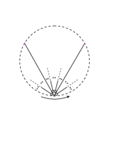
Figure 2: A certain $F$-factor within a graph. The two $F$-indices give rise to three sectors, marked with L, M, and R, with which the derivatives are contracted. Following the arrow corresponds to reading the invariant monomial from the left to the right.

The derivatives of the factor under consideration are called left (“L”), right (“R”), and middle (“M”) corresponding to the sector with which they are contracted. Not all derivatives are left, right, or middle (e.g. $D_{\sigma}$). The Bianchi identity mixes all three kinds of derivatives. Therefore it can be used to eliminate one kind of derivative in all factors of all monomials. Since the middle sector is invariant under the mirror transformation (left and right sectors are interchanged), we apply the Bianchi identity to middle derivatives. Each such application of the Bianchi identity reduces the number of factors in the corresponding middle sector. So after a finite number of steps, all middle derivatives are eliminated.

Next, we convert multiple contractions between factors into a standard form by

$$\ldots F_{\mu\nu}\ldots D_{\mu}D_{\nu}X\ldots \Rightarrow -\frac{{\rm i}}{2}\ldots F_{\mu\nu}\ldots\left[F_{\mu\nu},X\right]\ldots$$ (9)

$$\ldots F_{\mu\nu}\ldots D_{\mu}F_{\nu\kappa}\ldots \Rightarrow \frac{1}{2}\ldots F_{\mu\nu}\ldots D_{\kappa}F_{\nu\mu}\ldots$$ (10)

$$\ldots D_{\mu}F_{\nu\kappa}\ldots D_{\nu}F_{\mu\lambda}\ldots \Rightarrow \ldots D_{\mu}F_{\nu\kappa}\ldots D_{\mu}F_{\nu\lambda}\ldots+$$ (11)

$$\hskip 28.45274pt+\frac{1}{2}\ldots D_{\kappa}F_{\nu\mu}\ldots D_{\lambda}F_{\mu\nu}\ldots.$$

The first transformation uses the antisymmetry of the field strength tensor and the commutation rule (7). The second transformation relies again on the antisymmetry together with the Bianchi identity. The third equality results from the Bianchi identity for one of the factors and the second transformation (10).

The graphical representation of monomials automatically takes into account the cyclic invariance if we regard a certain graph and the same graph but rotated as identical. The reflection invariance can be taken into account by identification of graphs with their mirror images. In the analytic expressions we pick a representative of each class of equivalent “rotated” and “reflected” monomials, for instance the first or last monomial according to some lexicographical order.

The last step inside the above mentioned iteration is to arrange the derivatives and the indices of the field strength tensor in a definite way. This will be done factor by factor, such as for the application of the Bianchi identity. Here three prescriptions are proposed.

1) We consider a certain factor of a simple invariant. Temporarily suspending the fixing of the cyclic invariance, the factor is shifted to the left end of this monomial, as in example (8). We call two indices which are contracted with each other partners for the moment. We then rearrange the derivatives and indices of the field strength tensor (if present) in the considered factor so that they copy the ordering of their partner indices. In example (8) $Y_{\sigma\kappa}$ is located left of $Z_{\lambda}$, therefore the indices of $F_{\kappa\lambda}$ have the correct order. The locations of $X_{\nu}^{\prime}$, $Y_{\sigma\kappa}$, $X_{\rho}^{\prime\prime}$, and $X_{\mu}$ define the correct order of the derivatives to be $D_{\nu}D_{\sigma}D_{\rho}D_{\mu}$. While this arrangement of indices is independent of the fixing of the cyclic invariance due to the temporary shift, it is still dependent on mirror transformations, which invert the ordering of the factors. If we choose a different fixing of the reflection invariance we obtain a slightly different basis which results in different coefficients in front of the basis invariants. Since there appears to be no natural way to fix the reflection invariance, this prescription for the ordering of the indices seems to be sensible only if the problem we want to describe does not allow mirror transformations.

2) The second prescription is relatively simple and has no problems with the reflection invariance. The derivatives are symmetrized by forming the sum over all index permutations:

$$D_{\alpha_{1}\cdots\alpha_{k}}X\to D_{(\alpha_{1}\cdots\alpha_{k})}X=\frac{1}{k!}\sum_{\pi\in S_{k}}D_{\alpha_{\pi(1)}\cdots\alpha_{\pi(k)}}X.$$ (12)

This can be realized by successive application of

$$D_{\mu}D_{(\alpha_{1}\cdots\alpha_{k})}X=D_{(\mu\alpha_{1}\cdots\alpha_{k})}X-\frac{{\rm i}}{k+1}\sum_{\lambda=1}^{k}\left(\begin{array}[]{c}k+1\\ \lambda+1\end{array}\right)\left[D_{(\alpha_{1}\cdots\alpha_{\lambda-1}|}F_{\mu|\alpha_{\lambda}},D_{\alpha_{\lambda+1}\cdots\alpha_{k})}X\right].$$ (13)

This equation is derived in Appendix A. The indices of the field strength tensor are ordered as in the first prescription or somehow different — this is not so important because it produces only factors of $(\pm 1)$ and different conventions of this point can easily be converted. Working with this prescription, it is more practical to deal with symmetrized derivatives from the very beginning. Formulae relevant for this case are given in Appendix A.

3) The third prescription is a compromise between the first two. As in the previous paragraph, the ordering of the indices of the field strength tensor is not so important. But instead of the fully symmetrized derivatives of prescription 2) we form the sum over one ordering of derivatives and the opposite ordering

$$D_{\alpha_{1}\cdots\alpha_{k}}X\to\frac{1}{2}\left(D_{\alpha_{1}\alpha_{2}\cdots\alpha_{k}}X+D_{\alpha_{k}\alpha_{k-1}\cdots\alpha_{1}}X\right).$$ (14)

This is sufficient to ensure reflection invariance of the basis invariants. The ordering $D_{\alpha_{1}\alpha_{2}\cdots\alpha_{k}}$ of the derivatives itself is adjusted as in the first prescription.

While the first prescription depends on the fixing of the reflection invariance, the second and third ones do not. At least if the invariants of our theory can be mirror transformed, this strongly suggests the use of one of the latter prescriptions to give results in a definite form. If reflection invariance is absent, there is in principle no difference between the three prescriptions. In all cases, the first prescription seems to be most appropriate for numerical calculations since the basis invariants are simple. In the second and third prescription, the basis invariants are not simple but symmetrized sums of simple invariants. While this does not affect the algorithm nor the proof of the basis property, it inflates the number of terms in numerical calculations, especially with the second prescription. The third prescription seems to be a good compromise between brevity and definiteness under reflection invariance.

4 Properties of the basis invariants

Pursuing the lines of the above algorithm we can characterize the basis invariants by the following properties:

• The invariants are (symmetrized sums of) products of simple factors.

• Indices are contracted only between different factors of an invariant monomial.

• There are no middle derivatives.

• In multiple contractions between factors, derivatives are contracted with derivatives and indices of $F$’s with indices of $F$’s if this is possible to arrange by the transformations (9 – 11). That means, index contractions like the ones on the left-hand side of the transformations (9 – 11) do not occur in the basis invariants.

• The order of derivatives and of indices of the $F$’s is given by one of the prescriptions of the last section. The main issue here is that such a prescription makes the assignment between graphs and invariants unambiguous.

These properties allow one to count the basis invariants of a certain mass dimension. In fact, it is more convenient to count the graphs assigned to the basis invariants. Up to mass dimension 16, this was performed by a C language computer program with the results shown in Table 3 and Appendix B. The program can be obtained soon by accessing the author’s home page on the DESY-IfH web site (http://www.ifh.de/$\sim$umueller/invariants.html).

Table 3: The number of invariants with and without identification under the mirror transformation. $v$ is the number of occurrences of the matrix potential in the invariants.

	Mass dim.	Total		$v=0$		1		2
1	2	1	1	0	0	1	1
2	4	2	2	1	1	0	0	1	1
3	6	5	5	2	2	1	1	1	1
4	8	17	18	7	7	4	5	4	4
5	10	79	105	29	36	24	36	17	23
6	12	554	902	196	300	184	329	119	191
7	14	5283	9749	1788	3218	1911	3655	1096	2020
8	16	65346	127072	21994	42335	24252	47844	13333	25861

Table 3. (Continued)
Mass dim. $v=3$ 4 5 6 7 8 1 2 2 4 3 6 1 1 4 8 1 1 1 1 5 10 6 7 2 2 1 1 6 12 39 63 13 16 2 2 1 1 7 14 370 670 96 158 18 24 3 3 1 1 8 16 4452 8638 1095 2020 186 329 30 41 3 3 1 1

5 Proof of linear independence

This section proves that the set of invariant monomials described in Section 4 is linearly independent. Since every gauge- and Lorentz-invariant expression of the form (2) can be written as a linear combination of this set, as realized by the algorithm, then it follows that this set of invariants is a basis.

The proof relies on a special background configuration that was used by van de Ven to compute one-loop counter-terms up to ten space-time dimensions [9]. It is given by

$$A_{\mu}={\rm const},\qquad V=-A_{\mu}A_{\mu}={\rm const}.$$ (15)

This implies

$$D_{\mu}X=\left[{\cal D}_{\mu},X\right]=-{\rm i}\left[A_{\mu},X\right],\qquad F_{\mu\nu}=-{\rm i}\left[A_{\mu},A_{\nu}\right].$$ (16)

Replacing $V$, $F$, and $D$ by the constant field $A$, every invariant monomial $I(F,V)$ has the form

$$I(F,V)=\sum_{k}c_{k}A_{\nu_{1}}A_{\nu_{2}}\ldots A_{\nu_{\mu}}=\sum_{k}c_{k}J_{k}(A).$$ (17)

The mass dimension of $I(F,V)$ is $\mu$, $c_{k}$ are some complex numbers. We call the products of $A$-matrices $J_{k}(A)$ primitive invariants. Table 4 shows how the possible manipulations of invariants in a general background translate into manipulations of primitive invariants.

The primitive invariants can be represented by graphs where the $A$’s are depicted as points located on a circle and the contractions between them are straight lines connecting the points. These graphs were used also in Ref. [9]. To distinguish them from the ones of section 2 we call them primitive graphs.

Table 4: The manipulation possibilities for invariants. Primitive invariants are defined in the text.

General invariants	Primitive invariants
Integration by parts	Cyclic matrix exchanges
Cyclic matrix exchanges	Cyclic matrix exchanges
Bianchi identity	Is trivially fulfilled
Mirror transformation	Mirror transformation

In Ref. [9] it was found that the specialization to this background configuration does not change the number of independent invariants up to ten dimensions. This generalizes to all mass dimensions in the following proposition.

Proposition. The number $n_{p}$ of independent primitive invariants with a certain mass dimension is equal to the number $n_{b}$ of invariants specified in Section 4 with the same mass dimension if we do not use the mirror transformation. Moreover these numbers are equal to the maximal numbers $n_{\rm max}$ and $n_{{\rm max},0}$ of independent invariants in general and in the special background (15), respectively.

Proof. First, we show that the set of independent primitive invariants is as large as the set of independent invariants at the special background. From (17) it is clear that every invariant at the special background can be expressed by primitive invariants. The converse can be established by providing a set of rules to construct an expression of general invariants being equal at the special background to a given primitive invariant. These rules are described in Appendix C. Thus we have $n_{p}=n_{{\rm max},0}$.

Second, we note that independent invariants in the special background are also independent in general backgrounds. Thus we have $n_{{\rm max},0}\leq n_{\rm max}$.

Table 5: One-to-one mapping between primitive graphs and graphs representing basis invariants. It maps lines to lines. For an additional explanation see the text. Some lines in the primitive graphs are bent in this table to depict exactly which lines they intersect.

Primitive graphs		Graphs representing basis invariants
	$\longleftrightarrow$
	$\longleftrightarrow$
Special cases: multiple lines between two factors
	$\longleftrightarrow$
	$\longleftrightarrow$
	$\longleftrightarrow$
	$\longleftrightarrow$

Third, we show that the number of primitive invariants $n_{p}$ equals the number $n_{b}$ of invariants achieved by our algorithm. This is done by providing a one-to-one mapping between the corresponding graphs representing the invariants. The mapping is given in Table 5. Lines are mapped to lines. The division of primitive graphs into factors is determined by the intersection behaviour of lines. Going counterclockwise around a graph, the last two points of a factor are connected ($V$-factor) or have intersecting lines ($F$-factor). All points before the last point and belonging to the same factor have non-intersecting lines. This determines unambiguously which points belong together forming a factor in a primitive graph.

The last step in this proof is to note that by our algorithm every invariant in general backgrounds can be expressed by our invariants. This means $n_{\rm max}\leq n_{b}$. Looking at all relations so far derived

$$n_{p}=n_{{\rm max},0}\leq n_{\rm max}\leq n_{b}=n_{p}$$ (18)

we conclude from the equality of the first and the last number the equality of all numbers involved. $\Box$

We observe that the mapping (Table 5) does not preserve the symmetry of the mirror transformation. Therefore two graphs equivalent by the mirror transformation may be mapped to two inequivalent graphs. Thus this mapping is not one-to-one in this case, so the proof fails. The rest of the proof holds also with the mirror transformation. To show the linear independence of the set of invariants in this case, it is therefore sufficient to establish $n_{b}=n_{p}$. Up to a fixed order of mass dimension this can be done simply by counting the invariants. Table 3 gives the number of primitive invariants up to mass dimension 16. Up to this dimension, the equality of $n_{b}$ and $n_{p}$ was checked to hold also in the presence of the mirror transformation.

6 Summary

We obtained a prescription for the construction of a set of invariants in non-Abelian gauge theories. A reduction algorithm was presented to transform a given Lorentz scalar by integrations by parts, cyclic matrix exchanges, and Bianchi identities into a linear combination of this set of invariants. It proves to be minimal, i.e. a basis, with respect to these operations. The proof establishes a connection to a special background configuration. The number of basis invariants in this background is shown to be equal to the the number of basis invariants in general backgrounds.

An additional transformation, which can be used in some cases, is the mirror transformation. The proof of linear independence fails in this case. On the other hand, by counting the invariants the proof can be maintained up to at least 16 mass dimensions. But a general proof has not yet been found.

An open question is how a basis for invariants in Abelian gauge theories can be defined. Here the commutativity of factors leads to a different structure of possible invariants. Particularly, the division of derivatives into left, right, and middle ones is not reasonable in this case, at least in the sense described in Section 3. Perhaps one can find another way of distinguishing three kinds of derivatives to apply the Bianchi identity appropriately.

Appendix A Formulae for handling fully symmetrized derivatives

First we derive as generalization of Equation (7) a commutation rule

$$\left[D_{\mu},D_{(\alpha_{1}\cdots\alpha_{k})}\right]X = \sum_{\kappa=1}^{k}D_{(\alpha_{1}\cdots\alpha_{\kappa-1}|}\left[D_{\mu},D_{|\alpha_{\kappa}}\right]D_{\alpha_{\kappa+1}\cdots\alpha_{k})}X$$ (21)

$$= -{\rm i}\sum_{\kappa=1}^{k}D_{(\alpha_{1}\cdots\alpha_{\kappa-1}|}\left[F_{\mu|\alpha_{\kappa}},D_{\alpha_{\kappa+1}\cdots\alpha_{k})}X\right]$$

$$= -{\rm i}\sum_{\kappa=1}^{k}\sum_{\lambda=1}^{\kappa}\left(\begin{array}[]{c}\kappa-1\\ \lambda-1\end{array}\right)\left[D_{(\alpha_{1}\cdots\alpha_{\lambda-1}|}F_{\mu|\alpha_{\lambda}},D_{\alpha_{\lambda+1}\cdots\alpha_{k})}X\right]$$

$$= -{\rm i}\sum_{\lambda=1}^{k}\left(\begin{array}[]{c}k\\ \lambda\end{array}\right)\left[D_{(\alpha_{1}\cdots\alpha_{\lambda-1}|}F_{\mu|\alpha_{\lambda}},D_{\alpha_{\lambda+1}\cdots\alpha_{k})}X\right].$$ (24)

In the first line we represent the composed commutator by elementary commutators, then we use Equation (7). In the second line, we use Leibniz’ product rule for multiple symmetrized derivatives. Finally, the order of the two summations is changed and the inner sum is performed.

Equation (21) helps to deduce Equation (13):

$$D_{\mu}D_{(\alpha_{1}\cdots\alpha_{k})}X = D_{(\mu\alpha_{1}\cdots\alpha_{k})}X+\frac{1}{k+1}\sum_{\kappa=1}^{k}\left[D_{\mu},D_{(\alpha_{1}\cdots\alpha_{\kappa}|}\right]D_{|\alpha_{\kappa+1}\cdots\alpha_{k})}X$$ (27)

$$= D_{(\mu\alpha_{1}\cdots\alpha_{k})}X-\frac{{\rm i}}{k+1}\sum_{\kappa=1}^{k}\sum_{\lambda=1}^{\kappa}\left(\begin{array}[]{c}\kappa\\ \lambda\end{array}\right)\left[D_{(\alpha_{1}\cdots\alpha_{\lambda-1}|}F_{\mu|\alpha_{\lambda}},D_{\alpha_{\lambda+1}\cdots\alpha_{k})}X\right]$$

$$= D_{(\mu\alpha_{1}\cdots\alpha_{k})}X-\frac{{\rm i}}{k+1}\sum_{\lambda=1}^{k}\left(\begin{array}[]{c}k+1\\ \lambda+1\end{array}\right)\left[D_{(\alpha_{1}\cdots\alpha_{\lambda-1}|}F_{\mu|\alpha_{\lambda}},D_{\alpha_{\lambda+1}\cdots\alpha_{k})}X\right].$$ (30)

The first line symmetrizes the derivatives on the left-hand side by commutators. These are replaced by means of Equation (21). Finally, the two summations are interchanged and the inner sum is executed.

The reversal of (13) is useful if a single derivative must be extracted from a symmetrized derivative to prepare for the integration by parts. To prepare the application of the Bianchi identity, we need a similar equation where the single derivative stands closest to $X$. Forming the difference between Equations (13) and (21) we obtain

$$D_{(\alpha_{1}\cdots\alpha_{k})}D_{\mu}X=D_{(\alpha_{1}\cdots\alpha_{k}\mu)}X+\frac{{\rm i}}{k+1}\sum_{\lambda=1}^{k}\lambda\left(\begin{array}[]{c}k+1\\ \lambda+1\end{array}\right)\left[D_{(\alpha_{1}\cdots\alpha_{\lambda-1}|}F_{\mu|\alpha_{\lambda}},D_{\alpha_{\lambda+1}\cdots\alpha_{k})}X\right].$$ (31)

By means of this identity we can generalize the Bianchi identity to

$$D_{(\alpha_{1}\cdots\alpha_{k}\mu)}F_{\kappa\lambda}+D_{(\alpha_{1}\cdots\alpha_{k}\kappa)}F_{\lambda\mu}+D_{(\alpha_{1}\cdots\alpha_{k}\lambda)}F_{\mu\kappa}=$$ (35)

$$-\frac{{\rm i}}{k+1}\sum_{\nu=1}^{k}\nu\left(\begin{array}[]{c}k+1\\ \nu+1\end{array}\right)\Big{(}\left[D_{(\alpha_{1}\cdots\alpha_{\nu-1}|}F_{\mu|\alpha_{\nu}},D_{\alpha_{\nu+1}\cdots\alpha_{k})}F_{\kappa\lambda}\right]+$$

$$\hskip 98.59688pt+\left[D_{(\alpha_{1}\cdots\alpha_{\nu-1}|}F_{\kappa|\alpha_{\nu}},D_{\alpha_{\nu+1}\cdots\alpha_{k})}F_{\lambda\mu}\right]+$$

$$\hskip 98.59688pt+\left[D_{(\alpha_{1}\cdots\alpha_{\nu-1}|}F_{\lambda|\alpha_{\nu}},D_{\alpha_{\nu+1}\cdots\alpha_{k})}F_{\mu\kappa}\right]\Big{)}.$$

These equations allow one in principle to execute the algorithm with symmetrized derivatives.

Appendix B The number of basis invariants up to mass dimension 16

This appendix lists the numbers of independent basis invariants up to mass dimension 16, subdivided by the number of $V$- and $F$-factors. Also, the basis invariants up to mass dimension eight are given. In the tables, the number of $F$-factors in an invariant is denoted by $f$, the number of $V$-factors by $v$. The numbers of invariants were obtained using a C language computer program, which will soon be made available as described on page 4.

Table 6: The numbers of invariants with mass dimension six, with or without identification under reflection invariance. The total number of independent basis invariants is 5.

$v$	$f=0$	1	2	3	Total	Basis invariants
0			1	1	2	$D_{\mu}F_{\kappa\lambda}D_{\mu}F_{\kappa\lambda}|F_{\mu\nu}F_{\kappa\mu}F_{\nu\kappa}$
1			1		1	$VF_{\mu\nu}F_{\mu\nu}$
2	1				1	$D_{\mu}VD_{\mu}V$
3	1				1	$V^{3}$
Total	2	0	2	1	5

Table 7: The numbers of invariants with mass dimension eight, with or without identification under reflection invariance. The total number of independent basis invariants is 17 or 18, respectively.

$v$	$f=0$	1	2		3	4	Total		Basis invariants
0			1		2	4	7
1			3	4	1		4	5
2	1	1	2				4		see Table 8
3	1						1
4	1						1
Total	3	1	6	7	3	4	17	18

Table 8: Basis invariants with mass dimension eight, ordered according to the numbers of $V$- and $F$-factors. The invariant in parentheses is generated by a mirror transformation on the precedent invariant in the list. Therefore it belongs to the basis only if we do not identify invariants by the mirror transformation.

$v$	$f$	Basis invariants with mass dimension eight
0	2	$D_{(\mu}D_{\nu)}F_{\kappa\lambda}D_{(\mu}D_{\nu)}F_{\kappa\lambda}$
0	3	$F_{\mu\nu}D_{\mu}F_{\kappa\lambda}D_{\nu}F_{\kappa\lambda},F_{\mu\nu}D_{\lambda}F_{\kappa\mu}D_{\lambda}F_{\nu\kappa}$
0	4	$F_{\mu\nu}F_{\mu\nu}F_{\kappa\lambda}F_{\kappa\lambda},F_{\mu\nu}F_{\kappa\lambda}F_{\mu\nu}F_{\kappa\lambda},F_{\mu\nu}F_{\kappa\mu}F_{\lambda\kappa}F_{\nu\lambda},F_{\mu\nu}F_{\kappa\mu}F_{\lambda\nu}F_{\kappa\lambda}$
1	2	$VD_{\kappa}F_{\mu\nu}D_{\kappa}F_{\mu\nu},D_{\kappa}VD_{\kappa}F_{\mu\nu}F_{\mu\nu},(D_{\kappa}VF_{\mu\nu}D_{\kappa}F_{\mu\nu}),D_{(\kappa}D_{\lambda)}VF_{\mu\kappa}F_{\lambda\mu}$
1	3	$VF_{\mu\nu}F_{\kappa\mu}F_{\nu\kappa}$
2	0	$D_{(\kappa}D_{\lambda)}VD_{(\kappa}D_{\lambda)}V$
2	1	$D_{\kappa}VD_{\lambda}VF_{\kappa\lambda}$
2	2	$V^{2}F_{\mu\nu}F_{\mu\nu},VF_{\mu\nu}VF_{\mu\nu}$
3	0	$VD_{\kappa}VD_{\kappa}V$
4	0	$V^{4}$

Table 9: The numbers of invariants with mass dimension ten, with and without identification under reflection invariance. The total number of independent basis invariants is 79 or 105, respectively.

$v$	$f=0$	1		2		3		4		5	Total
0				1		4	5	18	24	6	29	36
1				6	9	12	21	6			24	36
2	1	2	3	12	17	2					17	23
3	2	2	3	2							6	7
4	2										2
5	1										1
Total	6	4	6	21	29	18	28	24	30	6	79	105

Table 10: The numbers of invariants with mass dimension twelve, with identification under reflection invariance. The total number of independent basis invariants is 554.

$v$	$f=0$	1	2	3	4	5	6	Total
0			1	7	68	92	28	196
1			10	58	102	14		184
2	1	4	46	52	16			119
3	3	9	24	3				39
4	6	4	3					13
5	2							2
6	1							1
Total	13	17	84	120	186	106	28	554

Table 11: The numbers of invariants with mass dimension twelve, without identification under reflection invariance. The total number of independent basis invariants: 902.

$v$	$f=0$	1	2	3	4	5	6	Total
0			1	10	107	151	31	300
1			16	111	180	22		329
2	1	6	74	92	18			191
3	4	17	38	4				63
4	7	6	3					16
5	2							2
6	1							1
Total	15	29	132	217	305	173	31	902

Table 12: The numbers of invariants with mass dimension 14, with identification under reflection invariance. The total number of independent basis invariants is 5283.

$v$	$f=0$	1	2	3	4	5	6	7	Total
0			1	10	188	742	760	87	1788
1			15	189	866	758	83		1911
2	1	6	130	456	461	42			1096
3	4	30	170	142	24				370
4	12	30	50	4					96
5	9	6	3						18
6	3								3
7	1								1
Total	30	72	369	801	1539	1542	843	87	5283

Table 13: The numbers of invariants with mass dimension 14, without identification under reflection invariance. The total number of independent basis invariants is 9749.

$v$	$f=0$	1	2	3	4	5	6	7	Total
0			1	15	324	1394	1364	120	3218
1			25	369	1656	1475	130		3655
2	1	10	227	878	838	66			2020
3	5	57	308	270	30				670
4	16	56	81	5					158
5	11	10	3						24
6	3								3
7	1								1
Total	37	133	645	1537	2848	2935	1494	120	9749

Table 14: The numbers of invariants with mass dimension 16, with identification under reflection invariance. The total number of independent basis invariants is 65346.

$v$	$f=0$	1	2	3	4	5	6	7	8	Total
0			1	14	449	3886	10649	6471	524	21994
1			21	483	4590	11706	7014	438		24252
2	1	9	311	2448	6510	3762	292			13333
3	5	75	826	2092	1368	86				4452
4	25	152	544	330	44					1095
5	28	72	81	5						186
6	17	9	4							30
7	3									3
8	1									1
Total	80	317	1788	5372	12961	19440	17955	6909	524	65346

Table 15: The numbers of invariants with mass dimension 16, without identification under reflection invariance. The total number of independent basis invariants is 127072.

$v$	$f=0$	1	2	3	4	5	6	7	8	Total
0			1	22	809	7550	20659	12471	823	42335
1			36	954	9012	23280	13740	822		47844
2	1	15	564	4808	12659	7341	473			25861
3	7	147	1580	4140	2610	154				8638
4	36	291	1005	630	58					2020
5	44	140	138	7						329
6	22	15	4							41
7	3									3
8	1									1
Total	114	608	3328	10561	25148	38325	34872	13293	823	127072

Appendix C Representation of primitive invariants by general invariants in the special background Eqs. (15)

We start with an arbitrary primitive invariant. Products $A_{\mu}A_{\mu}$ are replaced by $-V$ at once. All contractions between $A$’s are removed by

$$\ldots A_{\mu}XA_{\mu}\ldots=\frac{1}{2}\ldots\left(-VX-XV+D^{2}X\right)\ldots\quad.$$ (36)

$X$ is a product of $A$’s and/or factors built from $D$, $F$, and/or $V$. These factors are expressed by simple factors as described in Section 2. $D^{2}X$ is transformed by the product rule and by $D_{\mu}A_{\nu}=-{\rm i}\left[A_{\mu},A_{\nu}\right]=F_{\mu\nu}$ into expressions containing no derivatives of $A$.

We are left with expressions where all $A$’s are contracted with simple factors. These $A$’s are removed one after the other. First, they are moved next to the associated factors by

$$A_{\mu}XY_{\mu}=\left[A_{\mu},X\right]Y_{\mu}+XA_{\mu}Y_{\mu}={\rm i}D_{\mu}XY_{\mu}+XA_{\mu}Y_{\mu}$$ (37)

$D_{\mu}X$ is treated like $D^{2}X$ before. We have to find an expression for $A_{\mu}Y_{\mu}$. If the index $\mu$ in $Y_{\mu}$ belongs to a derivative we commute it to become the innermost derivative. If $Y_{\mu}$ is an $F$-factor we apply the Bianchi identity to ensure $\mu$ is an index of the $F$. If then $Y_{\mu}$ is a derivative of something, say $X_{\mu}$, we use

$$A_{\mu}D_{\rho}X_{\mu}=D_{\rho}\left(A_{\mu}X_{\mu}\right)-F_{\rho\mu}X_{\mu},$$ (38)

so we have to find an expression for $A_{\mu}X_{\mu}$. Repeating the last step we arrive at $A_{\mu}F_{\mu\nu}$ or $A_{\mu}D_{\mu}V$ which are expressed as

$$A_{\mu}F_{\mu\nu}=\frac{1}{2}D_{\nu}V+\frac{{\rm i}}{2}D_{\mu}F_{\mu\nu},\qquad A_{\mu}D_{\mu}V=\frac{{\rm i}}{2}D^{2}V.$$ (39)

Having removed in this way all $A$’s contracted with simple factors, we end up with a representation of the primitive invariant completely in terms of $D$, $F$, and $V$.

References

-
[1]
E.g. C. Itzykson, J.-B. Zuber,
Quantum Field Theory (McGraw-Hill, New York, 1980);
R. Jackiw, Phys. Rev. D9, 1686 (1974). -
[2]
J. Schwinger, Phys. Rev. 82, 664 (1951);
B. DeWitt, Dynamical Theory of Groups and Fields (Gordon and Breach, New York, 1965). -
[3]
R. T. Seeley, Amer. Math. Soc. 10, 288 (1967);
P. B. Gilkey, J. Diff. Geom. 10, 601 (1975). - [4] J. Hadamard, Lectures on Cauchy’s Problem in Linear Partial Differential Equations (Yale Univ. Press, New Haven, 1923).
- [5] A. A. Bel’kov, A. V. Lanyov, A. Schaale, Comput. Phys. Commun. 95, 123 (1996).
-
[6]
M. J. Strassler,
Nucl. Phys. B385, 145 (1992);
M. G. Schmidt, C. Schubert, Phys. Lett. B318, 438 (1993);
D. Fliegner, M. G. Schmidt, C. Schubert, Z. Phys. C64, 111 (1994);
D. Fliegner, P. Haberl, M. G. Schmidt, C. Schubert, Discourses in Mathematics and its Applications No. 4, 87 (Texas A&M 1995), hep-th/9411177; in New Computing Techniques in Physics Research IV, Proceedings of the AIHENP-95 workshop, Pisa, 1995, eds. B. Denby, D. Perret-Gallix (World Scientific, Singapore, 1995), p. 199, hep-th/9505077. -
[7]
I. G. Avramidi,
Nucl. Phys. B355, 712 (1991);
I. G. Avramidi, R. Schimming, Quantum Field Theory Under the Influence of External Conditions, ed. M. Bordag (Teubner, Stuttgart, 1996), p. 150. - [8] S. A. Fulling, R. C. King, B. G. Wybourne, C. J. Cummins, Class. Quantum Grav. 9, 1151 (1992), and references therein.
- [9] A. E. M. van de Ven, Nucl. Phys. B250, 593 (1985).
- [10] A. O. Barvinsky, G. A. Vilkovisky, Nucl. Phys. B282, 163 (1987); ibid. B333, 471 (1990); ibid. B333, 512 (1990).
- [11] A. O. Barvinsky, Yu. V. Gusev, G. A. Vilkovisky, V. V. Zhytnikov, Nucl. Phys. B439, 561 (1995); Preprint 93-0274, Univ. of Manitoba, Winnipeg, February 1993; J. Math. Phys. 35, 3525 (1994).
- [12] U. Müller, in New Computing Techniques in Physics Research IV, Proceedings of the AIHENP-95 workshop, Pisa, 1995, eds. B. Denby, D. Perret-Gallix (World Scientific, Singapore, 1995), p. 19, hep-th/9508031.
-
[13]
G. ’t Hooft, M. Veltman,
Nucl. Phys. B44,189 (1972);
C. G. Bollini, J. J. Giambiagi, Nuovo Cim. 12B, 20 (1972);
J. F. Ashmore, Nuovo Cim. Lett. 4, 289 (1972). - [14] S. W. Hawking, Commun. Math. Phys. 55, 133 (1977).
-
[15]
G. ’t Hooft,
Nucl. Phys. B62, 444 (1973);
K. Kikkawa, Prog. Theor. Phys. 56, 947 (1976);
E. Onofri, Am. J. Phys. 46, 379 (1978);
Y. Fujiwara, T. A. Osborn, S. F. J. Wilk, Phys. Rev. A25, 14 (1982);
R. MacKenzie, F. Wilczek, A. Zee, Phys. Rev. Lett. 53, 2203 (1984);
C. M. Fraser, Z. Phys. C28, 101 (1985);
R. I. Nepomechie, Phys. Rev. D31, 3291 (1985);
J. A. Zuk, J. Phys. A18, 1795 (1985); Phys. Rev. A33, 4342 (1986); ibid. D34, 1791 (1986); Nucl. Phys. B280, 125 (1987);
A. O. Barvinsky, T. A. Osborn, Yu. V. Gusev, J. Math. Phys. 36, 30 (1995). -
[16]
P. Amsterdamski, A. L. Berkin, D. J. Connor,
Class. Quantum Grav. 6, 1981 (1989);
L. Carson, Phys. Rev. D42, 2853 (1990);
A. A. Belkov, D. Ebert, A. V. Lanyov, A. Schaale, Int. J. Mod. Phys. C4, 775 (1993); ibid. A8, 1313 (1993);
J. Caro, L. L. Salcedo, Phys. Lett. B309, 359 (1993);
A. O. Barvinsky, Yu. V. Gusev, MANIT-11-94, Univ. of Manitoba, Winnipeg, 1994.