FFUOV-97/01

hep-th/9701122

THE STRING DENSITY OF STATES

FROM THE CONVOLUTION THEOREM

Marco Laucelli Meana, M.A.R. Osorio, and Jesús Puente Peñalba

Depto. de Física, Universidad de Oviedo

Avda. Calvo Sotelo 18

E-33007 Oviedo, Asturias, Spain

ABSTRACT

We study the microcanonical density of states and the thermal properties of a bosonic string gas starting from a calculation of the Helmholtz free energy in the S-representation. By adding more and more strings to the single string system, we induce that, for infinite volume, there is no negative specific heat region but a transition at a finite value of the energy per string from the low energy regime to a region of infinite specific heat at the Hagedorn temperature. Forcing the description of this phase in terms of strings gives a picture in which there is a very fat string in a sea of low energetic ones. We argue that the necessary changing of this description should not change the fact that perturbatively $T_{H}$ is a maximum temperature of the system.

1 Introduction

What could be called the Hagedorn problem in String Theory has been a long-standing issue that lasts for more than twenty five years [1]. Many of us at some moment in the recent past decided to, more or less, forget about it based on the belief that non perturbative string theory should have something to say on this question. Now that we are able to compute D-instanton effects [2] [3] it seems very clear that the influence of them on the microcanonical density of states could be of some interest. The main question is to know whether there is some sensible modification of the picture obtained from the perturbative regime.

First of all, it would be mandatory to collect all the references about different computations of the microcanonical density. There are many of them (cf. for example [4][5]). We focused our interest on the computations we consider as more fundamental in the sense that to get the density of states one makes the inverse Laplace transform of the canonical partition function. This is actually the definition of the microcanonical ensemble when using quantum statistics [6]. Problems arise soon. The first one is that of choosing a one loop calculation of $Z(\beta)=e^{-V\beta{\cal F}(\beta)}$ by taking either what is called the F-representation or the S-representation [7]. Both are in fact different from one another and only coincide in a part of the complex plane once they are analytically continued as functions of the temperature. To be more precise, the F-representation does not have a unique continuation [8] to the complex plane and so cannot be used to make the inverse Laplace transform. In general, in the F-representation, in which modular invariance is manifest, there are many singularities away from the real and imaginary axes that do not appear in the S-representation. We have then to use the S-representation in which the Helmholtz free energy is computed as the sum over the field content of the string.

Up to our present knowledge, all the calculations in the literature have been carried out taking from the very beginning a mostly vague high energy limit to obtain an asymptotic form for the density of states which does not contain quantum statistic ingredients. Now the question we pose is a little bit naive, but to us, will show up as the most important aspect of the problem: how can we connect the low energy regime with this high energy behaviour? It seems to be clear that a string has two different types of excitations, the massless ones which configure what is called the effective theory and all the modes with masses multiple of the Planck mass. The massless modes should dominate the low energy region and the massive excitations, once the threshold is opened, should be responsible for any bizarre behaviour in the high energy part.

We started thinking about computing D-instanton effects on the density of states, but after reviewing the contribution from the perturbative series, we have found many things we consider are important enough so as to postpone the original plan. Nevertheless a sketch about the influence of non perturbative effects will be depicted in the conclusions. In this paper we shall be devoted to a revision of the computation of the string density of states for the closed bosonic string using the S-representation. First, we compute the density of states for a single string and by repeatedly using the convolution theorem we get the density of states for $N$ strings.

2 Free energy of the bosonic string in
the S-representation

The free energy per unit volume for a bosonic string gas in the S-representation, also called analog model, is [9]

$${\cal F}(\beta)=-\frac{2^{-14}\pi^{-26}}{(2\alpha^{\prime})^{13}}\int_{0}^{\infty}d\tau_{2}\tau_{2}^{-14}\left[\theta_{3}\left(0,\frac{i\beta^{2}}{4\pi^{2}\tau_{2}e\alpha^{\prime}}\right)-1\right]\int_{-1/2}^{+1/2}d\tau_{1}\left|\eta(\tau)\right|^{-48}$$ (1)

where $\tau=\tau_{1}+i\tau_{2}$. The integral in $\tau_{1}$ may be written as:

$$B(\tau_{2})=\int_{-1/2}^{+1/2}d\tau_{1}\left|\eta(\tau)\right|^{-48}=\sum_{k=-1}^{\infty}a_{k}^{2}e^{-4\pi k\tau_{2}}$$ (2)

There, we have used the following expansion for the $-24^{th}$ power of the Dedekind eta function

$$\eta\left({\tau}\right)^{-24}=\sum_{n=-1}^{\infty}a_{n}e^{2\pi in\tau}.$$ (3)

Writing the Jacobi function $\theta_{3}(0,\tau)$ as a series

$${\cal F}(\beta)=-\frac{2^{-14}\pi^{-26}}{(2\alpha^{\prime})^{13}}\sum_{r=1}^{\infty}\sum_{k=-1}^{\infty}a_{k}^{2}\int_{0}^{\infty}d\tau_{2}\tau_{2}^{-14}e^{-\frac{\beta^{2}r^{2}}{4\pi\tau_{2}\alpha^{\prime}}}e^{-4\pi k\tau_{2}}$$ (4)

and using an integral expression of the $K_{d/2}$ modified Bessel function, we have

$$-\beta{\cal F}(\beta)=\frac{2^{-12}\pi^{-26}}{(2\alpha^{\prime})^{-13}}\sum_{r=1}^{\infty}\sum_{k=-1}^{\infty}a_{k}^{2}(4\pi k)^{13}\beta\left(\sqrt{\frac{k}{\alpha^{\prime}}}\beta r\right)^{-13}K_{13}\left(2\sqrt{\frac{k}{\alpha^{\prime}}}\beta r\right)$$ (5)

Where the $k=-1$ term comes from the tachyon and will be neglected because it produces an infrared divergence; i.e., the tachyon shows its negative squared mass when the proper time goes to infinity. The partition function can be expanded as

$$Z(\beta)-1=\sum_{n=1}^{\infty}\frac{\left(-V\beta{\cal F}(\beta)\right)^{n}}{n!}.$$ (6)

On the other hand, the density of states as a function of the volume and the total energy of the system is defined as

$$\Omega(E)=\frac{1}{2\pi i}\int_{C}d\beta e^{\beta E}Z(\beta)$$ (7)

where $C$ is a Bromwich contour, so the density of states is calculated as the inverse Laplace transform of the partition function. If we assume that our system is made of many subsystems, that we will interpret afterwards as strings, the density of states can also be written as [10]

$$\Omega(E)=\sum_{n=1}^{\infty}\frac{1}{n!}\int_{0}^{\infty}\prod_{i=1}^{n}dE_{i}\Omega_{1}(E_{i})\delta\left(\sum_{i=1}^{n}E_{i}-E\right)$$ (8)

where $\Omega_{1}(E_{i})$ is the density of states of the single string subsystem. We write $\delta(x)$ as a Fourier integral and we obtain

$$\Omega(E)=\sum_{n=1}^{\infty}\frac{1}{n!}\left[\frac{1}{2\pi i}\int_{C}d\beta e^{\beta E}z(\beta)^{n}\right]$$ (9)

Taking the inverse Laplace transform of (6), it is easy to see that ${\cal L}^{-1}\left\{-V\beta{\cal F}(\beta)\right\}$ is the density of states of the single string. This way, the inverse of the $n^{th}$ power would be the microcanonical density of the gas with $n$ strings. This allows us to relate term by term equations (6) and (9), to give

$$\Omega(E)=\sum_{n=1}^{\infty}\Omega_{n}(E)=\sum_{n=1}^{\infty}\frac{V^{n}}{n!}{\cal L}^{-1}\left\{\left(-\beta{\cal F}(\beta)\right)^{n}\right\}$$ (10)

It is worth mentioning that the chemical potential of our system is zero expressing the fact that the number of subsystems (strings) can change and then we have to perform the summation.

For a certain finite volume, there is always a finite $\tilde{n}$ for which the corresponding term in (10) is leading. That would be the most probable number of strings. Since in our problem $V\rightarrow\infty$, $\tilde{n}$ also goes to infinity, because the last term we consider is always the biggest. We will go back to this point later on.

Usually, when a calculation of the inverse Laplace transform of a product is needed, the convolution theorem can be used. Mathematically, it says

$${\cal L}^{-1}\left\{f_{1}(x)f_{2}(x)\right\}=\int_{0}^{p}\tilde{f}_{1}(p-t)\tilde{f}_{2}(t)dt$$ (11)

in our case:

$$\Omega_{2}(E)=\frac{1}{2!}\int_{0}^{E}\Omega_{1}(E-t)\Omega_{1}(t)dt$$ (12)

that is equivalent, physically, to summing up over every possible distribution of the total energy of the system beetwen the two subsystems. Remember that for a concrete energy distribution the number of microscopic states is the product of the ones of each subsystem.

3 $\Omega_{1}(E)$ at high energies

A calculation of the microcanonical density of states at high energy can be found, for example in [4], obtaining the leading term of the asymptotic series taking only into account the ultraviolet singularity of the free energy at the Hagedorn temperature. We have seen that it is possible to obtain the whole series considering all the quantum effects, that is, all the Hagedorn type singularities on the real axis of the free energy. We write the Helmholtz free energy as in $(\ref{fbeta})$, and note that the part that leads the behaviour of the whole integral at high energy is the ultraviolet one, that is:

$$-\beta{\cal F}(\beta)\simeq-\frac{2^{-15}\pi^{-26}}{(2\alpha^{\prime})^{13}}\int_{0}^{\varepsilon}d\tau_{2}\tau_{2}^{-14}\left[\theta_{3}\left(0,\frac{i\beta^{2}}{4\pi^{2}\tau_{2}\alpha^{\prime}}\right)-1\right]e^{\frac{4\pi}{\tau_{2}}}\tau_{2}^{51/2}$$ (13)

Where the integral of the Dedekind eta function has been approximated in the following way. Using the inversion properties of the eta function, it is possible to write

$$B(\tau_{2})=\int_{-1/2}^{+1/2}d\tau_{1}\left|\tau\right|^{-24}\left|\eta\left(-\frac{1}{\tau}\right)\right|^{-48}.$$ (14)

The same Fourier expansion of the $-24^{th}$ power we used in (3) yields

$$B(\tau_{2})=\sum_{n,m=-1}^{\infty}a_{n}a_{m}\int_{-1/2}^{+1/2}d\tau_{1}\left|\tau\right|^{-24}e^{\frac{2\pi i\tau_{1}}{\left|\tau\right|^{2}}(m-n)}e^{-\frac{2\pi\tau_{2}}{\left|\tau\right|^{2}}(m+n)}.$$ (15)

Now, we approximate the series by its first term, defined by $n=m=-1$, because it is the only divergent one as $\tau_{2}\rightarrow 0$. Expanding the integrand around $\tau_{1}=0$, which is the region which encloses most of the area in the integral:

$$B(\tau_{2})\simeq\frac{1}{2}e^{\frac{4\pi}{\tau_{2}}}\tau_{2}^{51/2}$$ (16)

which is a better approximation as $\varepsilon$ approaches $0$. To finally evaluate the resulting integral in $\tau_{2}$ it is useful to change $\tau_{2}$ by $1/\tau_{2}$, and we also eliminate the tachyon term. Using the integral representation of the incomplete Gamma function, the following expression for the single string partition function is found

$$Z^{(1)}(\beta)=\frac{V\beta}{2(2\pi)^{26}\alpha^{\prime 13}}\sum_{n=1}^{\infty}\left[\frac{4\pi}{\beta_{n}^{2}}\left(\beta^{2}-\beta_{n}^{2}\right)\right]^{25/2}\Gamma\left(-\frac{25}{2},\frac{4\pi}{\varepsilon\beta_{n}^{2}}\left(\beta^{2}-\beta_{n}^{2}\right)\right)$$ (17)

where $\beta_{n}=\frac{4\pi\sqrt{\alpha^{\prime}}}{n}$. When $n=1$ we have the inverse of the Hagedorn temperature that we will call $\beta_{H}$ from now on. Continuing each term of this series to the complex $\beta$ plane it is easy to see that it has branch points at every $\beta_{n}$, but every term of the series is well defined with isolated singularities at the branch points and the corresponding branch cuts. This allows us to invert Laplace term by term looking at each term as an independent inverse Laplace transfom problem, what guarantees the convergence of the resulting series, which is

$$\Omega^{(1)}(E)=\sum_{n=1}^{\infty}\sum_{p=0}^{1}\sum_{m=0}^{\infty}A(m,n,p)\frac{e^{\beta_{n}E}}{E^{27/2+m+p}}{\cal H}\left(E-\frac{8\pi n}{\beta_{H}\varepsilon}\right)$$ (18)

where

$$A(m,n,p) = V\,2^{21/2-3m-p}\,\pi^{-27/2}\,\alpha^{\prime-13}n^{23/2+p+m}\,\beta_{H}^{-23/2-m-p}$$ (19)

$$\times (-1)^{m+p}\frac{(27+2p+2m)!!}{m!(25-2m)!!}$$

and ${\cal H}(x)$ is the Heaviside function. This is a finite series in the $n$ index and an asymptotic one in $m$. The leading term is the well known Hagedorn one, that accounts for the Maxwell-Boltzmann statistics. The series does not fundamentally change the behaviour of this term, but it corrects the apparent divergence that appeared in previous calculations at low energy because the step functions eliminate its contribution there. After all, at high energy Bose and Maxwell-Boltzman statistics are expected to be equivalent. Nonetheless this density of states of the single string cannot be used to obtain the multiple string through convolution because it does not have the information of the low energy range which is completely contained in the infrared part neglected in the above calculation by introducing the cut off $\varepsilon$. It is important to notice that although the behaviour of a function in the complex plane is nearly completely defined by its singularities, the regular parts do play an important rôle when we Laplace transform. As an example, in the above calculation the step functions that came from the analytical parts guaranteed the convergence of the series in the $n$ index.

4 Complete single string density of states

In this section we will obtain the complete single string density of states, and compare it with $\Omega^{(1)}(E)$ obtained in (18). We will start from equation (5). To perform the inverse Laplace transform we use the formulas in [11] to get

$${\cal L}^{-1} \left\{-\beta{\cal F}(\beta)\right\}=\frac{2^{-12}\pi^{-26}}{(2\alpha^{\prime})^{-13}}\sum_{r=1}^{\infty}\sum_{k=-1}^{\infty}a_{k}^{2}(4\pi k)^{13}\left(\sqrt{\frac{k}{\alpha^{\prime}}}r\right)^{-13}$$ (20)

$$\times \left({\cal L}^{-1}\left\{\beta^{-13}K_{13}\left(2\sqrt{\frac{k}{\alpha^{\prime}}}\beta r\right)\right\}\ast{\cal L}^{-1}\{\beta\}\right)$$

Remebering that ${\cal L}^{-1}\{\beta\}$ equals minus the derivative of the Dirac Delta function we obtain

$$\Omega_{1}(E)=\frac{V\pi^{-51/2}}{\Gamma\left(\frac{25}{2}\right)2^{38}}\sum_{r=1}^{\infty}\sum_{k=0}^{\infty}r^{-26}a_{k}^{2}E\left(E^{2}-\frac{4r^{2}k}{\alpha^{\prime}}\right)^{23/2}{\cal H}\left(E^{2}-\frac{4r^{2}k}{\alpha^{\prime}}\right)\vspace{4mm}$$ (21)

The most innovative thing is that in our calculation it is explicit the relativistic nature of the theory. The Heaviside step functions represent the abrupt appearing of the mass levels because while there is not enough energy to create massive fields, those states are not accesible. The Hagedorn singularity, explicit in the other calculation, is here hidden in the enormous growth of the $a_{k}^{2}$ coefficients, that represent the degeneracy of the mass levels. This expression for the density of states is valid over the whole range of values of the total energy of the system; for example, it possible with it to study the massless quantum field regime of the theory and the transition to the ”Hagedorn phase”. In fact, for energies lower than the Planck mass the series has only the $k=0$ term so that the system behaves exactly as a collection of massless quantum fields. With the density of states in eq.(21) the multiple string microcanonical density can be gotten using convolution theorem so as to numerically compute it. Notwithstanding, in the case of the effective theory, it is easy to obtain a simple expression. The single particle density of states is

$$\Omega_{1,\,eff}(E)=\frac{V}{2^{38}\pi^{51/2}}\zeta(26)(24)^{2}E^{24}$$ (22)

where $\zeta(z)$ is Riemman’s Zeta function. Note that $a_{0}^{2}=24^{2}$ represents the degeneracy of the massless level. Twenty four is the number of transverse dimensions. If we make $N$ convolutions:

$$\Omega_{N,\,eff}(E)=\frac{1}{\Gamma(25N)N!}\left(\frac{V}{2^{38}\pi^{51/2}}\zeta(26)(24)^{2}\Gamma(25)\right)^{N}E^{25N-1}$$ (23)

which is the micraconical density for $N$ massless particles in 25 spatial dimensions. We can use this expression as a model to understand the relation between the volume and the number of subsystems –in this case, particles. For a given volume we can calculate, in terms of $N$, the most degenerate configuration of the gas, which is the most probable. We obtain the most probable value of the number of subsystems by evaluating $\tilde{N}$ which is the most relevant term of the series obtained summing up all the possible $N$’s:

$$\tilde{N}\propto u^{25}V$$ (24)

where $u$ is the energy per particle. If we take the volume to infinity, the number $\tilde{N}$ goes also to infinity, but the density of particles per unit volume remains finite as long as the energy per particle is finite.

5 The problem of energy equipartition

To study the most probable distribution of the total energy of the system among the strings we will write the density of states for a given energy distribution. Let  us imagine a system with two strings that share a total energy $E$, when one of them has an energy ${\cal E}$, the microcanonical density is

$$\omega(E,{\cal E})=\frac{1}{2!}\Omega_{1}(E-{\cal E})\Omega_{1}({\cal E})$$ (25)

which is the integrand and combinatorial factor in (12). The probability would be

$${\cal P}(E,{\cal E})=\frac{\frac{1}{2!}\Omega_{1}(E-{\cal E})\Omega_{1}({\cal E})}{\Omega_{2}(E)}$$ (26)

$\Omega_{1}(E)$ is the single string density of states that we have already calculated. Loocking at this distribution in terms of ${\cal E}$ for a given $E$ we see that the behaviour is very different whether the total energy is bigger or smaller than $E_{0}=2u_{0}\simeq\frac{2.8}{\sqrt{\alpha^{\prime}}}$.

If the total energy is smaller than the mentioned value, the most probable distribution is ${\cal E}=\frac{E}{2}$ and then we have equipartition. The strings will most probably be in the massless level or in the first Planck mass excitation because for these two levels the degeneracy is not high enough to destabilize the system for energies lower than $E_{0}$. But when $E>E_{0}$ one of the strings tends to absorbe more energy than the other, (see Fig.1).

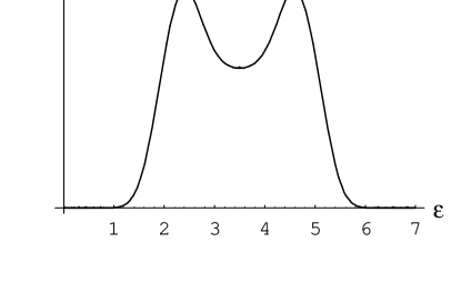
Figure 1: Degeneracy of the two string system, in the broken-equipartition regime. The total energy of the system is $\frac{7}{(\alpha^{\prime})^{1/2}}$.

In this last regime equipartition is broken. Another way to observe this behaviour is by looking at the density of states of the two string gas obtained through convolution, and comparing it with the single string one. As the energy grows both functions give the same termodynamics in the sense that for the same big total energy both densities of states produce the same thermal properties, see Fig.3. In the next section we will find $T$ as a function of the energy. The same behaviour can be seen for a three string gas, as in Fig.2.

Figure 2: Degeneracy of the three string system with a total energy $\frac{10}{(\alpha^{\prime})^{1/2}}$.

One could wonder whether the fat (energetic) string would eventually capture all the energy while the others disappear. To this purpose we can make a simple calculation for the two-string example. We start from a concrete configuration of the gas with a total energy $E$. We assume that one of the strings is energetic enough to approximate well its density of states by the leading behaviour at high energies, and the other will be supposed to be in the massless range. The degeneracy of this configuration would be

$$\omega(E,{\cal E})\propto{\cal E}^{24}(E-{\cal E})^{-27/2}e^{\beta_{H}(E-{\cal E})}$$ (27)

where ${\cal E}$ is the energy of the light string. As a function of ${\cal E}$, $\omega(E,{\cal E})$ will increase if

$$\frac{24}{{\cal E}}-\beta_{H}+\frac{27}{2(E-{\cal E})}>0$$ (28)

and decrease otherwise. For a given value of ${\cal E}$ if $\omega(E,{\cal E})$ grows (lessens) the most probable value of ${\cal E}$ would be bigger (smaller) than the considered one. Note that if ${\cal E}<\frac{24}{\beta_{H}}$ then the condition will always be satisfied no matter how energetic the other string is. This means there will always be a small string of at least that critical energy. This simple model allows us to induce that in a string gas there will exist, as the total energy becomes bigger, a very energetic string and a low energetic string sea. In the next section we will make another explanation of this fact for a $n$-string gas using its thermal properties.

6 Thermodynamics

We start from some basic definitions of thermodynamical magnitudes in the microcanonical ensemble:

$$T^{-1}(E) = \frac{\partial\log(\Omega(E))}{\partial E}=\frac{\Omega^{\prime}(E)}{\Omega(E)}$$

$$C_{V}^{-1}(E) = \frac{\partial T(E)}{\partial E}$$ (29)

The expressions above for the temperature clarify the problem of the infinite volume. Writing $\Omega(E)$ as a series in $n$ , the temperature becomes

$$T(E)=\lim_{V\rightarrow\infty}\frac{\sum_{n=1}^{N}{\cal A}(n,E)V^{n}}{\sum_{n=1}^{N}{\cal A}^{\prime}(n,E)V^{n}}=\frac{{\cal A}(N,E)}{{\cal A}^{\prime}(N,E)}.\vspace*{0.5cm}$$ (30)

Then the only term one has to consider in order to calculate the thermal properties is the last one, that is the term with the biggest $n=N$. In other words, we are taking $V$ to infinity irrespective of the value of $E$.

In general the specific heat is a linear function of the number of subsystems and so it is sometimes useful to define a specific heat per subsystem, as follows

$$\tilde{C}_{V}^{-1}(u)=\frac{\partial T(u)}{\partial u}=\frac{N}{C_{V}(E)}$$ (31)

We have computed numerically the temperature for the single and the two-string gases. The results are shown in Fig.3 and Fig.4.

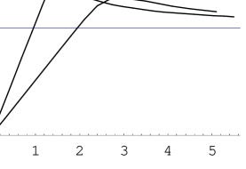
Figure 3: Temperature of the one and two-string gases with the same total energy. Both systems have $E=2u$, where $u$ is the energy per string in the two-string case.

Figure 4: Temperature of the single and two string gases with the same energy per string.

Some important features come up. First of all, one sees that both systems go from the low energy regime to the high energy one through a maximum. The explanation for the single string is clear; when the system is in the low energy regime everything happens like in a particle gas, that is, the specific heat is finite, positive and constant. However, when the amount of energy is enough for the string to reach the Planck mass level, this energy is in part used to create the mass and not to increase the kinetic energy so the temperature tends finally to decrease. In a system with only two levels the temperature would increase again because after creating the mass the rest of the energy is employed in accelerating the particles, and so elevating the temperature. In our system there is an infinite number of highly degenerated mass levels, each one more than the previous, such that the energy will always be used to create ever more massive fields. That is why the temperature gets lower.

To calculate the high energy limit of the temperature, it is useful to approximate the density of states by the leading term in (18). It gives the well-known expression for the temperature:

$$T=\frac{E}{\beta_{H}E-\frac{27}{2}}$$ (32)

which tends to $T_{H}$ when $E\rightarrow\infty$.

In the two-string gas the behaviour is practically the same except for the fact that the maximum occurs at a lower temperature. This comes from the growth of the number of energy levels that are accesible to each string when it borrows some energy from the other. The deviation from equipartition is responsible for the cooling of the gas. The maximum appears approximately at a total energy $2u_{0}$, that is, when each string has the critical energy assuming equipartition. In both figures, we can see the two different regimes of the gas. When the energy is large, the two-string gas behaves nearly as a single string with all the energy, just as the energy distributions had predicted.

It is possible to generalize this high energy behaviour for a multiple string gas using the degeneracy of a configuration similar to the one in eq.(27). Let us suppose we have $N$ strings in the low energy regime and a fat one sharing a total energy $E$:

$$\omega(E,u)=\Omega_{N}(Nu)\Omega_{1}(E-Nu).$$ (33)

Then taking the derivative with respect to $u$, which is now the density of energy per string, it is easy to see that $\omega(E,u)$ will increase with $u$ only if $T_{fat}>T_{sea}$. Since when the energy of the energetic string grows, the value of $T_{fat}$ tends to the Hagedorn temperature $T_{H}$, then in this situation the temperature of the other strings will also be $T_{H}$. It seems that the string sea plays the rôle of a great heat bath in which the fat string is contained.

We can put together all the information we have: the single and two-string gases density of states, the energy distribution of any number of strings and other physical hints that allow us to present a pretty realistic model.

Let us imagine we have an infinite universe filled with a very rarefied and low energetic string gas. Let us suppose we are able to introduce more and more energy at the same time that we observe the system evolution. It would begin behaving like a particle gas with a positive specific heat per particle. As the density of energy per string grows, the strings are able to occupy more and more massive states, increasing the specific heat, as we have already explained for the two-string gas. At a certain value of the energy, the temperature reaches the Hagedorn one. Until that point, equipartition applies, but if we tried to increase slightly the energy of the gas, the probable distribution would change in such a way that a single string would come out from the gas and absorb all the energy added. In other words, the most probable number of strings absorbing energy is one.

It is very important to note that since we are considering an infinite volume universe, the number of strings and the total energy of the system are also infinite. Hence, it is only possible to deal with densities per unit volume or per subsystem. Both densities are simply related at least in the particle case, as we have seen before. For energies higher than the critical one, the density of strings is always the same as no energy is absorbed or emitted by the string sea.

It is clear that the fat string appears with an already infinite amount of energy, and it can only exist being infinitely energetic. Therefore its temperature will always be Hagedorn. We find no negative specific heat for any value of the energy. We do, however, find a divergent specific heat for energies per string bigger than a certain critical point (approximately $u_{0}$). This is not a surprise because when a finite maximum temperature of a system is expected, the specific heat diverges. For example, the only difference with the open string case is that this divergence in $C_{V}$ appears at a finite value of $u$. One could wonder whether this divergence appears abruptly or in a continuous way. We have seen that when one makes one convolution, the maximum temperature gets lower. The corresponding maxima are smooth and no discontinuity in $T$ is observed. That is why we think that the natural extrapolation for a large number of convolutions is that the system will keep this behaviour, and the maximum, that we already know is Hagedorn, will be reached smoothly. We present a tentative plot of the qualitative thermal behaviour of the system in Fig.5.

Figure 5: Tentative plot of temperature versus energy per string

7 Conclusions

In this paper we have revisited the thermal behaviour of a bosonic string gas in the microcanonical ensemble. We have introduced some mathematical tools which seem to be useful to make the inverse Laplace transorm. The rôle of the analytical parts have manifested as important to grant the convergence of the series which allowed us to account for the quantum statistics effetcs in the single string density of states at high energies. However, the physical range of application of (18) is not known because it does not contain the infrared part of the free energy associated in the $\beta$ complex plane with singularities on the imaginary axis. On the other hand this expression is completely useless in order to calculate the multiple string density. This is due to the need of the convolution theorem, that we see as the most physical way to compute the multiple string case. This enforces us to try to compute a valid expression for the density of states for the whole energy range. We succeeded making that for the single string and, by application of the convolution theorem, we observe a behaviour from which we induce that for infinite volume, summing up over an infinite number of subsystems, no negative specific heat phase appears. On the contrary, at high energies, we have a system which absorbs any amount of energy without increasing its temperature, so the limiting temperature $T_{H}$, is actually a maximum one for the universe. What seems to be clear to us is that the description of this phase as one with, not only a fat string, but also with a sea of a large number of low-energy strings is not adequate to the degrees of freedom we have at hand. It is only the result of trying to enforce a description of these degrees of freedom in terms of strings when no equilibrium is posible among them as subsystems. To be more concrete, we do not believe an alternative description of these degrees of freedom should change the fact that, perturbatively at least, Hagedorn is the maximum temperature of the system.

The study we have presented can be easily extended to Superstrings. The next refinement of the thermodynamics would be considering non-perturbative effects as D-Instantons. A calculation of the influence of these effects on the one loop free energy has been done in [2], where the authors have also obtained an expression for the high energy density of states for this case. This type of calculation is along the lines of the works in [4] in which no infinite volume limit is actually taken, but what they do amounts to taking a high energy limit for each $\Omega_{n}$ in (10) then substituting the energy dependence for that of the single string in such a way that finally they approximate $\Omega(E)$ by the asymptotic expression for the single string density times the exponential of $V$. So no limit in $V$ is in fact needed. In this way no phase transition can then be captured because no critical limit is taken. Obviously this procedure is completely different from ours ab initio.

We believe that to include D-Instantons effects in our picture, it is necessary to compute once more the complete density of states for the single string with this corrections, and then, by convolution, obtain the multiple string gas.

References

-
[1]
R.Hagedorn Nuovo Cimento Supp.3 147 (1965)
S.Frautschi Phys. Rev. D3 2821 (1971)
R.Carlitz Phys. Rev. D5 3231 (1972)
N.Cabbibo and G.Parisi Phys. Rev. B59 67 (1975) - [2] J.Barbón and M.A. Vázquez Mozo. CERN-TH/96-361 and IASSNS-96/127
- [3] M.Green Phys. Lett. B354 271 (1995), hep-th/9504108.
-
[4]
N.Deo, S.Jain and C.-I.Tan Phys. Rev. D45 3641 (1992)
M.Axenides, S.D.Ellis and C.Kounnas Phys. Rev. D37 2964 (1988)
M.McGuigan Phys. Rev. D38 552 (1988) - [5] E.Álvarez Nucl.Phys. B269 596 (1986)
- [6] G.Horowitz Comm. Math. Phys. 89 117 (1983)
-
[7]
B. McClain B. Roth Comm. Math. Phys 111 538 (1987)
D.Kutasov and N.Seiberg Nucl. Phys. B358 600 (1991)
K.H.O’Brien and C.-I.Tan Phys. Rev. D36 1184 (1987)
E. Álvarez and M.A.R. Osorio Nucl. Phys. B304 327 (1988)
M.A.R. Osorio Int. J. Mod. Phys.A7 4275 (1992) - [8] M.A.R Osorio and M.A. Vázquez Mozo Phys. Lett. B280 21 (1992), Phys. Rev. D47 3411 (1993)
- [9] E.Álvarez and M.A.R.Osorio Phys. Rev. D36 1175 (1987)
- [10] R.H.Brandenberger and C.Vafa Nucl. Phys. B316 391 (1988)
- [11] A.Erdélyi (Editor) Tables of integral transforms. Vol I (McGraw-Hill Book Company, Inc. New York 1954)