Abstract

The study of the convergence of power series expansions of energy eigenvalues for anharmonic oscillators in quantum mechanics differs from general understanding, in the case of quasi-exactly solvable potentials. They provide examples of expansions with finite radius and suggest techniques useful to analyze more generic potentials.

Key words: Perturbative expansions, anharmonic oscillators, quasi-exactly solvable potentials, Bender-Dunne polynomials.

1 Introduction

Let me summarize some of the most relevant features of perturbative expansions for eigenvalues in one-dimensional quantum mechanics. Let us consider the Schrödinger equation

$$\left[-\frac{\partial^{2}}{\partial x^{2}}+\frac{x^{2}}{4}+\lambda V(x)\right]\psi_{k}(x)=E_{k}\,\psi_{k}(x)$$ (1.1)

where the harmonic oscillator is perturbed by a higher order even polynomial $\lambda V(x)=\lambda p(x^{2})$ and $k$ is the number of zeros of the wave function .
In well known papers C.Bender and T.T. Wu [1] and B.Simon [2] studied the quartic anharmonic oscillator $p(x^{2})=x^{4}$ . The former authors [1] evaluated a large number of terms of the perturbative series

$$E_{k}(\lambda)=(k+1/2)+\sum_{n=1}^{\infty}\lambda^{n}E_{k}^{(n)}$$ (1.2)

of the lowest energy eigenvalues $E_{k}(\lambda)$, $k=0,1,..$ and discussed the occurrence of singularities in the complex $\lambda$ plane. It was found that for any energy level $E_{k}(\lambda)$ there exist infinitely many points $\bar{\lambda}$ , which are extrema of square root branch singularities , the extrema accumulate at the origin in the complex $\lambda$ plane and each value $\bar{\lambda}$ correspond to the crossing between pairs of energy levels

$$E_{n}(\bar{\lambda})=E_{m}(\bar{\lambda})$$ (1.3)

These features prevent a non vanishing radius of convergence for the perturbative expansion of any energy eigenvalue (1.2). The second author [2] confirmed these results, by using Hilbert space methods. Analogous occurrence of infinitely many singularities with accumulation point at the origin, for any energy level, was found if the quartic monomial $\lambda\,x^{4}$ was replaced by a higher order monomial $\lambda\,x^{2n}$, $n>2$ [2]. T.Banks and C.Bender [3] also studied the anharmonic oscillator with a general polynomial potential (of even parity)

$$H=-\frac{\partial^{2}}{\partial x^{2}}+\frac{x^{2}}{4}+g\left[\left(\frac{x^{2}}{2}\right)^{N}+a\left(\frac{x^{2}}{2}\right)^{N-1}+b\left(\frac{x^{2}}{2}\right)^{N-2}+...\right]$$ (1.4)

The $k-th$ energy level has a perturbative expansion

$$E_{k}(g)=k+\frac{1}{2}+\sum_{n=1}^{\infty}c_{n}^{(k)}(a,b,..)g^{n}$$

They found that the large order behaviour of the coefficients $c_{n}^{(k)}(a,b,..)$ is given by

$$\frac{c_{n}^{(k)}(a,b,..)}{c_{n}^{(k)}(0,0,..)}\sim e^{a/(N-1)}\left[1+O(\frac{1}{n})\right]$$ (1.5)

Then the singularities of $E_{k}(g)$ closest to the origin in the complex $g$ plane are controlled by the highest order monomial $g(x^{2}/2)^{N}$ whereas the next order monomial $ga(x^{2}/2)^{N-1}$ only results in a constant factor and the next order monomial $gb(x^{2}/2)^{N-2}$ affects the corrections of order $O(1/n)$ with respect to the previous result.
For some decades it was believed that any formal Taylor expansion of energy eigenvalues of an anharmonic potential, with any polynomial perturbation (of degree higher than quadratic) would have a vanishing radius of convergence. It was recently found that for the class of models known as quasi exactly solvable potentials, a number of energy levels have a perturbative expansion with finite radius of convergence [4]. The singularities of these energy levels still correspond to level crossing, yet these are a finite number. Quantum mechanics being a $(0+1)$ dimensional quantum field theory, it would be exciting to find similar convergence in higher dimensional models of quantum field theory.
Further references to extensive investigations on the divergence of the perturbative expansion in quantum mechanics and in quantum field theory may be found in [5] and [6].
It is clear that quasi-exactly solvable models have convergent perturbative expansions for a finite number of energy eigenvalues because those eigenvalues are decoupled from the rest of the spectrum. Yet this property is so peculiar, that it is interesting to have a pattern of the radius of convergence as function of the parameters. This is evaluated in sect.2, in an algebraic exact fashion, for a simple sequence of potentials. It also seems that quasi-exactly solvable potentials provide efficient tools to investigate the possibility of convergence for generic potentials, when these are summed in a fashion similar to quasi-exactly solvable models. This analysis is presented but not completed in sect.3.

2 Quasi-exactly solvable potentials.

The generic conclusion of divergence of perturbative expansion does not hold in the case of quasi-exactly solvable potentials. This is clearly stated in the book [4]. In this section it will be exhibited by the evaluation of the radius of convergence in a sequence of cases.
The simplest class of quasi-exactly solvable potentials corresponds to the one-dimensional quantum sextic oscillator model with hamiltonian

$$H_{M}=-\frac{\partial^{2}}{\partial x^{2}}+[b^{2}-a(4M+3)]x^{2}+2abx^{4}+a^{2}x^{6}$$ (2.1)

where $a$ is positive, $b$ is real, $M$ is a non-negative integer ($M=0,1,..)$ For sake of a simpler exposition, let us choose $b=1$ (which is a generic value). It can be shown that the eigenvalue equation

$$\left[-\frac{\partial^{2}}{\partial x^{2}}+[1-a(4M+3)]x^{2}+2ax^{4}+a^{2}x^{6}]\right]\psi_{k}(x)=E_{k}\psi_{k}(x)$$ (2.2)

where $\psi_{k}(x)$ is square integrable, has the lowest part of the spectrum corresponding to the even wave functions, which may be computed in closed form in algebraic way. That is, the first $M+1$ even wave functions $\psi_{2k}(x^{2})$, $k=0,1,..M$ are

$$\psi_{2k}(x^{2}) = e^{-\frac{x^{2}}{2}-\frac{ax^{4}}{4}}\prod_{i=1}^{M}\left(\frac{x^{2}}{2}-\xi_{i}\right)=$$ (2.3)

$$= e^{-\frac{x^{2}}{2}-\frac{ax^{4}}{4}}\sum_{n=0}^{M}\frac{(-1)^{n}P_{n}(E)}{(2n)!}x^{2n}$$ (2.4)

where $\xi_{1},\dots,\xi_{M}$ are real numbers satisfying the system of $M$ algebraic equations

$$\sum_{k=1,k\neq i}^{M}\frac{1}{\xi_{i}-\xi_{k}}+\frac{1}{4\xi_{i}}-1-2a\xi_{i}=0$$ (2.5)

Each of the $M+1$ solutions of the set $\{\xi_{i}\}$ is characterized by having $k$ of the numbers $\{\xi_{i}\}$ positive and the remaining $M-k$ being negative. It provides one of the $M+1$ computable energy eigenvalues:

$$E_{2k}=(4M+1)+8a\sum_{i=1}^{M}\xi_{i}$$ (2.6)

and the ground state corresponds to the solution where all the numbers $\{\xi_{i}\}$ are negative. The eq.(2.5) has the familiar form of a saddle point equation for random matrix models and the promising relations between quasi exactly solvable models and random matrix models are just beginning to be explored [7] [8].
The system (2.5) and eq.(2.6) imply that for fixed non negative integer $M$, the $M+1$ eigenvalues of the lowest even wave functions are the roots of a polynomial equation of order $M+1$ which may be obtained by techniques of symmetric functions. It is however easier to obtain them by inserting the ansatz (2.3) in the eigenvalue equation (2.2) bypassing the evaluation of the set $\{\xi_{i}\}$. For example, the five polynomial equations which correspond to the values $M=0,1,..,4$ are

$$E-1=0$$

$$E^{2}-6E+5-8a=0$$

$$E^{3}-15E^{2}+(59-64a)E+(192a-45)=0$$

$$E^{4}-28E^{3}+(254-240a)E^{2}-(812-2592a)E+(585-4656a+2880a^{2})=0$$

$$E^{5}-45E^{4}+10(73-64a)E^{3}-114(45-128a)E^{2}+$$

$$\qquad 128(\frac{14389}{128}-709a+368a^{2})E-128(\frac{9945}{128}-984a+1776a^{2})=0$$ (2.7)

The second ansatz for the wave function (2.4) is very useful to derive the wave function because one immediately finds a three term recursion relation for the coefficients $P_{n}(E)$

$$(E-4k-1)P_{k}=P_{k+1}-8ak(2k-1)(k-1-M)P_{k-1}$$ (2.8)

with

$$P_{0}=1\;,\qquad P_{1}=E-1$$ (2.9)

The coefficient $P_{n}(E)$ is then a polynomial in $E$ of order $n$. The condition that $P_{M+1}(E)=0$ leads to the algebraic equation for $E$ of degree $M+1$ (the lowest ones being eq.(2.7) ). This condition and the recursion relation eq.(2.8) imply that all $P_{k}(E)$ with $k>M$ vanish. The finite set of non-vanishing polynomials $P_{n}(E)$ is a set of weakly-orthogonal polynomials, recently discussed by several authors [9], [10], [11]. The papers [10], [11] show that a set of weakly-orthogonal polynomials occur in any quasi-exactly solvable model and they exhibit the discrete weight function $\omega(E)=\sum_{k=0}^{M}\omega_{k}\delta(E-E_{k})$ for which

$$\int{P_{n}(E)P_{m}(E)\omega(E)dE}=h_{n}\delta_{n,m}$$ (2.10)

The roots of the polynomial eqs.(2.7), $P_{M+1}=0$, $M=0,1,...$, determine the even lowest energy eigenvalues $E_{0}(a),\,E_{2}(a),\,..,E_{2M}(a)$. The singularities of the function $E_{2k}(a)$ closest to the origin, in the complex plane of the variable $a$ provide the radius of convergence of the perturbative expansions

$$E_{2k}(a)=1+4k+\sum_{n=1}^{\infty}d_{n}^{(k)}a^{n}$$ (2.11)

The singularities only occur for the values ${\overline{a}}$ such that $E_{2k}({\overline{a}})$ is a multiple root and may be found by examining the solution of the system

$$P_{M+1}(a,E)=0=\frac{\partial}{\partial E}P_{M+1}(a,E)$$ (2.12)

For instance, for $M=2$,

$$P_{3}(E)=E^{3}-15E^{2}+(59-64a)E+(192a-45)=0$$ (2.13)

defines, in closed form, the three energy levels $E_{0}(a),\,E_{2}(a),\,E_{4}(a)$, and their perturbative expansions may be easily evaluated at arbitrary order

$$E_{0}(a)=1-4a-2a^{2}+4a^{3}+\frac{1}{2}a^{4}-11a^{5}+\frac{39}{4}a^{6}+\frac{57}{2}a^{7}-\frac{2235}{32}a^{8}-$$

$$\frac{563}{16}a^{9}+\frac{21809}{64}a^{10}+...$$ (2.14)

$$E_{2}(a)=5-8a+32a^{2}-160a^{3}+1024a^{4}-7552a^{5}+59904a^{6}-497664a^{7}+$$

$$+4276224a^{8}-37697536a^{9}+339042304a^{10}+...$$ (2.15)

$$E_{4}(a)=9+12a-30a^{2}+156a^{3}-\frac{2049}{2}a^{4}+7563a^{5}-\frac{239655}{4}a^{6}+$$

$$+\frac{995271}{2}a^{7}-\frac{136836933}{32}a^{8}+\frac{603161139}{16}a^{9}-\frac{21698729265}{64}a^{10}+...$$ (2.16)

The singularities of $E_{0}(a)$ , eq.(2.13), occur for the three values ${\overline{a}}$

$${\overline{a}} = [3(11+64\sqrt{3})^{1/3}-7-\frac{69}{(11+64\sqrt{3})^{1/3}}]/64\sim-0.09445127$$

$${\overline{a}} \sim -0.116837\pm 0.389587\,i$$ (2.17)

where the above pair of complex conjugate values are the roots of

$${\overline{a}}^{2} + \frac{7406+1587\rho+(33-192\sqrt{3})\rho^{2}}{33856}{\overline{a}}+\frac{\rho}{69+7\rho-3\rho^{2}}=0$$

$$\rho \equiv (11+64\sqrt{3})^{1/3}$$ (2.18)

It is easy to check that the closest, real negative value of ${\overline{a}}$ , (2.17), corresponds to the radius of convergence of the perturbative expansions of both the levels $E_{2}(a)$ and $E_{4}(a)$, (2.15) and (2.16), and may be interpreted as the value of $a$ corresponding to the crossing $E_{2}({\overline{a}})=E_{4}({\overline{a}})$ , while the couple of complex conjugate values (2.18) correspond to the radius of convergence of the perturbative expansion of the ground level $E_{0}(a)$ , (2.14). It is remarkable how easily this situation generalizes for all integer values of $M$. The $M+1$ roots of the polynomial equation $P_{M}(E)=0$ define the $M+1$ energy eigenvalues $E_{0}(a),\,E_{2}(a),\,...E_{2M}(a)$; the system (2.12) leads to a polynomial equation in the variable $a$ of degree $M(M+1)/2$. Its $M(M+1)/2$ roots in the complex $a$ plane are in one-to-one correspondence with the possible level crossing among pairs of eigenvalues

$$E_{2r}({\overline{a}})=E_{2s}({\overline{a}})$$ (2.19)

All these singular values were examined, for the cases $M=1$ up to $M=7$, beginning with the values ${\overline{a}}$ with the smallest modulus. For any $M$ examined, the first value ${\overline{a}}$ occurs on the real negative axis in the $a$ complex plane, it corresponds to crossing of the two highest eigenvalues considered (for $M=7$ it is $E_{12}({\overline{a}})=E_{14}({\overline{a}})$) thus providing the radius of convergence of their perturbative expansions (2.11). Singular values ${\overline{a}}$ with larger modulus describe level crossing between pairs of intermediate levels. Only the $M$ values ${\overline{a}}$ with larger modulus describe level crossings of the ground state level with the other $M$ levels. The radius of convergence of the perturbative expansion of the ground level $E_{0}(a)$ is determined by a couple of complex conjugate values of ${\overline{a}}$ with the smallest modulus in this last group of $M$ values ${\overline{a}}$. This analysis is confirmed by the study of the period of oscillations of the coefficients in the perturbative expansion of $E_{0}(a)$.

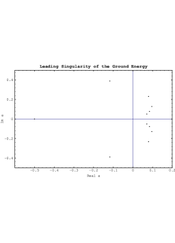
Figure 1:

Fig.1 shows a sequence of points ${\overline{a}}$ in the complex $a$ plane. The point ${\overline{a}}=-1/2$ corresponds to the only singularity of the ground state eigenvalue $E_{0}(a)=3-2\sqrt{1+2a}$ of the potential (2.2) with $M=1$. Moving clockwise in the upper half plane, there are points corresponding to the singularity of $E_{0}(a,M)$ closest to the origin, for the cases $M=2,3,..,6$. One sees that the radius $r_{M}$ of convergence decreases as $M$ increases.

3 Softly broken quasi-exact solvability

The analysis of quasi-exactly solvable models is useful for more general polynomial potentials, where the couplings do not obey the constraints of quasi-exact solvability. Let us consider the hamiltonian with a generic sextic potential

$$H=-\frac{\partial^{2}}{\partial x^{2}}+{\cal V}(x)=-\frac{\partial^{2}}{\partial x^{2}}+\alpha x^{2}+\beta x^{4}+\gamma x^{6}$$ (3.1)

with $\gamma>0,\,\alpha$ and $\beta$ real. By choosing

$$a=\sqrt{\gamma}\,,\;b=\frac{\beta}{2\sqrt{\gamma}}\,,\;M=\frac{1}{4}[\frac{1}{\sqrt{\gamma}}(\frac{\beta^{2}}{4\gamma}-\alpha)-3]$$ (3.2)

the hamiltonian (3.1) reproduces the quasi-exactly solvable model (2.1), but now $M$ is real, rather than a non negative integer. In this Section, I study the perturbation theory for the eigenvalues of this hamiltonian, by keeping $b$ and $M$ fixed, in series of powers of the coupling $a$. This is just a specific way to do perturbation theory for the generic sextic potential (3.1). For simplicity let us fix again $b=1$, which is a value with no special meaning, and let us choose the (formal) ansatz for the even parity wave function

$$\psi(x^{2}) = \phi(a,x^{2})\;e^{-\frac{x^{2}}{2}-\frac{ax^{4}}{4}}$$

$$\phi(a,M,x^{2}) = \sum_{n=0}^{\infty}\frac{(-1)^{n}P_{n}(E,a,M)}{(2n)!}x^{2n}$$ (3.3)

The eigenvalue eq.(1.1) implies the recursion relations

$$P_{n}(E,a,M)=(E-4n+3)P_{n-1}(E,a,M)-\lambda_{n}P_{n-2}(E,a,M)$$

$$\lambda_{n}\equiv 8a(n-1)(2n-3)(M+2-n)$$ (3.4)

Since $M$ is not a non-negative integer, the number of non-vanishing polynomials $P_{n}(E,a,M)$ is infinite. However $\lambda_{n+1}>0$ only for $n<M+1$ so the system of infinite polynomials $P_{n}(E,a,M)$ is not an orthogonal systems with respect to a non-negative Stieltjes measure [12]. Still the recursion relations (3.4), are a powerful tool for the perturbative analysis of the generic sextic potential (3.1). The first few polynomials $P_{n}(E,a,M)$ are

$$P_{0}(E,a,M)=1\;;\;P_{1}(E,a,M)=E-1$$

$$P_{2}(E,a,M)=E^{2}-6E+5-8aM$$

$$P_{3}(E,a,M)=E^{3}-15E^{2}+(59-56aM+48a)E+(120aM-48a-45)$$

$$P_{4}(E,a,M) = E^{4}-28E^{3}+(254+288a-176aM)E^{2}-(812+2112a-1568aM)E+$$

$$+ (585+1824a-2160aM-1920a^{2}M+960a^{2}M^{2})$$

$$P_{5}(E,a,M) = E^{5}-45E^{4}+10(73+96a-40aM)E^{3}-(5130+17088a-7920aM)E^{2}$$ (3.5)

$$+ (14389+77376a+32256a^{2}-42032aM-50304a^{2}M+13504a^{2}M^{2})E-$$

$$(9945+61248a+32256a^{2}-46800aM-124032a^{2}M+43200a^{2}M^{2})$$

The energy eigenvalues are the roots of the polynomial equation such that the Hill determinant [13] [14] $D(E)$ vanishes

$$D(E)=\pmatrix{1-E&1&0&0&0&0&..\cr 8Ma&5-E&1&0&0&0&..\cr 0&48(M-1)a&9-E&1&0&0&..\cr 0&0&120(M-2)a&13-E&1&0&..\cr 0&0&0&224(M-3)a&17-E&1&..\cr 0&0&0&0&..&..&..\cr}$$

If the infinite matrix is truncated at order $N$, its determinant $D_{N}(E)$ is solution of the recurrence relation

$$D_{N+1}(E)=(4N+1-E)D_{N}(E)-8aN(2N-1)(M+1-N)D_{N-1}(E)$$ (3.6)

therefore $D_{N}(E)=(-1)^{N}\,P_{N}(E,a,M)$.
Let us insert the formal expansion $E_{0}(a)=1+\sum_{n=1}^{\infty}d_{n}a^{n}$, where $d_{n}$ are unknown variables, into the polynomial $P_{k}(E,a,M)$ and expand in powers of the coupling $a$

$$P_{k}(E=1+\sum_{n=1}^{\infty}d_{n}a^{n},a,M)=\sum_{n=0}^{\infty}c_{p}^{(k)}[{d},M]a^{p}$$ (3.7)

The coefficients $c_{p}^{(k)}[{d},M]$ depend on $d_{r}$ up to $r=p$ and vanish if $d_{r}$ are the perturbative coefficients of the expansion of the ground energy eigenvalue, and $k>p$. This basic property of the polynomials $P_{k}(E,a,M)$ allows to translate the eqs.(3.4) into recursion relations for the coefficients $c_{p}^{(k)}[{d},M]$, which allow the exact evaluation of $d_{n}(M)$ in an automated way. The perturbative expansion of other, even and odd, energy eigenvalues may also be performed with small changes [13] .
For instance one obtains for the ground state eigenvalue (to save space, I only quote the term of order $a^{20}$ ):

$$E_{0}(a)=1-2Ma-M(2M-3)a^{2}-M(4M^{2}-15M+12)a^{3}-M(40M^{3}-$$

$$264M^{2}+516M-297)a^{4}-M(28M^{4}-279M^{3}+948M^{2}-\frac{5229}{4}M+612)a^{5}-...$$

$$..M[14739534473769094441397440311/131072 - 15258905673899527021780026567/32768\,M+$$

$$1784658246229507614806783961/2048\,M^{2} - 507856798436368302225354717/512\,M^{3}+$$

$$6366289590321020410675505193/8192\,M^{4} - 114826346450120328738858675/256\,M^{5}+$$

$$25467941727184707982391625/128\,M^{6} - 17860681260918574154980695/256\,M^{7}+$$

$$5045855866084769519143395/256\,M^{8} - 290745864268625747137893/64\,M^{9}+$$

$$13767162352069961178387/16\,M^{10} - 2148046668981444052251/16\,M^{11}+$$

$$275387290187286326553/16\,M^{12} - 1798144942712999139\,M^{13}+$$

$$150720427787130918\,M^{14} - 9879984325256823\,M^{15}+$$

$$972416331565443/2\,M^{16} - 16789635150822\,M^{17}+$$

$$359298964716\,M^{18} - 3534526380\,M^{19}]\,a^{20}+...$$ (3.8)

I checked the coefficients $d_{n}(M)$ up to $n=11$ by performing the the regular perturbative expansion for $log[\psi(x)]$, a rather efficient method for not very large order. Simple checks of the coefficients $d_{n}(M)$ for higher orders are provided by evaluating them for positive integer values of $M$, where they reproduce the easily obtainable expansions of eqs.(2.7).

4 Concluding remarks.

The properties of anharmonic oscillators perturbed by polynomial potentials which correspond to quasi-exactly solvable models are peculiar. The perturbative expansions of the eigenvalues have a finite radius of convergence, which evades the general situation. In Sect.3, it was indicated that properties of quasi-exactly solvable models may be useful to the study of more general non-quasi-exactly solvable models. More specifically, one may evaluate in exact, automated way, the perturbative expansions of energy eigenvalues. It would be very interesting to know whether the radius of convergence of these expansions collapses to zero, as soon as $M$ differs from a positive integer, or there exist other real values of $M$ where such radius is finite. If this were the case, quasi-exactly solvable models would have the additional merit of suggesting ways of dealing with polynomial perturbations. The answer to this question requires standard methods of analysis of coefficients of the perturbative expansions which I hope to report in a future work.
After the present letter was completed, I saw the recent paper by M.Znojil [15] , which addresses similar issues, with different techniques and an old letter by A.V.Turbiner and A.G.Ushveridze [16] where a subset of the investigation here reported in Sect.2 was performed.

5 Acknowledgements

I thank G.Burgio, M.P.Manara,P.L.Rigolli for useful discussions, R.De Pietri for help with programming with Mathematica, P.Butera for reading the manuscript and A.G.Ushveridze who started my interest in quasi-exactly solvable models.

References

- [1] C.M.Bender and T.T.Wu, Phys.Rev.184 (1969) 1231 and Phys.Rev.D7 (1973) 1620.
- [2] B.Simon, Ann.of Phys.58 (1970) 76.
- [3] T.I.Banks and C.M.Bender, J.Math.Phys.11 (1970) 796.
- [4] A.G.Ushveridze, Quasi-Exactly Solvable Models in Quantum Mechanics, Inst.of Physics 1994.
- [5] G.A.Arteca, F.M.Fernandez,E.A.Castro, Large Order Theory and Summation Methods in Quantum Mechanics, Lecture Notes in Chemistry 53, Springer-Verlag 1990.
- [6] J.C.Le Guillou and J.Zinn-Justin, Large-Order Behaviour of Perturbation Theory, CPSC vol.7, (1990), North-Holland.
- [7] G. Cicuta and A.G. Ushveridze, Phys.Lett.A 215 (1996), 167.
- [8] G. Cicuta, S.Stramaglia, A.G. Ushveridze, Mod.Phys.Lett. A 11 (1996), 119.
- [9] C.M.Bender and G.V.Dunne, J.Math.Phys.37 (1996) 6.
- [10] A.Krajewska, A.Ushveridze, Z.Walczak, hep-th/9601088, to appear in Mod.Phys.Lett.
- [11] F.Finkel, A.Gonzalez-Lopez, M.A.Rodriguez, J.Math.Phys. 37 (1996) 3954.
- [12] T.S.Chihara, An Introduction to Orthogonal Polynomials, Gordon and Breach, New York, 1978.
- [13] J.P.Killingbeck, Rep.Prog.Phys.48 (1985) 54.
- [14] C.M.Bender and S.A.Orzag, Advanced Mathematical Methods for Scientists and Engineers, chapt.7.5, McGraw-Hill, 1978.
- [15] M.Znojil, Phys.Lett.A 222 (1996) 291.
- [16] A.V.Turbiner, A.G.Ushveridze, Phys.Lett.A 126 (1987) 181.