OUTP-96-76P
hep-th/9701087
{centering}
Inverse Landau-Khalatnikov
Transformation and Infrared Critical Exponents
of (2+1)-dimensional Quantum Electrodynamics
I.J.R. Aitchison,
N.E. Mavromatos∗
and D. Mc Neill
University of Oxford, Theoretical Physics,
1 Keble Road OX1 3NP, U.K.
Abstract
By applying an inverse Landau-Khalatnikov
transformation, connecting (resummed) Schwinger-Dyson
treatments in non-local and Landau gauges of ,
we derive the infrared behaviour
of the wave-function renormalization in the Landau gauge,
and the associated critical exponents in the normal
phase of the theory (no mass generation). The result agrees
with the one conjectured in earlier treatments. The
analysis involves an approximation, namely an expansion
of the non-local gauge in powers of momenta in the infrared.
This approximation is tested
by reproducing the critical number of flavours necessary
for dynamical mass generation
in the chiral-symmetry-broken phase of .
January 1997
(∗) P.P.A.R.C. Advanced Fellow.
In recent years interest in three- (space-time) dimensional gauge theories has been revived due to their possible connection with novel mechanisms of superconductivity, associated with the recently discovered high-temperature oxides [1]. In the beginning, physicists concentrated their efforts on understanding the superconducting pairing mechanisms; later on it was realized that these materials exhibited unconventional properties even in their normal phase [2]. Such properties suggested deviations from the fermi-liquid behaviour of the cuprates in their normal phase, and much effort has been devoted in the past few years to understanding the physics of the normal phase.
Recently, Landau’s fermi liquid theory was reformulated in terms of the renormalization group, according to which Landau’s fermi liquid corresponds to a theory with a trivial infrared fixed point, i.e. there are no relevant or marginal interactions that can drive the theory to a non-trivial fixed point [3]. In this spirit, the observed deviations from fermi liquid behaviour in the normal phase of the high- cuprates might be explained by the presence of a non-trivial infrared fixed point in the effective low-energy theory describing the physics of the normal state of these materials. There have been works [4] which aimed at studying the interaction of the statistical gauge field ( which simulates the spin interactions in the magnetic scenaria for superconductivity [5]) with the spinon degrees of freedom, in the context of the spin-charge separated phase of the model [6]. It has then been argued that this interaction is marginally relevant, leading to a non-trivial fixed point at low energies. In ref. [7] it has been argued that the holon-gauge interaction is also marginally relevant, leading to a non-trivial infrared fixed point. This interaction was also responsible for the phenomenon of dynamical opening of an energy gap in the holon spectrum, and thus for superconductivity [8].
The model we studied in ref. [7] was a standard model of three-dimensional quantum electrodynamics, with flavours of fermion fields, representing the holons. The number , though, was associated with the angular size of the cells in which we divided the fermi surface of the statistical model, taken to be a circle of radius for simplicity. The continuum theory was obtained by linearizing about points on the surface, the linearization being done by the introduction of quasiparticles as defined in ref. [9]. The concept of the quasiparticles was essential in yielding the correct scaling properties to be used in the renormalization group approach [9, 7]. If is an ultraviolet cut-off in momenta measured above the fermi surface, then the size of the angular cell may be taken to be [7]
| (1) |
where is the magnitude of the three-vector , and is some (infrared) critical exponent to be determined by the renormalization group. The momentum scale is taken to be . Infrared physics is studied by taking the ultraviolet cut-off . The identification of (1) with the inverse of flavour number implies the existence of a running flavour number, i.e. a ‘running’ in theory space of three dimensional gauge theories.
The cell argument given above seems to be too closely tied to the existence of a fermi surface. In ref. [7] we have tried to ask a similar question in a relativistic theory, namely standard quantum electrodynamics in three space-time dimensions (), where there is no fermi radius.
A pleasant outcome of the analysis of ref. [7] was the confirmation of the running of the flavour number arising as a consistent solution of the system of Schwinger-Dyson (SD) equations. This allows a universal treatment of the running of the flavour number. The basic reason why the flavour number in ‘runs’ (or actually ‘walks’ due to slow running [7]) is the fact that the standard coupling constant of has dimensions of . The ultraviolet (UV) behaviour of the theory is trivial, is a superrenormalizable theory, and no UV infinities are encountered. However, the infrared (IR) behaviour is non-trivial, since dynamical mass generation occurs at very low energies [10]. Moreover it is known that the latter phenomenon occurs only below a certain ‘critical’ number of flavours [10, 11]. This already suggests a rôle for the flavour number as a dimensionless coupling constant of , in which case the existence of a critical number of flavours would appear as a critical value of the coupling, above which dynamical mass generation (and hence chiral symmetry breaking) occurs as a strong coupling phenomenon.
Indeed, this interpretation is supported by large-N treatments of SD equations, where the flavour number appears as a dimensionless ratio of a bare coupling constant and a dynamically appearing mass scale . The latter scale was originally defined by demanding finite as , as in standard large-N treatments. However, it was immediately realized [10] that all the momentum loop integrals of in a SD analysis were damped quickly for momentum scales higher than , and hence the latter was considered as a spontaneously appearing mass scale in the problem playing the rôle of an effective UV cut-off. The main point of ref. [7] was then to show that there exists a slow running of the ‘renormalized’ , at intermediate scales of momenta. In terms of the statistical model, the scale may be identified with . In such a case, the infrared physics is equivalent to a large-N approximation, naturally induced in the problem [3, 7]. If there is a non-trivial infrared fixed point, then, the exponent behaves as a critical exponent characteristic of the model. Indeed, the analysis of ref. [7] has shown that the scaling (1) also characterizes the wave-function renormalization of the SD equations for dynamical mass generation in , while the effective static potential behaves as
| (2) |
and, thus, the critical exponent describes the deviation from the Coulombic potential, and therefore from the Landau fermi-liquid (trivial) fixed point [4, 7].
A different set of exponents also characterizes the finite-temperature scaling of the resistivity of the theory, the latter being defined as the response of the system to an externally applied (electric) field. In this article we shall not discuss the finite-temperature analysis. Some preliminary discussion of this important topic may be found in ref. [7], where the temperature is viewed as a sort of finite-size (infrared cut-off) scaling in the problem.
The renormalization of the dimensionful coupling, , and the interpretation of as the effective cut-off scale, are supported by a Wilsonian approach to the Renormalization Group (RG), where the running of a coupling is a consequence of integrating out degrees of freedom, not necessarily associated with UV divergences. However, in our problem, as we discussed in ref. [7], there is an infrared singular behaviour, and in some sense the above-mentioned slow running is associated with it. It is the purpose of this article to elaborate further on this latter point.
The running of and the interpetation of as a cut-off scale in the Wilsonian RG approach, imply an effective running of the dimensionless coupling constant of the problem, i.e. the effective flavour number [7]:
| (3) |
with a momentum scale.
The analysis of ref. [7] was carried out in the Landau gauge and to leading order in expansion. The system of SD equations in this case reads
| (4) | |||||
where is the wave-function renormalization, is the gap function, and the vertex function is . In ref. [7], we made a simple vertex choice , consistent with the Ward-Takahashi identities [12, 13] stemming from gauge invariance.
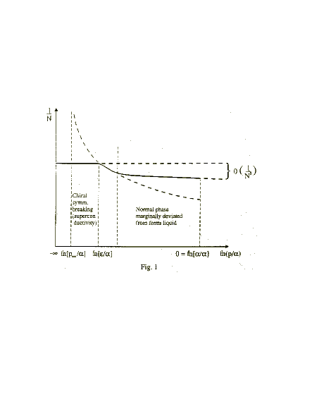
The point of the analysis of ref. [7] was to look for consistent solutions of (4) in the normal phase of the model, where there is no dynamical mass generation. This allows a solution of the wave-function renormalization equation in the SD system, by the bifurcation method [12], i.e. setting in the denominators. Substituting, then, the solution for into the equation for the mass gap one may define an effective ‘running coupling’ [14, 12, 7]
| (5) |
The main result of [7], which improved and extended considerably an earlier treatment in ref. [12] in the dynamical mass generation regime, was to show that (5) runs with the momentum scale (which plays the rôle of an effective RG scale) as in fig. 1. The introduction of an infrared (IR) cut-off scale [12, 7] leads to the appearance of a ‘fixed-point’ structure in the infrared. Removal of the cutoff is a subtle issue and depends on the type of IR cut-off used [7].
Subsequent to the work of [7], an analysis has been performed [15] in the so-called non-local gauge [16], confirming the results of [7] on the slow running of the coupling at intermediate momentum scales , as compared to earlier approximations in a SD analysis of [12], as well as on the existence of an infrared fixed point. The running coupling in the non- local gauge is again defined through the mass gap equation of the SD system, and it turns out to be related to the Fourier transform of the non-local gauge itself [15]:
| (6) |
An important feature of the non-local gauge is that in this gauge the wave-function renormalization is equal to one identically:
| (7) |
Therefore, one would like to study the formal connection of this result to the one derived in the Landau gauge, where the deviation of the wave function renormalization from 1 lead to the running coupling (5) (c.f. fig. 1). In ref. [15] it has been remarked that such a connection is provided by the so-called Landau-Khalatnikov (LK) transformation [16, 17], which by construction leaves the system of SD equations form invariant.
It is the purpose of this short note to apply the (inverse) LK transformation and determine the behaviour of the wave-function renormalization in the infrared regime of the theory in the Landau gauge, starting from quantities evaluated in the non-local gauge. As we shall show, in the absence of an infrared cutoff, where we shall restrict our attention for simplicity, the low-momentum behaviour of the Landau-gauge wave function renormalization is
| (8) |
with playing the rôle of an effective UV cut-off. The exponent appears as a sort of critical exponent characterizing the behaviour of the theory in the infrared. The result (8) has been conjectured in the past, based on either theoretical speculations [18, 13, 19], or in preliminary numerical treatments [11]. The exponent can also be derived from a qualitative study of the renormalization-group running of the effective coupling in the infrared within a SD treatment [7]. In this article we derive this exponent analytically by making a leading-order (infrared) approximation in the LK transformation connecting results in the Landau gauge with those in the non-local gauge. To our knowledge this is the first analytic derivation of a critical exponent in . The presence of this exponent complements the results of refs. [7, 15] about the existence of a non-trivial IR fixed point, and, in view of our statistical interpretation in (1), (2), determines the universality class of the deviations from the fermi-liquid (trivial) fixed point characterizing superconductor models based on [8, 7].
We now proceed to the derivation of . Our starting point will be the LK transformation between the non-local and Landau gauges in the normal phase (no dynamical-mass generation). The fermion propagator in the non local gauge in momentum space reads 111We follow the convention: , .:
| (9) |
which implies that in configuration space
| (10) |
In Landau gauge, on the other hand, the fermion propagator reads:
| (11) |
From the form invariance of the SD equation in the two gauges one may obtain a formal expression of the wave function renormalization in terms of the non-local gauge [16, 15]:
| (12) | |||||
where is related to the Fourier transform of the non-local gauge by:
| (13) |
and is the photon vacuum polarization. In the non-local gauge, in the resummed SD treatment, there is an exact expression for which is given by 222The exactness of the photon polarization is a consequence of the fact that in the non-local gauge , and the vertex function, consistent with Ward-Takahashi identities stemming from gauge invariance, may be taken to be the trivial one, [15].:
| (14) |
Thus, the function is known, once we know the non-local gauge . From the analysis of ref. [15] we have
| (15) |
with the transverse photon propagator given by
| (16) |
as a result of (14). A straightforward computation yields:
| (17) |
and, thus,
| (18) |
In the infrared regime, , where our interest lies, one may expand (18) in powers of :
| (19) |
We wish to evaluate the Fourier transform of (19):
| (20) | |||||
The integral needs regularization in both the ultraviolet and infrared regimes. We choose to regularize the UV infinities by dimensional regularization, introducing the standard RG scale . Using [20]:
| (21) |
one arrives at:
| (22) |
which in the limit yields:
| (23) |
where is the Euler-Macheroni constant.
Next we have to evaluate , which enters the definition of appearing in (12), as a result of the requirement that the coincidence limit of the free fermion propagator is the same in all gauges [16, 17]. To this end, one needs to regularize the coincidence limit . We do so by replacing the argument by , with viewed as our effective UV cut-off scale (in the system of units we are working, we set ). Then we have:
| (24) |
Notice that the UV regularization mass scale disappeared from (24). This is a consequence of the fact that is super-renormalizable in the UV, so only infrared running should emerge, as we shall verify immediately below.
Indeed, we can now give an estimate of the wave-function renormalization in the infrared regime :
| (25) | |||||
Since , in our regularized coincidence limit, is not allowed to go below , the factors are of order one, and the above analysis yields as :
| (26) |
The prefactor in (26) depends on the (bare) flavour number. To get an order of magnitude estimate, we note that for (where dynamical mass generation does not occur, c.f. below) this prefactor is of :
| (27) |
This result has been conjectured [10, 13] but here we proved it analytically, starting from the non-local gauge.
The reader might worry that our result has been obtained on the basis of the approximation (19),which arises from a momentum expansion in the infrared . To substantiate its validity we next perform an analysis of dynamical mass generation in the non-local gauge, upon using (19). As we shall show, in this way one can reproduce very simply the result on the existence of a critical number of flavours, which has been obtained earlier based on more exact treatments [11, 17].
We start our analysis from the expression on the gap function in the non-local gauge 333In this gauge is identical to the mass function. [15]:
| (28) |
with . Expanding the logarithm in the infrared, approximating as
| (29) |
and using as an effective UV cut-off of the momentum integrals, one obtains after performing the angular integrations in (28):
| (30) |
Following standard analysis we can approximate [12]
| (31) |
Upon substituting into (30) we may then convert the integral equation into a differential one for low momenta :
| (32) |
This differential equation should be solved together with the following boundary conditions (consistent with the original integral equation) [10, 8]
| (33) | |||||
The region relevant for dynamical mass generation is ; in this region the differential equation (32) becomes:
| (34) |
Following standard treatments [10, 8], then, it is immediate to see that dynamical mass generation occurs only for flavour numbers smaller than the following critical value:
| (35) |
The number (35), obtained here from an infrared approximation in the expression for the non-local gauge, (29), agrees with more exact treatments [11, 17]. This agreement offers support for the method used here to derive the critical exponents (26) in the normal phase, where a similar infrared approximation, (19), used. Notice also that the result (35) agrees remarkably with that of an earlier treatment [21], incorporating corrections to the SD equations.
The above analysis, then, shows that although the arguments of ref. [13] on the infrared behaviour (26) of the wave-function renormalization were correct, they were not sufficient to destroy the existence of a critical number of flavours for dynamical mass generation, within a resummed- treatment of the SD equations. The existence of a critical number of flavours for dynamical mass generation implies that the renormalization-group diagram of fig. 1 will describe dynamical mass generation in the infrared if and only if the height of the abscissa at the orgin is large enough.
It should be noted at this stage that the presence of an infrared cut-off, which was ignored in this article, will alter the infrared behaviour of the running coupling by cutting off its growth as in fig. 1 [7], and -in the case of dynamical mass generation - will induce an IR-cut-off-dependent [12]. In such a case, one could imagine starting from a non-local gauge with a covariant IR cut-off [15], and applying the inverse LK transformation to reproduce the results of ref. [7] for the infrared behaviour of the wave-function renormalization. It should be stressed, however, that the critical exponent acquires physical meaning, as a quantity characterizing the universality class of the theory (in standard RG language), only after removal of the IR cut-off. We now note that the RG running of the effective coupling in the presence of a covariant IR cut off appears to have discontinuities, which make the removal of the cut off problematic. Such problems have not been resolved yet [7, 15], but we note that such discontinuities might not be so unphysical, given their resemblance to Landau-damping discontinuities appearing in finite-temperature field theories [22],with which a theory with a covariant IR cut off has many things in common [7]. We hope to return to a careful study of such issues in the near future.
The existence of critical exponents, characterizing the infrared behaviour of the model, acquires physical significance when the theory is viewed as a model describing the physics of the planar high- materials, since in that case it characterizes in a universal way the deviations from the fermi-liquid fixed point, and thus is subject to experimental tests [2, 3]. In the present article, the critical exponents have been derived in a rather cavalier way, i.e. by performing a renormalization procedure based on a large-N (resummed) SD analysis. A more exact treatment can be provided by the application of the exact renormalization-group approach due to Wilson [23], appropriately adapted to incorporate large-N treatments. Such a programme, when performed, will yield useful information/verification on the infrared behaviour of the model, and will determine in a more accurate way the associated critical exponents. It may also shed some light on resolving the issue of the discontinuities of the theory with a covariant IR cut-off, found in refs. [7, 15]. Such an analysis is left for future work.
Acknowledgements
We wish to acknowledge useful discussions with M. D’Attanasio, K.-I. Kondo and T. Morris, and to thank K.-I.Kondo for a careful reading of the manuscript. D.McN. wishes to thank P.P.A.R.C. (UK) for a research studentship.
References
- [1] J.G. Bednorz and A. K. Müller, Z. Phys. B64 (1986), 189.
- [2] C.M. Varma et al. , Phys. Rev. Lett. 63 (1989), 7996.
- [3] R. Shankar, Physica A177 (1991), 530; Rev. Mod. Phys. 66 (1994), 129.
- [4] J. Polchinski, Nucl. Phys. B422 (1994), 617; C. Nayak and F. Wilczek, Nucl. Phys. B417 (1994), 359.
- [5] A.L. Fetter, C.B. Hanna and R.B. Laughlin, Phys. Rev. B39 (1989), 9679; Y.H. Chen, B.I. Halperin, F. Wilczek and E. Witten, Int. J. Mod. Phys. B3 (1989), 1001.
- [6] P.W. Anderson, Science 235 (1987), 1196.
- [7] I.J.R. Aitchison and N.E. Mavromatos, Phys. Rev. B53 (1996), 9321; I.J.R. Aitchison, G. Amelino-Camelia, M. Klein-Kreisler, N.E. Mavromatos and D. Mc Neill, preprint OUTP-96-47P, hep-th/9607192.
- [8] N. Dorey and N.E. Mavromatos, Phys. Lett. B250 (1990) 107; Nucl. Phys. B386 (1992), 614.
- [9] G. Benfatto and G. Gallavotti, Phys. Rev. B42 (1990), 9967.
- [10] T.W. Appelquist, M. Bowick, D. Karabali and L.C.R. Wijewardhana, Phys. Rev. D33 (1986), 3704; T.W. Appelquist, D. Nash and L.C.R. Wijewardhana, Phys. Rev. Lett. 60 (1988), 2575.
- [11] K.-I. Kondo and P. Maris, Phys. Rev. D52 (1995), 1212; P. Maris, Phys. Rev. D54 (1996), 4049.
- [12] K.-I. Kondo and H. Nakatani, Progr. Theor. Phys. 87 (1992), 193.
- [13] D.C. Curtis, M.R. Pennington and D. Walsh, Phys. Lett. B295 (1992), 313; M. Pennington and Walsh, ibid. 253 (1991), 246.
- [14] K. Higashijima, Phys. Rev. D29 (1984), 1228.
- [15] K.-I. Kondo, preprint OUTP-96-50P, CHIBA-EP-96;hep-th/9608402.
- [16] L. Landau and I.M. Khalatnikov, Sov. Phys. JETP2 (1956), 69; H. Georgi, E.H. Simmons and A.G. Cohen, Phys. Lett. B236 (1990), 183; T. Kugo and M.G. Mitchard, Phys. Lett. B282 (1992), 162; For an application in see: E.H. Simmons, Phys. Rev. D42 (1990), 2933.
- [17] K.-I. Kondo, T. Ebihara, T. Iizuka and E. Tanaka, Nucl. Phys. B434 (1995), 85.
- [18] T.W. Appelquist and U. Heinz, Phys. Rev. D24 (1981), 2169.
- [19] D. Atkinson, P.W. Johnson and P. Maris, Phys. Rev. D42 (1990), 602.
- [20] I.M. Gel’fand and G.E. Shilov, Generalized Functions, Vol. I (Academic Press 1964).
- [21] D. Nash, Phys. Rev. Lett. 62 (1989), 3024.
- [22] I.J.R. Aitchison and J. Zuk, Ann. Phys. 242 (1995), 77; I.J.R. Aitchison, Z. Phys. C67 (1995), 303.
- [23] K.G. Wilson, Phys. Rev. B4 (1971), 3174; K.G. Wilson and J. G. Kogut, Phys. Rep. 12 (1974), 75; J. Polchinski, Nucl. Phys. B231 (1984), 269; For recent developments see: C. Wetterich, Nucl. Phys. B352 (1991), 529; T. Morris, Int. J. Mod. Phys. A9 (1994), 2411; M. Bonini, M. D’ Attanasio and G. Marchesini, Nucl. Phys. B409 (1993), 441.