$O(N)$ models within the local potential approximation

Using Wegner-Houghton equation, within the Local Potential Approximation, we study critical properties of $O(N)$ vector models. Fixed Points, together with their critical exponents and eigenoperators, are obtained for a large set of values of $N$, including $N=0$ and $N\rightarrow\infty$. Polchinski equation is also treated. The peculiarities of the large $N$ limit, where a line of Fixed Points at $d=2+2/n$ is present, are studied in detail. A derivation of the equation is presented together with its projection to zero modes.

UB-ECM-PF 96/21
PACS codes: 11.10.Hi, 64.60.Fr
Keywords: renormalization group, fixed points, critical exponents, large N

1 Introduction

In this article we study $O(N)$ linear sigma models near criticality, within the framework of the Exact Renormalization Group (ERG, hereafter), mainly in its simpler nonperturbative approximation, the Local Potential Approximation (LPA). We concentrate mostly in the Wegner-Houghton equation [1], although other equations are also considered [2, 3].

Recent results [4] have raised interesting questions about the behaviour of the RG near first-order phase transitions. They are in some conflict with exact results of Wegner-Houghton equation at $N\rightarrow\infty$ [5]. A systematic study of this subject at finite $N$ is still lacking. Although our interest points in that direction, many aspects of second order phase transitions had to be previously worked out. This paper is meant to fill this gap, as well as review the derivation and projection of the equation with a modern language, paying special attention to some aspects not fully treated in the literature, which we hope will be useful for a subsequent study of $O(N)$ models at discontinuous phase transitions. Nevertheless, as this paper is focused in continuous transitions, we leave to the conclusions further comments on first-order ones.

ERG methods are exact formulations of the RG in differential form (see Ref. [6]), that is, the evolution of the renormalized action along the RG flow is studied in terms of differential equations. There are many such equations, being one of the oldest that of Wegner and Houghton [1], which corresponds to a decimation in momentum space, i. e., a lowering of a sharp momentum cutoff. Unfortunately, those equations are very involved and exact solutions are only available for very simple models. Nevertheless, several feasible nonperturbative approximations are possible, being the most promising an expansion in powers of momenta. The LPA [7] is just the first term of such an expansion [8].

The organization of the paper is as follows. In Section 2 Wegner-Houghton equation is derived in some detail. The LPA is discussed in Section 3 and extensively worked out in Section 4, where we compute critical indices of $O(N)$ models at finite $N$ as well as its eigenoperators. It is also shown that irrelevant eigenvalues, which are related to the anomalous dimensions of higher-dimensional composite operators, may be obtained with ease. The comparison with our results from Polchinski equation as well as other determinations is left to Section 5, while the special, exactly solvable, $N\rightarrow\infty$ case is studied in Section 6, where some striking results are obtained. Section 7 is devoted to the conclusions. Finally, some peripheral subjects are treated in two Appendices.

2 Derivation

In this section a careful derivation of Wegner-Houghton equation is presented, trying to be as self-contained as possible. Nevertheless, for the sake of simplicity, we concentrate on the $N=1$ case. Once this case is mastered, its generalization for arbitrary $N$ is straightforward.

We assume that our action is regulated with a $t$-dependent sharp cutoff in momentum space $\Lambda_{t}=e^{-t}\Lambda_{0}$, with all modes with $|q|>\Lambda_{t}$ already eliminated, where $t$ parametrizes the RG flow and $\Lambda_{0}$ is a fixed scale. A RG transformation consists of two steps, a blocking or elimination of short-distance degrees of freedom, and a change of length scale. In this way one goes from an action cutoff at $\Lambda_{t}$ to one at $\Lambda_{t+\tau}$, in physical units. From now on, we work with dimensionless quantities, the dimensions being given, if needed, by $\Lambda_{t}$. We derive Wegner-Houghton equation first considering the blocking, and afterwards the rescaling.

Let us parameterize our action as

$$S[\phi] = \sum_{m=2,4,\ldots}\int_{q_{1}}\cdots\int_{q_{m}}v_{m}(q_{1},\ldots,q_{m})\phi_{q_{1}}\cdots\phi_{q_{m}}\delta_{q_{1}+\ldots+q_{m}}$$ (1)

$$\equiv \frac{1}{2}\int_{q}v_{2}(q)\phi_{q}\phi_{-q}+\tilde{S}[\phi],$$

where $\int_{q}\equiv\int_{q\leq 1}\frac{d^{d}q}{(2\pi)^{d}}$ and $\delta_{q}\equiv(2\pi)^{d}\delta(q)$. We have assumed $Z_{2}$ symmetry. The field is split as

$$\phi_{q}=\phi^{(0)}_{q}+\phi^{(1)}_{q},$$ (2)

where $\phi^{(0)}_{q}$ are the modes with $|q|\leq e^{-\tau}$ and $\phi^{(1)}_{q}$ the ones with $e^{-\tau}<|q|\leq 1$. The blocked action is then defined through

$$e^{-S_{\tau}[\phi^{(0)}]}\equiv\int{\cal D}\phi^{(1)}e^{-S[\phi]}.$$ (3)

As we are seeking a differential equation for the renormalized action, we need to consider just an infinitesimal blocking, hence we discard terms of order $\tau^{2}$ or higher. For that purpose, it is convenient to rewrite the action, Eq. 1, as

$$S[\phi]=S[\phi^{(0)}]+\frac{1}{2}\int^{\prime}_{q}\phi_{q}^{(1)}v_{2}(q)\phi_{-q}^{(1)}+\sum_{n=1}^{\infty}\frac{1}{n!}\int^{\prime}_{q_{1}}\cdots\int^{\prime}_{q_{n}}\phi_{q_{1}}^{(1)}\ldots\phi_{q_{n}}^{(1)}\tilde{S}^{(n)}_{q_{1},\ldots,q_{n}},$$ (4)

with

$$\tilde{S}^{(n)}_{q_{1},\ldots,q_{n}}\equiv\left.\frac{\delta^{n}\tilde{S}}{\delta\phi_{q_{1}}\ldots\delta\phi_{q_{n}}}\right|_{\phi^{(1)}=0}$$ (5)

and primes in integrals meaning momenta restricted to the shell $e^{-\tau}<|q|\leq 1$.

Written in the above form, the action is suited for treating the $\phi^{(1)}$-integral in a diagrammatic expansion. Its Feynman rules are:

1. Any $n$-legs vertex contributes with $\int^{\prime}_{q_{1}}\cdots\int^{\prime}_{q_{n}}\tilde{S}^{(n)}_{q_{1},\ldots,q_{n}}$, where every leg is labelled by a momentum $q_{i}$.

2. Any propagator between a leg labelled by $q_{1}$ and another one labelled by $q_{2}$ is $\delta_{q_{1}+q_{2}}v_{2}^{-1}(q_{1})$.

3. All $q_{i}$-integrals are understood to affect the whole diagram and not only the contribution of its vertex. That is, every delta function always simplifies an integral.

4. Add the usual symmetry factors.

Before going on we state two technical results.

Lemma 1. For any function $f(q;P)$, analytic around $|q|,|P|=1$, it is

$$\int[dP]\int^{\prime}_{q}f(q;P)\delta_{q+P}={\cal O}(\tau),$$ (6)

where $P$ stands for a finite number of momenta $p_{i}$, with $|p_{i}|\leq 1$, and $\int[dP]$ for integrals over all $p_{i}$’s.

Proof. Just integrate first over all $P$ integrals. QED

Lemma 2. For any function $f(q_{1},q_{2};P)$, analytic for any value of $P$ and at $|q_{1}|,|q_{2}|=1$, it is

$$\int^{\prime}_{q_{1},q_{2}}\delta_{q_{1}+q_{2}+P}f(q_{1},q_{2};P)={\cal O}(\tau),$$ (7)

provided that $P=0+{\cal O}(\tau)$.

Proof. In spherical coordinates, integrating with respect to $|q_{2}|$,

$$\int^{\prime}_{q_{1}}\int^{\prime}_{q_{2}}\delta_{q_{1}+q_{2}+P}f(q_{1},q_{2};P)$$

$$=\int_{e^{-\tau}<|q_{1}|\leq 1}\frac{d|q_{1}|}{(2\pi)^{d}}|q_{1}|^{d-1}\int d\Omega_{1}\int d\Omega_{2}\,\delta(\Omega)f(|q_{1}|\hat{q}_{1},|q_{1}+P|\hat{q}_{2};P),$$

with $|q_{1}+P|$ being in the shell and $\delta(\Omega)$ standing for the delta functions that constrain angular variables. The integral over $|q_{1}|$ will give a contribution of ${\cal O}(\tau)$. To convince ourselves that the rest of the integral is ${\cal O}(\tau^{0})$ for $P=0$, let us take $\theta_{i}$ to be the angle between $P$ and $q_{i}$. In this case, the angular contribution of Eq. 2 is

$$\int d\Omega_{1}\int d\Omega_{2}\,\delta(\Omega)=\int d\Phi_{1}\int d\Phi_{2}\int d\theta_{1}\int d\theta_{2}J\delta(\Phi_{1}-\Phi_{2})$$ (9)

$$\times\delta(|q_{1}|\sin\theta_{1}-|q_{1}+P|\sin\theta_{2})\delta(P+|q_{1}|\cos\theta_{1}+|q_{1}+P|\cos\theta_{2})$$

where $\Phi_{i}$ is a short-hand for all the remaining angular variables and $J$ is the appropriate Jacobian. From the last two delta functions, recalling that $1-\tau<|q_{i}|\leq 1$,

$$\theta_{1}=\pi-\theta_{2}+{\cal O}(\tau),\ \ \ P=0+{\cal O}(\tau).$$ (10)

QED

Let us now compute the leading contribution, ${\cal O}(\tau^{D})$, of a tree diagram assuming that each n-vertex is ${\cal O}(\tau^{[n/2]})$, with $[z]$ being the lowest integer greater or equal than $z$, propagators being ${\cal O}(1/\tau)$ because of the delta function. Then,

$$D=\sum_{n}n(I_{2n}+I_{2n-1})-P=\sum_{n}n(I_{2n}+I_{2n-1})-\frac{1}{2}\sum_{n}nI_{n}=\frac{1}{2}\sum_{n}I_{2n-1},$$ (11)

where $I_{n}$ is the number of $n$-vertices and $P$ the number of propagators. Let us now put this result in a rigorous basis.

Lemma 3. The leading contribution in $\tau$ of a tree-level diagram, ${\cal O}(\tau^{D})$ is $D=\frac{1}{2}\sum_{n}I_{2n-1}$.

Proof. Consider first a connected tree diagram consisting of one $n$-vertex and $n$ 1-vertices, as in Fig. 1.

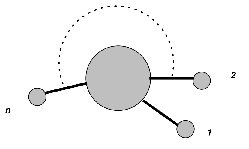
Figure 1: A general diagram consisting on $n$ 1-vertices and 1 $n$-vertex.

Its value is

$$\int^{\prime}_{q_{1}}\cdots\int^{\prime}_{q_{n}}{\tilde{S}}^{(n)}_{q_{1},\ldots,q_{n}}\prod_{i=1}^{n}\frac{{\tilde{S}}^{\prime}_{q_{i}}}{v(q_{i})}.$$ (12)

We perform the $q_{i}$-integrals in pairs, using Lemma 2 to extract the leading dependences in $\tau$. At the end, we obtain, in agreement with Lemma 3, that it is ${\cal O}(\tau^{n/2})$ for $n$ even or else ${\cal O}(\tau^{(n+1)/2})$ for $n$ odd, with the final aid of Lemma 1. (Recall the delta function hidden in Eq. 5).

Furthermore, let us assume that Lemma 3 is true for all diagrams with $K$ vertices other than 1-leg ones. Let us now prove that it is also true for diagrams with $K+1$ such vertices. To this end, note that a generic tree diagram ${\cal G}$ with $K+1$ more-than-one-leg vertices contains at least one $n$-vertex (for some $n\not=1$) with all but one leg connected to 1-vertices.

If the selected vertex is a n-vertex, with $n$ odd, perform all integrals associated with its legs but the one that connects it to the rest of the diagram. Performing the integrals in pairs, and using Lemma 2, it brings about a contribution ${\cal O}(\tau^{(n-1)/2})$. It remains a diagram $\cal G^{\prime}$ with $K$ more-than-one-leg vertices, where the former selected vertex enters now as an additional 1-vertex (with $S^{\prime}_{q}$ replaced by some other function). See Fig. 2.

If $n$ is even, then integrate over all its legs connected to 1-vertices but one. This is, using Lemma 2 again, ${\cal O}(\tau^{(n-2)/2})$. There is left over a 2-vertex connected both to the remaining sub-diagram and to a 1-vertex. It can easily be seen that it is of the same order in $\tau$ as one with the 1-vertex connected directly to the sub-diagram, without the 2-vertex. See again Fig. 2.

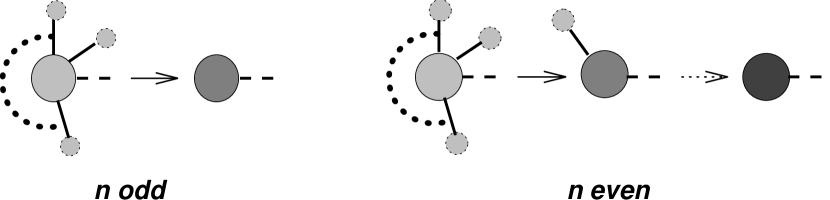
Figure 2: A vertex with $n$ integrated legs, as explained in the proof of Lemma 3. we have to distinguish between the $n$ odd and the $n$ even case.

Therefore,

$$D({\cal G})=D({\cal G^{\prime}})+\left[\frac{n-2}{2}\right]$$ (13)

and, by the induction hypothesis,

$$D({\cal G^{\prime}})=\frac{1}{2}\sum_{i}I_{2i-1}^{\cal G^{\prime}}=\left\{\begin{array}[]{lc}\frac{1}{2}I_{1}^{\cal G^{\prime}}+\frac{1}{2}\displaystyle{\sum_{i>1}}I_{2i-1}^{\cal G}&n\mbox{ even}\\ \frac{1}{2}I_{1}^{\cal G^{\prime}}+\frac{1}{2}\displaystyle{\sum_{i>1,i\not=\frac{n+1}{2}}}I_{2i-1}^{\cal G}+\frac{1}{2}I_{n}^{\cal G^{\prime}}&n\mbox{ odd}\end{array}\right.$$ (14)

Taking into account that $I^{\cal G^{\prime}}_{1}=I^{\cal G}_{1}-(n-1)+1$ and $I^{\cal G^{\prime}}_{n}=I^{\cal G}_{n}-1$, a proof of Lemma 3 follows.

QED

Note that every tree diagram must necessarily be $I_{1}\geq 2$, and, from Lemma 3, it must be $I_{1}=2$ at leading order in $\tau$. Furthermore, in such case, any inclusion of a four-legs or higher vertex would imply at least one loop, and thus the only vertices allowed, apart from one-leg ones, are an arbitrary number of two-legs ones. Even more, these additional vertices, in order to be ${\cal O}(\tau)$, are (Lemma 2)

$$\int^{\prime}_{q}\tilde{S}^{\prime\prime}_{q,-q}.$$ (15)

The argument that leads to the proof of Lemma 3 has to be slightly modified for diagrams with $L$ loops. Any 1PI part contains one $q$-integral per loop, with the only restriction that of being within the shell. After performing those integrals, we end up with a contribution ${\cal O}(\tau^{L})$ times an effective tree diagram. Therefore, the correct formula is to add the number of loops to the result of Lemma 3, but with Eq. 11 computed considering any 1PI part as a tree-level vertex.

We conclude then that there cannot be diagrams with more than one loop and that one-loop diagrams must have zero external legs. Furthermore, it happens again that diagrams with more than two legs generate further loops and that two-legs ones must have the form of Eq. 15.

All those considerations show that, at leading order in $\tau$, Eq. 4 is equivalent to

$$S[\phi]=S[\phi^{(0)}]+\int^{\prime}_{q}\phi_{q}^{(1)}S^{\prime}_{q}+\frac{1}{2}\int^{\prime}_{q}\phi_{q}^{(1)}\phi_{-q}^{(1)}S^{\prime\prime}_{q,-q}.$$ (16)

The path integral, Eq. 3, is now Gaussian with the result

$$S_{\tau}[\phi^{(0)}]=S[\phi^{(0)}]-\frac{1}{2}\int^{\prime}_{q}S^{\prime}_{q}S^{\prime}_{-q}\left(S^{\prime\prime}_{q,-q}\right)^{-1}+\frac{1}{2}\int^{\prime}_{q}\ln\left(S^{\prime\prime}_{q,-q}\right)+\mbox{const},$$ (17)

where we assume that $S^{\prime\prime}_{q,-q}$ is positive definite and “const” means a possible term independent of $\phi^{(0)}$.

The other step in any RG transformation is a change of scale in all linear dimensions. This amounts to a standard dilatation transformation,

$$k\equiv e^{\tau}q,\ \ \ \phi_{k}\equiv e^{-\tau\frac{d+2-\eta}{2}}\phi^{(0)}_{q},$$ (18)

which gives,

$$S[\phi^{(0)}] = \sum_{m}\int_{k_{1},\ldots,k_{m}}e^{-\tau md}v_{m}(e^{-\tau}k_{1},\ldots,e^{-\tau}k_{m})$$

$$\mbox{}\times\phi_{k_{1}}\ldots\phi_{k_{m}}e^{\tau m\frac{d+2-\eta}{2}}\delta_{k_{1}+\ldots+k_{m}}e^{\tau d}$$

$$= S[\phi]+\tau\left(dS-\frac{d-2+\eta}{2}\int_{k}\phi_{k}\frac{\delta S}{\delta\phi_{k}}-\int_{k}\phi_{k}k\cdot\frac{\partial^{\prime}}{\partial k}\frac{\delta S}{\delta\phi_{k}}\right)+{\cal O}(\tau^{2}),$$

where the prime in the last partial derivative merely indicates that it does not affect delta functions.

Therefore, Wegner-Houghton equation is

$$\dot{S}\equiv\frac{\partial S}{\partial t}=\lim_{\tau\rightarrow 0}\frac{S_{\tau}[\phi]-S[\phi]}{\tau}$$

$$=\lim_{\tau\rightarrow 0}\frac{1}{2\tau}\left[\int^{\prime}_{k}\ln(S_{-k,k}^{\prime\prime})-\int^{\prime}_{k}S_{-k}^{\prime}S_{k}^{\prime}\left(S_{-k,k}^{\prime\prime}\right)^{-1}\right]$$

$$\mbox{}+dS+\frac{2-d-\eta}{2}\int_{k}\phi_{k}\frac{\delta S}{\delta\phi_{k}}-\int_{k}\phi_{k}k\cdot\frac{\partial^{\prime}}{\partial k}\frac{\delta S}{\delta\phi_{k}}+\mbox{const}.$$

To deal with the $N$ arbitrary case, we define the partition function as

$$Z[J^{i}]=\int{\cal D}\phi e^{-NS[\phi^{i}/\sqrt{N}]+\int J^{i}\phi^{i}},$$ (21)

so that couplings are all finite at $N\rightarrow\infty$. The derivation is completely analogous and the ERG equation reads

$$\dot{S} = \lim_{\tau\rightarrow 0}\frac{1}{2\tau}\left[\frac{1}{N}\int^{\prime}_{k}\mbox{tr}\ln(S_{-k,k}^{j,i})-\int^{\prime}_{k}S_{-k}^{j}S_{k}^{i}\left(S_{-k,k}^{j,i}\right)^{-1}\right]$$

$$\mbox{}+dS+\frac{2-d-\eta}{2}\int_{k}\phi_{k}^{i}\frac{\delta S}{\delta\phi_{k}^{i}}-\int_{k}\phi_{k}^{i}k\cdot\frac{\partial^{\prime}}{\partial k}\frac{\delta S}{\delta\phi_{k}^{i}}+\mbox{const},$$

where the trace is over flavour indices and

$$S^{i_{1},\ldots,i_{n}}_{q_{1},\ldots,q_{n}}\equiv\left.\frac{\delta^{n}S}{\delta\phi_{q_{1}}^{i_{1}}\ldots\delta\phi_{q_{n}}^{i_{n}}}\right|_{\phi^{(1)}=0}.$$ (23)

3 Projection

The Local Potential Approximation (LPA) amounts to projecting the full action into a fixed kinetic term plus a general potential involving only the zero modes,

$$S=\frac{1}{2}\int_{k}k^{2}\phi_{k}\phi_{-k}+V(y)\delta_{0},$$ (24)

where $y\equiv\phi^{i}_{0}\phi^{i}_{0}$. The LPA is, thus, just the first term in an expansion in powers of momenta [8].

To project over constant fields, we define the operator ${\cal P}(x^{i})$ [7] which, acting on an arbitrary functional $G$, is

$${\cal P}(x^{i})G=\left.\exp\left(x^{i}\frac{\delta}{\delta\phi^{i}_{0}}\right)G\right|_{\phi_{k}=0}.$$ (25)

The projection of the third term in the second line of Eq. 2 gives zero because of the explicit factor of $k$ there. The first two terms in that line are simply

$$dV(y)\delta_{0}+\frac{2-d-\eta}{2}x^{i}\frac{\partial V(y)}{\partial x^{i}}\delta_{0}=[dV(y)+(2-d-\eta)yV^{\prime}(y)]\delta_{0},$$ (26)

with $x^{i}x^{i}\equiv y$. The second term of the right hand side of Eq. 2 can be seen to cancel whereas the first one is

$$\lim_{\tau\rightarrow 0}\frac{1}{2N\tau}\int_{k}^{\prime}\mbox{tr}\ln\left({\cal P}(x)S_{k,-k}^{i,j}\right).$$ (27)

The LPA amounts to

$${\cal P}(x)S_{k,-k}^{i,j}\longrightarrow\left(\delta^{ij}k^{2}+\frac{\partial^{2}V}{{\partial x^{i}}{\partial x^{j}}}\right)\delta_{0}.$$ (28)

Eq. 27 becomes, thus,

$$\frac{A_{d}}{2}\mbox{tr}\ln\left(\delta^{ij}+\frac{\partial^{2}V(y)}{\partial x^{i}\partial x^{i}}\right)+\mbox{const}$$ (29)

$$=\frac{A_{d}}{2}\left[\mbox{tr}\ln(1+u)+\mbox{tr}\ln\left(\delta^{ij}+2x^{i}x^{j}\frac{u^{\prime}}{1+u}\right)\right]+\mbox{const}$$

$$=\frac{A_{d}}{2}\left[(N-1)\ln(1+u)+\ln(1+u+2yu^{\prime})\right]+\mbox{const},$$

with $u(y)\equiv 2V^{\prime}(y)$,

$$A_{d}\equiv\frac{2\pi^{d/2}/\Gamma(d/2)}{(2\pi)^{d}}$$ (30)

and $\Gamma(z)$ the Euler Gamma function.

The equation is further simplified if we perform one more derivative with respect to $y$,

$$\delta_{0}\dot{u}=\frac{A_{d}}{N}\left[\frac{3u^{\prime}+2yu^{\prime\prime}}{1+u+2yu^{\prime}}+(N-1)\frac{u^{\prime}}{1+u}\right]+\delta_{0}[(2-\eta)u+(2-d-\eta)yu^{\prime}].$$ (31)

If, instead, the projection is over the kinetic term and its normalization kept fixed under the RG flow,

$$0=-p^{2}+\frac{1}{2}dp^{2}+\frac{1}{2}(2-d-\eta)p^{2},$$ (32)

it follows $\eta=0$.

Moreover, the delta function in Eq. 31 just reflects the difficulties of selecting one mode out of a continuum set. This problem is not present at finite volume, where the zero mode is neatly separated. In such a case the delta function $\delta_{0}$ is just a coefficient proportional to the inverse number of modes. One can then rescale $y\rightarrow y/\delta_{0}$ and Eq. 31 becomes

$$\dot{u}=\frac{A_{d}}{N}\left[\frac{3u^{\prime}+2yu^{\prime\prime}}{1+u+2yu^{\prime}}+(N-1)\frac{u^{\prime}}{1+u}\right]+2u+(2-d)yu^{\prime}.$$ (33)

Note that, along the same lines, one may absorb $A_{d}$.

On projecting, we made just one approximation, that of Eq. 28. Before closing the section, we briefly analyze how, in the $N\rightarrow\infty$ limit, this approximation becomes exact. Eq. 28 amounts to,

$$v_{2}(k) \rightarrow \frac{1}{2}k^{2}+v_{2}(0)$$

$$v_{m}(k,-k,0,\ldots,0) \rightarrow v_{m}(0,\ldots,0)\ \ \ m>2.$$ (34)

Hence, it becomes exact when couplings do not depend on $k$ (except for $v_{2}$ that has a $k^{2}$ term). If one expands Eq. 2 in powers of momenta, one realizes that an hypothesis of such a kind does not hold for $N$ finite, but there are some chances at $N=\infty$.

To proceed, it is necessary to rewrite Eq. 2 introducing $O(N)$ invariants,

$$\Phi_{k_{1},k_{2}}=\phi_{k_{1}}^{i}\phi_{k_{2}}^{i}.$$ (35)

Then, Eq. 2 at $N=\infty$ becomes closed for the invariants of the form $\Phi_{k_{1},k_{2}}=\delta_{k_{1}+k_{2}}\Phi_{k_{1}}$,

$$\dot{\hat{S}}=\lim_{\tau\rightarrow 0}\frac{1}{2\tau}\int_{k}^{\prime}\ln(2\frac{\delta\hat{S}}{\delta\Phi_{k}})+d\hat{S}+(2-d)\int_{k}\Phi_{k}\frac{\delta\hat{S}}{\delta\Phi_{k}}-\int_{k}\Phi_{k}k\cdot\frac{\partial^{\prime}}{\partial k}\frac{\delta\hat{S}}{\delta\Phi_{k}}+\mbox{const},$$ (36)

with $\hat{S}$ is the piece of $S$ that contains only the invariants $\Phi_{k}$ (called diagonal piece in Ref. [1]), and we set $\eta=0$ which is a general result on the $N\rightarrow\infty$ limit.

An inspection of how couplings of the diagonal piece at $k=0$ are affected by those with increasing powers of $k$ suggest that, if all couplings at a certain power of $k$ are set to zero, all the rest but the ones at $k=0$ can be simultaneously set to zero, so it should not come as a surprise that an ansatz like

$$S[\phi]=\frac{1}{2}\int_{k}k^{2}\Phi_{k}+V(\varphi^{2}),$$ (37)

with $\varphi^{2}=\int_{k}\Phi_{k}$, holds.

Indeed, Eq. 36 leads to a closed equation for $V(\varphi^{2})$,

$$\dot{V}=A_{d}\ln\left(1+V^{\prime}(\varphi^{2})\right)+dV(\varphi^{2})+(2-d)\varphi^{2}V^{\prime}(\varphi^{2})+\mbox{const},$$ (38)

which turns out to be the same as the large $N$ limit of Eq. 33. This is the result we were after. The LPA in the large $N$ limit is not only solvable as we will see in Section 6, but also exact. If our initial potential has couplings that do not depend on $k$, the exact evolution for those is governed by Eq. 38.

4 Results

Fixed Points (FPs) $u^{*}(y)$ of Eq. 33 are the analytical solutions of

$$0=\frac{A_{d}}{N}\left[\frac{3u^{\prime}+2yu^{\prime\prime}}{1+u+2yu^{\prime}}+(N-1)\frac{u^{\prime}}{1+u}\right]+2u+(2-d)yu^{\prime},$$ (39)

with $A_{d}$ some $d$-dependent constant (Eq. 30) which equals $(2\pi^{2})^{-1}$ in $d=3$. All universal quantities are independent of its precise value. Note that this is an ordinary differential equation of second order and, thus, two initial conditions are required. Nevertheless, at $y=0$ Eq. 39 is singular, since the coefficient of its highest derivative vanishes, and we must supply the analyticity condition

$$\left.u^{*}\right.^{\prime}(0)=-\frac{2N}{A_{d}(N+2)}u^{*}_{0}(1+u^{*}_{0}),\ \ \ u^{*}_{0}\equiv u^{*}(0),$$ (40)

which reduces the possible solutions to a one parameter set.

A careful study shows, however, that for any initial value $u^{*}_{0}\leq-1$ the solution remains negative for any $y$, resulting in an unbounded potential. We, thus, end up with $u^{*}_{0}>-1$ as only possible values. Furthermore, both analytical and numerical considerations show that solutions of Eq. 39 end up with a singularity

$$u(y)\begin{array}[t]{c}\sim\\ \scriptstyle y\nearrow y_{s}\end{array}\frac{A_{d}}{N(d-2)y_{s}}\ln(y_{s}-y)$$ (41)

for all but a finite number of $u^{*}_{0}$. In Fig. 3 we plot the singular point $y_{s}$ as a function of the initial condition $u^{*}_{0}$ for different values of $N$ at $d=3$.

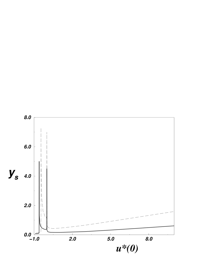
Figure 3: Point $y_{s}$ where the singularity is encountered as a function of the FP initial condition $u^{*}(0)$, for $N=1$ (dashed line) and $N=4$ (solid line), in $d=3$.

For $d<4$ only two initial values are allowed, one corresponding to the Gaussian Fixed Point (GFP) and another one to the Heisenberg Fixed Point (HFP). We study each in turn.

The GFP is

$$u^{*}(y)=0.$$ (42)

Its eigenoperators are solutions of the linearized version of Eq. 39 around $u=0$,

$$\lambda g=\frac{A_{d}}{N}[3g^{\prime}+2yg^{\prime\prime}+(N-1)g^{\prime}]+(2-d)yg^{\prime}+2g,$$ (43)

with $g(y)$ the derivative of the scaling operator and $\lambda$ its eigenvalue. For the sake of convenience, we define

$$z\equiv\frac{(d-2)Ny}{2A_{d}}$$ (44)

to obtain

$$zg^{\prime\prime}(z)+(1+\frac{N}{2}-z)g^{\prime}(z)+\frac{2-\lambda}{d-2}g(z)=0,$$ (45)

which is the generalized Laguerre equation. Polynomial solutions select $\lambda$ to be

$$\lambda=2-n(d-2)$$ (46)

with $n$ a non-negative integer, and, in such a case,

$$g(y)=L_{n}^{(N/2)}({\scriptstyle\frac{N(d-2)}{2A_{d}}}y)$$ (47)

with $L_{n}^{(N/2)}(z)$ the generalized Laguerre polynomial [9]. Critical exponents are the Gaussian ones, which allow to define massive interacting QFTs in the vicinity of this FP.

The special case of $N=1$ was previously studied in Ref. [7] in terms of the variable $x\equiv\sqrt{y}$. The solutions are the Hermite polynomials of odd degree, $H_{2n+1}(\sqrt{z})$. Indeed [9],

$$L_{n}^{(1/2)}(z)=\frac{(-1)^{n}}{n!2^{2n+1}\sqrt{z}}H_{2n+1}(\sqrt{z}).$$ (48)

On the other hand, for $N\rightarrow\infty$ the eigenvectors simplify to

$$g(y)=\left(-\frac{(d-2)N}{2A_{d}}\right)\frac{1}{n!}\left(y-\frac{A_{d}}{d-2}\right)^{n}+{\cal O}(1),$$ (49)

a result which will be derived independently in Section 6. A direct diagrammatic computation of the above results is left to Appendix A.

The HFP has to be studied numerically. From the asymptotic behaviour of Eq. 39, it is, for $y\rightarrow\infty$,

$$u(y) \sim y^{\frac{2}{d-2}}\left[B-\frac{2A_{d}}{d(d-2)}y^{-\frac{d}{d-2}}\right.$$

$$\left.\mbox{}+\frac{2A_{d}}{(d^{2}-4)}\left(1-\frac{4}{(d+2)N}\right)y^{-\frac{d+2}{d-2}}\right],$$

with $B$ an a priori unknown numerical constant. Imposing this dependency for large enough values of $y$, together with the consistency condition at $y=0$, selects the true FP out of the whole bunch of non-analytical solutions.

Recall, however, that Eq. 39 is singular at the origin. This makes it difficult to numerically integrate the equation from large $y$ towards the origin, although it is quite easy to integrate it from the origin. We circumvent this difficulty by shooting to a fitting point [10]. That is, we integrate forward to some point $y_{0}$ from a tiny value of $y$, satisfying the condition in Eq. 40. Which tiny value to take is immaterial as long as one checks it is less than the allowed errors. At $y_{0}$ we compare it with the backward integration from a large value where the asymptotic condition is imposed. In this way, the constants $u^{*}_{0}$ and $B$ from Eqs. 40, 4 are fixed. The precise value of $y_{0}$, of course, does not matter, but we found it efficient to take values close to $\sim 0.05$, where the potential is known to have a minimum in the exact solution at $N\rightarrow\infty$. Plots for some values of $N$ at $d=3$ are shown in Fig. 4, where they are compared with the corresponding large $N$ solution.

Figure 4: Solutions corresponding to the Heisenberg Fixed Point in $d=3$. The long-dashed line corresponds to $N=1$, the dashed one to $N=4$, the dotted one to $N=100$ and the solid one to $N=\infty$.

Linearizing Eq. 39 around the HFP, its eigenvectors are found to fulfil

$$\lambda g = \frac{A_{d}}{N}\left[\frac{3g^{\prime}+2yg^{\prime\prime}}{1+u^{*}+2y\left.u^{*}\right.^{\prime}}-\frac{(3\left.u^{*}\right.^{\prime}+2y\left.u^{*}\right.^{\prime\prime})(g+2yg^{\prime})}{(1+u^{*}+2y\left.u^{*}\right.^{\prime})^{2}}\right.$$ (51)

$$\left.\mbox{}+(N-1)\frac{g^{\prime}}{1+u^{*}}-(N-1)\frac{\left.u^{*}\right.^{\prime}g}{(1+u^{*})^{2}}\right]+(2-d)yg^{\prime}+2g,$$

which can be solved using similar techniques. In general, solutions will grow exponentially,

$$g(y)\sim\exp\left(\frac{d^{2}-4}{2dA_{d}}NBy^{d/(d-2)}\right),$$ (52)

whereas for special values of $\lambda$ they are much smoother,

$$g(y)\sim y^{\frac{2-\lambda}{d-2}}\left\{1+\frac{\lambda A_{d}}{d(d-2)B}\left[1-\frac{2\lambda}{N(d+2)}\right]y^{-\frac{d}{d-2}}\right.$$

$$\left.\mbox{}-\frac{(\lambda+2)A_{d}}{(d^{2}-4)B^{2}}\left[1-\frac{4(d+2)+2\lambda(d-2)}{N(d+2)^{2}}\right]y^{-\frac{d+2}{d-2}}\right\}.$$

This asymptotic behaviour, together with an arbitrary normalization of eigenvectors, leads to the quantization of $\lambda$. The results for $\nu$ and $\omega$ are summarized in Table 1, where $\nu=1/\lambda_{0}$ and $\omega=-\lambda_{1}$, $\lambda_{0}$, $\lambda_{1}$ being the first (the relevant) eigenvalue and the second (the first irrelevant) one, respectively.

$N$ $\nu$ $\omega$ $N$ $\nu$ $\omega$ $N$ $\nu$ $\omega$ 0 0.6066 0.5432 7 0.9224 0.8876 50 0.9895 0.9861 1 0.6895 0.5952 8 0.9323 0.9028 60 0.9913 0.9884 2 0.7678 0.6732 9 0.9401 0.9145 70 0.9925 0.9901 3 0.8259 0.7458 10 0.9462 0.9238 80 0.9935 0.9941 4 0.8648 0.8007 20 0.9736 0.9639 90 0.9942 0.9924 5 0.8910 0.8396 30 0.9825 0.9764 100 0.9948 0.9931 6 0.9092 0.8673 40 0.9869 0.9825 1000 0.9995 0.9994

Table 1: The critical exponents $\nu$ and $\omega$ for different values of $N$ and $d=3$. All digits are significant. The $N\rightarrow\infty$ result is $\nu=\omega=1$.

With nearly the same ease next irrelevant operators can also be studied. In Table 2 we present our results.

$N$ $\lambda_{2}$ $\lambda_{3}$ $N$ $\lambda_{2}$ $N$ $\lambda_{2}$ $N$ $\lambda_{2}$ 1 -2.8384 -5.1842 5 -2.8873 10 -2.9426 60 -2.9917 2 -2.8348 -5.1100 6 -2.9036 20 -2.9731 70 -2.9928 3 -2.8482 -5.0582 7 -2.9167 30 -2.9827 80 -2.9938 4 -2.8680 -5.0286 8 -2.9273 40 -2.9873 90 -2.9945 9 -2.9357 50 -2.9899 100 -2.9951

Table 2: The third and fourth eigenvalues, $\lambda_{2}$, $\lambda_{3}$, for different $N$s at $d=3$. All digits are significant. The $N\rightarrow\infty$ result is $\lambda_{2}=-3$, $\lambda_{3}=-5$.

The $N=1$ case was first computed in Ref. [7], with results $\nu=0.687(1)$ and $\omega=0.595(1)$, and afterwards in Ref. [11]. Our numbers are compatible with the former and coincide with the latter.

Eigenoperators are obtained as an additional bonus. As a matter of example, we plot in Fig. 5 the first eigenvector, normalized to $g(0)=1/2$, corresponding to different values of $N$ at $d=3$.

Figure 5: The first eigenoperator, normalized to $g(0)=1/2$, for $N=1$ (long-dashed line), $N=4$ (dashed line), $N=100$ (dotted line), $N=\infty$ (solid line), at $d=3$.

The $N\rightarrow 0$ limit deserves a special remark, as the RG equation 33 is singular at $N=0$. Nevertheless, one may compute its eigenvalues in an indirect way. Taking values of $N$ between $0.1$ and $0.01$, one finds that they perfectly fit a straight line, with no sign at all of subleading corrections. Critical exponents reported in Table 1 are just their extrapolation to $N=0$. In Fig. 6 we plot the first eigenvalue for $0.01<N<0.1$ together with its linear extrapolation.

Figure 6: The first eigenvalue for small values of $N$ at $d=3$. The dots are the calculated numbers, the straight line is fitted to extrapolate to $N=0$.

This apparent singularity at $N=0$ is, however, due to the rescaling in Eq. 21. Had we defined the partition function without explicit factors of $N$, the $A_{d}/N$ coefficient in RG Eq. 33 would be simply $A_{d}$, allowing a direct analysis of the $N\leq 0$ values. We just decided to stick to our normalization.

5 Comparison with other equations

In this section we comment on other ERG equations and compare with known results.

Apart from the Wegner-Houghton equation studied above, one of the oldest ERG equations appeared in Ref. [6]. It was further modified by Polchinski [2] to put it in the form we now use. The regulator is chosen in such a way that every propagator is multiplied by a function $K(p^{2})$ which is analytic everywhere in the finite complex plane, vanishes faster than any polynomial for large real values of its argument and it is standardly normalized to $K(0)=1$ [12]. The evolution of the action takes the form

$$\dot{S} = \frac{\delta S}{\delta\phi}\cdot K^{\prime}\cdot\frac{\delta S}{\delta\phi}-\frac{1}{N}\,\mbox{tr}\left(K^{\prime}\cdot\frac{\delta^{2}S}{\delta\phi\delta\phi}\cdot\right)-2\phi\cdot p^{2}K^{-1}K^{\prime}\frac{\delta S}{\delta\phi}$$ (54)

$$\mbox{}+dS+\frac{2-d-\eta(t)}{2}\,\phi\cdot\frac{\delta S}{\delta\phi}-\phi\cdot\left(p\cdot\frac{\partial^{\prime}}{\partial p}\right)\frac{\delta S}{\delta\phi}+\mbox{const},$$

where a dot means both summation over discrete variables and integration over continuous ones. As the non-linearities are limited to quadratic terms, the projected equation presents a nice form quite amenable for numerical analysis,

$$\dot{u}=\frac{2y}{N}u^{\prime\prime}+\left(1+\frac{2}{N}+(2-d)y-2yu\right)u^{\prime}+(2-u)u,$$ (55)

where a convenient rescaling of the potential and the field variable $y$ has been made. It has been previously studied for $N=1$, using the variable $x\equiv\sqrt{2y}$, in Ref. [13].

The GFP is also $u=0$, with its eigenoperators satisfying Eq. 45 after the rescaling $z\equiv\frac{N}{2}(d-2)y$. The solution $u=2$ corresponds to the Trivial Fixed Point, also known as High Temperature Fixed Point.

The analysis of the HFP is analogous to the Wegner-Houghton one. There are singular solutions which behave

$$u\sim\frac{2}{N}\frac{1}{y_{s}-y},$$ (56)

whereas the true FP must fulfil the conditions

$$\left.u^{*}\right.^{\prime}(0) = \frac{N}{N+2}u^{*}(0)(u^{*}(0)-2),$$

$$u^{*}(y) \begin{array}[t]{c}\sim\\ \scriptstyle y\rightarrow\infty\end{array} 2-By^{-\frac{2}{2+d}}$$ (59)

with $B$ a non-vanishing constant. Again we can shoot to a fitting point to obtain the FP. Eigenvalues $\lambda$ are obtained from the linearized form of Eq. 55 imposing the eigenvectors to be $g\sim y^{-(\lambda+2)/(d+2)}$ for $y\rightarrow\infty$. Some of them are shown in Tables 3, 4. We leave to Appendix B the study of its large $N$ limit.

Another quite used equation is based on the evolution of an infrared-regulated one-particle-irreducible effective action [3],

$$\frac{\partial}{\partial\Lambda}\Gamma[\varphi]=-\frac{1}{2}\mbox{tr}\left[K^{-1}\frac{\partial K}{\partial\Lambda}\cdot\left(1+K\cdot\frac{\delta^{2}\Gamma}{\delta\varphi\delta\varphi}\right)^{-1}\right],$$ (60)

where $K$ is some regulating function and $\Gamma[\varphi]$ is the effective action minus the kinetic term $\frac{1}{2}\varphi\cdot K^{-1}\cdot\varphi$. It presents some attractive features: in the limit where the IR cutoff vanishes (which corresponds to the continuum limit) it is directly observable, as it is the equation of state of the system. Moreover, it presents a natural expansion which can be directly mapped to the usual loop expansion of perturbation theory [14]. Various regulators have been used in connection with this equation. If a sharp momentum cutoff is chosen, its LPA coincides with that of Wegner-Houghton’s. On the other hand, it has been extensively worked out using the special polynomial cutoff introduced in Ref. [15], which has the advantage of preserving some symmetries of the exact equation through the derivative expansion. This equation is much harder to numerically analyze than the above two ones. We do not discuss it further, but only quote the results (Tables 3, 4) and refer the reader to the original literature [15, 16].

To assess the systematic errors involved in such calculations would require to compute corrections to the LPA. Instead, we compare our results with some derived from other techniques.

There are accurate determinations for $\nu$ from a variety of methods such as $\varepsilon$ expansion [17], Monte Carlo Renormalization Group [18, 19], Monte Carlo simulations [20, 21] and Strong-Coupling series [22]. Unfortunately, estimates for $\omega$ are not so precise. A comparison of our results from Wegner-Houghton and Polchinski equations with those from the IR-cutoff effective action and other existing estimates are shown in Tables 3, 4.

$N$ (1) (2) (3) (4) 0 0.6066 0.5880(15) [17] 1 0.6895 0.6496 0.6604 [15] 0.624(1)(2) [18] 2 0.7678 0.7082 0.73 [16] 0.6721(13) [20] 3 0.8259 0.7611 0.78 [16] 0.7128(14) [20] 4 0.8648 0.8043 0.824 [16] 0.7525(15) [20]

Table 3: Critical exponent $\nu$, at $d=3$, for different values of $N$, using different RG equations (all digits are significant): (1) Wegner-Houghton, (2) Polchinski, (3) effective action; together with accurate determinations (4).

$N$ (1) (2) (3) (4) 0 0.5432 0.80(4) [17] 1 0.5952 0.6557 0.6285 [15] 0.85(5) [18] 2 0.6732 0.6712 0.66 [16] 0.780(25) [17] 3 0.7458 0.6998 0.71 [16] 0.800(25) [17] 4 0.8007 0.7338 0.75 [16] ?

Table 4: Critical exponent $\omega$, at $d=3$, for different values of $N$, using different RG equations (all digits are significant): (1) Wegner-Houghton, (2) Polchinski, (3) effective action; together with existing estimates (4).

Critical indices from Wegner-Houghton equation are $10-15\%$ off for $N<10$, except at $N=0$, which is quite accurate ($\sim 3\%$). In the interval $10<N<100$, they are off by a few per cent, and for $N>100$, the errors are less than one per mile. Other ERG perform slightly better, specially Polchinski’s equation in which critical indices are a few per cent off at most. This should not come as a surprise, since in spite of its conceptual clarity, the sharp momentum cut-off leads to bad locality properties of the renormalized actions, being then very much sensitive to truncations. In order for the projected ERG equation to deliver more precise outcomes, one should find RG blockings with the property that renormalized actions are as much local as possible, as it is achieved in the lattice regularization with blockings in real space [23].

6 $N\rightarrow\infty$

Wegner and Houghton [1] already studied the limit $N\rightarrow\infty$ of their equation, encountering both the GFP and the HFP. They also briefly mentioned the possibility of further FPs. Our aim is to discuss in certain detail those not previously studied and present a general framework to deal with this kind of large $N$ equations. An application of these methods for the Polchinski equation is given in Appendix B.

The projected RG equation becomes first order in the $N\rightarrow\infty$ limit,

$$\dot{u}=A_{d}\frac{u^{\prime}}{1+u}+(2-d)yu^{\prime}+2u,$$ (61)

which is easily solved for $2<d<4$ once we invert $u$ and consider $y(u,t)$,

$$\dot{y}=-2uy^{\prime}-(2-d)y-\frac{A_{d}}{1+u}.$$ (62)

The prime now stands for derivative with respect to $u$. Its general solution is

$$y(u,t)=e^{(d-2)t}h(e^{-2t}u)+f(u),$$ (63)

with an arbitrary function $h(z)$ and

$$f(u)=A_{d}\left(\frac{1}{d-2}+u\int_{0}^{1}dz\frac{z^{3-d}}{1+uz^{2}}\right),$$ (64)

which is analytic for $u>-1$. Although derived differently, this is the form of the ERG equation used in Refs. [24, 25] for $d=3$.

Returning to Eq. 61, FPs verify

$$u^{\prime}=\frac{2u}{(d-2)y-\frac{A_{d}}{1+u}},$$ (65)

which can be singular when the denominator of the rhs vanishes. But, if this is the case, then analyticity of the FP would imply $u=0$, and, therefore, these would-be singular points reduce to a unique one,

$${\tilde{y}}\equiv\frac{A_{d}}{d-2},\ \ \ u(\tilde{y})=0.$$ (66)

Furthermore, we can Taylor expand the FP around $\tilde{y}$,

$$u(y)=a(y-\tilde{y})+\sum_{k=2}^{\infty}a_{k}(y-\tilde{y})^{k},$$ (67)

an expansion that will be used throughout.

Eigenoperators are

$$g_{\lambda}(y)=\exp\int_{0}^{y}dz\,t_{\lambda}(z),$$ (68)

with

$$t_{\lambda}(y)=\left[\frac{A_{d}u^{\prime}}{(1+u)^{2}}+\lambda-2\right]\left[\frac{A_{d}}{1+u}-(d-2)y\right]^{-1}.$$ (69)

Eq. 67 fixes the only singularity of $t_{\lambda}(y)$ to be a pole at $\tilde{y}$, with residue

$$\frac{1}{1+a\tilde{y}}\left(\frac{\lambda-2}{2-d}-a\tilde{y}\right).$$ (70)

For eigenoperators to be single-valued, the residue must be a nonnegative integer $n$, which fixes

$$\lambda_{n}=2+(2-d)[a\tilde{y}+n(1+a\tilde{y})].$$ (71)

Note how critical properties of the system are completely determined by the behaviour of the FP around this special point $\tilde{y}$.

After those general considerations let us study the different FPs in turn. The easiest one is the GFP, which corresponds to

$$u(y)=0\Rightarrow a=0\Rightarrow\lambda_{n}=2-n(d-2)$$ (72)

and, from Eq. 68,

$$g(y)=(y-\tilde{y})^{n},$$ (73)

a result previously obtained in Eq. 49.

The HFP corresponds to $h(z)=0$ in Eq. 63,

$$y(u)=f(u)=A_{d}\left(\frac{1}{d-2}+u\int_{0}^{1}dz\frac{z^{3-d}}{1+uz^{2}}\right).$$ (74)

In this case, $a=\frac{4-d}{A_{d}}$. Hence,

$$\lambda_{n}=d-2-2n,$$ (75)

which are the critical exponents of the spherical model. Eigenvectors are obtained plugging Eq. 74 in Eq. 68. Note that in the limit $d\rightarrow 4$, the HFP merges with the GFP, as can be seen both from Eqs. 74 and 75.

However, contrary to the finite $N$ case, there are more FP. They correspond to $e^{(d-2)t}h(e^{-2t}u)$ becoming t-independent,

$$y(u)-\tilde{y}=Cu^{\frac{d-2}{2}}+A_{d}u\int^{1}_{0}dz\frac{z^{3-d}}{1+uz^{2}},$$ (76)

with $C$ a, so far, arbitrary constant. The behaviour around $\tilde{y}$,

$$u(y)=\left(\frac{y-\tilde{y}}{C}\right)^{\frac{2}{d-2}}+{\cal O}\left((y-\tilde{y})^{\frac{4}{d-2}}\right),$$ (77)

defines for $2/(d-2)=n$, $n=2,3,\ldots$ a line of FP labelled by the parameter $C$. Since $a=0$, critical indices coincide with those of the GFP, for all allowed values of $C$.

Before getting into a detailed analysis, let us state that, for any allowed $C$, these FPs are reached by Eq. 63, at $t\rightarrow\infty$, from an initial potential

$$V(y)=\frac{C}{2(n+1)}\left(\frac{y-nA_{d}/2}{C}\right)^{n+1},$$ (78)

which shows that those FPs encode the large distance properties of local actions. Note that $C=+\infty$ corresponds to the GFP.

To proceed further, we should distinguish between $n$ odd and $n$ even. The FP in the $n$ odd case is

$$y=Cu^{\frac{1}{n}}+A_{d}\left(\frac{n}{2}+u\int_{0}^{1}dt\frac{t^{1-2/n}}{1+ut^{2}}\right).$$ (79)

The admissible values of $C$ are $0<C\leq\infty$. Although the HFP corresponds to $C=0$, it does not belong to this line of FPs. This is not so surprising in view of Eq. 78: critical properties are not continuous in $C$ at $C=0$. Note, however, that these singularities have nothing to do with RG transformations: $C$ labels different initial conditions for the RG transformations, but once one $C$ is chosen, it is not changed along the flow.

The FP in the $n$ even case comes from matching the two branches of $y(u)$ at $\tilde{y}$,

$$y=\left\{\begin{array}[]{lc}-Cu^{\frac{1}{n}}+f(u)&0\leq y\leq\tilde{y}\\ +Cu^{\frac{1}{n}}+f(u)&y\geq\tilde{y}\end{array}\right.$$ (80)

Now the line of FPs extend from $C=+\infty$ up to the end point

$$C=\frac{A_{d}\pi}{2\sin\frac{\pi}{n}},$$ (81)

which appears as the existence condition of the FP at $y=0$.

The case $C=\frac{A_{d}\pi}{2\sin\frac{\pi}{n}}$ deserves further considerations because the FP is not analytical at $y=0$. It behaves like $u(y)=\frac{nA_{d}}{2(n+1)}\frac{1}{y}+{\cal O}(1)$, and its eigenvectors like,

$$g_{k}(y)\sim y^{-\frac{(n+1)(n+1-k)}{n(n-1)}}.$$ (82)

The case $n=2$ ($d=3$) were previously studied in Ref. [25] and these features were identified as the RG structures which make the existence of the BMB phenomenon [26] possible. That is, the possibility that at $C=\frac{A_{3}\pi}{2\sin\frac{\pi}{2}}$, the FP acts as an ultraviolet stable one, allowing to define a new continuum limit other than the Gaussian and Heisenberg FPs. In fact one that has mass generation and spontaneous symmetry breaking of scale invariance accompanied with the appearance of a dilaton. What we now see, is that all RG properties that make this phenomenon to appear at $d=3$, are present for all the rest of $n$ even values, hence a similar scenario is likely to take place. To elucidate these issues would require a further analysis of the effective potential at the vicinity of this peculiar FP. This is, however, beyond the scope of this paper.

The preceding considerations have shown the existence of a line of FPs starting at the GFP and including it. This scenario is only feasible provided that the GFP contains marginal non-redundant operators. This restricts the dimensions of space (space-time) to be

$$d=2+\frac{2}{n},\ \ \ n=2,3,\ldots$$ (83)

which gives a nice physical interpretation of the dimensions previously derived from analyticity considerations. Thus, in the large $N$ limit, the marginal operator becomes completely marginal and a line of inequivalent FP appears, though they have the critical exponents of the GFP. This might be a general feature of this limit.

Before closing this section we would like to remark that, although our analysis of Eq. 62 is restricted to dimensions $2<d<4$, a similar study in other dimensions is possible along the same lines. For instance, in $d=4$, Eq. 63 is substituted by

$$y(u,t)=e^{2t}h(e^{-2t}u)+\frac{u}{8\pi^{2}}t+\frac{1}{16\pi^{2}}-\frac{u}{8\pi^{2}}\int_{0}^{1}dz\,\frac{z}{1+uz^{2}},$$ (84)

which does not have any FP other than the GFP, $u=0$. On the contrary, at $d=2$,

$$y(u,t)=h(e^{-2t}u)-\frac{t}{2\pi}+\frac{1}{4\pi}\ln(1+u),$$ (85)

where a FP appears for $h(z)=-\frac{1}{4\pi}\ln(z)$. A thorough study for all $d$ would take us too far afield.

7 Conclusions

This paper presented a detailed study of Wegner-Houghton equation. We have shown that in spite of its intractable appearance, the use of the LPA makes it amenable for extracting plenty of valuable information.

The derivation of the equation has been worked out, with special care about the terms that contribute to the blocking. The projection has been derived, and explained in which sense it is exact in the $N\rightarrow\infty$ limit.

What we feel remarkable about the ERG methods within the LPA is, succinctly; (i) The qualitative features of the RG at $2<d\leq 4$ are the same as in the expected full computation; (ii) Eigenvalues and eigenvectors are obtained with ease, both relevant and irrelevant ones; (iii) Numerical results are, at this order in the derivative expansion, not as accurate as other methods, at least for low enough $N$, but those are computationally much harder; (iv) The $N\rightarrow 0$ limit is reliable within this framework.

The LPA of Polchinski equation has been also studied, and found that the accuracy is improved. This suggests that a calculation of next order in the momentum expansion may deliver quite rigorous results. Nevertheless, ambiguities appear in connection with the determination of the non-vanishing anomalous dimension, which are not present at lowest order [13]. A further study of these issues, hence, seems justified [27].

Section 6 has been devoted to the $N\rightarrow\infty$ limit. Some existing results, scattered throughout the literature, have been reviewed within a general framework, which has also been fruitful to study new FPs at critical dimensions $d=2+2/n$, as well as to deal with other RG equations. As an example, we have worked out the large $N$ limit of Polchinski equation.

The scope of the paper did not permit to consider other subjects of interest. Among those, the study of the projected RG equation 33, outside the linear approximation, useful to elucidate the topology of the RG [7, 28]; the study of the effective potential of the new FPs at $N\rightarrow\infty$, with special emphasis on the singularities that we associate to the BMB phenomenon; and a more systematic study of Polchinski equation. We hope that those issues will be tackled in a near future.

Before closing, we would like to come back to our original motivation on first-order phase transitions, singling out some of our results which have implications for them. We have explicitly shown in Section 3 that in the large $N$ limit, the LPA is exact (see Eq. 38). This equation, in the form of Eq. 63, was shown in Ref. [7] to lead to singularities of the RG whenever two competing minima exist, which is the case when first-order phase transitions take place. Those exact results point that the RG trajectories are singular and multi-valued, which is at odds with Fundamental Theorems One and Two of Refs. [4]. Nonetheless, one should keep in mind that those theorems do not rigorously apply for unbounded spins. On the other hand, the derivation of Wegner-Houghton equation of Section 2 assume positivity of the eigenvalues of $S^{\prime\prime}_{q,-q}$, at the step of Eq. 17, which, as suggested in Ref. [7], may not be the case if metastable states do exist. A further study on all those subjects is beyond the scope of this paper, but we think that they pose interesting questions on the conventional wisdom of the RG.

Appendix A The Gaussian RG Equation

In this section we work out the GFP from a direct computation of the partition function, reobtaining in quite a different way expressions already quoted in Section 4. We use diagrammatic techniques very similar to the ones in deriving the approximate recursion formula [6]. We explicitly treat the $N=1$ case, but the $N$ arbitrary situation is completely analogous.

We consider the splitting in Eq. 2,

$$\phi_{q}=\phi^{(0)}_{q}+\phi^{(1)}_{q},$$ (86)

but now $\phi^{(1)}$ accounts for modes with $\frac{1}{2}<q\leq 1$. Then, the dilatation in Eq. 18 is

$$k\equiv 2q,\ \ \ \phi_{k}=2^{-\frac{d+2}{2}}\phi^{(0)}_{q}.$$ (87)

We consider our action as the GFP and the subspace spanned by (ultra-)local operators,

$$S[\phi]={\cal I}+\frac{1}{2}\int_{q}\phi_{q}q^{2}\phi_{-q}+\sum_{l=2,4,\ldots}g^{(l)}\int d^{d}x\phi^{2l}(x),$$ (88)

where we explicitly include the identity.

The linear approximation amounts to consider $g^{(l)}$ couplings to be infinitesimal. In such a case we can compute perturbatively the flow. In Fig. 7, the three diagrams (A,B,C) generated from a quartic coupling are shown.

Figure 7: Diagrams to be considered, where solid lines mean integrated modes and dashed lines are not. A, B, C, are the contributions of the quartic vertex to the identity, the mass operator and the quartic coupling itself. D is a generic diagram with $L$ loops.

A generic diagram of a $2n$ operator with $L$ loops, like the one in Fig. 7 D, gives a contribution to the $2n-2L$ coupling

$$\frac{(2n)!c^{L}}{(2n-2L)!L!2^{L}}2^{2n-2L+d(1-n+L)},$$ (89)

where $c=\int_{\frac{1}{2}<|q|\leq 1}\frac{1}{q^{2}}$. The linear RG matrix is upper triangular, with non-vanishing matrix elements,

$$T_{l,k}=\frac{(2k)!c^{k-l}}{(2l)!(k-l)!}2^{3l-k+d(1-l)}.$$ (90)

The main result is that the eigenoperators of the linearized RG matrix are

$$O_{n}(x)=\sum_{l=0}^{n}g^{(l)}_{n}\phi^{2l}(x)=\sum_{l=0}^{n}\frac{(2n)!}{(2l)!(n-l)!}\left(\frac{c}{2(2^{2-d}-1)}\right)^{n-l}\phi^{2l}(x),$$ (91)

with eigenvalues $\Lambda_{n}\equiv 2^{\lambda_{n}}=2^{(1-n)d+2n}$. The proof is by direct substitution,

$$\sum_{k}T_{l,k}g^{(k)}_{n} = 2^{3l-n+d(1-l)}c^{(n-l)}\frac{(2n)!}{(2l)!}\sum_{k=l}^{n}\frac{(2^{2-d}-1)^{k-n}}{(n-k)!(k-l)!}$$ (92)

$$= 2^{2n+d(1-n)}\frac{(2n)!}{(2l)!(n-l)!}\left(\frac{c}{2(2^{2-d}-1)}\right)^{n-l}=\Lambda_{n}g^{(l)}_{n},$$

where the relation

$$\sum_{k=l}^{n}\frac{(n-l)!}{(k-l)!(n-k)!}a^{k}=\sum^{n-l}_{k=0}{n-l\choose k}a^{l+k}={(1+a)}^{n-l}a^{l}$$ (93)

has been used. Eq. 91 may be now rewritten as

$$O_{n}(x)=\left(\frac{A_{d}}{2(d-2)}\right)^{n}H_{2n}\left({\scriptstyle\sqrt{\frac{d-2}{2A_{d}}}}\,\phi(x)\right),$$ (94)

since $c={\displaystyle\int_{\scriptscriptstyle\frac{1}{2}<|q|\leq 1}}\frac{1}{q^{2}}=\frac{A_{d}}{d-2}(1-2^{(2-d)})$. $H_{2n}$ are the Hermite polynomials, which, after using the relation [9]

$$H_{2n}^{\prime}(x)=4nH_{2n-1}(x),$$ (95)

reduce to the result already quoted in Eq. 48.

Appendix B $N\rightarrow\infty$ with Polchinski equation

In this appendix, we sketch the results for the large $N$ limit of Polchinski equation. Our aim is twofold: on one hand to show that our techniques introduced for Wegner-Houghton equation are quite general and may be easily applied to other RG equations as well; also to prove that the annoying restriction $u>-1$ of the former equation is not an essential feature. This last fact would make interesting to repeat the large $N$ analysis of Ref. [5] for Polchinski equation.

At $N\rightarrow\infty$, Eq. 55 becomes

$$\dot{u}=[1-(d-2)y-2yu]u^{\prime}+(2-u)u.$$ (96)

Its general solution is

$$y(u,t)=\frac{e^{(d-2)t}}{(2-u)^{2}}\,h\left(\frac{ue^{-2t}}{2-u}\right)+f(u),$$ (97)

with $h(z)$ an arbitrary function and

$$f(u)=\frac{2}{d-2}\,(2-u)^{-1}+\frac{d}{d-2}\,u(2-u)^{-\frac{d+2}{2}}\int_{0}^{1}dz\left(\frac{2-uz}{z}\right)^{\frac{d-2}{2}}.$$ (98)

Note that $f(u)$ is analytic for $u<2$, unlike the Wegner-Houghton case, in which analyticity has a lower bound at $u=-1$.

For $\dot{u}=0$ the point $\tilde{y}\equiv\frac{1}{d-2}$ satisfies $u(\tilde{y})=0$. Expanding the FP solution around it, $u(y)=a(y-\tilde{y})+{\cal O}\left((y-\tilde{y})^{2}\right)$, and imposing the eigenoperators to be analytic at $\tilde{y}$, $g(y)\sim(y-\tilde{y})^{n}$, the condition for eigenvalues equivalent to Eq. 71 is

$$\lambda_{n}=2(1-\tilde{y}a)-n(d-2+2\tilde{y}a).$$ (99)

The GFP corresponds to $u=a=0$, with eigenoperators

$$g(y)=(y-\tilde{y})^{n},\ \ \ n=\frac{2-\lambda}{d-2}.$$ (100)

The HFP corresponds to $h(z)=0$, which gives $a=\frac{(d-2)(4-d)}{2}$ and $\lambda=d-2-2n$.

There is a line of FPs for $d=2+2/n$,

$$y(u)=\frac{C}{u(2-u)}\left(\frac{u}{2-u}\right)^{\frac{d}{2}}+f(u),$$ (101)

which starts at $C=+\infty$ (GFP). It ends, for $n$ odd, at $C=0$ (but without reaching the HFP) and, if $n$ is even, at $C=C_{0}\equiv\frac{\pi d}{\sin\frac{\pi}{n}}$. Precisely $C=C_{0}$, for $n$ even, is the only value where the FP is analytical at $u=2$ (it is Taylor-expandable around $y=\frac{1}{d+2}$, with $u(\frac{1}{d+2})=2$). This allows $u={\cal O}(\frac{1}{y})$ in the vicinity of $y=0$, like in the Wegner-Houghton case. These non-analyticities associated to the BMB phenomenon seem to present, therefore, some kind of universality.

References

- [1] F.J. Wegner and A. Houghton, Phys. Rev. A 8 (1973) 401
- [2] J. Polchinski, Nucl. Phys. B 231 (1984) 269
- [3] T.R. Morris, Int. J. Mod. Phys. A 9 (1994) 2411
- [4] A.C.D. van Enter, R. Fernández and A.D. Sokal, J. Statist. Phys. 72 (1993) 879
- [5] A. Hasenfratz and P. Hasenfratz, Nucl. Phys. B 295 (1988) 1
- [6] K.G. Wilson and J. Kogut, Phys. Reports 12 (1974) 75
- [7] A. Hasenfratz and P. Hasenfratz, Nucl. Phys. B 270 (1986) 687
- [8] T.R. Morris, Nucl. Phys. B 458 (1996) 477
- [9] M. Abramowitz and I.A. Stegun, ”Handbook of Mathematical Functions” (Dover, 1972)
- [10] W.H. Press, S.A. Teukolsky, W.T. Vetterling and B.P. Flannery, “Numerical Recipes, Second Edition” (Cambridge Univ. Press, 1992)
- [11] T.R. Morris, Phys. Lett. B 334 (1994) 355
- [12] R.D. Ball and R.S. Thorne, Ann. Phys. 236 (1994) 117
- [13] R.D. Ball, P.E. Haagensen, J.I. Latorre and E. Moreno, Phys. Lett. B 347 (1995) 80;
- [14] T. Pappenbrock and C. Wetterich, Z. Phys. C 65 (1995) 519
- [15] T.R. Morris, Phys. Lett. B 329 (1994) 241
- [16] T.R. Morris, “Properties of Derivative Expansion. Approximations to the Renormalization Group”, Proceedings of the Second RG Conference, Dubna, September 1996
- [17] J.C. Le Guillou and J. Zinn-Justin, Phys. Rev. B 21 (1980) 3977
- [18] C.F. Baillie, R. Gupta, K.A. Hawick and S. Pawley, Phys. Rev. B 45 (1992) 10 438
- [19] G.S. Pawley, R.H. Swendsen, D.J. Wallace and K.G. Wilson, Phys. Rev. B 29 (1984) 4030; D. Espriu and A. Travesset, Phys. Lett. B 356 (1995) 329
- [20] H.G. Ballesteros, L.A. Fernández, V. Martín Mayor and A. Muñoz Sudupe, Phys. Lett. B 387 (1996) 125
- [21] A.P. Gottlob and M. Hasenbusch, Physica A 201; (1993) 593; C. Holm and W. Janke, Phys. Lett. A 173 (1993) 8; K. Kanaya and S. Kaya, Phys. Rev. D 51 (1995) 2404
- [22] C. Domb, and J.C. Lebowitz, Phase transitions and Critical phenomena, Vol. 3, 9 (Academic Press, 1984)
- [23] T.L. Bell and K.G. Wilson, Phys. Rev. B 11 (1975) 3431
- [24] S. Ma, Phys. Lett. A 43 (1973) 479
- [25] F. David, D.A. Kessler and H. Neuberger, Phys. Rev. Lett. 53 (1984) 2071; Nucl. Phys. B 257 (1985) 695
- [26] W.A. Bardeen, M. Moshe and M. Bander, Phys. Rev. Lett. 52 (1984) 1188
- [27] J. Comellas, Barcelona preprint UB-ECM-PF 97/05 (hep-th/9705129)
- [28] C. Bagnuls and C. Bervillier, J. Phys. Studies, 1 (1997) 1
- [29] K. Aoki, K. Morikawa, W. Souma, J. Sumi and H. Terao, Prog. Theor. Phys. 95 (1996) 409 (hep-ph/9612458)
- [30] G. Eyal, M. Moshe, S. Nishigaki and J. Zinn-Justin, Nucl. Phys. B 470 (1996) 369