CERN-TH/96-365

hep-th/9612202

December, 1996

Solvable Lie Algebras
in Type IIA, Type IIB and M Theories^∗
Laura Andrianopoli¹, Riccardo D’Auria ², Sergio Ferrara²,
Pietro Fré³, Ruben Minasian² and Mario Trigiante⁴

¹ Dipartimento di Fisica Universitá di Genova, via Dodecaneso 33, I-16146 Genova
and Istituto Nazionale di Fisica Nucleare (INFN) - Sezione di Genova, Italy
² CERN, Theoretical Division, CH 1211 Geneva, Switzerland,
³ Dipartimento di Fisica Teorica, Universitá di Torino, via P. Giuria 1, I-10125 Torino,
Istituto Nazionale di Fisica Nucleare (INFN) - Sezione di Torino, Italy
⁴ International School for Advanced Studies (ISAS), via Beirut 2-4, I-34100 Trieste
and Istituto Nazionale di Fisica Nucleare (INFN) - Sezione di Trieste, Italy

Abstract

We study some applications of solvable Lie algebras in type $IIA$, type $IIB$ and $M$ theories. $RR$ and $NS$ generators find a natural geometric interpretation in this framework. Special emphasis is given to the counting of the abelian nilpotent ideals (translational symmetries of the scalar manifolds) in arbitrary $D$ dimensions. These are seen to be related, using Dynkin diagram techniques, to one-form counting in $D+1$ dimensions. A recipe for gauging isometries in this framework is also presented. In particular, we list the gauge groups both for compact and translational isometries. The former agree with some results already existing in gauged supergravity. The latter should be possibly related to the study of partial supersymmetry breaking, as suggested by a similar role played by solvable Lie algebras in $N=2$ gauged supergravity.  ^∗ Supported in part by EEC under TMR contract ERBFMRX-CT96-0045, in which L. Andrianopoli and R. D’Auria are associated to Torino University and S. Ferrara and M. Trigiante are associated to Frascati and by DOE grant DE-FG03-91ER40662.

1 Introduction

Hidden non compact symmetries of extended supergravities [1] have recently played a major role in unreaveling some non perturbative properties of string theories such as various types of dualities occurring in different dimensions and in certain regions of the moduli spaces [2].

In particular their discrete remnants have been a crucial importance to discuss, in a model independent way, some physical properties such as the spectrum of BPS states [3], [4], [5] and entropy formulas for extreme black–holes [6][7].

It is common wisdom that such U–dualities should play an important role in the understanding of other phenomena such as the mechanism for supersymmetry breaking, which may be due to some non perturbative physics [8],[9],[10].

Recently, we have analyzed some properties of U–duality symmetries in any dimensions in the context of solvable Lie algebras [11].

In string theories or M–theory compactified to lower dimensions [12], preserving $N>2$ supersymmetries, the U–duality group is generically an infinite dimensional discrete subgroup $U(\mathchoice{\hbox{\cmss Z\kern-3.99994ptZ}}{\hbox{\cmss Z\kern-3.99994ptZ}}{\lower 0.9pt\hbox{\cmsss Z\kern-2.79996ptZ}}{\lower 1.2pt\hbox{\cmsss Z\kern-2.79996ptZ}})\subset U$, where $U$ is related to the non–compact symmetries of the low energy effective supergravity theory [13].

The solvable Lie algebra $G_{S}=Solv(U/H)$ with the property $\exp[G_{S}]=U/H$, where $U/H$ is (locally) the scalar manifold of the theory, associates group generators to each scalar, so that one can speak of NS and R–R generators.

Translational symmetries of NS and/or R–R fields are associated with the maximal abelian nilpotent ideal of ${\cal A}\subset G_{S}$, with a series of implications.

The advantage of introducing such notion is twofold: besides that of associating generators with scalar fields when decomposing the U–duality group with respect to perturbative and non perturbative symmetries of string theories, such as T and S–duality in type IIA or $SL(2,{\rm I\kern-1.79993ptR})$ duality in type IIB, one may unreveal connections between different theories and have an understanding of N–S and R–R generators at the group–theoretical level, which may hold beyond a particular perturbative framework. Furthermore, the identification $U/H\sim\exp[G_{S}]$ of the scalar coset manifold with the group manifold of a normed solvable Lie algebra allows the description of the local differential geometry of $U/H$ in purely algebraic terms. Since the effective low energy supergravity lagrangian is entirely encoded in terms of this local differential geometry, this fact has obvious distinctive advantages.

In the present paper we derive a certain number of relations among solvable Lie algebras which explain some of the results obtained by some of us in a previous work.

In particular, we show that the Peccei–Quinn (translational) symmetries of $U_{D}/H_{D}$ in $D=10-r$ dimensions are classified by $U_{D+1}$, while their NS and R–R content are classified by $O(r-1,r-1)$.

For $D>3$ this content corresponds to the number of vector fields in the $D+1$ theory, at least for maximal supergravities.

An explicit expression for these generators is given and an interpretation in terms of branes is also obtained.

We also compare different decompositions of solvable Lie algebras in IIA, IIB and M–theory in toroidal compactifications which preserve maximal supersymmetry (i.e. 32 supercharges). Solvable Lie algebras in the context of compactifications preserving lower supersymmetries will be discussed elsewhere.

While in Type IIA the relevant decomposition is with respect to the S–T duality group, in IIB theory we decompose the U–duality group with respect to $SL(2,{\rm I\kern-1.79993ptR})\times GL(r,{\rm I\kern-1.79993ptR})$ and in M–theory with respect to $GL(r+1,{\rm I\kern-1.79993ptR})$.

Comparison of these decompositions show some of the non-perturbative relations existing among these theories, such as the interpretation of $SL(2,\mathchoice{\hbox{\cmss Z\kern-3.99994ptZ}}{\hbox{\cmss Z\kern-3.99994ptZ}}{\lower 0.9pt\hbox{\cmsss Z\kern-2.79996ptZ}}{\lower 1.2pt\hbox{\cmsss Z\kern-2.79996ptZ}})$ as the group acting on the complex structure of a two-dimensional torus [14].

Solvable Lie algebras play also an important role in the gauging of isometries while preserving vanishing cosmological constant or partially breaking some of the supersymmetries. Indeed, this was used in the literature [15] in the context of $N=2$ supergravity spontaneously broken to $N=1$ and may be used in a more general framework. This study is relevant in view of possible applications in string effective field theories, where field-strength condensation may give rise to the gauging of isometries [8].

This paper is organized as follows: In section 2 we briefly recall the solvable Lie algebra structure of maximally extended supergravities in any dimensions and their N–S and R–R content.

In section 3 we study four embedding chains of subalgebras of the maximal non compact $E_{r+1(r+1)}$ series [1] of U–duality algebras. Physically these chains are related with the type IIA, type IIB and M–theory interpretation of maximal supergravity in $D$–dimensions. First we focus on their algebraic characterization using Dynkin diagram techniques and with such analysis we show how to represent the generators of all the relevant solvable Lie algebras within the $E_{7}$ root space. Then we consider the physical interpretation of the embedding chains and we emphasize the perfect match between algebraic structures and the string theory counting of massless modes.

In section 4 we study the role of the maximal abelian nilpotent ideals and their interpretation in terms of brane wrapping and reducing.

In section 5 the gauging of isometries is studied. We show how the results of sections 3 and 4 lead to a natural filtration of the solvable Lie algebra which provides a canonical polynomial parametrization of the supergravity scalar coset manifold $U_{D}/H_{D}$. This parametrization is of special value in addressing the solution of problems like the extremization of black–hole entropy or other questions related with supergravity central charges, besides the problem of gauging. Then a list of maximal gaugings, both for compact and translational isometries, is given and is seen to agree with some results previously obtained in gauged maximally extended supergravities.

In section six we end with some concluding remarks.

The one–to–one identification of scalar fields with the generators of the solvable algebra is given in appendix A while the representation matrices of the gauged abelian ideals for all dimension $4\leq D\leq 9$ is given in appendix B.

2 The solvable Lie algebra structure: NS and RR scalar fields

It has been known for many years [16] that the scalar field manifold of both pure and matter coupled $N>2$ extended supergravities in $D=10-r$ ($r=6,5,4,3,2,1$) is a non compact homogeneus symmetric manifold $U_{(D,N)}/H_{(D,N)}$, where $U_{(D,N)}$ (depending on the space–time dimensions and on the number of supersymmetries) is a non compact Lie group and $H_{(D,N)}\subset U_{(D,N)}$ is a maximal compact subgroup. Furthermore, the structure of the supergravity lagrangian is completely encoded in the local differential geometry of $U_{(D,N)}/H_{(D,N)}$, while an appropriate restriction to integers $U_{(D,N)}(\mathchoice{\hbox{\cmss Z\kern-3.99994ptZ}}{\hbox{\cmss Z\kern-3.99994ptZ}}{\lower 0.9pt\hbox{\cmsss Z\kern-2.79996ptZ}}{\lower 1.2pt\hbox{\cmsss Z\kern-2.79996ptZ}})$ of the Lie group $U_{(D,N)}$ is the conjectured U–duality symmetry of string theory that unifies T–duality with S–duality [13].

As we discussed in a recent paper [11], utilizing a well established mathematical framework [17], in all these cases the scalar coset manifold $U/H$ can be identified with the group manifold of a normed solvable Lie algebra:

$$U/H\sim\exp[{Solv}]$$ (1)

The representation of the supergravity scalar manifold ${\cal M}_{scalar}=U/H$ as the group manifold associated with a normed solvable Lie algebra introduces a one–to–one correspondence between the scalar fields $\phi^{I}$ of supergravity and the generators $T_{I}$ of the solvable Lie algebra $Solv\,(U/H)$. Indeed the coset representative $L(U/H)$ of the homogeneous space $U/H$ is identified with:

$$L(\phi)\,=\,\exp[\phi^{I}\,T_{I}]$$ (2)

where $\{T_{I}\}$ is a basis of $Solv\,(U/H)$.

As a consequence of this fact the tangent bundle to the scalar manifold $T{\cal M}_{scalar}$ is identified with the solvable Lie algebra:

$$T{\cal M}_{scalar}\,\sim\,Solv\,(U/H)$$ (3)

and any algebraic property of the solvable algebra has a corresponding physical interpretation in terms of string theory massless field modes.

Furthermore, the local differential geometry of the scalar manifold is described in terms of the solvable Lie algebra structure. Given the euclidean scalar product on $Solv$:

$$<\,,\,> : Solv\otimes Solv\rightarrow{\rm I\kern-1.79993ptR}$$ (4)

$$<X,Y> = <Y,X>$$ (5)

the covariant derivative with respect to the Levi Civita connection is given by the Nomizu operator [18]:

$$\forall X\in Solv:{\rm I\kern-1.79993ptL}_{X}:Solv\rightarrow Solv$$ (6)

$$\forall X,Y,Z\in Solv : 2<Z,{\rm I\kern-1.79993ptL}_{X}Y>$$ (7)

$$= <Z,[X,Y]>-<X,[Y,Z]>-<Y,[X,Z]>$$

and the Riemann curvature 2–form is given by the commutator of two Nomizu operators:

$$<W,\{[{\rm I\kern-1.79993ptL}_{X},{\rm I\kern-1.79993ptL}_{Y}]-{\rm I\kern-1.79993ptL}_{[X,Y]}\}Z>=R^{W}_{\ Z}(X,Y)$$ (8)

In the case of maximally extended supergravities in $D=10-r$ dimensions the scalar manifold has a universal structure:

$${U_{D}\over H_{D}}={E_{r+1(r+1)}\over H_{r+1}}$$ (9)

where the Lie algebra of the $U_{D}$–group $E_{r+1(r+1)}$ is the maximally non compact real section of the exceptional $E_{r+1}$ series of the simple complex Lie Algebras and $H_{r+1}$ is its maximally compact subalgebra [1]. As we discussed in a recent paper [11], the manifolds $E_{r+1(r+1)}/H_{r+1}$ share the distinctive property of being non–compact homogeneous spaces of maximal rank $r+1$, so that the associated solvable Lie algebras, such that ${E_{r+1(r+1)}}/{H_{r+1}}\,=\,\exp\left[Solv_{(r+1)}\right]$, have the particularly simple structure:

$$Solv\,\left(E_{r+1}/H_{r+1}\right)\,=\,{\cal H}_{r+1}\,\oplus_{\alpha\in\Phi^{+}(E_{r+1})}\,{{\rm I\kern-1.79993ptE}}^{\alpha}$$ (10)

where ${{\rm I\kern-1.79993ptE}}^{\alpha}\,\subset\,E_{r+1}$ is the 1–dimensional subalgebra associated with the root $\alpha$ and $\Phi^{+}(E_{r+1})$ is the positive part of the $E_{r+1}$–root–system.

The generators of the solvable Lie algebra are in one–to–one correspondence with the scalar fields of the theory. Therefore they can be characterized as Neveu–Schwarz or Ramond–Ramond depending on their origin in compactified string theory. From the algebraic point of view the generators of the solvable algebra are of three possible types:

1. Cartan generators

2. Roots that belong to the adjoint representation of the $D_{r}\equiv SO(r,r)\subset E_{r+1(r+1)}$ subalgebra (= the T–duality algebra)

3. Roots which are weights of an irreducible representation of the $D_{r}$ algebra.

The scalar fields associated with generators of type 1 and 2 in the above list are Neveu–Schwarz fields while the fields of type 3 are Ramond–Ramond fields.

In the $r=6$ case, corresponding to $D=4$, there is one extra root, besides those listed above, which is also of the Neveu–Schwarz type. From the dimensional reduction viewpoint the origin of this extra root is the following: it is associated with the axion $B_{\mu\nu}$ which only in 4–dimensions becomes equivalent to a scalar field. This root (and its negative) together with the 7-th Cartan generator of $O(1,1)$ promotes the S–duality in $D=4$ from $O(1,1)$, as it is in all other dimensions, to $SL(2,{\rm I\kern-1.79993ptR})$.

2.1 Counting of massless modes in sequential toroidal compactifications of $D=10$ type IIA superstring

In order to make the pairing between scalar field modes and solvable Lie algebra generators explicit, it is convenient to organize the counting of bosonic zero modes in a sequential way that goes down from $D=10$ to $D=4$ in 6 successive steps.

The useful feature of this sequential viewpoint is that it has a direct algebraic counterpart in the successive embeddings of the exceptional Lie Algebras $E_{r+1}$ one into the next one:

$$\matrix{E_{7(7)}&\supset&E_{6(6)}&\supset&E_{5(5)}&\supset&E_{4(4)}&\supset&E_{3(3)}&\supset&E_{2(2)}&\supset&O(1,1)\cr D=4&\leftarrow&D=5&\leftarrow&D=6&\leftarrow&D=7&\leftarrow&D=8&\leftarrow&D=9&\leftarrow&D=10\cr}$$ (11)

If we consider the bosonic massless spectrum [19] of type II theory in $D=10$ in the Neveu–Schwarz sector we have the metric, the axion and the dilaton, while in the Ramond–Ramond sector we have a 1–form and a 3–form:

$$D=10\quad:\quad\cases{NS:\quad g_{\mu\nu},B_{\mu\nu},\Phi\cr RR:\quad A_{\mu},A_{\mu\nu\rho}\cr}$$ (12)

corresponding to the following counting of degrees of freedom: $\#$ d.o.f. $g_{\mu\nu}=35$, $\#$ d.o.f. $B_{\mu\nu}=28$, $\#$ d.o.f. $A_{\mu}=8$, $\#$ d.o.f. $A_{\mu\nu\rho}=56$ so that the total number of degrees of freedom is $64$ both in the Neveu–Schwarz and in the Ramond:

Total $$\# = {64}={35}+{28}+{1}$$ of NS degrees of freedom

Total $$\# = {64}={8}+{56}$$ of RR degrees of freedom (13)

It is worth noticing that the number of degrees of freedom of N–S and R–R sectors are equal, both for bosons and fermions, to $128=(64)_{NS}+(64)_{RR}$. This is merely a consequence of type II supersymmetry. Indeed, the entire Ramond sector (both in type IIA and type IIB) can be thought as a spin $3/2$ multiplet of the second supersymmetry generator.

Let us now organize the degrees of freedom as they appear after toroidal compactification on a $r$–torus [20]:

$${\cal M}_{10}={\cal M}_{D-r}\,\otimes T_{r}$$ (14)

Naming with Greek letters the world indices on the $D$–dimensional space–time and with Latin letters the internal indices referring to the torus dimensions we obtain the results displayed in Table 1 and number–wise we obtain the counting of Table 2:

Table 1: Dimensional reduction of type IIA fields

		Neveu Schwarz	Ramond Ramond
	Metric	$g_{\mu\nu}$
	3–forms		$A_{\mu\nu\rho}$
	2–forms	$B_{\mu\nu}$	$A_{\mu\nu i}$
	1–forms	$g_{\mu i},\quad B_{\mu i}$	$A_{\mu},\quad A_{\mu ij}$
	scalars	$\Phi,\quad g_{ij},\quad B_{ij}$	$A_{i},\quad A_{ijk}$

Table 2: Counting of type IIA fields

		Neveu Schwarz	Ramond Ramond
	Metric	${1}$
	$\#$ of 3–forms		${1}$
	$\#$ of 2–forms	${1}$	${r}$
	$\#$ of 1–forms	${2r}$	${1}+\frac{1}{2}\,r\,(r-1)$
	scalars	$1\,+\,\frac{1}{2}\,r\,(r+1)$	$r\,+\,\frac{1}{6}\,r\,(r-1)\,(r-2)$
		$+\,\frac{1}{2}\,r\,(r-1)$

We can easily check that the total number of degrees of freedom in both sectors is indeed $64$ after dimensional reduction as it was before.

3 $E_{r+1}$ subalgebra chains and their string interpretation

We can now inspect the algebraic properties of the solvable Lie algebras $Solv_{r+1}$ defined by eq. (10) and illustrate the match between these properties and the physical properties of the sequential compactification.

Due to the specific structure (10) of a maximal rank solvable Lie algebra every chain of regular embeddings:

$$E_{r+1}\,\supset\,K^{0}_{r+1}\,\supset\,K^{1}_{r+1}\,\supset\,\dots\,\supset\,K^{i}_{r+1}\,\supset\,\dots$$ (15)

where $K^{i}_{r+1}$ are subalgebras of the same rank and with the same Cartan subalgebra ${\cal H}_{r+1}$ as $E_{r+1}$ reflects into a corresponding sequence of embeddings of solvable Lie algebras and, henceforth, of homogenous non–compact scalar manifolds:

$$E_{r+1}/H_{r+1}\,\supset\,K^{0}_{r+1}/Q^{0}_{r+1}\,\supset\,\dots\,\supset\,K^{i}_{r+1}/Q^{i}_{r+1}$$ (16)

which must be endowed with a physical interpretation. In particular we can consider embedding chains such that [12]:

$$K^{i}_{r+1}=K^{i}_{r}\oplus X^{i}_{1}$$ (17)

where $K^{i}_{r}$ is a regular subalgebra of $rank=r$ and $X^{i}_{1}$ is a regular subalgebra of rank one. Because of the relation between the rank and the number of compactified dimensions such chains clearly correspond to the sequential dimensional reduction of either typeIIA (or B) or of M–theory. Indeed the first of such regular embedding chains we can consider is:

$$K^{i}_{r+1}=E_{r+1-i}\,\oplus_{j=1}^{i}\,O(1,1)_{j}$$ (18)

This chain simply tells us that the scalar manifold of supergravity in dimension $D=10-r$ contains the direct product of the supergravity scalar manifold in dimension $D=10-r+1$ with the 1–dimensional moduli space of a $1$–torus (i.e. the additional compactification radius one gets by making a further step down in compactification).

There are however additional embedding chains that originate from the different choices of maximal ordinary subalgebras admitted by the exceptional Lie algebra of the $E_{r+1}$ series.

All the $E_{r+1}$ Lie algebras contain a subalgebra $D_{r}\oplus O(1,1)$ so that we can write the chain [11]:

$$K^{i}_{r+1}=D_{r-i}\,\oplus_{j=1}^{i+1}\,O(1,1)_{j}$$ (19)

As we discuss more extensively in the subsequent two sections, and we already anticipated, the embedding chain (19) corresponds to the decomposition of the scalar manifolds into submanifolds spanned by either N-S or R-R fields, keeping moreover track of the way they originate at each level of the sequential dimensional reduction. Indeed the N–S fields correspond to generators of the solvable Lie algebra that behave as integer (bosonic) representations of the

$$D_{r-i}\,\equiv\,SO(r-i,r-i)$$ (20)

while R–R fields correspond to generators of the solvable Lie algebra assigned to the spinorial representation of the subalgebras (20). A third chain of subalgebras is the following one:

$$K^{i}_{r+1}=A_{r-1-i}\,\oplus\,A_{1}\,\oplus_{j=1}^{i+1}\,O(1,1)_{j}$$ (21)

and a fourth one is

$$K^{i}_{r+1}=A_{r-i}\,\oplus_{j=1}^{i+1}\,O(1,1)_{j}$$ (22)

The physical interpretation of the (21), illustrated in the next subsection, has its origin in type IIB string theory. The same supergravity effective lagrangian can be viewed as the result of compactifying either version of type II string theory. If we take the IIB interpretation the distinctive fact is that there is, already at the $10$–dimensional level a complex scalar field $\Sigma$ spanning the non–compact coset manifold $SL(2,{\rm I\kern-1.79993ptR})_{U}/O(2)$. The $10$–dimensional U–duality group $SL(2,{\rm I\kern-1.79993ptR})_{U}$ must therefore be present in all lower dimensions and it corresponds to the addend $A_{1}$ of the chain (21).

The fourth chain (22) has its origin in an M–theory interpretation or in a physical problem posed by the $D=4$ theory.

If we compactify the $D=11$ M–theory to $D=10-r$ dimensions using an $(r+1)$–torus $T_{r+1}$, the flat metric on this is parametrized by the coset manifold $GL(r+1)/O(r+1)$. The isometry group of the $(r+1)$–torus moduli space is therefore $GL(r+1)$ and its Lie Algebra is $A_{r}+O(1,1)$, explaining the chain (22). Alternatively, we may consider the origin of the same chain from a $D=4$ viewpoint. There the electric vector field strengths do not span an irreducible representation of the U–duality group $E_{7}$ but sit together with their magnetic counterparts in the irreducible fundamental ${\bf 56}$ representation. An important question therefore is that of establishing which subgroup $G_{el}\subset E_{7}$ has an electric action on the field strengths. The answer is [21]:

$$G_{el}\,=\,SL(8,{\rm I\kern-1.79993ptR})$$ (23)

since it is precisely with respect to this subgroup that the fundamental ${\bf 56}$ representation of $E_{7}$ splits into: ${\bf 56}={\bf 28}\oplus{\bf 28}$. The Lie algebra of the electric subgroup is $A_{7}\,\subset\,E_{7}$ and it contains an obvious subalgebra $A_{6}\oplus O(1,1)$. The intersection of this latter with the subalgebra chain (18) produces the electric chain (22). In other words, by means of equation (22) we can trace back in each upper dimension which symmetries will maintain an electric action also at the end point of the dimensional reduction sequence, namely also in $D=4$.

We have spelled out the embedding chains of subalgebras that are physically significant from a string theory viewpoint. The natural question to pose now is how to understand their algebraic origin and how to encode them in an efficient description holding true sequentially in all dimensions, namely for all choices of the rank $r+1=7,6,5,4,3,2$. The answer is provided by reviewing the explicit construction of the $E_{r+1}$ root spaces in terms of $r+1$–dimensional euclidean vectors [22].

3.1 Structure of the $E_{r+1(r+1)}$ root spaces and of the associated solvable algebras

The root system of type $E_{r+1(r+1)}$ can be described for all values of $1\leq r\leq 6$ in the following way. As any other root system it is a finite subset of vectors $\Phi_{r+1}\,\subset\,{\rm I\kern-1.79993ptR}^{r+1}$ such that $\forall\alpha,\beta\,\in\Phi_{r+1}$ one has $\langle\alpha,\beta\rangle\,\equiv 2(\alpha,\beta)/(\alpha,\alpha)\,\in\,\mathchoice{\hbox{\cmss Z\kern-3.99994ptZ}}{\hbox{\cmss Z\kern-3.99994ptZ}}{\lower 0.9pt\hbox{\cmsss Z\kern-2.79996ptZ}}{\lower 1.2pt\hbox{\cmsss Z\kern-2.79996ptZ}}$ and such that $\Phi_{r+1}$ is invariant with respect to the reflections generated by any of its elements.

The root system is given by the following set of length 2 vectors:

For $2\leq r\leq 5$

$$\Phi_{r+1}\,=\,\left\{\matrix{\mbox{roots}&\mbox{number}\cr\hbox{}&\hbox{}\cr{\underbrace{\quad\pm\,\epsilon_{k}\,\quad\pm\,\epsilon_{\ell}\quad}}&4\times\left(\matrix{r\cr 2}\right)\cr 1\,\leq\,k\,<\,\ell\,\leq r&\hbox{}\cr\hbox{}&\hbox{}\cr{\frac{1}{2}\,\left(\pm\epsilon_{1}\pm\epsilon_{2}\pm\dots\epsilon_{r}\right)\,\pm\,\sqrt{2-\frac{r}{4}}\,\epsilon_{r+1}}&2^{r}\cr\hbox{}&\hbox{}\cr}\right\}$$ (24)

For $r=6$

$$\Phi_{7}\,=\,\left\{\matrix{\mbox{roots}&\hbox{}&\mbox{number}\cr\hbox{}&\hbox{}&\hbox{}\cr{\underbrace{\quad\pm\,\epsilon_{k}\,\quad\pm\,\epsilon_{\ell}\quad}}&\hbox{}&60\cr 1\,\leq\,k\,<\,\ell\,\leq 6&\hbox{}&\hbox{}\cr\hbox{}&\hbox{}\cr\pm\,\sqrt{2}\epsilon_{7}&\hbox{}&2\cr\hbox{}&\hbox{}&\hbox{}\cr{\underbrace{\frac{1}{2}\,\left(\pm\epsilon_{1}\pm\epsilon_{2}\pm\dots\epsilon_{6}\right)}}&\pm\,\sqrt{2-\frac{3}{2}}\,\epsilon_{7}&64\cr\mbox{even number of + signs}&\hbox{}&\hbox{}\cr\hbox{}&\hbox{}&\hbox{}\cr}\right\}$$ (25)

where $\epsilon_{i}$ ($i=1,\dots,r+1)$ denote a complete set of orthonormal vectors. As far as the roots of the form $(1/2)(\pm\epsilon_{1}\pm\epsilon_{2}\pm\dots\epsilon_{r})\,\pm\,\sqrt{2-(r/4)}\,\epsilon_{r+1}$ in (24) are concerned, the following conditions on the number of plus signs in their expression are understood: in the case r=even the number of plus signs within the round brackets must be even, while in the case r=odd there must be an overall even number of plus signs. These conditions are implicit also in (26). The r$=1$ case is degenerate for $\Phi_{2}$ consists of the only roots $\pm[(1/2)\epsilon_{1}+\sqrt{7}/2\epsilon_{2}]$.

For all values of $r$ one can find a set of simple roots $\alpha_{1},\alpha_{2}.\dots\,\alpha_{r+1}$ such that the corresponding Dynkin diagram is the standard one given in figure (1)

Figure 1:

Consequently we can explicitly list the generators of all the relevant solvable algebras for $r=1,\dots,6$ as follows:

For $2\leq r\leq 5$

$$Solv_{r+1}\,=\,$$

$$\left\{\matrix{\hbox{}&\mbox{number}&\mbox{type}\cr\hbox{}&\hbox{}&\hbox{}\cr\mbox{Cartan gener.}&r+1&\mbox{NS}\cr\hbox{}&\hbox{}&\hbox{}\cr\mbox{roots}&\hbox{}&\hbox{}\cr\hbox{}&\hbox{}&\hbox{}\cr{\underbrace{\quad\,\epsilon_{k}\,\quad\pm\,\epsilon_{\ell}\quad}}&2\times\left(\matrix{r\cr 2}\right)&\mbox{NS}\cr 1\,\leq\,k\,<\,\ell\,\leq r&\hbox{}&\hbox{}\cr\hbox{}&\hbox{}&\hbox{}\cr{\frac{1}{2}\,\left(\pm\epsilon_{1}\pm\epsilon_{2}\pm\dots\epsilon_{r}\right)\,+\,\sqrt{2-\frac{r}{4}}\,\epsilon_{r+1}}&2^{r-1}&\mbox{RR}\cr\hbox{}&\hbox{}&\hbox{}\cr\hbox{}&2^{r-1}+r^{2}+1&\mbox{= Total }\cr}\right\}$$

(26)

For $r=6$

$$Solv_{7}\,=\,$$

$$\left\{\matrix{\hbox{}&\hbox{}&\mbox{number}&\mbox{type}\cr\hbox{}&\hbox{}&\hbox{}&\hbox{}\cr\mbox{Cartan gener.}&\hbox{}&7&\mbox{NS}\cr\hbox{}&\hbox{}&\hbox{}&\hbox{}\cr\mbox{roots}&\hbox{}&\hbox{}&\hbox{}\cr\hbox{}&\hbox{}&\hbox{}&\hbox{}\cr{\underbrace{\quad\,\epsilon_{k}\,\quad\pm\,\epsilon_{\ell}\quad}}&\hbox{}&30&\mbox{NS}\cr 1\,\leq\,k\,<\,\ell\,\leq 6&\hbox{}&\hbox{}&\hbox{}\cr\hbox{}&\hbox{}&\hbox{}&\hbox{}\cr\sqrt{2}\,\epsilon_{7}&\hbox{}&1&\mbox{NS}\cr\hbox{}&\hbox{}&\hbox{}&\hbox{}\cr{\underbrace{\frac{1}{2}\,\left(\pm\epsilon_{1}\pm\epsilon_{2}\pm\dots\epsilon_{6}\right)}}&+\sqrt{2-\frac{3}{2}}\,\epsilon_{7}&32&\mbox{RR}\cr\mbox{even number of + signs}&\hbox{}&\hbox{}&\hbox{}\cr\hbox{}&\hbox{}&\hbox{}&\hbox{}\cr\hbox{}&\hbox{}&70&\mbox{= Total }\cr}\right\}$$

(27)

Comparing eq.s (26) and (2) we realize that the match between the physical and algebraic counting of scalar fields relies on the following numerical identities, applying to the R–R and N–S sectors respectively:

$$RR : \left\{\matrix{2^{r-1}&=&r+{1\over 6}r(r-1)(r-2)&(r=2,3,4)\cr 2^{r-1}&=&1+r+{1\over 6}r(r-1)(r-2)&(r=5)\cr 2^{r-1}&=&r+r+{1\over 6}r(r-1)(r-2)&(r=6)\cr}\right.$$ (28)

$$NS : \left\{\matrix{2\pmatrix{r\cr 2\cr}+r+1&=&1+r^{2}&(r=2,3,4,5)\cr 2\pmatrix{r\cr 2\cr}+r+1+1&=&2+r^{2}&(r=6)\cr}\right.$$ (29)

The physical interpretation of these identities from the string viewpoint is further discussed in the next section.

3.2 Simple roots and Dynkin diagrams

The most efficient way to deal simultaneously with all the above root systems and see the emergence of the above mentioned embedding chains is to embed them in the largest, namely in the $E_{7}$ root space. Hence the various root systems $E_{r+1}$ will be represented by appropriate subsets of the full set of $E_{7}$ roots. In this fashion for all choices of $r$ the $E_{r+1}$ are anyhow represented by 7–components Euclidean vectors of length 2.

To see the $E_{7}$ structure we just need to choose, among the positive roots of (27), a set of seven simple roots $\alpha_{1},\dots\,\alpha_{7}$ whose scalar products are those predicted by the $E_{7}$ Dynkin diagram. The appropriate choice is the following:

$$\alpha_{1}=\left\{-\frac{1}{2},-\frac{1}{2},-\frac{1}{2},-\frac{1}{2},-\frac{1}{2},-\frac{1}{2},\frac{1}{\sqrt{2}}\right\}$$

$$\alpha_{2}=\left\{0,0,0,0,1,1,0\right\}$$

$$\alpha_{3}=\left\{0,0,0,1,-1,0,0\right\}$$

$$\alpha_{4}=\left\{0,0,0,0,1,-1,0\right\}$$

$$\alpha_{5}=\left\{0,0,1,-1,0,0,0\right\}$$

$$\alpha_{6}=\left\{0,1,-1,0,0,0,0\right\}$$

$$\alpha_{7}=\left\{1,-1,0,0,0,0,0\right\}$$

(30)

The embedding of chain (18) is now easily described: by considering the subset of $r$ simple roots $\alpha_{1},\alpha_{2}\,\dots\,\alpha_{r}$ we realize the Dynkin diagrams of type $E_{r+1}$. Correspondingly, the subset of all roots pertaining to the root system $\Phi(E_{r+1})\,\subset\,\Phi(E_{7})$ is given by:

$$x = 6-r+1$$

$$\Phi(E_{r+1}) \equiv \cases{\pm\epsilon_{i}\pm\epsilon_{j}\quad\quad x\leq i<j\leq 7\cr\pm\left[\frac{1}{2}\,\left(-\epsilon_{1},-\epsilon_{2},\dots\,\pm\epsilon_{x}\,\pm\epsilon_{x+1},\dots,\pm\epsilon_{6}\right)+{\sqrt{2}\over 2}\,\epsilon_{7}\right]\cr}$$

At each step of the sequential embedding one generator of the $r+1$–dimensional Cartan subalgebra ${\cal H}_{r+1}$ becomes orthogonal to the roots of the subsystem $\Phi(E_{r})\subset\Phi(E_{r+1})$, while the remaining $r$ span the Cartan subalgebra of $E_{r}$. If we name $H_{i}$ ($i=1,\dots,7$) the original orthonormal basis of Cartan generators for the $E_{7}$ algebra, the Cartan generators that are orthogonal to all the roots of the $\Phi(E_{r+1})$ root system at level $r$ of the embedding chain are the following $6-r$:

$$X_{k}=\left(\frac{1}{\sqrt{2}}\,H_{7}+\frac{1}{k}\sum_{i=1}^{k}\,H_{i}\right)\quad\quad k=1,\dots\,6-r$$ (32)

On the other hand a basis for the Cartan subalgebra of the $E_{r+1}$ algebra embedded in $E_{7}$ is given by :

$$Y_{i} = H_{6-r+i}\quad i=1,\dots\,r-1$$

$$Y_{r} = (-)^{6-r}\,H_{6}$$

$$Y_{r+1} = \frac{1}{8-r}\,\left(\sqrt{2}H_{7}\,-\,\sum_{i=1}^{6-r}\,H_{i}\right)$$ (33)

In order to visualize the other chains of subalgebras it is convenient to make two observations. The first is to note that the simple roots selected in eq. (30) are of two types: six of them have integer components and span the Dynkin diagram of a $D_{6}\equiv SO(6,6)$ subalgebra, while the seventh simple root has half integer components and it is actually a spinor weight with respect to this subalgebra. This observation leads to the embedding chain (19). Indeed it suffices to discard one by one the last simple root to see the embedding of the $D_{r-1}$ Lie algebra into $D_{r}\subset E_{r+1}$. As discussed in the next section $D_{r}$ is the Lie algebra of the T–duality group in type IIA toroidally compactified string theory.

The next observation is that the $E_{7}$ root system contains an exceptional pair of roots $\beta=\pm\sqrt{2}\epsilon_{7}$, which does not belong to any of the other $\Phi(E_{r})$ root systems. Physically the origin of this exceptional pair is very clear. It is associated with the axion field $B_{\mu\nu}$ which in $D=4$ and only in $D=4$ can be dualized to an additional scalar field. This root has not been chosen to be a simple root in eq.(30) since it can be regarded as a composite root in the $\alpha_{i}$ basis. However we have the possibility of discarding either $\alpha_{2}$ or $\alpha_{1}$ or $\alpha_{4}$ in favour of $\beta$ obtaining a new basis for the $7$-dimensional euclidean space ${\rm I\kern-1.79993ptR}^{7}$. The three choices in this operation lead to the three different Dynkin diagrams given in fig.s (2) and (3), corresponding to the Lie Algebras:

$$A_{5}\oplus A_{2}\,,\quad D_{6}\oplus A_{1}\,,\quad A_{7}$$ (34)

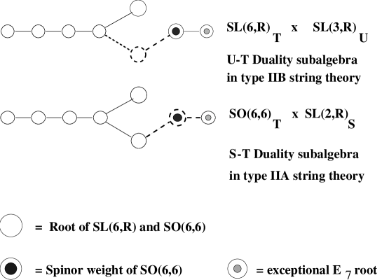
Figure 2:

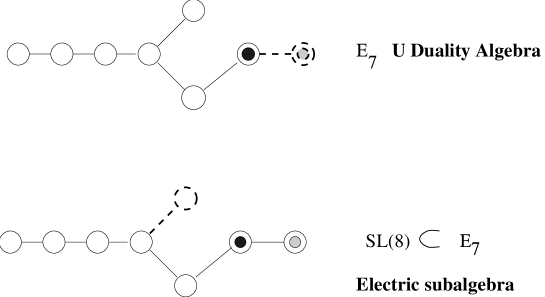
Figure 3:

From these embeddings occurring at the $E_{7}$ level, namely in $D=4$, one deduces the three embedding chains (19),(21),(22): it just suffices to peal off the last $\alpha_{r+1}$ roots one by one and also the $\beta$ root that occurs only in $D=4$. One observes that the appearance of the $\beta$ root is always responsible for an enhancement of the S–duality group. In the type IIA case this group is enhanced from $O(1,1)$ to $SL(2,{\rm I\kern-1.79993ptR})$ while in the type IIB case it is enhanced from the $SL(2,{\rm I\kern-1.79993ptR})_{U}$ already existing in $10$–dimensions to $SL(3,{\rm I\kern-1.79993ptR})$. Physically this occurs by combining the original dilaton field with the compactification radius of the latest compactified dimension.

3.3 String theory interpretation of the sequential embeddings: Type $IIA$, type $IIB$ and $M$ theory chains

We now turn to a closer analysis of the physical meaning of the embedding chains we have been illustrating.

Let us begin with the chain of eq.((21))that, as anticipated, is related with the type IIB interpretation of supergravity theory. The distinctive feature of this chain of embeddings is the presence of an addend $A_{1}$ that is already present in 10 dimensions. Indeed this $A_{1}$ is the Lie algebra of the $SL(2,R)_{\Sigma}$ symmetry of type $IIB$ D=10 superstring. We can name this group the U–duality symmetry $U_{10}$ in $D=10$. We can use the chain (21) to trace it in lower dimensions. Thus let us consider the decomposition

$$E_{r+1(r+1)} \rightarrow N_{r}\otimes SL(2,{\rm I\kern-1.79993ptR})$$

$$N_{r} = A_{r-1}\otimes O(1,1)$$ (35)

Obviously $N_{r}$ is not contained in the $T$-duality group $O(r,r)$ since the $NS$ tensor field $B_{\mu\nu}$ (which mixes with the metric under $T$-duality) and the $RR$–field $B^{c}_{\mu\nu}$ form a doublet with respect $SL(2,{\rm I\kern-1.79993ptR})_{U}$. In fact, $SL(2,{\rm I\kern-1.79993ptR})_{U}$ and $O(r,r)$ generate the whole U–duality group $E_{r+1(r+1)}$. The appropriate interpretation of the normaliser of $SL(2,R)_{\Sigma}$ in $E_{r+1(r+1)}$ is

$$N_{r}=O(1,1)\otimes SL(r,{\rm I\kern-1.79993ptR})\equiv GL(r,{\rm I\kern-1.79993ptR})$$ (36)

where $GL(r,{\rm I\kern-1.79993ptR})$ is the isometry group of the classical moduli space for the $T_{r}$ torus:

$$\frac{GL(r,{\rm I\kern-1.79993ptR})}{O(r)}.$$ (37)

The decomposition of the U–duality group appropriate for the type $IIB$ theory is

$$E_{r+1}\rightarrow U_{10}\otimes GL(r,{\rm I\kern-1.79993ptR})=SL(2,{\rm I\kern-1.79993ptR})_{U}\otimes O(1,1)\otimes SL(r,{\rm I\kern-1.79993ptR}).$$ (38)

Note that since $GL(r,{\rm I\kern-1.79993ptR})\supset O(1,1)^{r}$, this translates into $E_{r+1}\supset SL(2,{\rm I\kern-1.79993ptR})_{U}\otimes O(1,1)^{r}$. (In Type $IIA$, the corresponding chain would be $E_{r+1}\supset O(1,1)\otimes O(r,r)\supset O(1,1)^{r+1}$.) Note that while $SL(2,{\rm I\kern-1.79993ptR})$ mixes $RR$ and $NS$ states, $GL(r,{\rm I\kern-1.79993ptR})$ does not. Hence we can write the following decomposition for the solvable Lie algebra:

$$Solv\left(\frac{E_{r+1}}{H_{r+1}}\right) = Solv\left(\frac{GL(r,{\rm I\kern-1.79993ptR})}{O(r)}\otimes\frac{SL(2,{\rm I\kern-1.79993ptR})}{O(2)}\right)+\left(\frac{\bf r(r-1)}{\bf 2},{\bf 2}\right)\oplus{\bf X}\oplus{\bf Y}$$

$$\mbox{dim }Solv\left(\frac{E_{r+1}}{H_{r+1}}\right) = \frac{d(3d-1)}{2}+2+x+y.$$ (39)

where $x=\mbox{dim }{\bf X}$ counts the scalars coming from the internal part of the $4$–form $A^{+}_{{\mu}{\nu}{\rho}{\sigma}}$ of type IIB string theory. We have:

$$x=\left\{\matrix{0&r<4\cr\frac{r!}{4!(r-4)!}&r\geq 4\cr}\right.$$ (40)

and

$$y=\mbox{dim }{\bf Y}=\cases{\matrix{0&r<6\cr 2&r=6\cr}\cr}.$$ (41)

counts the scalars arising from dualising the two-index tensor fields in $r=6$.

For example, consider the $D=6$ case. Here the type $IIB$ decomposition is:

$$E_{5(5)}=\frac{O(5,5)}{O(5)\otimes O(5)}\rightarrow\frac{GL(4,{\rm I\kern-1.79993ptR})}{O(4)}\otimes\frac{SL(2,{\rm I\kern-1.79993ptR})}{O(2)}$$ (42)

whose compact counterpart is given by $O(10)\rightarrow SU(4)\otimes SU(2)\otimes U(1)$, corresponding to the decomposition: ${\bf 45}={\bf(15,1,1)}+{\bf(1,3,1)}+{\bf(1,1,1)}+{\bf(6,2,2)}+{\bf(1,1,2)}$. It follows:

$$Solv(\frac{E_{5(5)}}{O(5)\otimes O(5)})=Solv(\frac{GL(4,{\rm I\kern-1.79993ptR})}{O(4)}\otimes\frac{SL(2,{\rm I\kern-1.79993ptR})}{O(2)})+({\bf 6},{\bf 2})^{+}+({\bf 1},{\bf 1})^{+}.$$ (43)

where the factors on the right hand side parametrize the internal part of the metric $g_{ij}$, the dilaton and the $RR$ scalar ($\phi$, $\phi^{c}$), ($B_{ij}$, $B^{c}_{ij}$) and $A^{+}_{ijkl}$ respectively.

There is a connection between the decomposition ((35)) and the corresponding chains in M–theory. The type IIB chain is given by eq.((21)), namely by

$$E_{r+1(r+1)}\rightarrow SL(2,{\rm I\kern-1.79993ptR})\otimes GL(r,{\rm I\kern-1.79993ptR})$$ (44)

while the $M$ theory is given by eq.((22)), namely by

$$E_{r+1}\rightarrow O(1,1)\otimes SL(r+1,{\rm I\kern-1.79993ptR})$$ (45)

coming from the moduli space of $T^{11-D}=T^{r+1}$. We see that these decompositions involve the classical moduli spaces of $T^{r}$ and of $T^{r+1}$ respectively. Type $IIB$ and $M$ theory decompositions become identical if we decompose further $SL(r,{\rm I\kern-1.79993ptR})\rightarrow O(1,1)\times SL(r-1,{\rm I\kern-1.79993ptR})$ on the type $IIB$ side and $SL(r+1,{\rm I\kern-1.79993ptR})\rightarrow O(1,1)\otimes SL(2,{\rm I\kern-1.79993ptR})\otimes SL(r-1,{\rm I\kern-1.79993ptR})$ on the $M$-theory side. Then we obtain for both theories

$$E_{r+1}\rightarrow SL(2,{\rm I\kern-1.79993ptR})\times O(1,1)\otimes O(1,1)\otimes SL(r-1,{\rm I\kern-1.79993ptR}),$$ (46)

and we see that the group $SL(2,{\rm I\kern-1.79993ptR})_{U}$ of type $IIB$ is identified with the complex structure of the $2$-torus factor of the total compactification torus $T^{11-D}\rightarrow T^{2}\otimes T^{9-D}$.

Note that according to (34) in 8 and 4 dimensions, ($r=2$ and $6$) in the decomposition (46) there is the following enhancement:

$$SL(2,{\rm I\kern-1.79993ptR})\times O(1,1)\rightarrow SL(3,{\rm I\kern-1.79993ptR})\quad(\mbox{for}\,r=2,6)$$ (47)

$$\left\{\matrix{O(1,1)&\rightarrow&SL(2,{\rm I\kern-1.79993ptR})\quad(\mbox{for}\,r=2)\cr SL(5,{\rm I\kern-1.79993ptR})\times O(1,1)&\rightarrow&SL(6,{\rm I\kern-1.79993ptR})\quad(\mbox{for}\,r=6)\cr}\right.$$ (48)

Finally, by looking at fig.(4) let us observe that $E_{7(7)}$ admits also a subgroup $SL(2,{\rm I\kern-1.79993ptR})_{T}$ $\otimes(SO(5,5)_{S}$ $\equiv E_{5(5)})$ where the $SL(2,{\rm I\kern-1.79993ptR})$ factor is a T–duality group, while the factor $(SO(5,5)_{S}$ $\equiv E_{5(5)})$ is an S–duality group which mixes RR and NS states.

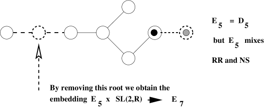
Figure 4:

4 The maximal abelian ideals ${\cal A}_{r+1}\subset Solv_{r+1}$ of the solvable Lie algebra

It is interesting to work out the maximal abelian ideals ${\cal A}_{r+1}\subset Solv_{r+1}$ of the solvable Lie algebras generating the scalar manifolds of maximal supergravity in dimension $D=10-r$. The maximal abelian ideal of a solvable Lie algebra is defined as the maximal subset of nilpotent generators commuting among themselves. From a physical point of view this is the largest abelian Lie algebra that one might expect to be able to gauge in the supergravity theory. Indeed, as it turns out, the number of vector fields in the theory is always larger or equal than $\mbox{dim}{\cal A}_{r+1}$. Actually, as we are going to see, the gaugeable maximal abelian algebra is always a proper subalgebra ${\cal A}^{gauge}_{r+1}\subset{\cal A}_{r+1}$ of this ideal.

The criteria to determine ${\cal A}^{gauge}_{r+1}$ will be discussed in the next section. In the present section we derive ${\cal A}_{r+1}$ and we explore its relation with the space of vector fields in one dimension above the dimension we each time consider. From such analysis we obtain a filtration of the solvable Lie algebra which provides us with a canonical polynomial parametrization of the supergravity scalar coset manifold $U_{r+1}/H_{r+1}$

4.1 The maximal abelian ideal from an algebraic viewpoint

Algebraically the maximal abelian ideal can be characterized by looking at the decomposition of the U–duality algebra $E_{r+1(r+1)}$ with respect to the U–duality algebra in one dimension above. In other words we have to consider the decomposition of $E_{r+1(r+1)}$ with respect to the subalgebra $E_{r(r)}\,\otimes\,O(1,1)$. This decomposition follows a general pattern which is given by the next formula:

$$\mbox{adj }E_{r+1(r+1)}\,=\,\mbox{adj }E_{r(r)}\,\oplus\,\mbox{adj }O(1,1)\,\oplus({\rm I\kern-1.79993ptD}^{+}_{r}\oplus{\rm I\kern-1.79993ptD}^{-}_{r})$$ (49)

where ${\rm I\kern-1.79993ptD}^{+}_{r}$ is at the same time an irreducible representation of the U–duality algebra $E_{r(r)}$ in $D+1$ dimensions and coincides with the maximal abelian ideal

$${\rm I\kern-1.79993ptD}^{+}_{r}\,\equiv\,{\cal A}_{r+1}\,\subset\,Solv_{(r+1)}$$ (50)

of the solvable Lie algebra we are looking for. In eq. (49) the subspace ${\rm I\kern-1.79993ptD}^{-}_{r}$ is just a second identical copy of the representation ${\rm I\kern-1.79993ptD}^{+}_{r}$ and it is made of negative rather than of positive weights of $E_{r(r)}$. Furthermore ${\rm I\kern-1.79993ptD}^{+}_{r}$ and ${\rm I\kern-1.79993ptD}^{-}_{r}$ correspond to the eigenspaces belonging respectively to the eigenvalues $\pm 1$ with respect to the adjoint action of the S–duality group $O(1,1)$.

4.2 The maximal abelian ideal from a physical perspective: the vector fields in one dimension above and translational symmetries

Here, we would like to show that the dimension of the abelian ideal in $D$ dimensions is equal to the number of vectors in dimensions $D+1$. Denoting the number of compactified dimensions by $r$ (in string theory, $r=10-D$), we will label the $U$-duality group in $D$ dimensions by $U_{D}=E_{11-D}=E_{r+1}$. The $T$-duality group is $O(r,r)$, while the $S$-duality group is $O(1,1)$ in dimensions higher than four, $SL(2,R)$ in $D=4$ (and it is inside $O(8,8)$ in $D=3$).

It follows from (49) that the total dimension of the abelian ideal is given by

$${\rm dim}\,{\cal A}_{D}\,\equiv\,{\rm dim}\,{\cal A}_{r+1}\,\equiv\,{\rm dim}\,{\rm I\kern-1.79993ptD}_{r}$$ (51)

where ${\rm I\kern-1.79993ptD}_{r}$ is a representation of $U_{D+1}$ pertaining to the vector fields. According to (49) we have (for $D\geq 4$):

$$\mbox{adj }U_{D}=\mbox{adj }U_{D+1}\oplus{\bf 1}\oplus({\bf 2},{\rm I\kern-1.79993ptD}_{r}).$$ (52)

This is just an immediate consequence of the embedding chain (18) which at the first level of iteration yields $E_{r+1}\rightarrow E_{r}\times O(1,1)$. For example, under $E_{7}\rightarrow E_{6}\times O(1,1)$ we have the branching rule: ${\rm adj}\,E_{7}={\rm adj}\,E_{6}+{\bf 1}+({\bf 2},{\bf 27})$ and the abelian ideal is given by the ${\bf 27^{+}}$ representation of the $E_{6(6)}$ group. The $70$ scalars of the $D=4,N=8$ theory are naturally decomposed as ${\bf 70}={\bf 42}+{\bf 1}+{\bf 27^{+}}$. To see the splitting of the abelian ideal scalars into $NS$ and $RR$ sectors, one has to consider the decomposition of $U_{D+1}$ under the T–duality group $T_{D+1}=O(r-1,r-1)$, namely the second iteration of the embedding chain (18): $E_{r+1}\rightarrow O(1,1)\times O(r-1,r-1)$. Then the vector representation of $O(r-1,r-1)$ gives the $NS$ sector, while the spinor representation yields the $RR$ sector. The example of $E_{7}$ considered above is somewhat exceptional, since we have ${\bf 27}\rightarrow({\bf 10}+{\bf 1}+{\bf 16})$. Here in addition to the expected ${\bf 10}$ and ${\bf 16}$ of $O(5,5)$ we find an extra $NS$ scalar: physically this is due to the fact that in four dimensions the two-index antisymmetric tensor field $B_{\mu\nu}$ is dual to a scalar, algebraically this generator is associated with the exceptional root $\sqrt{2}\epsilon_{7}$. To summarize, the $NS$ and $RR$ sectors are separately invariant under $O(r,r)$ in $D=10-r$ dimensions, while the abelian $NS$ and $RR$ sectors are invariant under $O(r-1,r-1)$. The standard parametrization of the $U_{D}/H_{D}$ and $U_{D+1}/H_{D+1}$ cosets gives a clear illustration of this fact:

$$\frac{U_{D}}{H_{D}}\sim(\frac{U_{D+1}}{H_{D+1}},r_{D+1},{\bf V}_{r}^{D+1}).$$ (53)

Here $r_{D+1}$ stands for the compactification radius, and ${\bf V}_{r}^{D+1}$ are the compactified vectors yielding the abelian ideal in $D$ dimensions.

Note that:

$$\mbox{adj}\,H_{D}=\mbox{adj}\,H_{D+1}\,+\,\mbox{adj}\,\mbox{Irrep}\,U_{D+1}$$ (54)

so it appears that the abelian ideal forms a representation not only of $U_{D+1}$ but also of the compact isotropy subgroup $H_{D+1}$ of the scalar coset manifold.

In the above $r=6$ example we find ${\rm adj}\,SU(8)={\rm adj}\,USp(8)\oplus{\bf 27^{-}}$, $\Longrightarrow$ ${\bf 63}={\bf 36}+{\bf 27^{-}}$.

4.3 Maximal abelian ideal and brane wrapping

Now we would like to turn to a uniform counting of the ideal dimension in diverse space–time dimensions. The fact that the ($D+1$)-dimensional vectors have $0$-branes as electric sources (or equivalently, ($D-3$)-branes as magnetic ones) reduces the analysis of the $RR$ sector to a simple exercise in counting the ways of wrapping higher dimensional $d$-branes around the cycles of the compact manifold. This procedure spares one from doing a case-by-case counting and worrying about the scalars arising from the dualization of the tensor fields. It also easily generalizes for manifolds other then $T^{r}$. The latter choice corresponds to the case of maximal preserved supersymmetry, for which the counting is presented here.

Starting from Type $IIA$ theory with 0, 2, 4, 6 -Dbranes [23], the total number of ($D+1$)-dimensional 0-Dbranes (i.e. the maximal abelian ideal in $D$–dimensions) is obtained by wrapping the Dbranes around the even cycles of the ($9-D$)-dimensional torus. One gets:

$$n_{{\cal A}}^{RR}=\sum_{k}b_{2k}(T^{9-D})=2^{8-D}$$ (55)

where $b_{2k}$ are the Betti numbers. The same result is obtained by counting the magnetic sources: in this case the sum is taken over alternating series of even (odd) cohomology for $9-D$ even (odd), since the $6$-Dbrane is wrapped on the $(9-D)$-dimensional cycle of $T^{9-D}$, the $4$-Dbrane on $(7-D)$-dimensional cycles and so on. Note that wrapping Dbranes around the cycles of the same dimensions as above but on a $T^{10-D}$ yields the total number of the $RR$ scalars in $D$ dimensions.

The type $IIB$ story is exactly the same with the even cycles replaced by the odd ones. The only little subtlety is in going from ten dimensions to nine - there is no $0$-Dbrane in type $IIB$, but instead there is a $RR$ scalar in the ideal already in ten dimensions, since the $U$-duality group is non-trivial. Of course the results agree on $T^{r}$ as they should on any manifold with a vanishing Euler number.

The $NS$ parts of the ideal ($(D-3)$-branes in ($D+1$)-dimensions) are obtained either by wrapping the ten-dimensional fivebrane or as magnetic sources for Kaluza-Klein vectors (note that for the $NS$ part, the reasonings for Type $IIA$ and $IIB$ are identical). The former are the fivebrane wrapped on $(8-D)$ cycles of $T^{9-D}$ (there are $(9-D)$ of them), while the latter are given by the same number since it is the number of the Kaluza–Klein vectors (number of $1$-cycles). Thus

$$n_{{\cal A}}^{NS}=2b_{1}(T^{9-D})=2(9-D).$$ (56)

The only exception to this formula is the $D=4$ case where, as discussed above, we have to add an extra scalar due to the $B_{\mu\nu}$ field.

5 Gauging

In this last section we will consider the problem of gauging some isometries of the coset $G/H$ in the framework of solvable Lie algebras.

In particular we will consider in more detail the gauging of maximal compact groups and the gauging of nilpotent abelian (translational) isometries.

This procedure is a way of obtaining partial supersymmetry breaking in extended supergravities [21],[24],[25] and it may find applications in the context of non perturbative phenomena in string and M-theories.

Let us consider the left–invariant 1–form $\Omega=L^{-1}dL$ of the coset manifold $U_{D}/H_{D}$, where $L$ is the coset representative.

The gauging procedure [26] amounts to the replacement of $dL$ with the gauge covariant differential $\nabla L$ in the definition of the left–invariant 1–form $\Omega=L^{-1}dL$:

$$\Omega\rightarrow\widehat{\Omega}=L^{-1}\nabla L=L^{-1}(d+A)L=\Omega+L^{-1}AL$$ (57)

As a consequence $\widehat{\Omega}$ is no more a flat connection, but its curvature is given by:

$$R(\widehat{\Omega})=d\widehat{\Omega}+\widehat{\Omega}\wedge\widehat{\Omega}=L^{-1}{\cal F}L\equiv L^{-1}(dA+A\wedge A)L=L^{-1}(F^{I}T_{I}+L^{I}_{AB}T_{I}\overline{\psi}^{A}\psi^{B})L$$ (58)

where $F^{I}$ is the gauged supercovariant 2–form and $T_{I}$ are the generators of the gauge group embedded in the U–duality representation of the vector fields.

Indeed, by very definition, under the full group $E_{r+1(r+1)}$ the gauge vectors are contained in the representation ${\rm I\kern-1.79993ptD}_{r+1}$. Yet, with respect to the gauge subgroup they must transform in the adjoint representation, so that ${\cal G}_{D}$ has to be chosen in such a way that:

$${\rm I\kern-1.79993ptD}_{r+1}\,\stackrel{{\scriptstyle{\cal G}_{D}}}{{\longrightarrow}}\,\mbox{adj}\,{\cal G}_{D}\,\oplus\,\mbox{rep}\,{\cal G}_{D}$$ (59)

where $\mbox{rep}\,{\cal G}_{D}$ is some other representation of ${\cal G}_{D}$ contained in the above decomposition.

It is important to remark that vectors which are in $\mbox{rep}{\cal G}_{D}$ (i.e. vectors which do not gauge ${\cal G}_{D}$) may be required, by consistence of the theory [27], to appear through their duals $(D-3)$–forms, as for instance happens for $D=5$ [28]. In an analogous way $p$–form potentials ($p\neq 1$) which are in non trivial representations of ${\cal G}_{D}$ may also be required to appear through their duals $(D-p-2)$–potentials, as is the case in $D=7$ for $p=2$ [29].

The charges and the boosted structure constants discussed in the next subsection can be retrieved from the two terms appearing in the last expression of eq. (58)

5.1 Filtration of the $E_{r+1}$ root space, canonical parametrization of the coset representatives and boosted structure constants

As it has already been emphasized in the introduction, the complete structure of $N>2$ supergravity in diverse dimensions is fully encoded in the local differential geometry of the scalar coset manifold $U_{D}/H_{D}$. All the couplings in the Lagrangian are described in terms of the metric, the connection and the coset representative (2) of $U_{D}/H_{D}$. A particularly significant consequence of extended supersymmetry is that the fermion masses and the scalar potential the theory can develop occur only as a consequence of the gauging and can be extracted from a decomposition in terms of irreducible $H_{D}$ representations of the boosted structure constants[30] [26]. Let us define these latter. Let ${\rm I\kern-1.79993ptD}_{r+1}$ be the irreducible representation of the $U_{D}$ U–duality group pertaining to the vector fields and denote by ${\vec{\bf w}}_{\Lambda}$ a basis for ${\rm I\kern-1.79993ptD}_{r+1}$:

$$\forall{\vec{\bf v}}\,\in\,{\rm I\kern-1.79993ptD}_{r+1}\qquad:\qquad{\vec{v}}\,=\,v^{\Lambda}\,{\vec{\bf w}}_{\Lambda}$$ (60)

In the case we consider of maximal supergravity theories, where the U–duality groups are given by $E_{r+1(r+1)}$ the basis vectors ${\vec{bfw}}_{\Lambda}$ can be identified with the $56$ weights of the fundamental $E_{7(7)}$ representation or with the subsets of this latter corresponding to the irreducible representations of its $E_{r+1(r+1)}$ subgroups, according to the branching rules:

$${\bf 56}{\stackrel{{\scriptstyle E_{6}}}{{\longrightarrow}}}\cases{{\bf 27+1}{\stackrel{{\scriptstyle E_{5}}}{{\longrightarrow}}}\cases{{\bf 16}{\stackrel{{\scriptstyle E_{4}}}{{\longrightarrow}}}{\bf\dots}\cr{\bf 10}{\stackrel{{\scriptstyle E_{4}}}{{\longrightarrow}}}{\bf\dots}\cr{\bf 1+1}{\stackrel{{\scriptstyle E_{4}}}{{\longrightarrow}}}{\bf\dots}\cr}\cr{\bf 27+1}{\stackrel{{\scriptstyle E_{5}}}{{\longrightarrow}}}\cases{{\bf 16}{\stackrel{{\scriptstyle E_{4}}}{{\longrightarrow}}}{\bf\dots}\cr{\bf 10}{\stackrel{{\scriptstyle E_{4}}}{{\longrightarrow}}}{\bf\dots}\cr{\bf 1+1}{\stackrel{{\scriptstyle E_{4}}}{{\longrightarrow}}}{\bf\dots}\cr}\cr}$$ (61)

Let:

$$<~{},~{}>\quad:\quad{\rm I\kern-1.79993ptD}_{r+1}\,\times{\rm I\kern-1.79993ptD}_{r+1}\,\longrightarrow\,{\rm I\kern-1.79993ptR}$$ (62)

denote the invariant scalar product in ${\rm I\kern-1.79993ptD}_{r+1}$ and let ${\vec{\bf w}}^{\Sigma}$ be a dual basis such that

$$<{\vec{\bf w}}^{\Sigma},{\vec{\bf w}}_{\Lambda}>\,=\,\delta^{\Sigma}_{\Lambda}$$ (63)

Consider then the ${\rm I\kern-1.79993ptD}_{r+1}$ representation of the coset representative (2):

$$L(\phi)\quad:\quad|{\vec{\bf w}}_{\Lambda}>\,\longrightarrow L(\phi)_{\Lambda}^{\Sigma}\,|{\vec{\bf w}}_{\Sigma}>,$$ (64)

and let $T^{I}$ be the generators of the gauge algebra ${\cal G}_{D}\,\subset E_{r+1(r+1)}$.

The only admitted generators are those with index $\Lambda=I\,\in\,{adj}\,{\cal G}_{D}$, and there are no gauge group generators with index $\Lambda\,\in\,\mbox{rep}\,{\cal G}_{D}$. Given these definitions the boosted structure constants are the following three–linear $3$–tensors in the coset representatives:

$$\,\hbox{$\vrule height=6.45831pt,width=0.4pt,depth=0.0pt\kern-3.00003pt{\rm C}$}_{\Sigma\Gamma}^{\Lambda}\left(\phi\right)\,\equiv\,\sum_{I=1}^{{\rm dim}{\cal G}_{D}}\,<{\vec{\bf w}}^{\Lambda}\,,\,L^{-1}\left(\phi\right)\,T_{I}\,L\left(\phi\right)\,{\vec{\bf w}}_{\Sigma}>\,<{\vec{\bf w}}^{I}\,,\,L\left(\phi\right){\vec{\bf w}}_{\Gamma}>$$ (65)

and by decomposing them into irreducible $H_{r+1}$ representations we obtain the building blocks utilized by supergravity in the fermion shifts, in the fermion mass–matrices and in the scalar potential.

In an analogous way, the charges appearing in the gauged covariant derivatives are given by the following general form:

$$Q_{I\Sigma}^{\Lambda}\,\equiv\,<{\vec{\bf w}}^{\Lambda}\,,\,L^{-1}\left(\phi\right)\,T_{I}\,L\left(\phi\right)\,{\vec{\bf w}}_{\Sigma}>$$ (66)

The coset representative $L\left(\phi\right)$ can be written in a canonical polynomial parametrization which should give a simplifying tool in mastering the scalar field dependence of all physical relevant quantities. This includes, besides mass matrices, fermion shifts and scalar potential, also the central charges [31].

The alluded parametrization is precisely what the solvable Lie algebra analysis produces.

To this effect let us decompose the solvable Lie algebra of $E_{7(7)}/SU(8)$ in a sequential way utilizing eq. (49). Indeed we can write the equation:

$$Solv(E_{7(7)})={\cal H}_{7}\oplus\Phi^{+}(E_{7})$$ (67)

where $\Phi^{+}(E_{7})$ is the $63$ dimensional positive part of the $E_{7}$ root space. By repeatedly using eq. (49) we obtain:

$$\Phi^{+}(E_{7})=\Phi^{+}(E_{2})\oplus{\rm I\kern-1.79993ptD}^{+}_{2}\oplus{\rm I\kern-1.79993ptD}^{+}_{3}\oplus{\rm I\kern-1.79993ptD}^{+}_{4}\oplus{\rm I\kern-1.79993ptD}^{+}_{5}\oplus{\rm I\kern-1.79993ptD}^{+}_{6}$$ (68)

where $\Phi^{+}(E_{2})$ is the one–dimensional root space of the U–duality group in $D=9$ and ${\rm I\kern-1.79993ptD}^{+}_{r+1}$ are the weight-spaces of the $E_{r+1}$ irreducible representations to which the vector field in $D=10-r$ are assigned. Alternatively, as we have already explained, ${\cal A}_{r+2}\equiv{\rm I\kern-1.79993ptD}^{+}_{r+1}$ are the maximal abelian ideals of the U–duality group in $E_{r+2}$ in $D=10-r-1$ dimensions.

We can easily check that the dimensions sum appropriately as follows from:

$$\mbox{dim}\,\Phi^{+}(E_{7})\, = {63}$$

$$\mbox{dim}\,\Phi^{+}(E_{2})\, = {1}\quad\quad~{}\mbox{dim}\,{\rm I\kern-1.79993ptD}^{+}_{2}\,={3}$$

$$\mbox{dim}\,{\rm I\kern-1.79993ptD}^{+}_{3}\, = {6}\quad\quad~{}\mbox{dim}\,{\rm I\kern-1.79993ptD}^{+}_{4}\,={10}$$

$$\mbox{dim}\,{\rm I\kern-1.79993ptD}^{+}_{5}\, = {16}\quad\quad\mbox{dim}\,{\rm I\kern-1.79993ptD}^{+}_{4}\,={27}$$

Relying on eq. (67), (68) we can introduce a canonical set of scalar field variables:

$$\phi^{i} \longrightarrow Y_{i}\,\in{\cal H}\quad\quad i=1,\dots\,r$$

$$\tau^{i}_{k} \longrightarrow \,D^{(k)}_{i}\,\in{\rm I\kern-1.79993ptD}_{k}\quad i=1,\dots\,\mbox{dim }\,{\rm I\kern-1.79993ptD}_{k}\quad(k=2,\dots,6)$$

$$\tau_{1} \longrightarrow {\rm I\kern-1.79993ptD}_{1}\,\equiv\,E_{2}$$ (70)

and adopting the short hand notation:

$$\phi\cdot{\cal H} \equiv \phi^{i}\,Y_{i}$$

$$\tau_{k}\cdot{\rm I\kern-1.79993ptD}_{k} \equiv \tau^{i}_{k}\,D^{(k)}_{i}$$

we can write the coset representative for maximal supergravity in dimension $D=10-r$ as:

$$L = \exp\left[\phi\cdot{\cal H}\right]\,\prod_{k=1}^{r}\,\exp\left[\tau_{k}\cdot{\rm I\kern-1.79993ptD}_{k}\right]$$ (72)

$$= \prod_{j=1}^{r+1}S^{i}\,\prod_{k=1}^{r}\,\left({1}+\tau_{r}\cdot{\rm I\kern-1.79993ptD}_{r}\right)$$

The last line follows from the abelian nature of the ideals ${\rm I\kern-1.79993ptD}_{k}$ and from the position:

$$S^{i}\,\equiv\,\exp[\phi^{i}Y_{i}]$$ (73)

All entries of the matrix $L$ are therefore polynomials of order at most $2\,r\,+\,1$ in the $S^{i},\tau^{i}_{k},\tau_{1}$ “canonical” variables. Furthermore when the gauge group is chosen within the maximal abelian ideal it is evident from the definition of the boosted structure constants (65) that they do not depend on the scalar fields associated with the generators of the same ideal. In such gauging one has therefore a flat direction of the scalar potential for each generator of the maximal abelian ideal.

In the next section we turn to considering the possible gaugings more closely.

5.2 Gauging of compact and translational isometries

A necessary condition for the gauging of a subgroup ${\cal G}_{D}\subset U_{D}$ is that the representation of the vectors ${\rm I\kern-1.79993ptD}_{r+1}$ must contain $\mbox{adj}{\cal G}_{D}$. Following this prescription, the list of maximal compact gaugings ${\cal G}_{D}$ in any dimensions is obtained in the third column of Table 3. In the other columns we list the $U_{D}$-duality groups, their maximal compact subgroups and the left-over representations for vector fields.

Table 3: Maximal gauged compact groups

$D$	$U_{D}$	$H_{D}$	${\cal G}_{D}$	$\mbox{rep}{\cal G}_{D}$
9	$SL(2,{\rm I\kern-1.79993ptR})\times O(1,1)$	$O(2)$	$O(2)$	2
8	$SL(3,{\rm I\kern-1.79993ptR})\times SL(2,{\rm I\kern-1.79993ptR})$	$O(3)\times O(2)$	$O(3)$	$3$
7	$SL(5,{\rm I\kern-1.79993ptR})$	$USp(4)$	$O(5)\sim USp(4)$	0
6	$O(5,5)$	$USp(4)\times USp(4)$	$O(5)$	$5+1$
5	$E_{6,(6)}$	$USp(8)$	$O(6)\sim SU(4)$	$2\times 6$
4	$E_{7(7)}$	$SU(8)$	$O(8)$	0

Table 4: Transformation properties under ${\cal G}_{D}$ of 2- and 3-forms

$D$	$\mbox{rep}\,B_{\mu\nu}$	$\mbox{rep}\,A_{\mu\nu\rho}$
9	2	0
8	3	0
7	0	5
6	5	0
5	$2\times 6$	0

We notice that, for any $D$, there are $p$–forms ($p$ =1,2,3) which are charged under the gauge group ${\cal G}_{D}$. Consistency of these theories requires that such forms become massive. It is worthwhile to mention how this can occur in two variants of the Higgs mechanism. Let us define the (generalized) Higgs mechanism for a $p$–form mass generation through the absorption of a massless ($p-1$)–form (for $p=1$ this is the usual Higgs mechanism). The first variant is the anti-Higgs mechanism for a $p$–form [32], which is its absorption by a massless ($p+1$)–form. It is operating, for $p=1$, in $D=5,6,8,9$ for a sextet of $SU(4)$, a quintet of $SO(5)$, a triplet of $SO(3)$ and a doublet of $SO(2)$, respectively. The second variant is the self–Higgs mechanism [27], which only exists for $p=(D-1)/2$, $D=4k-1$. This is a massless $p$–form which acquires a mass through a topological mass term and therefore it becomes a massive “chiral” $p$–form. The latter phenomena was shown to occur in $D=3$ and $7$. It is amazing to notice that the representation assignments dictated by $U$–duality for the various $p$–forms is precisely that needed for consistency of the gauging procedure (see Table 4).

The other compact gaugings listed in Table 3 are the $D=4$ [33] and $D=8$ cases [34].

It is possible to extend the analysis of gauging semisimple groups also to the case of solvable Lie groups [15]. For the maximal abelian ideals of $Solv(U_{D}/H_{D})$ this amounts to gauge an $n$–dimensional subgroup of the translational symmetries under which at least $n$ vectors are inert. Indeed the vectors the set of vectors that can gauge an abelian algebra (being in its adjoint representation) must be neutral under the action of such an algebra. We find that in any dimension $D$ the dimension of this abelian group $\mbox{dim}{\cal G}_{abel}$ is given precisely by ${\rm dim}(\mbox{rep}{\cal G}_{D})$ which appear in the decomposition of ${\rm I\kern-1.79993ptD}_{r+1}$ under $O(r+1)$. We must stress that this criterium gives a necessary but not sufficient condition for the existence of the gauging of an abelian isometry group, consistent with supersymmetry.

Table 5: Decomposition of fields in representations of the compact group ${\cal G}_{D}=O(11-D)$

	vect. irrep	adj($O(11-D)$)	${\cal A}$	$\mbox{dim}{\cal G}_{abel}$
$D=9$	$1+2$	1	1	1
$D=8$	$3+3$	3	3	3
$D=7$	$6+4$	6	6	4
$D=6$	$10+5+1$	10	10	$5+1$
$D=5$	$15+6+6$	15	$15+1$	$6+6$
$D=4$	$(21+7)\times 2$	21	$21+1\times 6$	7

Conclusions

In this paper we have analyzed some properties of the effective theories of type II strings and M–theory in the framework of solvable Lie algebras.

Particular attention has been given to the classification of R–R and N–S sectors as well as to the translational symmetries of the classical moduli space.

The problem of gauging isometries in this framework has been reconsidered with emphasis to its interplay with U–duality.

It is hoped that further developments of these results may find applications in the study of non perturbative dynamics of string theories, such as the finding of new vacua and the study of supersymmetry breaking.

Appendix A: Explicit pairing between Lie algebra roots and fields

By referring to the toroidal dimensional reduction of type IIA superstring and Tables 1, 2, it is straightforward to establish a correspondence between the scalar fields of either Neveu–Schwarz or Ramond–Ramond type emerging at each step of the sequential compactification and the positive roots of $\Phi^{+}(E_{7})$, distributed into the ${\rm I\kern-1.79993ptD}^{+}_{r+1}$ subspaces. This gives rise to the following list of solvable algebra generators. The roots of $SO(6,6)$ are associated with N–S fields, the spinor weights of $SO(6,6)$ are associated with R–R fields.

The abelian ideal in $D=8$ $E_{3}\supset{\cal A}_{3}\equiv{\rm I\kern-1.79993ptD}^{+}_{2}$ is given by the roots:

${\rm I\kern-1.79993ptD}^{+}_{2}=$

$$B_{9,10}~{}\rightarrow~{}D_{2}(1) = \{0,0,0,0,1,1,0\}$$

$$g_{9,10}~{}\rightarrow~{}D_{2}(2) = \{0,0,0,0,1,-1,0\}$$

$$A_{9}~{}\rightarrow~{}D_{2}(3) = \{-{1\over 2},-{1\over 2},-{1\over 2},-{1\over 2},{1\over 2},{1\over 2},{1\over{{\sqrt{2}}}}\}$$ (74)

The abelian ideal in $D=7$ $E_{4}\supset{\cal A}_{4}\equiv{\rm I\kern-1.79993ptD}^{+}_{3}$ is given by the roots:

${\rm I\kern-1.79993ptD}^{+}_{3}=$

$$B_{8,9}~{}\rightarrow~{}D_{3}(1) = \{0,0,0,1,1,0,0\}$$

$$g_{8,9}~{}\rightarrow~{}D_{3}(2) = \{0,0,0,1,-1,0,0\}$$

$$B_{8,10}~{}\rightarrow~{}D_{3}(3) = \{0,0,0,1,0,1,0\}$$

$$g_{8,10}~{}\rightarrow~{}D_{3}(4) = \{0,0,0,1,0,-1,0\}$$

$$A_{8}~{}\rightarrow~{}D_{3}(5) = \{-{1\over 2},-{1\over 2},-{1\over 2},{1\over 2},{1\over 2},-{1\over 2},{1\over{{\sqrt{2}}}}\}$$

$$A_{8,9,10}~{}\rightarrow~{}D_{3}(6) = \{-{1\over 2},-{1\over 2},-{1\over 2},{1\over 2},-{1\over 2},{1\over 2},{1\over{{\sqrt{2}}}}\}$$ (75)

The abelian ideal in $D=6$ $E_{5}\supset{\cal A}_{5}\equiv{\rm I\kern-1.79993ptD}^{+}_{4}$ is given by the roots:

${\rm I\kern-1.79993ptD}^{+}_{4}=$

$$B_{7,8}~{}\rightarrow~{}D_{4}(1) = \{0,0,1,1,0,0,0\}$$

$$g_{7,8}~{}\rightarrow~{}D_{4}(2) = \{0,0,1,-1,0,0,0\}$$

$$B_{7,9}~{}\rightarrow~{}D_{4}(3) = \{0,0,1,0,1,0,0\}$$

$$g_{7,9}~{}\rightarrow~{}D_{4}(4) = \{0,0,1,0,-1,0,0\}$$

$$B_{7,10}~{}\rightarrow~{}D_{4}(5) = \{0,0,1,0,0,1,0\}$$

$$g_{7,10}~{}\rightarrow~{}D_{4}(6) = \{0,0,1,0,0,-1,0\}$$

$$A_{7,9,10}~{}\rightarrow~{}D_{4}(7) = \{-{1\over 2},-{1\over 2},{1\over 2},{1\over 2},-{1\over 2},-{1\over 2},{1\over{{\sqrt{2}}}}\}$$

$$A_{7,8,10}~{}\rightarrow~{}D_{4}(8) = \{-{1\over 2},-{1\over 2},{1\over 2},-{1\over 2},{1\over 2},-{1\over 2},{1\over{{\sqrt{2}}}}\}$$

$$A_{7,8,9}~{}\rightarrow~{}D_{4}(9) = \{-{1\over 2},-{1\over 2},{1\over 2},-{1\over 2},-{1\over 2},{1\over 2},{1\over{{\sqrt{2}}}}\}$$

$$A_{7}~{}\rightarrow~{}D_{4}(10) = \{-{1\over 2},-{1\over 2},{1\over 2},{1\over 2},{1\over 2},{1\over 2},{1\over{{\sqrt{2}}}}\}$$ (76)

The abelian ideal in $D=5$ $E_{6}\supset{\cal A}_{6}\equiv{\rm I\kern-1.79993ptD}^{+}_{5}$ is given by the roots:

${\rm I\kern-1.79993ptD}^{+}_{5}=$

$$B_{6,7}~{}\rightarrow~{}D_{5}(1) = \{0,1,1,0,0,0,0\}$$

$$g_{6,7}~{}\rightarrow~{}D_{5}(2) = \{0,1,-1,0,0,0,0\}$$

$$B_{6,8}~{}\rightarrow~{}D_{5}(3) = \{0,1,0,1,0,0,0\}$$

$$g_{6,8}~{}\rightarrow~{}D_{5}(4) = \{0,1,0,-1,0,0,0\}$$

$$B_{6,9}~{}\rightarrow~{}D_{5}(5) = \{0,1,0,0,1,0,0\}$$

$$g_{6,9}~{}\rightarrow~{}D_{5}(6) = \{0,1,0,0,-1,0,0\}$$

$$B_{6,10}~{}\rightarrow~{}D_{5}(7) = \{0,1,0,0,0,1,0\}$$

$$g_{6,10}~{}\rightarrow~{}D_{5}(8) = \{0,1,0,0,0,-1,0\}$$

$$A_{6,8,9}~{}\rightarrow~{}D_{5}(9) = \{-{1\over 2},{1\over 2},{1\over 2},-{1\over 2},-{1\over 2},-{1\over 2},{1\over{{\sqrt{2}}}}\}$$

$$A_{6,7,9}~{}\rightarrow~{}D_{5}(10) = \{-{1\over 2},{1\over 2},-{1\over 2},{1\over 2},-{1\over 2},-{1\over 2},{1\over{{\sqrt{2}}}}\}$$

$$A_{6,7,8}~{}\rightarrow~{}D_{5}(11) = \{-{1\over 2},{1\over 2},-{1\over 2},-{1\over 2},{1\over 2},-{1\over 2},{1\over{{\sqrt{2}}}}\}$$

$$A_{\mu\nu\rho}~{}\rightarrow~{}D_{5}(12) = \{-{1\over 2},{1\over 2},-{1\over 2},-{1\over 2},-{1\over 2},{1\over 2},{1\over{{\sqrt{2}}}}\}$$

$$A_{6,7,10}~{}\rightarrow~{}D_{5}(13) = \{-{1\over 2},{1\over 2},-{1\over 2},{1\over 2},{1\over 2},{1\over 2},{1\over{{\sqrt{2}}}}\}$$

$$A_{6,8,10}~{}\rightarrow~{}D_{5}(14) = \{-{1\over 2},{1\over 2},{1\over 2},-{1\over 2},{1\over 2},{1\over 2},{1\over{{\sqrt{2}}}}\}$$

$$A_{6,9,10}~{}\rightarrow~{}D_{5}(15) = \{-{1\over 2},{1\over 2},{1\over 2},{1\over 2},-{1\over 2},{1\over 2},{1\over{{\sqrt{2}}}}\}$$

$$A_{6}~{}\rightarrow~{}D_{5}(16) = \{-{1\over 2},{1\over 2},{1\over 2},{1\over 2},{1\over 2},-{1\over 2},{1\over{{\sqrt{2}}}}\}$$ (77)

The abelian ideal in $D=4$ $E_{7}\supset{\cal A}_{7}\equiv{\rm I\kern-1.79993ptD}^{+}_{6}$ is given by the roots:

${\rm I\kern-1.79993ptD}^{+}_{6}=$

$$B_{5,6}~{}\rightarrow~{}D_{6}(1) = \{1,1,0,0,0,0,0\}$$

$$g_{5,6}~{}\rightarrow~{}D_{6}(2) = \{1,-1,0,0,0,0,0\}$$

$$B_{5,7}~{}\rightarrow~{}D_{6}(3) = \{1,0,1,0,0,0,0\}$$

$$g_{5,7}~{}\rightarrow~{}D_{6}(4) = \{1,0,-1,0,0,0,0\}$$

$$B_{5,8}~{}\rightarrow~{}D_{6}(5) = \{1,0,0,1,0,0,0\}$$

$$g_{5,8}~{}\rightarrow~{}D_{6}(6) = \{1,0,0,-1,0,0,0\}$$

$$B_{5,9}~{}\rightarrow~{}D_{6}(7) = \{1,0,0,0,1,0,0\}$$

$$g_{5,9}~{}\rightarrow~{}D_{6}(8) = \{1,0,0,0,-1,0,0\}$$

$$B_{5,10}~{}\rightarrow~{}D_{6}(9) = \{1,0,0,0,0,0,1\}$$

$$g_{5,10}~{}\rightarrow~{}D_{6}(10) = \{1,0,0,0,0,0,-1\}$$

$$B_{\mu\nu}~{}\rightarrow~{}D_{6}(11) = \{0,0,0,0,0,0,{1\over{{\sqrt{2}}}}\}$$

$$A_{5}~{}\rightarrow~{}D_{6}(12) = \{{1\over 2},{1\over 2},{1\over 2},{1\over 2},{1\over 2},{1\over 2},{1\over{{\sqrt{2}}}}\}$$

$$A_{\mu\nu 6}~{}\rightarrow~{}D_{6}(13) = \{{1\over 2},{1\over 2},-{1\over 2},-{1\over 2},-{1\over 2},-{1\over 2},{1\over{{\sqrt{2}}}}\}$$

$$A_{\mu\nu 7}~{}\rightarrow~{}D_{6}(14) = \{{1\over 2},-{1\over 2},{1\over 2},-{1\over 2},-{1\over 2},-{1\over 2},{1\over{{\sqrt{2}}}}\}$$

$$A_{\mu\nu 8}~{}\rightarrow~{}D_{6}(15) = \{{1\over 2},-{1\over 2},-{1\over 2},{1\over 2},-{1\over 2},-{1\over 2},{1\over{{\sqrt{2}}}}\}$$

$$A_{\mu\nu 9}~{}\rightarrow~{}D_{6}(16) = \{{1\over 2},-{1\over 2},-{1\over 2},-{1\over 2},{1\over 2},-{1\over 2},{1\over{{\sqrt{2}}}}\}$$

$$A_{\mu\nu 10}~{}\rightarrow~{}D_{6}(17) = \{{1\over 2},-{1\over 2},-{1\over 2},-{1\over 2},-{1\over 2},{1\over 2},{1\over{{\sqrt{2}}}}\}$$

$$A_{5,6,7}~{}\rightarrow~{}D_{6}(18) = \{{1\over 2},-{1\over 2},-{1\over 2},{1\over 2},{1\over 2},{1\over 2},{1\over{{\sqrt{2}}}}\}$$

$$A_{5,6,8}~{}\rightarrow~{}D_{6}(19) = \{{1\over 2},-{1\over 2},{1\over 2},-{1\over 2},{1\over 2},{1\over 2},{1\over{{\sqrt{2}}}}\}$$

$$A_{5,6,9}~{}\rightarrow~{}D_{6}(20) = \{{1\over 2},-{1\over 2},{1\over 2},{1\over 2},-{1\over 2},{1\over 2},{1\over{{\sqrt{2}}}}\}$$

$$A_{5,6,10}~{}\rightarrow~{}D_{6}(21) = \{{1\over 2},-{1\over 2},{1\over 2},{1\over 2},{1\over 2},-{1\over 2},{1\over{{\sqrt{2}}}}\}$$

$$A_{5,7,8}~{}\rightarrow~{}D_{6}(22) = \{{1\over 2},{1\over 2},-{1\over 2},-{1\over 2},{1\over 2},{1\over 2},{1\over{{\sqrt{2}}}}\}$$

$$A_{5,7,9}~{}\rightarrow~{}D_{6}(23) = \{{1\over 2},{1\over 2},-{1\over 2},{1\over 2},-{1\over 2},{1\over 2},{1\over{{\sqrt{2}}}}\}$$

$$A_{5,7,10}~{}\rightarrow~{}D_{6}(24) = \{{1\over 2},{1\over 2},-{1\over 2},{1\over 2},{1\over 2},-{1\over 2},{1\over{{\sqrt{2}}}}\}$$

$$A_{5,8,9}~{}\rightarrow~{}D_{6}(25) = \{{1\over 2},{1\over 2},{1\over 2},-{1\over 2},-{1\over 2},{1\over 2},{1\over{{\sqrt{2}}}}\}$$

$$A_{5,8,10}~{}\rightarrow~{}D_{6}(26) = \{{1\over 2},{1\over 2},{1\over 2},-{1\over 2},{1\over 2},-{1\over 2},{1\over{{\sqrt{2}}}}\}$$

$$A_{5,9,10}~{}\rightarrow~{}D_{6}(27) = \{{1\over 2},{1\over 2},{1\over 2},{1\over 2},-{1\over 2},-{1\over 2},{1\over{{\sqrt{2}}}}\}$$ (78)

Finally, in $D=9$ we have the only root of the $E_{2}$ root space:

$$A_{10}~{}\rightarrow~{}\Phi^{+}(E_{2})\,=\,\{-{1\over 2},-{1\over 2},-{1\over 2},-{1\over 2},-{1\over 2},-{1\over 2},{1\over{{\sqrt{2}}}}\}$$ (79)

Appendix B: Representation matrices of the maximal abelian ideals

In this appendix we list the matrices describing the action of the abelian ideals on the space of vector fields. For all cases $D\geq 5$ the numbering of rows and columns of the matrix corresponds to the listing of generators $D_{r}(i)$ given in the previous appendix. In the case $D=4$ we need more care. The vector fields are associated with a subset of $28$ weights of the $56$ fundamental weights of $E_{7}$. For these weights we have chosen a conventional numbering that for brevity we do not report in the present paper. Using this numbering the following matrix describes the action of the 10 dimensional subspace of ${\rm I\kern-1.79993ptD}^{+}_{6}$ made of “electric” generators (that is the intersection of the abelian ideal ${\cal A}_{7}$ with the “electric” subgroup $SL(8,{\rm I\kern-1.79993ptR})$ of the U–duality group) on the 28 dimensional column vector of the “electric” field strengths. It is a linear combination $\sum s_{i}N_{i}$, where $N_{i}$ are the ten nilpotent generators and $s_{i}$ the corresponding parameters of the solvable Lie algebra. The maximal number of vector fields which correspond to gauging translational isometries is found by looking at the maximal number of vectors which are annihilated by the maximal subset of abelian $N_{i}$ generators. It turns out that in the present four dimensional case this number is 7.

$$\left(\matrix{0&s1&s2&s3&s4&0&0&0&0&0&0&0&0&0&0&0&0&0&0&0&0&0&0&0&0&0&0&0\cr 0&0&0&0&0&0&0&0&0&0&0&0&0&0&0&0&0&0&0&0&0&0&0&0&0&0&0&0\cr 0&0&0&0&0&0&0&0&0&0&0&0&0&0&0&0&0&0&0&0&0&0&0&0&0&0&0&0\cr 0&0&0&0&0&0&0&0&0&0&0&0&0&0&0&0&0&0&0&0&0&0&0&0&0&0&0&0\cr 0&0&0&0&0&0&0&0&0&0&0&0&0&0&0&0&0&0&0&0&0&0&0&0&0&0&0&0\cr 0&0&0&0&0&0&0&0&0&0&0&0&0&0&0&0&0&0&0&0&0&0&0&0&0&0&0&0\cr 0&0&0&0&0&0&0&s1&s2&s3&s4&0&s7&s8&s9&s10&0&0&0&0&0&0&s5&0&0&0&0&s6\cr 0&0&0&0&0&0&0&0&0&0&0&0&0&0&0&0&s8&s9&s10&0&0&0&0&5&0&0&0&0\cr 0&0&0&0&0&0&0&0&0&0&0&0&0&0&0&0&s7&0&0&s9&s10&0&0&0&s5&0&0&0\cr 0&0&0&0&0&0&0&0&0&0&0&0&0&0&0&0&0&s7&0&s8&0&s10&0&0&0&s5&0&0\cr 0&0&0&0&0&0&0&0&0&0&0&0&0&0&0&0&0&0&s7&0&s8&s9&0&0&0&0&s5&0\cr 0&0&0&0&0&0&0&0&0&0&0&0&0&0&0&0&0&0&0&0&0&0&0&s7&s8&s9&s10&0\cr 0&s6&0&0&0&0&0&0&0&0&0&0&0&0&0&0&s2&s3&s4&0&0&0&0&0&0&0&0&0\cr 0&0&s6&0&0&0&0&0&0&0&0&0&0&0&0&0&s1&0&0&s3&s4&0&0&0&0&0&0&0\cr 0&0&0&s6&0&0&0&0&0&0&0&0&0&0&0&0&0&s1&0&s2&0&s4&0&0&0&0&0&0\cr 0&0&0&0&s6&0&0&0&0&0&0&0&0&0&0&0&0&0&s1&0&s2&s3&0&0&0&0&0&0\cr 0&0&0&0&0&0&0&0&0&0&0&0&0&0&0&0&0&0&0&0&0&0&0&0&0&0&0&0\cr 0&0&0&0&0&0&0&0&0&0&0&0&0&0&0&0&0&0&0&0&0&0&0&0&0&0&0&0\cr 0&0&0&0&0&0&0&0&0&0&0&0&0&0&0&0&0&0&0&0&0&0&0&0&0&0&0&0\cr 0&0&0&0&0&0&0&0&0&0&0&0&0&0&0&0&0&0&0&0&0&0&0&0&0&0&0&0\cr 0&0&0&0&0&0&0&0&0&0&0&0&0&0&0&0&0&0&0&0&0&0&0&0&0&0&0&0\cr 0&0&0&0&0&0&0&0&0&0&0&0&0&0&0&0&0&0&0&0&0&0&0&0&0&0&0&0\cr 0&0&0&0&0&s6&0&0&0&0&0&0&0&0&0&0&0&0&0&0&0&0&0&s1&s2&s3&s4&0\cr 0&0&0&0&0&0&0&0&0&0&0&0&0&0&0&0&0&0&0&0&0&0&0&0&0&0&0&0\cr 0&0&0&0&0&0&0&0&0&0&0&0&0&0&0&0&0&0&0&0&0&0&0&0&0&0&0&0\cr 0&0&0&0&0&0&0&0&0&0&0&0&0&0&0&0&0&0&0&0&0&0&0&0&0&0&0&0\cr 0&0&0&0&0&0&0&0&0&0&0&0&0&0&0&0&0&0&0&0&0&0&0&0&0&0&0&0\cr 0&s7&s8&s9&s10&s5&0&0&0&0&0&0&0&0&0&0&0&0&0&0&0&0&0&0&0&0&0&0\cr}\right)$$ (80)

In $D=5$ the matrix $\sum s_{i}N_{i}$ is 27 dimensional and using the numbering of eq.(78) is given by:

$$\pmatrix{0&0&s2&s1&s4&s3&s6&s5&0&0&0&0&0&0&0&0&0&0&0&0&0&0&0&0&0&0&0\cr 0&0&0&0&0&0&0&0&0&0&0&0&0&0&0&0&0&0&0&0&0&0&0&0&0&0&0\cr 0&s1&0&0&0&0&0&0&0&0&0&0&0&0&0&0&0&0&0&0&0&0&0&0&0&0&0\cr 0&s2&0&0&0&0&0&0&0&0&0&0&0&0&0&0&0&0&0&0&0&0&0&0&0&0&0\cr 0&s3&0&0&0&0&0&0&0&0&0&0&0&0&0&0&0&0&0&0&0&0&0&0&0&0&0\cr 0&s4&0&0&0&0&0&0&0&0&0&0&0&0&0&0&0&0&0&0&0&0&0&0&0&0&0\cr 0&s5&0&0&0&0&0&0&0&0&0&0&0&0&0&0&0&0&0&0&0&0&0&0&0&0&0\cr 0&s6&0&0&0&0&0&0&0&0&0&0&0&0&0&0&0&0&0&0&0&0&0&0&0&0&0\cr 0&0&0&0&0&0&0&0&0&0&0&0&0&0&0&0&0&0&0&0&0&0&0&0&0&0&0\cr 0&0&0&0&0&0&0&0&0&0&0&0&0&0&0&0&0&0&0&0&0&0&0&0&0&0&0\cr 0&0&0&0&0&0&0&0&0&0&0&0&0&0&0&0&0&0&0&0&0&0&0&0&0&0&0\cr 0&0&s13&0&s14&0&s15&0&0&0&0&0&0&0&0&0&0&s1&s3&s5&s7&0&0&0&0&0&0\cr 0&0&0&s9&0&s10&0&s11&0&0&0&0&0&s2&s4&s6&s8&0&0&0&0&0&0&0&0&0&0\cr 0&s9&0&0&0&0&0&0&0&0&0&0&0&0&0&0&0&0&0&0&0&0&0&0&0&0&0\cr 0&s10&0&0&0&0&0&0&0&0&0&0&0&0&0&0&0&0&0&0&0&0&0&0&0&0&0\cr 0&s11&0&0&0&0&0&0&0&0&0&0&0&0&0&0&0&0&0&0&0&0&0&0&0&0&0\cr 0&s12&0&0&0&0&0&0&0&0&0&0&0&0&0&0&0&0&0&0&0&0&0&0&0&0&0\cr 0&s13&0&0&0&0&0&0&0&0&0&0&0&0&0&0&0&0&0&0&0&0&0&0&0&0&0\cr 0&s14&0&0&0&0&0&0&0&0&0&0&0&0&0&0&0&0&0&0&0&0&0&0&0&0&0\cr 0&s15&0&0&0&0&0&0&0&0&0&0&0&0&0&0&0&0&0&0&0&0&0&0&0&0&0\cr 0&s16&0&0&0&0&0&0&0&0&0&0&0&0&0&0&0&0&0&0&0&0&0&0&0&0&0\cr 0&0&0&s14&0&s13&s12&0&0&0&0&0&0&0&0&s7&s5&s4&s2&0&0&0&0&0&0&0&0\cr 0&0&0&s15&s12&0&0&s13&0&0&0&0&0&0&s7&0&s3&6&0&s2&0&0&0&0&0&0&0\cr 0&0&0&s16&s11&0&s10&0&0&0&0&0&0&0&s5&s3&0&s8&0&0&s2&0&0&0&0&0&0\cr 0&0&s12&0&0&s15&0&s14&0&0&0&0&0&s7&0&0&s1&0&s6&s4&0&0&0&0&0&0&0\cr 0&0&s11&0&0&s16&s9&0&0&0&0&0&0&s5&0&s1&0&0&s8&0&s4&0&0&0&0&0&0\cr 0&0&s10&0&s9&0&0&s16&0&0&0&0&0&s3&s1&0&0&0&0&s8&s6&0&0&0&0&0&0\cr}$$ (81)

The maximal number of gaugeable translational isometries is 12.

We list in the following, with the same notations as before, the analogous matrices in $D=6,7,8,9$, which have dimensions 16, 10, 6 and 3 respectively.We number the rows and columns according to eq.s(77),(76),(75) and (79). (In the last case, corresponding to D=9 there are two additional vector fields besides the one corresponding to the $E_{2}$ root.

In each case the number of gaugeable translational isometries turns out to be 6,4,3,1 respectively.

$D=6$:

$$\pmatrix{0&0&s2&s1&s4&s3&s6&s5&0&0&0&0&0&0&0&0\cr 0&0&0&0&0&0&0&0&0&0&0&0&0&0&0&0\cr 0&s1&0&0&0&0&0&0&0&0&0&0&0&0&0&0\cr 0&s2&0&0&0&0&0&0&0&0&0&0&0&0&0&0\cr 0&s3&0&0&0&0&0&0&0&0&0&0&0&0&0&0\cr 0&s4&0&0&0&0&0&0&0&0&0&0&0&0&0&0\cr 0&s5&0&0&0&0&0&0&0&0&0&0&0&0&0&0\cr 0&s6&0&0&0&0&0&0&0&0&0&0&0&0&0&0\cr 0&0&0&s7&0&s8&0&s9&0&s2&s4&s6&0&0&0&0\cr 0&s7&0&0&0&0&0&0&0&0&0&0&0&0&0&0\cr 0&s8&0&0&0&0&0&0&0&0&0&0&0&0&0&0\cr 0&s9&0&0&0&0&0&0&0&0&0&0&0&0&0&0\cr 0&s10&0&0&0&0&0&0&0&0&0&0&0&0&0&0\cr 0&0&0&s10&s9&0&s8&0&0&0&s5&s3&s2&0&0&0\cr 0&0&s9&0&0&s10&s7&0&0&s5&0&s1&s4&0&0&0\cr 0&0&s8&0&s7&0&0&s10&0&s3&s1&0&s6&0&0&0\cr}$$ (82)

$D=7$:

$$\pmatrix{0&0&s2&s1&s4&s3&0&0&0&0\cr 0&0&0&0&0&0&0&0&0&0\cr 0&s1&0&0&0&0&0&0&0&0\cr 0&s2&0&0&0&0&0&0&0&0\cr 0&s3&0&0&0&0&0&0&0&0\cr 0&s4&0&0&0&0&0&0&0&0\cr 0&0&0&s5&0&s6&0&s2&s4&0\cr 0&s5&0&0&0&0&0&0&0&0\cr 0&s6&0&0&0&0&0&0&0&0\cr 0&0&s6&0&s5&0&0&s3&s1&0\cr}$$ (83)

$D=8$:

$$\pmatrix{0&0&s2&s1&0&0\cr 0&0&0&0&0&0\cr 0&s1&0&0&0&0\cr 0&s2&0&0&0&0\cr 0&0&0&s3&0&s2\cr 0&s3&0&0&0&0\cr}$$ (84)

$D=9$:

$$\pmatrix{0&0&s1\cr 0&0&0\cr 0&0&0\cr}$$ (85)

References

- [1] E. Cremmer, in “Supergravity ’81”, ed. by S. Ferrara and J.G. Taylor, pag. 313; B. Julia in “Superspace and Supergravity”, ed. by S. W. Hawking and M. Rocek, Cambridge (1981) pag. 331
- [2] For recent reviews see: J. Schwarz, preprint CALTECH-68-2065, hep-th/9607201; M. Duff, preprint CPT-TAMU-33-96, hep-th/9608117; A. Sen, preprint MRI-PHY-96-28, hep-th/9609176
- [3] A. Sen and J. Schwarz, Phys. Lett. B 312 (1993) 105 and Nucl. Phys. B 411 (1994) 35
- [4] J. Harvey and G. Moore, Nucl. Phys. B 463 (1996) 315
- [5] C. M. Hull and P. K. Townsend, Nucl. Phys. B 451 (1995) 525, hep-th/9505073
- [6] S. Ferrara and R. Kallosh, Phys. Rev. D 54 (1996) 1525
- [7] For a recent update see: J. M. Maldacena, “Black-Holes in String Theory”, hep-th/9607235
- [8] J. Polchinski and A. Strominger, “New Vacua for Type Two String Theory”, hep-th/9510227
- [9] E. Witten, Nucl. Phys. B 474 (1996) 343
- [10] A. Klemm, W. Lerche, P. Mayr, C. Vafa and N. P. Warner, Nucl. Phys. B 477 (1996) 746
- [11] L. Andrianopoli, R. D’Auria, S. Ferrara, P. Fré and M. Trigiante, “R-R Scalars, U-Duality and Solvable Lie Algebras”, hep-th/9611014
- [12] E. Witten, hep-th/9503124, Nucl. Phys. B443 (1995) 85
- [13] C.M. Hull and P.K. Townsend, hep-th/9410167, Nucl. Phys. B438 (1995) 109
- [14] J. H. Schwarz, “M–Theory Extension of T–Duality”, hep-th/9601077; C. Vafa, “Evidence for F–Theory”, hep-th/9602022
- [15] S. Ferrara, L. Girardello and M. Porrati, Phys. Lett. B366 (1996) 155; P. Fré, L. Girardello, I. Pesando and M. Trigiante, “Spontaneous Supersymmetry Breaking with Surviving Local Compact Gauge Group”, hep-th/9607032
- [16] A. Salam and E. Sezgin, “Supergravities in diverse Dimensions” Edited by A. Salam and E. Sezgin, North–Holland, World Scientific 1989, vol. 1
- [17] S. Helgason, “ Differential Geometry and Symmetric Spaces”, New York: Academic Press (1962)
- [18] D.V. Alekseevskii, Math. USSR Izvestija, Vol. 9 (1975), No.2
- [19] M.B. Green, J.H. Schwarz and E. Witten, “Superstring Theory”, Cambridge University Press, 1987
- [20] H. Lu and C. N. Pope, hep-th/9512012, Nucl. Phys. B 465 (1996) 127; H. Lu, C. N. Pope and K. Stelle, hep-th/9602140, Nucl. Phys. B 476 (1996) 89
- [21] C.M. Hull, Phys. Lett. 142B (1984) 39
- [22] See for instance: R. Gilmore, “Lie groups, Lie algebras and some of their applications”, (1974) ed. J. Wiley and sons; J. E. Humphreys, “Introduction to Lie Algebras and representation theory” ed. by SPRINGER–VERLAG, New York . Heidelberg . Berlin (1972)
- [23] J. Polchinski, hep-th/9510017 Phys. Rev. Lett 75 (1995) 4724; J. Polchinski, S. Chaudhuri and C. Johnson, Notes on D-Branes, hep-th/9602052
- [24] N. P. Warner, Nucl. Phys. B 231 (1984) 250
- [25] C. M. Hull and N. P. Warner, Nucl. Phys. B 253 (1985) 675
- [26] L. Castellani, R. D’Auria and P. Fré, “Supergravity and Superstrings: A Geometric Perspective” World Scientific 1991
- [27] P. K. Townsend, K. Pilch and P. van Nieuwenhuizen, Phys. Lett. 136 B (1984) 38
- [28] M. Günaydin, L. J. Romans and N. P. Warner, Phys. Lett. 154 B (1985) 268
- [29] M. Pernici, K. Pilch and P. van Nieuwenhuizen, Phys. Lett. 143 B (1984) 103; K. Pilch, P. van Nieuwenhuizen and P. K. Townsend, Nucl. Phys. B 242 (1984) 377
- [30] L. Castellani, A. Ceresole, R. D’Auria, S. Ferrara. P. Fré and E. Maina, Phys. Lett. 161 B (1985) 91
- [31] L. Andrianopoli, R. D’Auria and S. Ferrara, “U–Duality and Central Charges in Various Dimensions Revisited”, hep-th/9612105
- [32] P. K. Townsend, in “Gauge field theories: theoretical studies and computer simulations, ed. by W. Garazynski (Harwood Academic Chur, 1981); S. Cecotti and S. Ferrara, Nucl. Phys. B 294 (1987) 537
- [33] B. de Wit and H. Nicolai, Phys. Lett. 108 B (1982) 285
- [34] A. Salam and E. Sezgin, Nucl. Phys. B 258 (1985) 284