ITP-SB-96-64

USITP-96-14

hep-th/9612195

Monopoles in Quantum Corrected
N=2 Super Yang-Mills Theory

G. Chalmers, M. Roček,

Institute for Theoretical Physics
State University of New York
Stony Brook, NY 11794-3840, USA

R. von Unge

Institute of Theoretical Physics
University of Stockholm, Box 6730
S-113 85 Stockholm SWEDEN

We study the low-energy effective Hamiltonian of $N=2$ super Yang-Mills theories. We find that the BPS equations are unchanged outside a quantum core where higher dimension contributions are expected to be important. We find two quantum generalizations of the BPS soliton. The leading higher-derivative correction to the effective action is shown not to contribute to the BPS mass formula.

1 Introduction

Over the last two years, there has been dramatic progress in our understanding of the low-energy structure of supersymmetric gauge theories: The complete low-energy effective action for $SU(2)$ super Yang-Mills theory has been constructed [1].

Classical monopole and dyon configurations have been of great interest for many years. However, little is known about their quantum corrected form. In this paper, we assume that minima of the quantum corrected Hamiltonian that follows from the low-energy effective action [1] correctly describe quantum corrected BPS-saturated states. From this assumption, we derive a number of results: (1) The BPS equations are unmodified by the quantum corrections outside of a strongly-coupled quantum core that we cannot describe in detail. Furthermore, we obtain the quantum corrected form of the BPS mass formula. As one approaches the strongly coupled region, the quantum core expands to fill all space and the solution breaks down. (2) For spherically symmetric dyons ($n_{m}=\pm 1$), our ignorance of the detailed structure of the quantum core manifests itself as a single parameter $\delta$ in the asymptotic region. This parameter has a physical significance: it describes the suppression of the massive vector boson contribution to the soliton. (3) Deviations from the classical magnetic field come entirely from $\delta$. In contrast, the electric field is no longer just a simple duality transform of the magnetic field. (4) If we define a local central charge $Z(r)$, we find that its phase is constant over all space. This allows us to compute (implicitly) the complete soliton solution outside the quantum core, e.g., to find the quantum corrected electric field. (5) In particular, we find that the local $\Theta$-angle can “bleach” as one approaches the quantum core. (6) We find that depending on the asymptotic value of the Higgs field $\phi(\infty)$ at spatial infinity, there are two different classes of solitons which differ in their boundary conditions on the quantum core as well as in their properties under analytic continuations of $\phi(\infty)$. We explicitly see how monodromies in the moduli space of vacua relate solitons in different charge sectors. (7) We compute the contribution of a class of higher dimension terms to the energy of a soliton, and find that they vanish.

The outline of the paper is as follows. In section 2 we discuss general aspects of the low-energy effective action of $N=2$ supersymmetric Yang-Mills theory. In section 3 we find the BPS equations and bound. We next investigate spherically symmetric solutions to the BPS equations. In section 5, we review the explicit form of the low-energy effective action for the $SU(2)$ model and then discuss the field equations from the effective action. We then discuss the various quantum cores that can arise. In section 7 we discuss two kinds of quantum-corrected solitons, and describe their features in various representations. In section 8, we discuss the explicit spatial dependence of the dyons, and the parameter $\delta$ that encodes our ignorance of the structure of the quantum core. We then compute the effect of a class of higher derivative corrections. In our conclusions, we list a variety of natural extensions of our work. We end with two appendicies.

2 N=2 Low Energy Effective Action

The leading term in a momentum expansion of the effective action of $N=2$ super Yang-Mills theory is given by the imaginary part of an $N=2$ chiral integral of a holomophic function ${\cal F}(W)$[2]

$$S_{{\cal F}}={1\over 4\pi}{{\cal{I}}}m\int d^{4}x\,d^{4}\theta{\cal F}(W)\ ,$$ (2.1)

where $W$ is the $N=2$ gauge superfield. In $N=1$ language this action is

$$S_{{\cal F}}={1\over 4\pi}{{\cal{I}}}m\left[\int d^{4}x\,d^{2}\theta\frac{1}{2}{\cal F}_{AB}(\phi)W^{A\alpha}W^{B}_{\alpha}+\int d^{4}xd^{2}\theta d^{2}\bar{\theta}{\cal F}_{A}(\phi)\bar{\phi}^{A}\right]\ ,$$ (2.2)

where ${\cal F}_{A}=(\partial/\partial{\phi_{A}}){\cal F}$. The full quantum moduli space on the Coulomb branch has been described in [1] and will be reviewed briefly below; the naive gauge-covariantization gives rise to an action which reduces in the low-energy limit to the $U(1)$ theory.

We also consider the next term in the momentum expansion; it is given by a full $N=2$ superspace integral of a real function ${\cal H}(W,\bar{W})$ [3, 4] :

$$S_{\cal H}=\int d^{4}x\,d^{8}\theta~{}{\cal H}(W,{\bar{W}})\ .$$ (2.3)

Written in $N=1$ superspace $S_{\cal H}$ takes the form [4]

$$S_{\cal H}\! = \!\int d^{4}x\,d^{2}\theta\,d^{2}\bar{\theta}\,\left(g_{A\bar{B}}\left[-\hbox{$\frac{1}{2}$}\nabla^{\alpha{\dot{\alpha}}}\phi^{A}\nabla_{\alpha{\dot{\alpha}}}\bar{\phi}^{B}+i\bar{W}^{B{\dot{\alpha}}}(\nabla^{\alpha}{}_{\dot{\alpha}}W^{A}_{\alpha}+\Gamma^{A}_{CD}\nabla^{\alpha}{}_{\dot{\alpha}}\phi^{C}W^{D}_{\alpha})\right.\right.$$

$$-(f^{A}_{CD}\,\bar{W}^{B{\dot{\alpha}}}\phi^{C}{\bar{\nabla}}_{\dot{\alpha}}\bar{\phi}^{D}+f^{B}_{CD}\,W^{A\alpha}\bar{\phi}^{C}\nabla_{\alpha}\phi^{D})$$

$$\qquad\qquad\qquad\qquad~{}~{}~{}\left.+(\nabla^{2}\phi^{B}+\hbox{$\frac{1}{2}$}\Gamma^{\bar{B}}_{\bar{C}\bar{D}}\bar{W}^{C{\dot{\alpha}}}\bar{W}^{D}_{\dot{\alpha}})({\bar{\nabla}}^{2}\bar{\phi}^{A}+\hbox{$\frac{1}{2}$}\Gamma^{A}_{EF}W^{E\alpha}W^{F}_{\alpha})\right]$$

$$\qquad\qquad\qquad~{}~{}\left.+\hbox{$\frac{1}{4}$}R_{A\bar{B}C\bar{D}}(W^{A\alpha}W^{C}_{\alpha}\bar{W}^{B{\dot{\alpha}}}\bar{W}^{D}_{\dot{\alpha}})-i\mu_{A}(\hbox{$\frac{1}{2}$}\nabla^{\alpha}W^{A}_{\alpha}-f^{A}_{BC}\phi^{B}\bar{\phi}^{C})\right)\,\,.$$

The functions $g,\Gamma,R$ are defined in terms of the partial derivatives of ${\cal H}$

$$g_{A\bar{B}}={\cal H}_{A\bar{B}}\ ,\qquad\Gamma^{A}_{BC}=g^{A\bar{D}}{\cal H}_{BC\bar{D}}\ ,\qquad R_{A\bar{B}C\bar{D}}={\cal H}_{AC\bar{B}\bar{D}}-g_{E\bar{F}}\Gamma^{E}_{AC}\Gamma^{\bar{F}}_{\bar{B}\bar{D}}\ ,$$ (2.5)

and $\mu$ is the moment map defined by

$$f^{C}_{AB}{\cal H}_{C}W^{B}=\eta_{A}(W)+i\mu_{A}(W,\bar{W})\ ,$$ (2.6)

for $\eta$ an arbitrary holomorphic function of $W$. The expansion of this $N=2$ term in the low-energy Lagrangian contains many terms and is given in the appendix.

3 BPS Equations and Bound

We first discuss the field equations and BPS states appearing in the $N=2$ quantum corrected theory. We consider configurations without potential energy, i.e., with $[\phi,{\bar{\phi}}]=0$, throughout the paper. The bosonic part of the action is then

$$S_{\cal F}=-{1\over 4\pi}{{\cal{I}}}m\int d^{4}x~{}{\cal F}_{AB}\Bigl{\{}{1\over 2}(B_{i}^{A}+iE_{i}^{A})(B_{i}^{B}+iE_{i}^{B})+\nabla_{\underline{a}}\phi^{A}\nabla^{\underline{a}}{\bar{\phi}}_{A}\Bigr{\}}\ ,$$ (3.1)

where $\{\nabla_{\underline{a}}\}=\{\nabla_{\alpha{\dot{\alpha}}}\}$ with $\{{\underline{a}}\}=\{0,i\}$, and $B_{i}^{A}=\frac{1}{2}\epsilon_{ijk}F^{jk}$, $E_{i}^{A}=F_{0i}^{A}$. For the moment we ignore the higher derivative terms obtained from $S_{\cal H}$; from $S_{\cal F}$ we obtain the conjugate momenta

$$\Pi_{iA} \equiv {\delta L\over\delta(\partial_{0}A_{i}^{A})}=-{1\over 4\pi}{{\cal{R}}}e\bigl{\{}{\cal F}_{AB}(B_{i}^{B}+iE_{i}^{B})\bigr{\}}$$

$$\Pi_{A} \equiv {\delta L\over\delta(\partial_{0}\phi^{A})}=-{1\over 4\pi}{{\cal{I}}}m({\cal F}_{AB})\nabla_{0}{\bar{\phi}}^{B}\ ,$$

and the Hamiltonian

$$H=\int d^{3}x~{}\Pi_{iA}(\partial_{0}A_{i}^{A})+\Pi_{A}(\partial_{0}\phi^{A})+{\bar{\Pi}}_{A}(\partial_{0}{\bar{\phi}}^{A})-L\ .$$ (3.3)

Classically, the superpotential is ${\cal F}=\frac{1}{2}\tau\phi^{2}$ with $\tau={4\pi i\over g^{2}}+{\theta\over 2\pi}$.

The field equations are quantum corrected, whereas the Bianchi identities are not; in particular, the quantum corrected form of the Gauss constraint is

$$\nabla_{i}\Pi_{iA}=-{1\over 4\pi}{{\cal{I}}}m({\cal F}_{CD})\epsilon^{C}_{AB}\bigl{(}\phi^{B}\nabla_{0}{\bar{\phi}}^{D}+{\bar{\phi}}^{B}\nabla_{0}\phi^{D}\bigr{)}\ ;$$ (3.4)

This must be satisfied by the quantum-corrected soliton field configurations. We consider static configurations and choose the gauge $\nabla_{0}\phi^{A}=0$; then $\nabla_{i}\Pi_{iA}=0$. Note that classically the constraint becomes

$$\nabla_{i}\Pi_{i}^{A,cl}=-{1\over g^{2}}\nabla_{i}E_{i}^{A}+{\theta\over 8\pi^{2}}\nabla_{i}B_{i}^{A}=0\ ,$$ (3.5)

which implies $\nabla_{i}E_{i}^{A}=0$ through the Bianchi identity. In the quantum theory, however, ${\cal F}_{AB}$ is field dependent, and the electric and magnetic fields may be regarded as living in a quantum corrected dielectric medium: we have $\nabla_{i}\Pi_{i}^{A}=0$ with $\nabla_{i}E_{i}^{A}\neq 0$. As we shall see below, the quantum corrected Gauss constraint implies nontrivial features of the $\Theta$-angle structure of the soliton solutions.

The bosonic part of the Hamiltonian (with $\nabla_{0}\phi^{A}=0$) is explicitly

$$H={1\over 8\pi}{{\cal{I}}}m\int d^{3}x{\cal F}_{AB}\left(E_{i}^{A}E_{i}^{B}+B_{i}^{A}B_{i}^{B}+2\nabla_{i}\phi^{A}\nabla_{i}\bar{\phi}^{B}\right)\ .$$ (3.6)

As usual, the BPS bound and first order form of the field equations are found by writing the energy density as a squared function together with a boundary term that gives the topological mass of the field configuration. For the quantum corrected theory we have $H=H_{\rm top}+H_{0}$ with

$$H_{0}={1\over 8\pi}{{\cal{I}}}m\int d^{3}x{\cal F}_{AB}\Bigl{\{}(B^{A}_{i}+iE^{A}_{i}+\sqrt{2}e^{i\alpha}\nabla_{i}\phi^{A})(B^{B}_{i}-iE^{B}_{i}+\sqrt{2}e^{-i\alpha}\nabla_{i}{\bar{\phi}}^{B})\Bigl{\}}\ .$$ (3.7)

A constant phase $e^{i\alpha}$ has been introduced and will be given explicitly below; it might appear that $e^{i\alpha}$ could be absorbed into the complex field $\phi$. However, the asymptotic phase of $\phi$ has an independent significance: it determines the $\Theta$-angle of the vacuum.

In the form (3.7), the Hamiltonian is written as a positive quantity whenever ${{\cal{I}}}m{\cal F}_{AB}\geq 0$; the BPS equations for the general monopole and dyonic states is

$$B_{j}^{B}+iE_{j}^{B}+e^{i\alpha}\sqrt{2}\nabla_{j}\phi^{B}=0\ .$$ (3.8)

These equations have the same form as in the classical Yang-Mills-Higgs action [5, 6]!

The energy associated with the boundary terms is found to be

$$H_{top}=-\sqrt{2}\int d{\vec{\Sigma}}\cdot~{}\Bigl{\{}{\vec{\Pi}}_{A}{{\cal{I}}}m(e^{i\alpha}\phi^{A})+{1\over 4\pi}{\vec{B}}^{A}{{\cal{I}}}m(e^{i\alpha}{\cal F}_{A})\Bigr{\}}\ .$$ (3.9)

The quantization condition on the fields applies to $B_{i}$ and $\Pi_{i}$. The asymptotic value of $B_{i}$ gives the homotopy class of the gauge field, and that of $\Pi_{i}$ is quantized through the invariance of $2\pi$ rotations around ${\hat{\phi}}$ at spatial infinity [7]. The asymptotic values of the scalar fields $\phi(r)$ and $\phi_{D}(r)$ are defined as

$${\rm lim}_{r\rightarrow\infty}\phi(\vec{r})\equiv a(u)\quad\quad{\rm lim}_{r\rightarrow\infty}\phi_{D}(\vec{r})\equiv a_{D}(u)\ ,$$ (3.10)

which are the vacuum expectation values of the scalar and its dual, $a(u)$ and $a_{D}(u)$. Their values are controlled in the low-energy theory by the complex order parameter $u$. The electric and magnetic quantum numbers $n_{e}$ and $n_{m}$ are given by

$$n_{m}a_{D}=-{1\over 4\pi}\int d{\vec{\Sigma}}\cdot{\vec{B}}^{A}\phi^{D}_{A}\ ,\quad\quad n_{e}a=-\int d{\vec{\Sigma}}\cdot{\vec{\Pi}}_{A}\phi^{A}\ ;$$ (3.11)

the electric charge is, as always, given by an integral of $\vec{E}$, and for $\Theta\neq 0$ does not vanish even when $n_{e}=0$ [7]. In general the mass formula is saturated for dyonic states upon taking the angle $\alpha$ to satisfy

$$e^{i\alpha}=i\frac{\bar{Z}}{|Z|}\quad\quad Z=n_{e}a+n_{m}a_{D}\ ,$$ (3.12)

where $Z$ is the central charge of the $N=2$ superalgebra. In this case we obtain the BPS bound for the total energy

$$E\geq\sqrt{2}|Z|\ .$$ (3.13)

As noted above, when the quantum corrected monopole/dyon solutions satisfy the usual BPS equations, the bound is saturated.

The field equations derived from the Lagrangian (3.1) must also satisfy the BPS equations. Both sets of equations demand that the fields and their duals satisfy their corresponding equations of motion.

By differentiating the BPS equations (3.8) and imposing the Bianchi identities $\nabla_{i}B_{i}^{A}=0$ we find the real part of the classical field equation for the scalar $e^{i\alpha}\phi$

$${{\cal{R}}}e(e^{i\alpha}\nabla_{i}\nabla_{i}\phi^{A})=0.$$ (3.14)

Inserting the BPS equations into the Gauss constraint we find the real part of the quantum corrected field equation for $\phi$, which is the real part of the classical field equation for the dual scalar ($e^{i\alpha}\phi\rightarrow e^{i\alpha}\phi_{D}$)

$$\nabla_{i}\Pi_{i,A}={{\cal{R}}}e(e^{i\alpha}\nabla_{i}\nabla_{i}\phi^{D}_{A})=0\ .$$ (3.15)

Both equations need to be satisfied for the soliton solutions. Classically, the Gauss constraint enforces $\nabla_{i}E_{i}^{A}=0$; the complex scalars in this case obey $\nabla_{i}\nabla_{i}\phi^{A}=0$ and $\nabla_{i}\nabla_{i}{\bar{\phi}}^{A}=0$. Since in the classical theory $\phi_{D}=\tau_{cl}\phi$, both equations (3.14) and (3.15) are indeed satisfied simultaneously.

4 Radial Ansatz

In this section we discuss the quantum corrected solutions to the soliton field equations. We limit ourselves to spherically symmetric field configurations for simplicity and comment further on the general case when necessary.

The fields in a radial ansatz take the form

$$\phi^{A}=e^{A}\phi(r)\ ,\quad\quad A_{i}^{A}=\epsilon^{A}_{~{}ij}e^{j}\left({1-L(r)\over r}\right)\ ,\quad\quad A_{0}^{A}=e^{A}b(r)\ ,$$ (4.1)

where $e^{A}={\hat{r}}^{A}$ is a unit radial vector and $\phi(r)$ is complex. In [8] it was shown that $n_{m}=\pm 1$ for spherically symmetric dyons. We also note that just as in the classical theory, the fundamental spherically symmetric monopole may be embedded in higher rank gauge groups through an $SU(2)$ subgroup [9]. The potentials in (4.1) give rise to magnetic and electric fields

$$B_{i}^{A}=e_{i}e^{A}{L^{2}-1\over r^{2}}+\Pi_{i}^{A}\,{L_{r}\over r}\ ,\quad\quad E_{i}^{A}=-e_{i}e^{A}b_{r}-\Pi_{i}^{A}\,{bL\over r}\ ,$$ (4.2)

where we have defined the projector $\Pi_{AB}=\delta_{AB}-e_{A}e_{B}$. The radial vector $e^{A}$ is orthogonal to the $SU(2)/U(1)$ projector $\Pi_{AB}$. The BPS equations (3.8) for the spherically symmetric fields are

$$\sqrt{2}e^{i\alpha}\phi_{r}={1-L^{2}\over r^{2}}+ib_{r}\quad\quad\sqrt{2}e^{i\alpha}\phi=-\frac{d}{dr}(\ln{L})+ib\ .$$ (4.3)

With this ansatz, $\sqrt{2}{{\cal{R}}}e\bigl{(}e^{i\alpha}\phi\bigr{)}=-\frac{d}{dr}(\ln{L})$ and the field equation (3.14) is trivially satisfied. We define

$$X={{\cal{R}}}e(e^{i\alpha}\phi)\ ,\quad\quad X_{D}={{\cal{R}}}e(e^{i\alpha}\phi_{D})\ .$$ (4.4)

The equations (4.3) are valid in the presence of the quantum corrections; however, the solutions differ from the classical ones since the quantum relation between $\phi$ and $\phi_{D}$ is nonlinear.

We now turn to finding the explicit solution to (4.3). The real part implies:

$$\frac{d^{2}}{dr^{2}}\left(\ln{L}\right)={L^{2}-1\over r^{2}}\ .$$ (4.5)

The most general solution to this second order equation (which, after a change of variables $L=re^{\rho}$, can be recast as a 1-dimensional Liouville equation on the real half-line) involves two integration constants:

$$L={\kappa r\over\sinh[\kappa(r+\delta)]}\ .$$ (4.6)

In the classical limit we impose the boundary condition that the field configurations are regular everywhere; this implies that $\delta=0$. As we shall see, we have no reason to impose such a condition in the quantum case.

Having solved for $L$, we can use (4.3) to find $X$ (4.4):

$$X=-\frac{1}{\sqrt{2}}\,\frac{d}{dr}\ln{L}=\frac{\kappa}{\sqrt{2}}\left(\coth{[\kappa(r+\delta)]}-\frac{1}{\kappa r}\right)\ .$$ (4.7)

In both the quantum and the classical case, the constant $\kappa$ is determined by the asymptotic properties at $r=\infty$:

$$X(\infty)={{\cal{R}}}e\bigl{(}e^{i\alpha}a(u)\bigr{)}={{\cal{R}}}e\left(ia\frac{n_{m}\bar{a}_{D}+n_{e}\bar{a}}{|n_{m}a_{D}+n_{e}a|}\right)=-{{\cal{I}}}m\left(a\frac{n_{m}\bar{a}_{D}+n_{e}\bar{a}}{|n_{m}a_{D}+n_{e}a|}\right)\ ,$$ (4.8)

where we have used the expression (3.12) for $e^{i\alpha}$. Expanding (4.7), we find

$$\kappa=\sqrt{2}X(\infty)=\sqrt{2}n_{m}\frac{a\bar{a}}{|n_{m}a_{D}+n_{e}a|}{{\cal{I}}}m\left(\frac{a_{D}}{a}\right)\ .$$ (4.9)

Note that the solution (4.7) satisfies the field equation (3.14), which, in the radial ansatz, becomes:

$$X_{rr}+2{X_{r}\over r}-{{L^{2}X}\over r^{2}}=0\ .$$ (4.10)

Clearly, the dual field $X_{D}$ obeys the same equation (see 3.14 and 3.15). The most general solution to equation (4.10) is an arbitrary linear combination of two basic solutions:

$$\Psi^{(1)}=\coth[\kappa(r+\delta)]-{1\over\kappa r}\ ,\quad\quad\Psi^{(2)}={1\over\kappa r}\coth[\kappa(r+\delta)]\ .$$ (4.11)

The boundary conditions at $r=\infty$ are enough to determine $X_{D}$ in terms of $X$: the constant term follows from the observation that

$${{\cal{R}}}e(e^{i\alpha}Z)=n_{m}X_{D}(\infty)+n_{e}X(\infty)\ .$$ (4.12)

However, recall that $e^{i\alpha}=i\bar{Z}/|Z|$ (3.12); this implies that ${{\cal{R}}}e(e^{i\alpha}Z)=0$, and hence $X_{D}(\infty)=-(n_{e}/n_{m})X(\infty)$. Furthermore, we can determine the coefficients of the $1/r$ terms in $X$ and $X_{D}$. From (3.11) we find

$$B_{i}^{A} = -{e_{i}e^{A}n_{m}\over r^{2}}+\ldots$$

$$\Pi_{i}^{A} = -{e_{i}e^{A}n_{e}\over 4\pi r^{2}}+\ldots$$

On the other hand, the BPS-equation (3.8) implies

$$B_{i}^{A} = -\sqrt{2}\nabla_{i}(e^{A}X)\ ,$$

$$\Pi_{iA} = -{1\over 4\pi}\sqrt{2}\nabla_{i}(e_{A}X_{D})\ .$$

Expanding $X,X_{D}$ to order $1/r$, we find that the coefficient of the $1/r$-term in $X_{D}$ is $n_{e}$. This implies a simple important result:

$$n_{m}X_{D}(r)+n_{e}X(r)\equiv 0\ .$$ (4.15)

In other words, if we define a local central charge $Z(r)=n_{m}\phi_{D}(r)+n_{e}\phi(r)$, then the phase of this central charge is constant in position space $\vec{r}$ even for the quantum corrected solution:

$${{\cal{R}}}e\left(e^{i\alpha}Z(r)\right)=0\ .$$ (4.16)

In the classical case, the phases of $\phi(r)$ and $\phi_{D}(r)$ themselves are constant; in addition, $\phi_{D}(r)=\tau\phi(r)$, and hence $\phi(r)$ is simply proportional to (4.7) with $\delta=0$ [5, 6].

5 Review of $SU(2)$ N=2 Yang-Mills theory

The quantum corrected solutions we discuss arise in the low-energy $N=2$ super Yang-Mills theory; in their seminal paper, Seiberg and Witten [1] found an exact nonperturbative expression for the $N=2$ superpotential ${\cal F}$. Holomorphy and monodromies of ${\cal F}$ under duality transformations imply that the moduli space of vacua in the low-energy theory can be described in terms of period integrals of an underlying torus. The theory is described by the two functions $a(u)$ and $a_{D}(u)$ (3.10); these are sections of an $SP(2,Z)$ vector bundle over a torus, and depend on the complex parameter $u$ that labels the points on the Coulomb branch.

The scalar vacuum expectation values $a(u)$ and their duals $a_{D}(u)$ are parameterized as integrals of a one-form $d\lambda$ around the two homology cycles $\alpha$ and $\beta$ of a torus. The gauge invariant complex parameter $u$ (classically $u={\rm Tr}\phi^{2}$) labels the inequivalent vacua of the low-energy theory (or alternatively the complex structure of the underlying torus). The relevant torus is determined by the elliptic curve

$$y^{2}=(x^{2}-1)(x-u)\ .$$ (5.1)

The vacuum expectation values are given as the integrals

$$a(u)=\oint_{\alpha}d\lambda(u)=2\int_{-1}^{1}d\lambda(u)\ ,\quad\quad a_{D}(u)=\oint_{\beta}d\lambda(u)=2\int_{1}^{u}d\lambda(u)\$$ (5.2)

where the meromorphic one-form is

$$d\lambda(u)={\sqrt{2}\over 2\pi}\Bigl{(}{x-u\over x^{2}-1}\Bigr{)}^{1/2}dx\ .$$ (5.3)

The periods are explicitly computed from (5.2) to be

$$a(u)={4\over\pi q}E(q)\quad\quad q^{2}={2\over 1+u}$$ (5.4)

and

$$a_{D}(u)=-i{4\over\pi q}\Bigl{\{}E(q^{\prime})-K(q^{\prime})\Bigr{\}}\ ,$$ (5.5)

where $K(q)$ and $E(q)$ are complete elliptic integrals of the first and second kind, respectively, and $q^{\prime}=\sqrt{1-q^{2}}$ is the complementary modulus. We define the integrals by analytic continuation from real $u>1$.

The superpotential and $U(1)$ coupling are found from the period integrals:

$$a_{D}(u)={\partial\over\partial a}{\cal F}(u)\quad\quad\tau(u)={\partial a_{D}\over\partial a}={\partial a_{D}\over\partial u}\left({\partial a\over\partial u}\right)^{-1}\ .$$ (5.6)

Explicitly, we find the strikingly simple result

$$\tau(u)=i\frac{K(q^{\prime})}{K(q)}\ .$$ (5.7)

The $S$-duality transformation $\tau\leftrightarrow-1/\tau$ interchanges the $\alpha$ and $\beta$ cycles, that is, $q\leftrightarrow q^{\prime}$.

We think of the soliton solutions described above as arising from a spatially dependent $u({\vec{r}})$. In principal, $\phi$ could depend on other degrees of freedom, but we believe that this can be ignored in regions where the low-energy effective action described by ${\cal F}$ gives a good description of the physics. The field configurations $\phi({\vec{r}})$ and $\phi_{D}({\vec{r}})$ are determined through the period integrals:

$$\phi({\vec{r}})=\oint_{\alpha}d\lambda[u({\vec{r}})]\quad\quad\phi_{D}({\vec{r}})=\oint_{\beta}d\lambda[u({\vec{r}})]\ .$$ (5.8)

Given a solution to the BPS equations it is a matter of inverting the relations (5.8) to find $u({\vec{r}})$. Similar constructions apply to solitons in higher-rank gauge groups G; in these cases, however, the moduli space is controlled by rank(G) complex parameters $u^{i}(\vec{r})$ which must be solved for.

The low-energy theory has a duality group $SL(2,Z)$ that acts linearly on $a_{D}(u)$ and $a(u)$. A nontrivial subgroup of the duality group is generated by monodromies around certain singularities in the theory. The singularities at finite $u$ arise when solitonic states become massless and the low-energy description in terms of the original fields of the theory breaks down. Explicitly, there are monodromies around the points $u=\pm 1$ and $u=\infty$ that generate the group $\Gamma(2)\subset SL(2,Z)$ and are given by

$$M_{1}=\pmatrix{1&0\cr-2&1}\quad\quad M_{-1}=\pmatrix{-1&2\cr-2&3}\quad\quad M_{\infty}=M_{1}~{}M_{-1}=\pmatrix{-1&2\cr 0&-1}\ .$$ (5.9)

The mass formula is $SL(2,Z)$-invariant if we transform $(n_{m},n_{e})$ with the inverse of the matrix that transforms $(a_{D},a)$:

$$Z\rightarrow\left(\pmatrix{n_{m}&n_{e}}M^{-1}\right)\cdot\left(M\pmatrix{a_{D}(u_{i})\cr a(u_{i})}\right)=Z\ .$$ (5.10)

The quantum numbers of the state that become massless at the point $u_{i}$ are then determined by the left-eigenvector of $M_{i}$. The monodromies in (5.9) occur around two strong coupling singularities in the quantum moduli space at the points $u=\pm 1$. At these points

$$a_{D}(u=1)=0\quad\quad a(u=-1)-a_{D}(u=-1)=0\ ,$$ (5.11)

so that by the BPS mass formula a $(1,0)$ monopole and $(1,-1)$ dyon becomes massless. These points appear in the low-energy theory as singularities in the superpotential ${\cal F}$.

Under a monodromy transformation in the semi-classical regime, the magnetic and electric quantum numbers change according to

$$\pmatrix{n_{m}^{\prime}&n_{e}^{\prime}}=\pmatrix{n_{m}&n_{e}}\pmatrix{-1&2\cr 0&-1}=\pmatrix{-n_{m}&2n_{m}-n_{e}}$$ (5.12)

The semi-classical spectrum of stable bosonic states include the W-bosons $(0,1)$ and fundamental dyons $(1,n_{e})$ together with their conjugates. Higher magnetically charged states are neutrally stable and decay.

The soliton solutions presented in the following sections change accordingly under the transformations (5.9) but still satisfy their equations of motion. We will present a simple interpretation of the action of $M_{\infty}$ on the solutions.

6 Soft core and Hard core

In this section we discuss the range of validity of the BPS equations (3.8) and of the field solutions derived from the low-energy effective action. There are two features of the quantum corrected theory that have no analog classically.

First, in the low-energy nonperturbative theory, instanton corrections to the superpotential always spontaneously break the gauge group to its maximal torus; there cannot be solutions for which $\phi=0$ at any point. We denote the regions where the quantum corrected field configurations have unphysical values as the “hard” quantum core. In the case of a classical $(n_{m},0)$ monopole solution, there are usually associated $n_{m}$ zeros of the scalar field; these roughly describe the multiple cores of the soliton (however, in some cases the multi-monopole fields have additional symmetries leading to a higher number of zeros than expected). Consequently, the quantum-corrected multi-monopole solutions will have multiple hard cores.

Secondly, in the $SU(2)$ theory there is a region in the moduli space of vacua where the nonabelian part of ${{\cal{I}}}m{\cal F}_{AB}$ becomes negative [12]; upon crossing into this region, certain BPS states disappear from the semi-classical spectrum [1, 12, 13]. Explicitly, the $\phi$-dependent gauge couplings for the $SU(2)$ theory are defined by the imaginary parts of

$$\tau_{AB}={\partial^{2}\over\partial\phi^{A}\partial\phi^{B}}{\cal F}(\phi)\ .$$ (6.1)

As ${\cal F}$ is a function only of the gauge invariant quantity $\phi=\sqrt{\phi^{2}}$, we have [12]

$${\cal F}_{AB}(\phi)={\phi_{A}\phi_{B}\over\phi^{2}}{\cal F}^{\prime\prime}+(\delta_{AB}-{\phi_{A}\phi_{B}\over\phi^{2}}){{\cal F}^{\prime}\over\sqrt{\phi^{2}}}\ ,$$ (6.2)

where primes denote derivatives with respect to $\phi$. This leads to a decomposition onto the $U(1)$ and $SU(2)/U(1)$ field components. The $U(1)$ component of the superpotential, ${{\cal{I}}}m{\cal F}^{\prime\prime}$, is identified in the Seiberg-Witten formulation as a positive metric on the moduli space of vacua (in the $u$ coordinate). The $SU(2)/U(1)$ fields give a contribution to the covariantized action

$$S_{SU(2)/U(1)}=-\frac{1}{8\pi}{{\cal{I}}}m\int d^{4}x\Bigl{(}{\phi_{D}\over\phi}\Bigr{)}{\cal P}_{AB}\Bigl{\{}(B_{i}^{A}+iE_{i}^{A})(B_{i}^{B}+iE_{i}^{B})+2\nabla_{\underline{a}}\phi^{A}\nabla^{\underline{a}}{\bar{\phi}}^{B}\Bigr{\}}\ ,$$ (6.3)

where ${\cal P}_{AB}\equiv(\delta_{AB}-{\phi_{A}\phi_{B}/\phi^{2}})$ is the projection operator onto $SU(2)/U(1)$ (${\cal P}=\Pi$ when $\phi^{A}$ is radial). The combination ${\tilde{\tau}}=\phi_{D}/\phi$ transforms under duality transformations in the same manner as $\tau={\partial\phi_{D}/\partial\phi}$ but does not obey any positivity condition; the curve described by the vacuum expectation values ${{\cal{I}}}m(a_{D}/a)=0$ is a real co-dimension one surface in the quantum moduli space and is topologically a circle [14, 15]. Physically, on this boundary the masses of the fundamental fields become degenerate with monopole/dyon pairs; for the pure $SU(2)$ gauge theory this curve is closed and separates the moduli space into two independent sectors that are never mixed under $SL(2,Z)$ duality transformations. The coefficient of the massive vector boson kinetic term is negative inside the circle, when ${{\cal{I}}}m(\phi_{D}/\phi)<0$; this signals that the massive vector bosons disappear from the full nonperturbative theory [12].

Figure 1: Cores in the $\phi^{2}$-plane

Whenever ${{\cal{I}}}m\bigl{(}\phi_{D}/\phi\bigr{)}$ is less than zero, the BPS equations need not hold because the Hamiltonian (3.7) is no longer positive definite. We denote these regions in the field solutions as the “soft” quantum cores. The soft core and the hard core are plotted in the complex $\phi^{2}$-plane in figure 1; they are of course well known in the $\tau={\cal F}^{\prime\prime}$ and ${\tilde{\tau}}={\phi_{D}/\phi}$ plane [15]. In this region the soliton solutions require a better quantum description. This is not surprising–we are using a low-energy approximation to the effective Hamiltonian, and in the core region higher derivative terms that we are ignoring are certainly not negligible. However, we know from the supersymmetry algebra that the BPS mass (3.13) is preserved [1, 16]. Consequently, the corrections cannot do too much violence to the solutions.

We have assumed that the gauge-covariantization of the low-energy effective action ${\cal F}$ is meaningful outside the curve of marginal stability, and have used this curve to define the soft quantum core. As the Hamiltonian remains positive precisely up to this curve, this seems to us a very plausible assumption. One might argue that the gauge-covariantized low-energy effective action is meaningful only when the gauge bosons are the lightest states in the theory. This would define a “Wilsonian” quantum core by the condition $|\phi_{D}/\phi|\leq 1$ or $|\phi_{D}/\phi\pm 1|\leq 1$. The Wilsonian core lies somewhat outside the soft core. Though our subsequent discussion of the boundary conditions on the surface of the quantum core would be modified if we assumed the solutions were valid only up to the Wilsonian core, the rest of our results would remain unchanged.

7 Solutions

In this section we discuss several types of solutions to the BPS equations (3.8). We describe how the boundary conditions of the fields on the soft quantum core lead to two different quantum analogs of the classical ’t Hooft-Polyakov monopole.

The condition ${{\cal{I}}}m(\phi_{D}/\phi)=0$ at the boundary of the quantum core imposes constraints on the fields $X$ and $X_{D}$. The solutions to (3.14) and (3.15) (for $n_{m}=\pm 1$) are degenerate in the quantum corrected theory because of the identity

$$n_{e}X(r)+n_{m}X_{D}(r)=0\ ;$$ (7.1)

this means that the phase of $Z(r)$ is constant. Consequently, at the boundary of the soft core, denoted by the radius $r_{c}$,

$$0={{\cal{I}}}m\left({\phi_{D}(r_{c})\over\phi(r_{c})}\right) = \frac{1}{n_{m}\phi(r_{c})\bar{\phi}(r_{c})}{{\cal{R}}}e\left(in_{m}\phi(r_{c})\bar{\phi}_{D}(r_{c})\right)$$ (7.2)

$$= \frac{1}{n_{m}\phi(r_{c})\bar{\phi}(r_{c})}{{\cal{R}}}e\left(i\phi(r_{c})\bar{Z}(r_{c})\right)={1\over n_{m}\phi{\bar{\phi}}}X(r_{c})|Z(r_{c})|\ ,$$

where we use $X(r)={{\cal{R}}}e\left(i\bar{Z}\phi(r)/|Z|\right)$. Thus either the field $X(r_{c})$ or the $r$-dependent central charge $Z(r_{c})$ vanishes at the boundary $r_{c}$ of the soft core, and there are two different types of dyonic solutions which we call $X$-poles and $Z$-poles. We shall see below that the distinction between $X$ and $Z$-poles has a global significance that is not tied to the boundary conditions at the core.

When $Z(r_{c})=0$, we know that $u(r_{c})=\pm 1$. Thus $Z$-pole solitons are $r$ dependent solutions described by curves in the $u$-plane running from some vacuum value of $u$ and to $u(r_{c})=\pm 1$, depending on the quantum numbers: $(n_{m},n_{e})=(1,0)$ $Z$-poles approach $u=1$ at the core, and $(1,\pm 1)$ $Z$-poles approach $u=-1$. The $X$-poles have solutions where $X(r)=0$ before reaching the $u=\pm 1$ points. Thus, at the critical radius, $X(r_{c})=0$, and from equation (4.3) we find that $({d\over dr}\ln{L})|_{r_{c}}=0$. Within the spherical ansatz, equation (4.2) then implies that the nonabelian part of the $B$-field (i.e., the $\Pi_{AB}$ term) vanishes at $r_{c}$. Note that $Z$-poles have no contribution on the surface of the quantum core, and hence no net internal mass as well. In contrast, since $Z(r_{c})$ is nonvanishing at the core boundary for $X$-poles, their core has a positive mass.

We now discuss the solutions by analyzing the constraint on the phase of $Z$ in equation (4.16). In the $n_{e}=0$ sector, the $r$ dependent central charge is simply $Z(r)=\phi_{D}(r)$, and the lines of constant $Z(r)$ phase are straight lines from the origin $\phi_{D}=0$ (i.e., $u=1$) in the $\phi_{D}$ plane. The phase associated with each $Z(r)$ line is set by the vacuum expectation value $a_{D}(u_{\infty})$ of the particular soliton solution. These straight lines therefore represent soliton solutions as a function of position space through their $u$ dependence (i.e. from $u(r_{c})=1$ to $u(r=\infty)$), subjected to the boundary conditions of equation (7.2).

         

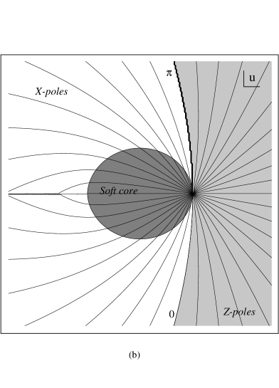
Figure 2: (a) The core and branch cut in the $Z=\phi_{D}$-plane. (b) Lines of constant $Z$-phase in the $u$-plane are shown for $\pi/20$ increments.

The $\phi_{D}$-plane is shown in figure 2(a): The closed curve is the boundary of the soft core, and the two curves running out from the bottom of the soft core are the map to the $\phi_{D}$-plane of a cut along the negative $u$-axis starting from $u=-1$. Beneath these curves are values of $\phi_{D}$ that are forbidden because of the discontinuity in $\phi_{D}$ as one crosses the cut.

Lines of constant $Z(r)$-phase in the $\phi_{D}$ plane have two types of behaviours characterized by their slopes: When the vacuum expectation value $a_{D}(u)$ lies in the upper half of the complex plane, $Z(r)$ can hit the soft quantum core region only at $u(r_{c})=1$, where $Z(r_{c})=\phi_{D}=0$, corresponding to a $Z$-pole. When $a_{D}(u)$ is in the lower half-plane, the line intersects the soft quantum core boundary at some critical radius $r_{c}$ where $X(r_{c})=0$ (and $Z(r_{c})\neq 0$), corresponding to a $X$-pole. In the latter case the solution breaks down within the soft quantum core, although one may formally continue it all the way to the $u({\tilde{r}}_{c})=1$ point where we may define the second critical radius ${\tilde{r}}_{c}$.

In the $\phi_{D}$-plane, the curves representing the branch cut tend to horizontal lines, albeit only logarithmically. Thus an $X$-pole solution has a maximum allowed value of $|Z(\infty)|$; continuing across the cut gives rise to solutions related by a monodromy transformation $M_{\infty}$ (see 5.9), and we shall find these solutions when we consider the $(n_{m},n_{e})=(1,2)$ sector. This gives an a priori independent definition of $X$-poles and $Z$-poles that is not based on boundary conditions at the core of the monopole: analytically continuing to larger mass along lines of constant $Z$-phase, $X$-poles eventually reach another charge sector. Note that for $X$-poles and $Z$-poles, the phase of $Z(r)$ (and hence of $\phi_{D}(r)$) is known from the asymptotic value; however, the explicit solution to $\phi_{D}(r)$ involves solving a nonlinear integro-differential equation for $u(r)$ (5.8). (We present an alternative formulation for the solution to $u$ through a nonlinear differential equation in Appendix A.)

In the $u$-plane, the lines of constant $Z$ phase are drawn in figure 2(b) together with the soft quantum core (shown shaded darkly). There are two types of lines corresponding to the different solutions described above. All of the lines in the $u$-plane extend outwards from the $u=1$ point. The lines in the lightly shaded region represent $Z$-poles; clearly these arise only for certain values of $u(\infty)$. The lines in the unshaded region represent $X$-poles. These eventually hit the negative $u$-axis, as described in the previous paragraph. Continuing $u$ through the negative real axis brings the solutions through the branch cut and implies a monodromy transformation; the continued solutions beyond the cut represent $X$-poles in a different charge sector.

As mentioned in section 3, the quantum corrected solutions have a remarkable feature: the $\Theta$-angle is spatially dependent! For $Z$-poles, it bleaches out as we approach the core, whereas for $X$-poles, it can either bleach or intensify depending on the value of $u(\infty)$. This may be seen simply by noting that the solutions as a function of ${\vec{r}}$ come out of the $u=1$ point to some vacuum value $u(\infty)$. The coupling constant $\tau(u)$ must change along the solution for $u({\vec{r}})$ as a function of ${\vec{r}}$. Recall that the $\Theta$-angle is determined by ${{\cal{R}}}e\left(\tau\right)$. This phenomenon has no analog classically, as the classical $\Theta$-angle is a fixed parameter. However, it is known to occur quantum-mechanically in the presence of light charged fermions. A possible interpretation of the phenomenon is that near the quantum core, the “local” mass of the $(n_{m},n_{e})=(1,0)$ dyons is going to zero, and hence the dyons themselves might act as the light fermions that bleach the $\Theta$-angle.

Figure 3: Lines of constant $Z(r)$-phase in the $\tau$-plane in the $n_{e}=0$ sector.

We illustrate the bleaching phenomenon by displaying several monopole solutions in the $\tau$-plane in figure 3. The origin corresponds to $u=1$ and the points $\pm 1$ correspond to $u=-1$. The two lower half circles in the $\tau$-plane are the map of the real line segment $u\in[-1,1]$ (the boundary of the hard core) and the two above them come from the map of the ${\cal I}m\Bigl{(}a_{D}/a\Bigr{)}=0$ curve (the boundary of the soft core) into the $\tau$-plane [15]. Several soliton solutions (i.e., lines of constant $Z(r)$ phase) in the $\tau$-plane are displayed. One sees clearly that the $\Theta$-angle changes along the lines. The $Z$-pole and $X$-pole are distinguished in this plot as usual by whether or not their solutions cross through the curve of marginal stability ${\cal I}m\Bigl{(}a_{D}/a\Bigr{)}=0$.

         

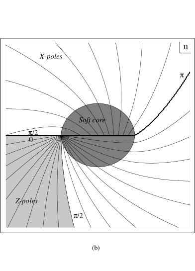
Figure 4: Sample solutions in $n_{e}=-1$ sector. Lines of constant $Z$-phase in the $u$-plane are shown for $\pi/20$ increments.

In the $n_{e}=-1$ sector the structure of the solutions is the same and is again found by following radial lines in the $Z$-plane; however, in this case the $Z(r_{c})=0$ condition appears at the $u(r_{c})=-1$ point. Sample solutions in the $Z$, $u$, and $\tau$ planes are illustrated in figures 4 and 5. Further examples for $n_{e}=2$ are given in figure 6; note that in this charge sector, all solutions are $X$-poles.

Figure 5: Lines of constant $Z(r)$-phase in the $\tau$-plane in the $n_{e}=-1$ sector.

The remaining issue to be discussed is the effect of monodromies in $a(u)$ and $a_{D}(u)$ on the quantum corrected solutions. Because of the breakdown of the BPS bound within the quantum core our analysis is restricted to the semi-classical monodromy: encircling one of the two points $u=\pm 1$ involves passing through the quantum core, about which we are ignorant. The semi-classical monodromy on the solutions is obtained from $M_{\infty}$ in (5.9).

         

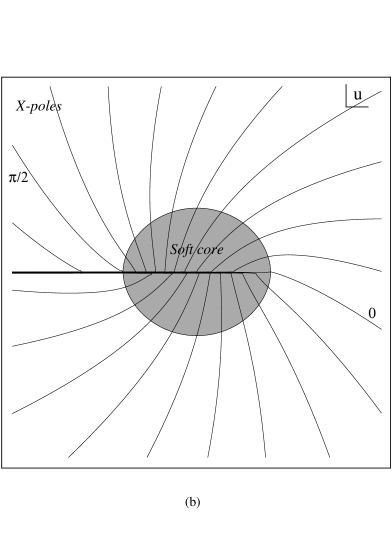
Figure 6: Sample solutions in $n_{e}=2$ sector. Lines of constant $Z$-phase in the $u$-plane are shown for $\pi/20$ increments.

We may consider a solution for some asymptotic $u(\infty)$, e.g., in the $Z$-pole region. Continuing $u(\infty)$ clockwise, the solution becomes an $X$-pole, and eventually $u(\infty)$ reaches the negative ${\cal{R}}{e}(u)$-axis. We then leave the $n_{e}=0$ sector and cross over to the $n_{e}=2$ sector; indeed, we see that the phase $-9\pi/20$ contour in figure 2(b) continues as the phase $11\pi/20$ contour in figure 6(b) (the $\pi$-phase difference is due to the change of sign of $n_{m}$ in (5.12)).

8 Spatial dependence

The general solution in (4.6) depends on a parameter $\delta$ which is presumably fixed by the microscopic theory in the quantum core region. Classically, regularity of the fields at the origin imposes $\delta=0$. We comment here on some of the effects of the $\delta$ parameter on the soliton solutions within the semi-classical region. For simplicity, we only consider the $n_{e}=0$ sector.

Asymptotically, at large $r$ the scalar field $X$ behaves as

$$\sqrt{2}X(r)=\kappa-{1\over r}+2\kappa e^{-2\kappa(r+\delta)}+\ldots\ .$$ (8.1)

The first two terms describe just the vacuum expectation value of the scalar field and the topological magnetic charge. The exponential correction reflects the presence of the massive vector bosons in the theory; the decay constant $\kappa=\sqrt{2}{{\cal{R}}}e\left(\exp(i\alpha)a\right)$ is proportional to their mass ($\sqrt{2}|a|$). The $\delta$ parameter does not affect the rate of fall-off; rather, it suppresses the exponential correction by a factor $e^{-2\kappa\delta}$. Physically, this suggests that $\delta$ reflects the absence of the massive vector bosons in the quantum core, and a resulting suppression of their contribution to the monopole. Indeed, taking $\delta\to\infty$ leads to a Coulomb form for the magnetic and electric fields in (4.2).

The critical radius $r_{c}$ for $X$-poles is determined by the condition $X(r_{c})=0$:

$$\sqrt{2}X(r_{c})=\kappa\coth{\kappa(r_{c}+\delta)}-{1\over r_{c}}=0\ .$$ (8.2)

This implies that for $X$-poles, $r_{c}$ is always less than the classical core radius $R\equiv 1/\kappa$ for any $\delta$, with $r_{c}\to 0$ when $\delta\to 0$ and $r_{c}\to R$ when $\delta\to\infty$. Note that as $X(\infty)$ tends to the curve of marginal stability, the classical radius $R=1/(\sqrt{2}X(\infty))$ as well as $r_{c}$ tend to $\infty$.

For $Z$-poles in the $n_{e}=0$ sector, $Z(r_{c})=0$ implies

$$\sqrt{2}X(r_{c})=\kappa\coth{\kappa(r_{c}+\delta)}-{1\over r_{c}}=\sqrt{2}{{\cal{R}}}e\Bigl{[}e^{i\alpha}\phi(u=1)\Bigr{]}=\frac{4\sqrt{2}}{\pi}\cos{\alpha}\ ,$$ (8.3)

where $\cos{\alpha}=\sin{\left(arg(Z)\right)}$, and is always positive, as $n_{e}=0$ $Z$-poles occur when $a_{D}$ is in the upper half-plane (see figure 2a). The value $\phi(u=1)=4/\pi$ is an instanton induced constant that is proportional to $\Lambda$ (we have set $\Lambda=1$ throughout the paper). In the limit of vanishing $\Lambda$, $r_{c}\to 0$, and the monopole becomes classical.

Figure 7: The ratio $r_{c}/R$ as a function of $R$ for $\delta=\{.01,.022,.035,\infty\}$ and $\alpha=0$.

Whereas for $X$-poles $r_{c}\leq R$, for $Z$-poles, the quantum core radius $r_{c}$ may be less than or greater than the classical core radius $R$, depending on the values of $R$, $\delta$ and $\alpha$. In figure (7), the $r_{c}/R$ is plotted against $R$ for various values of $\delta$, with $\alpha=0$. For $Z$-poles, as $u(\infty)\to 1$, the classical radius $R=1/(\sqrt{2}X(\infty))$ remains finite whereas the quantum radius $r_{c}\to\infty$. For $Z$-poles with $n_{e}=\pm 1$, the situation is very similar, with $\cos\alpha\to\pm\sin\alpha$ above, and the phase of $Z$ is restricted to the quadrant that ensures ${\cal{R}}{e}(\exp(i\alpha)\phi(r_{c}))=\lim_{\varepsilon\to 0}{\cal{R}}{e}(\exp(i\alpha)\phi(u=-1\pm\varepsilon))$ is positive (see figure 4(a) for $n_{e}=-1$; the analogous figure for $n_{e}=1$ is simply the reflection about the ${\cal{I}}{m}(Z)$-axis).

9 Next Order Corrections

In the low-energy theory described by the superpotential ${\cal F}(\phi)$ we have shown how BPS saturated states arise and generalize the classical soliton solutions. However, the superpotential ${\cal F}(\phi)$ is just the first term in a momentum expansion of the low-energy effective action. There are higher derivative corrections; the first term is a real potential ${\cal H}$ of dimension zero integrated over the full $N=2$ superspace measure (2.3). In this section we find how these higher order corrections affect the quantum solitons. Contributions to ${\cal H}$ of two different kinds have been discussed [3, 4, 17, 20].

In [4] it was found that the one-loop correction to the Kähler potential associated to the nonabelian low-energy theory $L_{\cal F}$ cannot be written in the form ${{\cal{I}}}m{\bar{\phi}}{\cal F}_{\phi}$ unless $\phi$ and $\bar{\phi}$ commute. This is in direct conflict with the constraints imposed by special geometry. However, the next order correction ${\cal H}(W,{\bar{W}})$ discussed in [4] contributes to the nonabelian part of the low-energy theory and repairs the apparent inconsistency. Here, we focus on this particular contribution, as it gives rise to corrections to the Kähler potential (albeit, corrections that vanish in the abelian limit).

The correction ${\cal H}$ we take is a function of the parameter

$$t={\phi\cdot{\bar{\phi}}\over\sqrt{\phi^{2}{\bar{\phi}}^{2}}}\ .$$ (9.1)

The parameter $t=1$ when the fields are restricted to be abelian. All scalar derivative terms of the ${\cal H}$ contribution when written as a function of $t$ are given in appendix B.

In addition to the nonabelian correction above, an explicit form for the abelian correction has been proposed in [20]:

$${\cal H}(\phi,{\bar{\phi}})=4\pi^{2}|\frac{\partial\phi}{\partial u}|^{4}|u^{2}-1|({{\cal{I}}}m\tau)^{2}\ .$$ (9.2)

This term is expressed as a function of the dimensionless group invariant $x=\phi^{2}/\Lambda^{2}$, in contrast to the parameter $t$ in (9.1). As a result, the scalar derivatives of ${\cal H}$ in this form will be quite different. For example, whereas the ${\cal H}_{A}$ term vanishes for the nonabelian correction when expressed as a function of $t$, it contributes to the full $U(1)$ term. Higher derivatives are also different, and in some sense the two corrections are orthogonal to one another. We have not investigated the contribution of this term to the dyon mass.

The contribution from the ${\cal H}$ function in (2.3) to the Lagrangian when expanded out into $N=0$ components contains many higher derivative terms, and we refer to appendix B for the explicit calculation. Previously we found the canonical Hamiltonian associated to the superpotential ${\cal F}$; because of the higher derivative terms, it is awkward to define the Hamiltonian canonically. Rather, we evaluate the time-like components of the energy-momentum tensor derived from the full Lagrangian. A general term $S_{i}$ in the action with $n$ indices may be written as

$$S_{i}=\int d^{4}x\sqrt{-g}g^{{\underline{a}}_{1}{\underline{b}}_{1}}\ldots g^{{\underline{a}}_{n}{\underline{b}}_{n}}T_{{\underline{a}}_{1}{\underline{b}}_{1}}\ldots\mbox{}_{{\underline{a}}_{n}{\underline{b}}_{n}}$$ (9.3)

where we take a mostly positive Minkowski metric. By varying with respect to the metric and looking at the 00-components we find the energy contribution from this term as

$$E=\frac{1}{2}T_{i_{1}i_{1}}\ldots\mbox{}_{i_{n}i_{n}}+\frac{1}{2}\left(T_{00\;i_{2}i_{2}}\ldots\mbox{}_{i_{n}i_{n}}+{\rm perms}.\right)-\frac{3}{2}\left(T_{00\;00\;i_{3}i_{3}}\ldots\mbox{}_{i_{n}i_{n}}+{\rm perms}.\right)+\ldots$$ (9.4)

Terms with $\epsilon$ tensors must be treated differently since they transform as densities. All of these contributions vanish when $\phi$ is real; the electric field is vanishing in this case and no nonzero contractions of the field strength and its dual are possible.

For simplicity we only consider radially symmetric soliton backgrounds and we investigate their contribution to the energy. The gauge and scalar fields in the radial ansatz are given in (4.1), and we find the contribution to the energy of the soliton by substituting their form into the expansion of the energy as derived from ${\cal H}$. In the radial ansatz the parameter $t\equiv 1$ throughout all space, and the net contribution is expressed in terms of the two constants ${\cal H}^{\prime}$ and ${\cal H}^{\prime\prime}$ presumably determined by the nonperturbative structure of the low-energy theory. Details of the full calculation from all the terms in the $N=2$ superspace expansion are given in appendix B.

The contribution from ${\cal H}(W,{\bar{W}})$ to the energy of the radially symmetric field configuration is given below. For ease of reading we group the terms into four contributions:

$$E_{1} = 2\pi(2{\cal H}^{\prime\prime}+{\cal H}^{\prime})\int dr~{}\frac{1}{\bigl{|}\phi^{4}\bigr{|}}\left(\frac{L^{2}}{r}\right)^{2}\Bigl{\{}\left(\bigl{|}\phi\bigr{|}^{2}+\frac{1}{2}b^{2}-\frac{1}{2}\left(\frac{L_{r}}{L}\right)^{2}\right)^{2}-b^{4}\Bigr{\}}\ ,$$

$$E_{2} = \pi{\cal H}^{\prime}\int dr~{}{1\over|\phi|^{2}}|L_{r}{\phi_{r}\over\phi}+{L(1-L^{2})\over r^{2}}|^{2}-{L^{2}b^{2}\over|\phi|^{2}}|{b_{r}\over b}-{\phi_{r}\over\phi}|^{2}\ ,$$

$$E_{3} = 4\pi{\cal H}^{\prime}\int dr~{}\left(\frac{Lr}{2}-\frac{gr^{2}}{4\phi\bar{\phi}}\right)\left\{2\frac{L(1-L^{2})}{r^{3}}+\frac{L_{r}}{r}\left(\frac{\phi_{r}}{\phi}+c.c.\right)\right\}\ ,$$ (9.5)

$$E_{4} = 4\pi{\cal H}^{\prime}\int dr~{}\frac{r^{2}}{\bigl{|}\phi\bigr{|}^{2}}\left\{\left(\frac{g}{2}-\frac{L\bigl{|}\phi\bigr{|}^{2}}{r}\right)^{2}-\left(\frac{b^{2}L}{r}\right)^{2}\right\}\ .$$

In equation (9) the function $g$ is defined by

$$g\equiv\frac{L_{rr}}{r}+\frac{L(1-L^{2})}{r^{3}}-\frac{Lb^{2}}{r}\ ,$$ (9.6)

and arises naturally in the covariant derivative of the field strength in the radial ansatz.

We find by inserting the quantum dyon solution for the fields $L(r)$, $\phi(r)$, and $b(r)$ in (4.6) and (4.3) into the energy expression above that both the ${\cal H}^{\prime}$ and ${\cal H}^{\prime\prime}$ terms are individually vanishing. Remarkably, the classical monopole and dyon appears generically in the low-energy effective $N=2$ theory – including the next order corrections. The BPS mass formula does not receive further corrections from these terms. Although it seems astonishing that corrections to the gauge-field kinetic terms [4] do not change soliton masses, this is an expected consequence of supersymmetry.

10 Discussion

We believe that our attempt to understand quantum corrections to solitons by studying minima of the quantum corrected low-energy effective Hamiltonian opens up a new area for investigation. We conclude with a list of open problems.

We would like to understand what happens inside the quantum core and to determine the unknown parameter $\delta$. For $Z$-poles, there seems to be a promising approach: near $u=1$, there is a dual description in terms of a fundamental monopole hypermultiplet weakly coupled to the dual $U(1)$ gauge-supermultiplet $W_{D}$ (whose leading scalar component is $\phi_{D}$). Unfortunately, this dual description is infrared free, so when the quantum core is small, the theory cannot be considered weakly coupled. It remains to be seen if there is a range of parameters where a useful description can be found.

It is also interesting to investigate multi-monopole configurations. Although one cannot use the radial ansatz, we believe that much of our analysis would survive, and in particular, that the phase of the local central charge $Z(\vec{r})$ would be constant everywhere in space. In classical multi-pole configurations, there are multiple zeros of $\phi$; correspondingly, we expect that the quantum-corrected multi-poles should have multiple quantum cores.

The low-energy dynamics of a charge $k$ monopole in a classical $SU(2)$ Yang-Mills-Higgs theory broken to $U(1)$ is modelled by geodesic motion on a smooth $4k$-dimensional hyperkähler manifold [21]. Presumably, quantum moduli spaces also inherit the hyperkähler property from the BPS equations, and an $SO(3)$ group of isometries from spatial rotations of the monopoles. For well separated monopoles (where the vacuum expectation values are such that the quantum cores are sufficiently small), we expect the metric to be smooth and very similar to the classical case. In this limit the exponential corrections to the classical monopole and moduli spaces are negligible, and the hyperkähler metric models the motion of point-like monopoles. However, to understand the quantum moduli spaces fully, we need to find the effects of the quantum cores; in particular, do they spoil the completeness of the moduli spaces or change the topology near the origin?

In particular, for the classical charge two configuration, two incoming monopoles may be converted into outgoing electrically charged dyons [22, 21]. In the quantum theory, monodromies can change the charges of monopoles. It would be interesting to see if there is a relation between these facts: How do quantum effects modify the charge exchange process, and are monodromies involved?

Beyond answering questions about the pure $SU(2)$ theory, it is interesting to consider a variety of extensions: One can add fundamental hypermuliplets, or go to higher rank gauge groups. Indeed, the simplest quantum moduli space to investigate describes distinct fundamental monopoles in higher-rank gauge groups. In this case, the the moduli space in the classical theory is the higher dimensional analog of the Taub-NUT metric [23, 24, 25] and has neither exponential corrections nor charge exchange scattering. This suppression is caused by the existence of a maximal number of commuting triholomorphic isometries on the moduli space, a feature that should persist in the quantum theory.

In the low-energy $N=2$ effective action for higher rank gauge groups, the gauge symmetry is always broken down to its maximal torus. Recently, it has been shown that in the classical theory with nonminimal gauge breaking there are monopole configurations which lead to a new interpretation of some of the $4k$ coordinates parameterizing its moduli space [26]; in these particular examples there are nonabelian fields present and some parameters measure the orientation and “cloud” size of the nonabelian fields. Since the low-energy effective $N=2$ theory does not have enhanced gauge symmetry, these configurations should be suppressed by instanton effects; our results may shed light on this phenomenon.

Recently, the dimensional reduction of $N=2$ super gauge theories to $N=4$ supersymmetric gauge theories in $d=2+1$ dimensions has been investigated in both field theory and string theory [27, 28, 29, 30]. In this case the (reduced) moduli space of charge $k$ monopoles is isomorphic to the quantum corrected Coulomb branch of $SU(k)$ gauge theories. From the gauge theory point of view, the exponential corrections to the multi-monopole moduli space metric are obtained through three-dimensional instanton effects. It would be interesting to see if our results have any implications in this context.

Finally, a potentially interesting extension of our work comes from embedding $N=2$ super Yang-Mills theories in string theories and studying the relation of monopoles to D-branes; to date, such studies have not focused on the explicit form of quantum corrected stringy solitons. Extensions of our work to this context might prove illuminating both for field theory and for string theory.

Acknowledgements

We thank Martin Bucher, Alfred Goldhaber, Amihay Hanany, Hans Hansson, Ismail Zahed, Philip Argyres, Kimyeong Lee, and Piljin Yi for discussions. The work of MR and GC was supported in part by NSF grant No. PHY 9309888.

Appendix A Differential Equation for $u(r)$

The soliton solutions as derived from the full low-energy theory are described by the complex function on the order parameter $u(r)$ through the relations on the period integrals (5.8). This gives a complicated transcendental relation between the solitons in $\phi$ space and in $u$-space. Alternatively one may derive a direct nonlinear differential equation for $u(r)$.

We consider spherically symmetric dyon configurations of $\phi_{D}$ and $\phi$. We first re-express the field equations using the Picard-Fuchs equations [11]. For any number of hypermultiplets in the theory, the periods $a(u)$ and $a_{D}(u)$ satisfy

$$p(u){d^{2}a(u)\over du^{2}}=-a(u),\quad\quad p(u){d^{2}a_{D}(u)\over du^{2}}=-a_{D}(u)\ .$$ (A.1)

The polynomial $p(u)$ depends in general on $N_{f}$; for $N_{f}=0$ it is determined to be $p(u)=4(u^{2}-1)$. Using the spherical ansatz and the Picard-Fuchs equations, the field equation for the dual scalar (3.15) may be expressed as

$${{\cal{R}}}e~{}e^{i\alpha}\Bigl{\{}\partial_{u}\phi_{D}(r^{2}u_{r})_{r}-\phi_{D}\bigl{[}{(ru_{r})^{2}\over p(u)}+2L^{2}\bigr{]}\Bigr{\}}=0\ ,$$ (A.2)

with the same equation for $\phi(u)$.

More explicitly, we can substitute the form of $\phi(u)$ and $\phi_{D}(u)$ in terms of complete elliptic integrals given in (5.4) to obtain the differential equation

$${{\cal{R}}}e~{}{e^{i\alpha}\over(1+u)^{1/2}}\Bigl{\{}K(q)(r^{2}u_{r})_{r}-2(1+u)E(q)\bigl{[}{(ru_{r})^{2}\over p(u)}+2L^{2}\bigr{]}\Bigr{\}}=0\ .$$ (A.3)

The dual scalar field equation is found by substituting (5.5) into (A.2) to obtain

$${{\cal{R}}}e~{}{ie^{i\alpha}\over(1+u)^{1/2}}\Biggl{\{}\Bigl{(}2E(q^{\prime})-K(q^{\prime})\Bigr{)}(r^{2}u_{r})_{r}-2(1+u)\Bigl{(}E(q^{\prime})-K(q^{\prime})\Bigr{)}\bigl{[}{(ru_{r})^{2}\over p(u)}+2L^{2}\bigr{]}\Biggr{\}}=0\ .$$ (A.4)

The forms (A.3) and (A.2) give two nonlinear differential equations that determine the complex order parameter $u(r)$.

Appendix B ${\cal H}$ Function Expansion

In this appendix we expand out the contribution from the bosonic portion of $S_{\cal H}$ in (2) in terms of $N=0$ components. We drop the auxilliary fields and group the terms into the following ten pieces :

$$T_{1} = {1\over 4}{\cal H}_{AB\bar{C}\bar{D}}\nabla^{{\underline{a}}}\phi^{A}\nabla_{{\underline{a}}}\phi^{B}\nabla^{{\underline{b}}}\bar{\phi}^{C}\nabla_{{\underline{b}}}\bar{\phi}^{D}+\left({1\over 4}{\cal H}_{A\bar{B}\bar{C}}\nabla^{{\underline{a}}}\nabla_{{\underline{a}}}\phi^{A}\nabla^{{\underline{b}}}\bar{\phi}^{B}\nabla_{{\underline{b}}}\bar{\phi}^{C}+c.c.\right)$$

$$+{1\over 4}{\cal H}_{A\bar{B}}\nabla^{{\underline{a}}}\nabla_{{\underline{a}}}\phi^{A}\nabla^{{\underline{b}}}\nabla_{{\underline{b}}}\bar{\phi}^{B}+{i\over 4}{\cal H}_{A\bar{B}}\nabla^{\alpha{\dot{\alpha}}}\phi^{A}\left[\nabla_{{\dot{\alpha}}}^{\beta}f_{\alpha\beta}+\nabla_{\alpha}^{{\dot{\beta}}}f_{{\dot{\alpha}}{\dot{\beta}}},\bar{\phi}\right]^{B}$$

$$T_{2} = -{\cal H}_{A{\bar{B}}}f_{CD}^{A}(\nabla^{\alpha{\dot{\beta}}}f_{\dot{\beta}}^{\dot{\alpha}})^{B}\phi^{C}\nabla_{\alpha{\dot{\alpha}}}{\bar{\phi}}^{D}+{\cal H}_{A{\bar{B}}{\bar{E}}}f_{CD}^{A}\nabla^{\alpha{\dot{\beta}}}{\bar{\phi}}^{E}(f_{\dot{\beta}}^{\dot{\alpha}})^{B}\phi\nabla_{\alpha{\dot{\alpha}}}{\bar{\phi}}^{D}+{\rm c.c.}$$ (B.1)

$$T_{3} = -{1\over 4}{\cal H}_{{\bar{A}}CD}\nabla_{{\underline{a}}}\nabla^{{\underline{a}}}\phi^{A}(f^{\alpha\beta})^{C}(f_{\alpha\beta})^{D}+{\rm c.c.}$$ (B.2)

$$T_{4} = {\cal H}_{{\bar{A}}{\bar{B}}CD}\nabla^{\beta{\dot{\beta}}}{\bar{\phi}}^{A}(f_{\dot{\beta}}^{\dot{\alpha}})^{B}\nabla_{\dot{\alpha}}^{\alpha}\phi^{C}(f_{\alpha\beta})^{D}$$ (B.3)

$$T_{5} = {1\over 4}{\cal H}_{A{\bar{B}}}\nabla_{{\underline{a}}}\nabla^{{\underline{a}}}\phi^{A}\nabla_{{\underline{b}}}\nabla^{{\underline{b}}}{\bar{\phi}}^{B}$$ (B.4)

$$T_{6} = -{1\over 2}f_{AD}^{C}{\cal H}_{C{\bar{B}}}\phi^{D}\nabla^{\beta{\dot{\alpha}}}{\bar{\phi}}^{B}(\nabla_{\beta}^{\dot{\beta}}f_{{\dot{\beta}}{\dot{\alpha}}})^{A}$$ (B.5)

$$T_{7} = f_{BC}^{A}f_{AE}^{G}{\cal H}_{G{\bar{D}}}\phi^{E}\nabla^{{\underline{a}}}{\bar{\phi}}^{D}\phi^{B}\nabla_{{\underline{a}}}{\bar{\phi}}^{C}$$ (B.6)

$$T_{8} = {\cal H}_{A{\bar{B}}}(\nabla^{\beta{\dot{\alpha}}}f_{\beta}^{\alpha})^{B}(\nabla_{\alpha}^{\dot{\mu}}f_{{\dot{\mu}}{\dot{\alpha}}})^{A}$$ (B.7)

$$T_{9} = {1\over 4}{\cal H}_{A{\bar{B}}C{\bar{D}}}(f^{\alpha\beta})^{A}(f_{\alpha\beta})^{C}(f^{{\dot{\alpha}}{\dot{\beta}}})^{B}(f_{{\dot{\alpha}}{\dot{\beta}}})^{D}$$ (B.8)

$$T_{10} = {\cal H}_{{\bar{B}}CD}(\nabla^{\beta{\dot{\beta}}}f_{\dot{\beta}}^{\dot{\alpha}})^{B}\nabla_{\dot{\alpha}}^{\alpha}\phi^{C}(f_{\alpha\beta})^{D}+c.c.$$ (B.9)

The energy associated to the above terms may be derived from the 00-component of the energy momentum tensor. We insert the explicit metric tensor in each term as in (9.3) and then vary with respect to them. The general term in the action contributes an energy as listed in (9.4). We note, however, that it is important to track the explicit $\epsilon$ tensors arising in the bosonic form of ${\cal H}$ since they transform as tensor densities and thus come with different powers of $\sqrt{-g}$ when compared with terms only containing the metric. Such terms are absent in the case of vanishing electric field however, because all covariant time derivatives of the Higgs field are zero.

As is clear in (B-B.9) the complete expression for $E$ contains derivatives of ${\cal H}(t)$ with respect to $\phi^{A}$ or $\bar{\phi}^{A}$. The potential ${\cal H}$ is only a function of $t=\frac{\phi\cdot\bar{\phi}}{\sqrt{\phi^{2}\bar{\phi}^{2}}}$, so that we may find simple expressions for the derivatives. It is convenient to express them in terms of the projection operator ${\Pi}_{AB}=\delta_{AB}-e_{A}e_{B}$ on the coset $SU(2)/U(1)$, introduced in (6.3), and the unit vector $e^{A}\equiv\langle\phi^{A}/\sqrt{\phi^{2}}\rangle$. There are only two generic parameters ${d\over dt}{\cal H}(t)={\cal H}^{\prime}$ and ${\cal H}^{\prime\prime}$ which in the spherical ansatz are evaluated at $t=1$. We give the explicit form of the scalar derivatives on ${\cal H}$ below:

$${\cal H}_{A} \equiv \frac{\partial{\cal H}}{\partial\phi^{A}}=0$$

$${\cal H}_{A\bar{B}} = \frac{{\cal H}^{\prime}}{\phi\bar{\phi}}{\Pi}_{AB}$$

$${\cal H}_{AB\bar{C}} = -\frac{{\cal H}^{\prime}}{\phi^{2}\bar{\phi}}\left({\Pi}_{AC}e_{B}+{\Pi}_{BC}e_{A}\right)$$ (B.10)

$${\cal H}_{AB\bar{C}\bar{D}} = \frac{{\cal H}^{\prime\prime}}{\phi^{2}\bar{\phi}^{2}}\left({\Pi}_{AB}{\Pi}_{CD}+{\Pi}_{AC}{\Pi}_{BD}+\Pi_{AD}{\Pi}_{BC}\right)$$

$$+\frac{{\cal H}^{\prime}}{\phi^{2}\bar{\phi}^{2}}\left({\Pi}_{AB}{\Pi}_{CD}+{\Pi}_{AC}e_{B}e_{D}+{\Pi}_{AD}e_{B}e_{C}+\Pi_{BC}e_{A}e_{D}+{\Pi}_{BD}e_{A}e_{C}\right)$$

Within the radial ansatz the field strengths decompose in a simple manner onto the $U(1)$ and $SU(2)/U(1)$ directions. We use the following conventions

$$F_{\mu\nu}^{A} = \partial_{\mu}A_{\nu}^{A}-\partial_{\nu}A_{\mu}^{A}+\epsilon^{A}_{~{}BC}A_{\mu}^{B}A_{\nu}^{C}\ .$$ (B.11)

The electric and magnetic fields, together with the covariant derivative on the scalar, are explicitly

$$E_{i,A} = -b_{r}e_{i}e_{A}-{bL\over r}{\Pi}_{iA}$$ (B.12)

$$B_{i,A} = -{(1-L^{2})\over r^{2}}e_{i}e_{A}+{L_{r}\over r}{\Pi}_{iA}$$ (B.13)

$$\nabla_{i}\phi_{A} = \phi_{r}e_{i}e_{A}+{L\phi\over r}{\Pi}_{iA}\ .$$ (B.14)

Further covariant derivatives of the field strength are not listed.

The computation of the energy $E$ using the derivatives of $H$ in (B) and the fields (B.12) is straightforward but intensive. We first list terms that are proportional to the constant ${\cal H}^{\prime\prime}(1)$. The index $i$ in $E_{i}$ below refers to the term in (B-B.9) in which it arises:

$$E_{1}^{\prime\prime} = {\cal H}^{\prime\prime}\left(\frac{L}{r}\right)^{4}$$ (B.15)

$$E_{4}^{\prime\prime} = {\cal H}^{\prime\prime}\frac{1}{\phi\bar{\phi}}\left(\frac{L}{r}\right)^{2}\left(\left(\frac{bL}{r}\right)^{2}-\left(\frac{L_{r}}{r}\right)^{2}\right)$$ (B.16)

$$E_{9}^{\prime\prime} = {\cal H}^{\prime\prime}\frac{1}{4\phi^{2}\bar{\phi}^{2}}\left(\left(\frac{L_{r}}{r}\right)^{2}-\left(\frac{bL}{r}\right)^{2}\right)^{2}-{\cal H}^{\prime\prime}\frac{1}{\phi^{2}\bar{\phi}^{2}}\left(\frac{bL}{r}\right)^{4}$$ (B.17)

The net contribution proportional to ${\cal H}^{\prime\prime}(1)$ may then be simplified to

$$E^{\prime\prime}={\cal H}^{\prime\prime}\frac{1}{\bigl{|}\phi\bigr{|}^{4}}\left(\frac{L}{r}\right)^{4}\left\{\left(\bigl{|}\phi\bigr{|}^{2}+\frac{1}{2}\left(b^{2}-\left(\frac{L_{r}}{L}\right)^{2}\right)\right)^{2}-b^{4}\right\}\ .$$ (B.18)

The remaining contributing terms to $E$ are proportional to ${\cal H}^{\prime}$. We suppress the constant ${\cal H}^{\prime}$ and list them below:

$$E_{1}^{\prime} = \frac{1}{4}\left\{\frac{L^{2}(1+L^{2})}{r^{4}}-\left(\frac{L_{r}}{r}\right)^{2}-\left(\frac{Lb}{r}\right)^{2}\right\}$$ (B.19)

$$E_{2}^{\prime} = \left(\frac{L_{r}}{r}\right)^{2}+\left(\frac{bL}{r}\right)^{2}+\frac{LL_{r}}{2r^{2}}\left(\frac{\phi_{r}}{\phi}+\frac{\bar{\phi}_{r}}{\bar{\phi}}\right)$$ (B.20)

$$E_{4}^{\prime} = \frac{1}{4\phi\bar{\phi}}\left\{\left(\frac{L}{r}\right)^{2}\left[\frac{(1-L^{2})^{2}}{r^{4}}-2\left(\frac{L_{r}}{r}\right)^{2}+2\left(\frac{bL}{r}\right)^{2}-b_{r}^{2}\right]\right.$$ (B.21)

$$\left.+\Bigl{|}\frac{\phi_{r}}{\phi}\Bigr{|}^{2}\left(\left(\frac{L_{r}}{r}\right)^{2}-\left(\frac{bL}{r}\right)^{2}\right)\right.$$

$$\left.+\left(\frac{L_{r}L(1-L^{2})}{r^{4}}+bb_{r}\left(\frac{L}{r}\right)^{2}\right)\left(\frac{\phi_{r}}{\phi}+\frac{\bar{\phi}_{r}}{\bar{\phi}}\right)\right\}$$

$$E_{6}^{\prime} = -\frac{Lg}{4r}$$ (B.22)

$$E_{7}^{\prime} = \frac{L^{2}\phi\bar{\phi}}{r^{2}}$$ (B.23)

$$E_{8}^{\prime} = \frac{g^{2}}{4\phi\bar{\phi}}-\frac{1}{\phi\bar{\phi}}\left(\frac{b^{2}L}{r}\right)^{2}$$ (B.24)

$$E_{9}^{\prime} = \frac{1}{2}\left[\frac{L_{r}^{2}-(Lb)^{2}}{2r^{2}\phi\bar{\phi}}\right]^{2}-\frac{1}{2}\left(\frac{b^{2}L^{2}}{r^{2}\phi\bar{\phi}}\right)^{2}$$ (B.25)

$$E_{10}^{\prime} = -\frac{g}{4\phi\bar{\phi}}\left[2\frac{L(1-L^{2})}{r^{3}}+\frac{L_{r}}{r}\left(\frac{\phi_{r}}{\phi}+\frac{\bar{\phi}_{r}}{\bar{\phi}}\right)\right]-\frac{b^{3}L^{2}}{2\phi\bar{\phi}r^{2}}i\left(\frac{\phi_{r}}{\phi}-\frac{\bar{\phi}_{r}}{\bar{\phi}}\right)\ .$$ (B.26)

We have defined the function $g(r)$ to be

$$g(r)=\frac{L_{rr}}{r}+\frac{L(1-L^{2})}{r^{3}}-\frac{Lb^{2}}{r}\ .$$ (B.27)

The net sum from (B.19) simplifies to the form

$$E_{a}^{\prime} = {\cal H}^{\prime}\frac{1}{2\bigl{|}\phi\bigr{|}^{4}}\left(\frac{L}{r}\right)^{4}\left\{\left(\bigl{|}\phi\bigr{|}^{2}+\frac{1}{2}\left(b^{2}-\left(\frac{L_{r}}{L}\right)^{2}\right)\right)^{2}-b^{4}\right\}$$ (B.28)

$$E_{b}^{\prime} = {\cal H}^{\prime}{1\over 4r^{2}|\phi|^{2}}|L_{r}{\phi_{r}\over\phi}+{L(1-L^{2})\over r^{2}}|^{2}-{\cal H}^{\prime}{L^{2}b^{2}\over 4r^{2}|\phi|^{2}}|{b_{r}\over b}-{\phi_{r}\over\phi}|^{2}$$ (B.29)

$$E_{c}^{\prime} = {\cal H}^{\prime}\left(\frac{L}{2r}-\frac{g}{4\phi\bar{\phi}}\right)\left\{2\frac{L(1-L^{2})}{r^{3}}+\frac{L_{r}}{r}\left(\frac{\phi_{r}}{\phi}+c.c.\right)\right\}$$ (B.30)

$$E_{d}^{\prime} = {\cal H}^{\prime}\frac{1}{\bigl{|}\phi\bigr{|}^{2}}\left\{\left(\frac{g}{2}-\frac{L\bigl{|}\phi\bigr{|}^{2}}{r}\right)^{2}-\left(\frac{b^{2}L}{r}\right)^{2}\right\}\ .$$ (B.31)

The energy associated to the spherically symmetric soliton arising from the real nonchiral ${\cal H}$ potential is thus given by the sum of (B.18) and (B.28-B.31).

References

- [1] N. Seiberg and E. Witten, Nucl. Phys. B431 (1994) 484, hep-th/9408099.
-
[2]
G. Sierra and P.K. Townsend, in Supersymmetry and
Supergravity 1983, proc. XIXth Winter School, Karpacz,
ed. B. Milewski (World Scientific, 1983), p. 396,
B. de Wit, P.G. Lauwers, R. Philippe, S.-Q. Su and A. Van Proeyen, Phys. Lett. B134 (1984) 37,
S.J. Gates, Nucl. Phys. B238 (1984) 349. - [3] M. Henningson, Nucl. Phys. B458 (1996) 445, hep-th/9507135.
- [4] B. de Wit, M.T. Grisaru, M. Rocek, Phys. Lett. B374 (1996) 297.
-
[5]
E.B. Bogomol’ny, Sov. J. Nucl. Phys. 24 (1976) 449,
M. K. Prasad and C. H. Sommerfield, Phys. Rev. Lett. B35 (1975) 760. - [6] B. Julia and A. Zee, Phys. Rev. D11 No.8 (1975) 2227.
- [7] E. Witten, Phys. Lett. B86 (1979) 283.
- [8] Erick J. Weinberg and Alan H. Guth, Phys. Rev. D14 (1976) 1660.
- [9] E. Weinberg, Nucl. Phys. B167 (1980) 500.
- [10] S.J. Gates, M.T. Grisaru, M. Roček and W. Siegel Superspace (Benjamin-Cummings 1983).
-
[11]
A. Klemm, W. Lerche, S. Yankielowicz, S. Theisen, Phys. Lett. B344 (1995) 169
A. Klemm, W. Lerche, S. Theisen, Int. J. Mod. Phys. A11 (1996) 1929. -
[12]
U. Lindström and M. Roček,Phys. Lett. B355 (1995) 492, hep-th/9503012,
A. Giveon and M. Roček,Phys. Lett. B363 (1995) 173, hep-th/9508043. - [13] A. Bilal, F. Ferrari, Nucl. Phys. B469 (1996) 387.
- [14] A. Fayyazuddin, Mod. Phys. Lett. A10 (1995) 492.
- [15] P.C. Argyres, A.E. Faraggi, A.D. Shapere, hep-th/9505190.
- [16] E. Witten and D. Olive, Phys. Lett. B78 (1978) 97.
- [17] U. Lindström, F. Gonzalez-Rey, M. Roček, R. von Unge, ITP-SB-96-34 Phys. Lett. B to appear, hep-th/9607089.
- [18] C. Montonen, D. Olive, Phys. Lett. B72 (1977) 117.
-
[19]
G. t’ Hooft, Nucl. Phys. B79 (1974) 276,
A. Polyakov, JETP Lett. 20 (1974) 194. - [20] M. Matone, hep-th/9610204.
- [21] M.F. Atiyah, N.J. Hitchin, “The Geometry and Dynamics of Magnetic Monopoles,” Princeton Univ. Press (1988).
- [22] M.F. Atiyah, N.J. Hitchin, Phys. Lett. 107A (1985) 21.
- [23] K. Lee, E.J. Weinberg, P. Yi, Phys. Rev. D54 (1996) 1633.
- [24] M. K. Murray, hep-th/9605054.
- [25] G. Chalmers, hep-th/9605182.
- [26] K. Lee, E.J. Weinberg, P. Yi, Phys. Rev. D54 (1996) 6351.
- [27] N. Seiberg, E. Witten, hep-th/9607163.
- [28] G. Chalmers, A. Hanany, hep-th/9608105.
- [29] D. Diaconescu, hep-th/9608163.
- [30] A. Hanany, E. Witten, hep-th/9611230.