LBNL-039707, UCB-PTH-96/58

hep-th/9612131

Mirror Symmetry in Three-Dimensional Gauge Theories, $SL(2,Z)$ and D-Brane Moduli Spaces

Jan de Boer, Kentaro Hori, Hirosi Ooguri, Yaron Oz and Zheng Yin

Department of Physics, University of California at Berkeley
366 Le Conte Hall, Berkeley, CA 94720-7300, U.S.A.
and
Theoretical Physics Group, Mail Stop 50A–5101
Ernest Orlando Lawrence Berkeley National Laboratory, Berkeley, CA 94720, U.S.A.

We construct intersecting D-brane configurations that encode the gauge groups and field content of dual $N=4$ supersymmetric gauge theories in three dimensions. The duality which exchanges the Coulomb and Higgs branches and the Fayet-Iliopoulos and mass parameters is derived from the $SL(2,Z)$ symmetry of the type IIB string. Using the D-brane configurations we construct explicitly this mirror map between the dual theories and study the instanton corrections in the D-brane worldvolume theory via open string instantons. A general procedure to obtain mirror pairs is presented and illustrated. We encounter transitions among different field theories that correspond to smooth movements in the D-brane moduli space. We discuss the relation between the duality of the gauge theories and the level-rank duality of affine Lie algebras. Examples of other dual theories are presented and explained via T-duality and extremal transitions in type II string compactifications. Finally we discuss a second way to study instanton corrections in the gauge theory, by wrapping five-branes around six-cycles in $M-$theory compactified on a Calabi-Yau 4-fold.

1 Introduction

Recently a duality between $N=4$ supersymmetric gauge theories in three dimensions has been proposed under which the Higgs and Coulomb branches and the Fayet-Iliopoulos (FI) and mass parameters are exchanged [2]. The dual gauge theories have an ALE space as Higgs branch, and were based on Kronheimer’s construction [3] of ALE spaces as a hyperkähler quotient. This duality has been generalized in [4] to gauge theories whose Higgs branch is a quiver variety. The gauge groups and field content of the gauge theories is encoded in the quiver diagrams that serve as the starting point for Kronheimer-Nakajima’s hyperkähler quotient construction of the quiver varieties [5, 6]. Various interpretations of the duality have been proposed in [7, 8, 9].

It was suggested in [8] that the duality can be interpreted as arising from the $SL(2,Z)$ symmetry of type IIB string theory. One of the aims of this paper is to apply this idea to the families of dual theories (called A and B models) introduced and analyzed in [4].

(1) The A-model has $U(k)$ gauge group, $n$ hypermultiplets in the fundamental representation of the gauge group and one hypermultiplet in the adjoint representation. Its dual B-model has $U(k)^{n}$ gauge group and matter content specified by a quiver diagram corresponding to the Hilbert scheme of $k$ points on an ALE space of $A_{n-1}$ type. By the Hilbert scheme of $k$ points on a complex surface $X$ we mean a smooth resolution of the $k$-symmetric product of $X$, $Sym^{k}X$. Concretely, there will be one hypermultiplet in the fundamental representation of one of the $U(k)$’s, and $n$ hypermultiplets charged under a pair of $U(k)$’s.

(2) The A and B models have $U(k)^{n}$ and $U(k)^{m}$ gauge groups respectively, and matter content specified by quiver diagrams corresponding to the hyperkähler quotient construction of certain moduli spaces of instantons on vector bundles over ALE spaces of $A_{n-1}$ and $A_{m-1}$ types. All matter is charged under either one or two $U(k)$ gauge groups.

The paper is organized as follows: In section 2 we associate intersecting D-brane configurations of type IIB string with the quiver diagrams and use the $SL(2,Z)$ symmetry to construct their duals and to derive the mirror map between the mass terms of the A-model and the FI terms of the B-model, in agreement with [4]. The instanton corrections to the metric on the moduli space have an important role, as discussed in [10, 4, 11]. We study them in the framework of intersecting D-brane configurations as arising from open string instantons, and find agreement with what we expect from the field theory analysis. This enables us to gain further insight into the interelation between D-brane and field theory moduli spaces. In section 3 we study the condition for complete Higgsing in the gauge theory corresponding to a general quiver diagram using D-brane configurations. We rederive results which were proposed in [4] from field theory viewpoint, and that were proven in [12]. The analysis of complete Higgsing provides a general procedure to obtain mirror pairs from quiver diagrams, which is illustrated by examples. We show that moving two 5-branes of the same type through each other is reflected as a phase transition on D3-brane worldvolume theory. We then take another point of view and discuss the gauge theory duality in relation to the level-rank duality of affine Lie algebras, which are represented on the middle homology of the moduli spaces of the gauge theories. In section 4 we consider dual Abelian gauge theories. We prove the duality using field theory methods as well as T-duality and extremal transitions in type II string compactifications. Finally, in section 5 we study once more the instanton corrections, this time by relating them to the wrappings of five-branes in $M-$theory around divisors of Calabi-Yau 4-folds, in a similar fashion as in [13].

2 Quivers and Intersecting Branes

In this section we construct configurations of intersecting three and five-branes in type IIB string theory, in such a way that the world-volume theory on the three-branes has the gauge groups and matter content associated with quiver diagrams. We will then use the $SL(2,Z)$ symmetry of type IIB string theory to study mirror symmetry and verify part of the results of [4].

Following [8] we use NS 5-branes, Dirichlet 5-branes and Dirichlet 3-branes in order to construct configurations that preserve one quarter of the space-time supersymmetry. We will use conventions and notations similar to those used in [8]: The worldvolume coordinates of the NS 5-branes, the Dirichlet 5-branes and the Dirichlet 3-branes are $(x^{0},x^{1},x^{2},x^{3},x^{4},x^{5})$, $(x^{0},x^{1},x^{2},x^{7},x^{8},x^{9})$ and $(x^{0},x^{1},x^{2},x^{6})$ respectively. The coordinate $x^{6}$, which is one of the dimensions of the worldvolume of the Dirichlet 3-branes is compactified on a circle of radius $R$. The fact that the coordinate $x^{6}$ is compactified on a circle will change the field content of the worldvolume theory compared to the cases studied in [8] where the coordinate $x^{6}$ took values on the real line.

The position of the $i$th NS 5-brane in $(x^{7},x^{8},x^{9})$ will be denoted by $\vec{\omega}_{i}$. Between the $(i-1)$th and $i$th NS 5-brane there will be $k_{i}$ 3-branes, whose world-volume theory contains a $U(k_{i})$ gauge group. The Fayet-Iliopoulos parameters $\{\vec{\zeta}_{i}\}$ for this $U(k_{i})$ gauge group are related to the parameters $\{\vec{\omega}_{i}\}$ by

$$\vec{\zeta}_{i}=\vec{\omega}_{i}-\vec{\omega}_{i-1}\mskip 6.0mu.$$ (2.1)

The position of the $i$th Dirichlet 5-brane in $(x^{3},x^{4},x^{5})$ will be denoted by $\vec{m}_{i}$ and will correspond to the mass parameter associated with the $i$th hypermultiplet in the fundamental representation. This hypermultiplet arises from an open string stretching between the $i$th Dirichlet 5-brane and the Dirichlet 3-brane. The position of the Dirichlet 3-brane in $(x^{3},x^{4},x^{5})$ will correspond to the vev’s of the scalars in the vector multiplet which together with the vev’s of the scalars dual to the vector fields on the Dirichlet 3-brane worldvolume parameterize the vector multiplet moduli space. The position of the Dirichlet 3-brane in $(x^{7},x^{8},x^{9})$ will be non-linearly related to the vev’s of the scalars in the hypermultiplets and constitute part of the coordinates on the hypermultiplet moduli space. The $x^{6}$ component of the vector field provides the remaining coordinates. The $U(1)$ isometries of the hypermultiplet moduli space correspond to gauge transformations of this component.

After compactification in the $x^{6}$-direction, the three dimensional theory on the $(x^{0},x^{1},x^{2})$ worldvolume of the Dirichlet 3-brane is an $N=4$ supersymmetric gauge theory. From now on we will refer to this three dimensions as the Dirichlet 3-brane worldvolume. The gauge coupling of the Dirichlet 3-brane worldvolume theory is determined by the separation $r$ between the NS 5-branes on the circle. In particular with one NS 5-brane we have the classical relation between the three and four dimensional coupling constants

$$\frac{1}{g^{2}_{3}}=\frac{r}{g_{4}^{2}}$$ (2.2)

where $r$ denotes, in this case, the radius of the compact $6$th direction. One expects, however, corrections to this classical formula. The R-symmetry group is $SU(2)_{L}\times SU(2)_{R}$ under which the masses and FI parameters transform as $({\bf 3,1})$ and $({\bf 1,3})$ respectively. The mass parameters deform the metric on the Coulomb branch and lift some of the Higgs branch, while the FI parameters deform the metric on the Higgs branch and lift some of the Coulomb branch. The Higgs branch is constructed as a hyperkähler quotient with an $SU(2)_{R}$ action and is not modified by quantum corrections.

Due to the $N=4$ supersymmetry the Coulomb branch is a hyperkähler manifold with an $SU(2)_{L}$ action. Its metric is corrected by loop and monopole corrections. The monopoles are instantons in three dimensions and they provide exponential corrections to the metric.

The duality between $N=4$ supersymmetric gauge theories in three dimensions exchanges the Higgs and Coulomb branches, the Fayet-Iliopoulos (FI) parameters and masses and the R-symmetry groups $SU(2)_{L}$ and $SU(2)_{R}$.

2.1 Duality for $U(k)$ Gauge Groups

Consider the intersecting D-brane configuration in figure 1a.

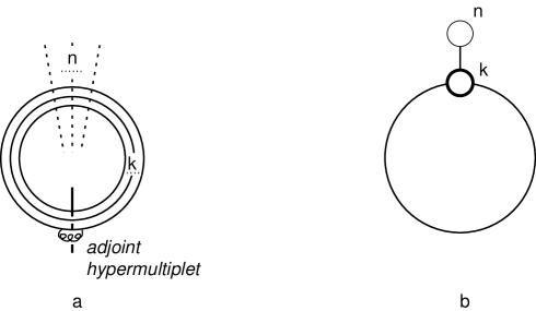
Figure 1: The D-brane configuration of the A-model is plotted on the left. The circles consist of $k$ Dirichlet 3-branes, the $n$ dashed lines are Dirichlet 5-branes and the solid line is an NS 5-brane. The corresponding quiver diagram is plotted on the right.

It consists of a NS 5-brane, $n$ Dirichlet 5-branes and $k$ Dirichlet 3-branes. In order to read off the gauge group and matter content of the three dimensional Dirichlet 3-brane worldvolume theory we have to apply the rules of [8]. When $k$ Dirichlet 3-branes end on two NS 5-branes the gauge group is $U(k)$. Since the NS 5-brane is positioned on a circle in figure 1a, the Dirichlet 3-branes do not have to end on it but can also be viewed as intersecting it and there is in addition a hypermultiplet in the adjoint representation arising from an open string connecting Dirichlet 3-branes as depicted in figure 1a. In the absence of Dirichlet 5-branes, the adjoint hypermultiplet together with the vector multiplet provide the field content for an $N=8$ supersymmetry on the world volume of the Dirichlet 3-brane, which is the reduction to three dimensions of $N=1$ super Yang Mills in ten dimensions. There are also $n$ hypermultiplets in the fundamental representation arising from the open strings connecting the $n$ Dirichlet 5-branes to the Dirichlet 3-branes.

The Dirichlet 3-branes worldvolume theory in $(x^{0},x^{1},x^{2})$ is an $N=4$ supersymmetric theory with $U(k)$ gauge group, $n$ hypermultiplets in the fundamental representation and one adjoint hypermultiplet. We will use the terminology of [4] and call this theory the A-model.

The gauge group and matter content of the A-model is associated with the quiver diagram in figure 1b, in a way which will be described below. The field content is precisely what is needed for the hyperkähler quotient construction of the moduli space of $SU(n)$ $k-$instantons $\overline{\cal M}_{k}(SU(n))$ [14], which is the Higgs branch of the theory.

We now perform an $SL(2,Z)$ transformation on the configuration of figure 1a. Recall that under this transformation an NS 5-brane is transformed into a Dirichlet 5-brane and vice versa, while the Dirichlet 3-brane is invariant. The $SL(2,Z)$ transformation of figure 1a yields the configuration of of figure 2a, and the resulting gauge theory corresponds exactly the quiver diagram of figure 2b. This will be called the B-model.

Figure 2: The D-brane configuration of the B-model is plotted on the left, and the corresponding quiver diagram is plotted on the right.

The gauge group and matter content is encoded in the quiver diagrams in the following way. Consider the quiver diagram in figure 2b, which contains figure 1a as a special case. We attach an index $k_{i}$ at each node $i$. There are $n$ nodes in the diagram with $k_{i}=k$ (indicated by thick circles) and one node (indicated by a thin circle) with index $1$. The gauge group and the field content of the theory are encoded in the diagram in the following way: We associate to each node (indicated by thick circles) $i$ with $k_{i}=k$ a gauge group $U(k)_{i}$, to each link (connecting two thick circles) ${}_{i}\!\circ\!\!-\!\!\!-\!\!\!-\!\circ_{j}$ with $k_{i}=k_{j}=k$ a hypermultiplet in the representation $({\bf k},{\bf k^{*}})$ of $U(k)_{i}\times U(k)_{j}$, and to the link (connecting a thick and a thin circle) attached to the node with index 1 a hypermultiplet in the fundamental representation of the $U(k)$ gauge group associated with the other node of the link. This is the field content needed for the hyperkähler quotient construction of the Hilbert scheme of $k$ points on an ALE space of type $A_{n-1}$, $X_{A_{n-1}}$[5, 6], which is the Higgs branch of the B-model.

It is worth noting that in fact we could get the matter content of the A-model without the use of an NS 5-brane in figure 1a. This corresponds to the absence of the extra fundamental hypermultiplet (thin circle) in the quiver diagram of the B-model in figure 2b. These theories are equivalent to the A and B models when the mass of the adjoint of the A-model and the sum of the FI parameters of the B-model are zero, which is indeed the case here as we will discuss later. In the A-model, the relative position in the $(x^{7},x^{8},x^{9})$ direction of the D3 branes with respect to the NS 5-brane corresponds in the B-model to the relative position in the $(x^{3},x^{4},x^{5})$ direction of the D3 branes with respect to the D5 brane. In other words, the parameters corresponding to the $U(1)$ part of the adjoint hypermultiplet in the A-model correspond to those of the vector multiplet of the diagonal $U(1)$ in the B-model. This is the D-brane picture of something discussed in the field theory context in [4], where the existence of a trivial $R^{4}$ in the hypermultiplet moduli space of the A-model and in the vector multiplet moduli space of the B-model has been pointed out.

Let us now recall some of the results of [4]. Consider the A-model: without mass terms, the vector multiplet moduli space is the $k$-symmetric product of an ALE space

$${\cal M}_{V}({\rm A-model},\vec{m}_{adj}=0,\vec{m}_{fund}=0)=Sym^{k}X_{A_{n-1}}\mskip 6.0mu.$$ (2.3)

It has singularities inherited from the simple singularity of $A_{n-1}$ type of the ALE space $X_{A_{n-1}}$, and also singularities coming from modding out by the action of the symmetric group. The masses for the fundamental hypermultiplets resolve the simple singularity of $X_{A_{n-1}}$. The mass of the adjoint hypermultiplets resolves the quotient singularities of the symmetric product. The other effect of the mass terms is to lift some of the flat directions of the hypermultiplet moduli space.

In the B-model, the resolution of the singularities of the hypermultiplet moduli space and the lifting of some of the flat directions for the vector multiplets are caused by turning on FI terms. The way in which the moduli spaces are resolved or lifted matches exactly with the A-model when the vector multiplet and hypermultiplet moduli spaces are exchanged, provided that the FI parameters are related to the mass parameters of the A-model in a certain way.

The mirror map between the mass parameters of the A-model and the FI parameters of the B-model takes the form [4]

$$\vec{m}_{i}=\sum_{l=0}^{i}\vec{\zeta}_{l},~{}~{}~{}~{}~{}~{}~{}~{}~{}~{}\vec{m}_{adj}=\sum_{l=0}^{n-1}\vec{\zeta}_{l}\mskip 6.0mu,$$ (2.4)

where $\vec{m}_{i}$ are the masses of the fundamental hypermultiplets, $\vec{m}_{adj}$ is the mass of the adjoint hypermultiplet and $\vec{\zeta}_{l}$ are the FI parameters. The freedom to shift the origin on the Coulomb branch of the A-model has been used to choose $\vec{m}_{n-1}=\vec{m}_{adj}$.

In the brane configuration of figure 1a, the mass of the adjoint hypermultiplet is zero since the length of the open string stretching between the Dirichlet 3-branes is zero. This corresponds in the dual theory to the case where the sum of the FI parameters is zero. It is not immediately clear how to turn on a mass for the adjoint hypermultiplet, or how to get a non-zero sum of the FI parameters in the intersecting brane configurations we consider. A possibility might be to turn on suitable string background fields, and it would be interesting to investigate this point further.

Since the $SL(2,Z)$ transformation exchanges the NS and Dirichlet 5-branes, it also exchanges $\vec{\omega}_{i}$ and $\vec{m}_{i}$. Using the relation between the FI parameters and $\vec{\omega}_{i}$ in (2.1) we get the mirror map

$$\vec{m}_{i}-\vec{m}_{i-1}=\vec{\zeta}_{i},~{}~{}~{}~{}~{}~{}~{}~{}~{}~{}i=1,...,n-1.$$ (2.5)

Equation (2.5) is equivalent to the mirror map (2.4) with $\vec{m}_{adj}=\sum_{l=0}^{n-1}\vec{\zeta}_{l}=0$.

As indicated in (2.3), when the mass of the adjoint hypermultiplet vanishes, the vector multiplet moduli space of the A-model with gauge group $U(k)$ is a $k$-symmetric product of the vector multiplet moduli space of an $U(1)$ theory. This can be read from figure 1a as follows: A vev for the diagonal components of the adjoint hypermultiplet can separate the $k$ Dirichlet 3-branes in $(x^{7},x^{8},x^{9})$, and each of them may be considered as independent. This implies that the vector multiplet moduli space which is parameterized by the vev’s of the bosons in the vector multiplet in $(x^{3},x^{4},x^{5})$ is a product of the vector multiplet moduli spaces of each brane modded by their permutation.

This scenario is expected from another string theory viewpoint. We can use D-branes to probe the space-time geometry and the background gauge fields of string theory, where enhanced gauge symmetry in the space-time theory is reflected in the D-brane world volume theory by enhanced global symmetry. Consider a type I string theory on $R^{7}\times T^{3}$. Performing a T-duality transformation on the $T^{3}$ coordinates we get the type I’ theory: type IIA with eight orientifolds and sixteen Dirichlet 6-branes and their images. The probes are $k$ Dirichlet 2-branes of the type IIA string. When the probes are near $n$ coinciding Dirichlet 6-branes, as in figure 3, the worldvolume theory of the probes is that of the A-model: The gauge group is $U(k)$ as a consequence of having $k$ probes, the adjoint hypermultiplet arises from the $D2-D2$ sector and the $n$ hypermultiplets in the fundamental arise from the $D2-D6$ sector. Their masslessness reflects the $U(n)$ space-time gauge symmetry as a global symmetry on the worldvolume of the probes.

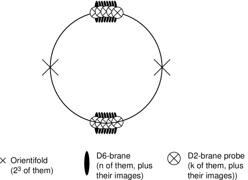
Figure 3: $k$ D2-brane probes near $n$ D6-branes in type I’

A vev for the adjoint hypermultiplet separates the Dirichlet 2-branes. The vector multiplet moduli space of each brane can be determined using the duality between M-theory on $R^{7}\times K_{3}$ and Type I string on $R^{7}\times T^{3}$ [15]. Under this duality each one of the Dirichlet 2-brane probes is mapped to an M-theory 2-brane whose world volume is $R^{3}\times\{pt\in K_{3}\}$, which implies that its vector multiplet moduli space is $K_{3}$. More precisely, the vector multiplet moduli space is determined by a neighborhood of the singularity in the $K3$ and is an ALE space of $A_{n-1}$ type. The symmetric product structure of the vector multiplet moduli space is a consequence of having $k$ separated Dirichlet 2-branes. Analogous discussion has been presented for $Sp(k)$ gauge group in [4] by taking the D2 and D6 branes to lie in an orientifold point, and for $N=2$ gauge theories in four dimensions in [16, 17].

Consider now the role of instanton corrections. When the adjoint hypermultiplet is massless we do not expect instanton corrections to the metric on the vector multiplet moduli space, while we do expect them when the adjoint is massive or absent [4]. In the following we will verify this expectation using the configurations of intersecting Dirichlet branes. This will also enable us to get an understanding of the stringy origin of the two types of coupling constants: electric and magnetic in the terminology of [8].

We expect the instanton corrections to the vector multiplet moduli space of the Dirichlet 3-brane worldvolume theory to arise from monopoles which are instantons in three dimensions. The monopoles in the D-brane picture arise from open D-string instantons stretching between the Dirichlet 3-branes [18]. Open string instantons are holomorphic maps from the disc to space-time such that the boundary of the disc is mapped to the Dirichlet brane [19, 20]. Let us begin with a qualitative analysis. In order to have open string instantons contributions in the A-model we need holomorphic maps from the disc to the cylindrical shaded area in figure 4a.

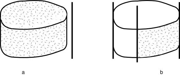
Figure 4: The image in space-time of open string instantons. There are no instanton corrections from figure 4a, but there are from figure 4b.

If we move the NS 5-brane as in figure 4a there is no such map. The reason is simple: if we think about the disc as a square then two of the edges are mapped to two Dirichlet 3-branes. The other two edges have no boundary to be mapped to. This is consistent with what we expect from field theory considerations [4]. There is a delicate point in this discussion, since if we do not move the NS 5-brane, the remaining edges can end in it. However, we do not expect to have instanton corrections in this case, as will be discussed in section 5. We therefore conclude that although the relevant holomorphic maps exist, the coefficient of the contribution is zero.

Consider now for comparison the D-brane configuration in figure 5a.

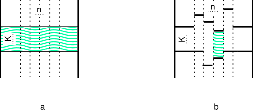
Figure 5: An $U(k)$ gauge theory with $n$ fundamentals and no adjoint hypermultiplet is plotted in its Coulomb branch on the left and in its Higgs branch on the right.

This configuration yields on the Dirichlet 3-branes a $U(k)$ gauge theory with $n$ hypermultiplets in the fundamental representation but without an adjoint. In this case a typical open string instanton is a holomorphic map from the disc to the shaded area in figure 4b, which has the topology of a disc. Such holomorphic maps exist, suggesting that we will, as expected, get instanton corrections. In section 5 we will confirm these results from a different viewpoint.

Consider now the hypermultiplet moduli space corresponding to figure 5a which is depicted in figure 5b. As we noted previously, it is determined classically and in particular is not corrected by instantons. Naively, this seems to be in contradiction with the fact that there are holomorphic maps from the disc to the shaded area in figure 5b which has the topology of a disc. Recall however that the instanton corrections are exponentials of the instanton action $\frac{|\vec{\phi}|}{g_{m}^{2}}$ where $\vec{\phi}$ corresponds to the relative position of the Dirichlet 3-brane in $(x^{7},x^{8},x^{9})$ and $\frac{1}{g_{m}^{2}}$ is the distance between the Dirichlet 5-branes [8]. The hypermultiplet moduli space is obtained in the limit $\frac{1}{g_{m}^{2}}\rightarrow 0$ which means that the shaded area in figure 5b shrinks to zero size, and therefore the instanton corrections are field independent, and should be taken into account at the classical level.

Let us now discuss the relation between open string instantons and the Dirichlet 3-brane worldvolume instantons in a more quantitative way. First recall that the four dimensional gauge coupling is related to the string coupling as

$$\frac{1}{g_{4}^{2}}=\frac{1}{g_{st}}\mskip 6.0mu,$$ (2.6)

since the coefficient of the gauge kinetic term $F^{2}$ in the open string effective action is $\frac{1}{g_{st}}$. This together with (2.2) implies that

$$\frac{1}{g_{e}^{2}}=\frac{r}{g_{st}}\mskip 6.0mu,$$ (2.7)

where by $g_{e}$ we denote the dimensionful three dimensional gauge coupling. We expect the ”magnetic” coupling to be related to the electric one (2.7) by an $SL(2,Z)$ transformation, leading to

$$\frac{1}{g_{m}^{2}}=rg_{st}\mskip 6.0mu.$$ (2.8)

In the field theory limit $r\rightarrow 0,g_{st}\rightarrow 0$ the magnetic coupling $\frac{1}{g_{m}^{2}}$ vanishes while the electric coupling $\frac{1}{g_{e}^{2}}$ can still be finite. This is the traditional field theory corner of the moduli space of D-branes.

However, the above rough analysis clearly suggests that there are other parts of the moduli space of D-branes. Consider now the open D-string instanton corrections to the vector multiplet moduli space of the 3-brane worldvolume theory. These should take the form

$$\mbox{{\rm Open D-string Instanton }}\sim\exp\left(-\frac{A}{\alpha^{\prime}g_{st}}\right)\mskip 6.0mu,$$ (2.9)

where $A$ is the area of the image of the instanton in space time. The area is $r$ times the separation between the Dirichlet 3-branes which we denote by $d$. From field theory viewpoint the instanton contribution takes the form

$$\mbox{{\rm Field Theory Instanton }}\sim\exp\left(-\frac{\langle\phi_{V}\rangle}{g_{e}^{2}}\right)\mskip 6.0mu,$$ (2.10)

where $\langle\phi_{V}\rangle$ is the vev for the scalars in the vector multiplet. This vev gives the masses of the W bosons through the Higgs mechanism. Since the masses of the W bosons, which are associated with the open strings stretching between the Dirichlet 3-branes, are given by the length of the open strings times their tension we have

$$\langle\phi_{V}\rangle=\frac{d}{\alpha^{\prime}}\mskip 6.0mu.$$ (2.11)

Using (2.11) we see that indeed (2.9) and (2.10) are the same.

Consider now the open string instantons. Their correction should take the form

$$\mbox{{\rm Open String Instanton }}\sim\exp\left(-\frac{A}{\alpha^{\prime}}\right)\mskip 6.0mu.$$ (2.12)

From a ”field theory” viewpoint the instanton contribution takes the form

$$\mbox{{\rm"Field Theory" Instanton }}\sim\exp\left(-\frac{\langle\phi_{H}\rangle}{g_{m}^{2}}\right)\mskip 6.0mu,$$ (2.13)

where $\langle\phi_{H}\rangle$ is related to the vev’s for the scalars in the hypermultiplet. Using a reasoning similar to the one above, with open strings replaced by D-strings, we have

$$\langle\phi_{H}\rangle=\frac{d}{\alpha^{\prime}g_{st}}\mskip 6.0mu.$$ (2.14)

Using (2.14) we see that (2.12) and (2.13) are equal.

The above identification of the field theory instantons with the open string instantons provides one of the main direct links between the brane and the field theory moduli spaces. Indeed, the analysis yields the following picture: in the D-brane moduli space there exists a part where the physics is described by a traditional field theory. In this case the vector multiplet moduli space can be corrected by instantons while the hypermultiplet moduli space is determined classically. In addition, there is a dual part in the moduli space, the ”magnetic phase”, where the hypermultiplet moduli space is corrected, but the vector multiplet is not. And finally there are regions were both moduli spaces get corrections and both the electric and the magnetic couplings are finite. The traditional field theory mirror symmetry does not explain what is the mirror of a theory that has only a Coulomb branch but not a Higgs branch, since the mirror theory has a Higgs branch but not a Coulomb branch . In order to describe such mirrors we have to enlarge the field theory moduli space to the D-brane moduli space.

2.2 Duality for $U(k)^{n}$ Gauge Groups

Mirror symmetry for $U(k)^{n}$ gauge groups can be obtained from the intersecting D-brane configuration in figure 6a.

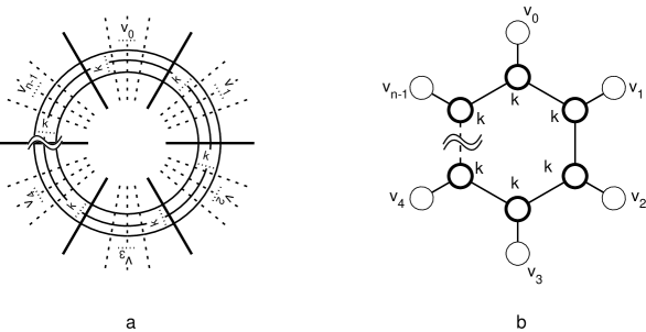
Figure 6: The D-brane configuration of the A-model and the corresponding quiver diagram.

It consists of $n$ NS 5-branes, $n$ sets of Dirichlet 5-branes, each set containing $v_{i},i=0,\ldots,n-1$ different Dirichlet 5-branes, and $k$ Dirichlet 3-branes. Applying the same rules as in the previous section we see that the three dimensional Dirichlet 3-brane worldvolume theory is an $N=4$ supersymmetric theory with gauge group and matter content associated with the quiver diagram 6b. This will be called the A-model. The gauge group is $U(k)^{n}$, one $U(k)$ for each node of the extended Dynkin diagram. There are two kinds of matter. As before, for each pair of gauge groups whose nodes are connected by an edge there is matter transforming as $({\bf k},{\bf k}^{\ast})$ under $U(k)\times U(k)$. In addition, there are $v_{i}$ matter fields transforming in the fundamental representation of the $i$th $U(k)$ gauge group.

We denote the A-model as $(U(k)^{n};\{v_{i}\})$. The Higgs branch of the A-model is the moduli space of instantons on a vector bundle $V$ over an ALE space of type $A_{n-1}$. More precisely, it describes the moduli space ${\cal M}_{k}(V)$ of instantons of instanton number $k$ on $V=\oplus{\cal R}_{i}^{\otimes v_{i}}$, with gauge group $U(V)$, where ${\cal R}_{i}$ are particular line bundles over the ALE space associated to the different representations of ${\bf Z}_{n}$ [5].

Performing an $SL(2,Z)$ transformation on the D-brane configuration in figure 6a yields a configuration which corresponds to the quiver diagram of figure 7 in the case where all $v_{i}\geq 1$.

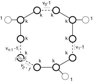
Figure 7: The quiver diagram of the B-model.

In the notations of [4], the B-model gauge theory in figure 7 is $(U(k)^{m};\{w_{i}\})$, where

$$\sum_{i=0}^{n-1}v_{i}=m,~{}~{}~{}~{}~{}~{}~{}\sum_{i=0}^{m-1}w_{i}=n\mskip 6.0mu.$$ (2.15)

The mirror map takes the following form: Denote by $\vec{m}_{i}^{(B)}$, $\sum_{l=0}^{j-1}w_{l}\leq i<\sum_{l=0}^{j}w_{l}$ the masses of the hypermultiplets in the B-model charged only under the $j^{\rm th}$ $U(k)$. In addition, there are $m$ masses of hypermultiplets charged under two $U(k)$’s. Using the freedom to shift the origin on the Coulomb branch, we can choose all these masses equal to the same value which we denote by $\vec{m}_{2f}^{(B)}$, and in addition we can choose $\vec{m}_{n-1}^{(B)}=0$. Then the relation between the FI parameters $\vec{\zeta}_{i}^{(A)}$ of the A-model and the masses of the B-model reads [4]

$$\sum_{l=0}^{i}\vec{\zeta}_{l}^{(A)} = \vec{m}_{i}^{(B)}+(\sum_{l=0}^{i}v_{l})\vec{m}_{2f}^{(B)}$$

$${}\sum_{l=0}^{n-1}\vec{\zeta}_{l}^{(A)} = (\sum_{l=0}^{n-1}v_{l})\vec{m}_{2f}^{(B)}.$$ (2.16)

In our case $\vec{m}_{2f}^{(B)}$ vanishes since the open string stretching between Dirichlet 3-branes which gives rise to a hypermultiplet charged under two $U(k)$’s is of zero length at the origin of the Coulomb branch. This is the analog of the adjoint hypermultiplet of the previous sections. Similarly, the sum of the FI parameters in the A-model is zero, which can be easily seen from (2.1).

As before, the $SL(2,Z)$ transformation replaces the NS and Dirichlet 5-branes, and exchanges $\vec{\omega}_{i}$ and $\vec{m}_{i}$. Using (2.1), the FI parameters of the A-model are related to the mass parameters of the B-model by

$$\vec{m}_{i}^{(B)}-\vec{m}_{i-1}^{(B)}=\vec{\zeta}_{i}^{(A)},~{}~{}~{}~{}~{}~{}~{}~{}~{}~{}i=1,...,n-1.$$ (2.17)

Equation (2.17) is equivalent to the mirror map (2.16) with $\vec{m}_{2f}^{(B)}=0$.

3 Duality for $\prod_{i}U(k_{i})$ Gauge Groups

In this section we generalize the examples of the previous section to dual models based on $\prod_{i}U(k_{i})$ gauge groups. Consider the quiver diagram in figure 8a, which encodes the field content of a $\prod_{i}U(k_{i})$ gauge theory.

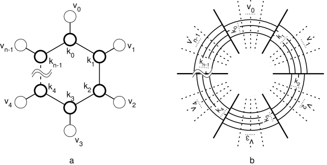
Figure 8: The D-branes configuration of the A-model and the corresponding quiver diagram.

We will analyze the mixed branches of this theory and find the criterion for complete Higgsing, both from a field theory viewpoint and via a consideration of D-brane configurations. This will enable us to find the procedure to construct the mirror partner of the model.

Denote the internal and external indices of the quiver diagram by the vectors ${\bf k}=(k_{0},\ldots,k_{n-1})$ and ${\bf v}=(v_{0},\ldots,v_{n-1})$ respectively. For a given choice of FI parameter $\zeta=(\vec{\zeta}_{0},\ldots,\vec{\zeta}_{n-1})$ the hypermultiplet moduli space of the gauge theory is the quiver variety ${\cal M}_{\zeta}({\bf k},{\bf v})$ which is a certain moduli space of instantons. When $\zeta$ is chosen to be generic, the gauge group is completely broken and ${\cal M}_{\zeta}({\bf k},{\bf v})$ is smooth. In this case, the theory only has a Higgs phase.

3.1 Mixed Branches in the Model with $\zeta=0$, $m=0$

When the FI parameters $\zeta$ and the bare masses $m$ are not generic, the moduli space of vacua consists of several branches touching each other at phase transition points (or lines, surfaces etc). We consider here the most special case $\zeta=0$, $m=0$. A mixed branch is characterized by a (conjugacy class of the) unbroken gauge group $G$. The classification of the possible unbroken gauge groups $G\subset\prod_{i}U(k_{i})$ is given in section 6 of [6] and section 3 and 4 of [12]. According to these, $G$ always takes the following form:

$$G=\prod_{a=1}^{p}U(\kappa_{a})\times\prod_{i=0}^{n-1}U(\ell_{i})\mskip 6.0mu.$$ (3.1)

Here $U(\kappa_{a})$ is the diagonal subgroup of $\prod_{i=0}^{n-1}U(\kappa_{a})_{i}\subset\prod_{i=0}^{n-1}U(k_{i})_{i}$, and $U(\ell_{i})$ is a subgroup of $U(k_{i})_{i}$. Let us denote $\tilde{k}_{i}=k_{i}-\sum_{a}\kappa_{a}-\ell_{i}$. Then, the mixed branch with unbroken gauge group (3.1) is the product ${\cal H}_{({\bf\tilde{k}},\kappa)}\times{\cal V}_{({\bf\tilde{k}},\kappa)}$, where ${\cal V}_{({\bf\tilde{k}},\kappa)}$ is a space of (quaternionic) dimension $\sum_{a}\kappa_{a}+\sum_{i}\ell_{i}$ and ${\cal H}_{({\bf\tilde{k}},\kappa)}$ is given by

$${\cal M}_{0}^{\rm reg}({\bf\tilde{k}},{\bf v})\times Sym^{\kappa}({\bf C}^{2}/{\bf Z}_{n}-\{0\})\mskip 6.0mu,$$ (3.2)

where ${\cal M}_{0}^{\rm reg}({\bf\tilde{k}},{\bf v})$ is the completely Higgsed phase of the model with internal indices ${\bf\tilde{k}}=(\tilde{k}_{0},\ldots,\tilde{k}_{r})$ and external indices ${\bf v}$. $Sym^{\kappa}X$ is the subspace of the symmetric product $Sym^{|\kappa|}X$, $|\kappa|=\sum_{a}\kappa_{a}$, consisting of configurations of ${|\kappa|}$-points in $X$ where $\kappa_{a}$ of them are in the same position.

We can find a corresponding branch in a three and 5-brane configuration. We assume that the nonemptyness of ${\cal M}_{0}^{\rm reg}({\bf k},{\bf v})$ corresponds to the existence of a complete Higgs phase in the brane picture. It will be shown in the next subsection that this is indeed correct. The branch consists of configurations of Dirichlet 3-branes where $\ell_{i}$ of the $k_{i}$ Dirichlet 3-branes in the $i^{\rm th}$ interval between the NS 5-branes are constrained to end on the NS 5-branes, and there are $|\kappa|$ Dirichlet 3-branes without boundary moving freely from the NS 5-branes but $\kappa_{a}$ of them ($a=1,\ldots,p$) are constrained to have the same position in the ($x^{7},x^{8},x^{9}$) direction. In addition, there are other Dirichlet 3-branes, that are partly generated by passing Dirichlet 5-branes through NS 5-branes, as will be explained in detail in the following.

3.2 Criterion for Existence of Complete Higgs Phase

In [4] we proposed a condition for the existence of a complete Higgs phase in the models corresponding to quiver diagrams with indices $({\bf k},{\bf v})$. It is given by (see e.g. equation (8.5))

$$v_{i}\geq 2k_{i}-k_{i-1}-k_{i+1}.$$ (3.3)

In fact the same issue is discussed in [6] and solved in [12]. The criterion (Corollary 10.9 of [12]) is indeed (3.3) provided that the condition

$$\sum_{i=0}^{n-1}v_{i}\geq 2$$ (3.4)

holds. We now derive (3.3) and (3.4) from the three and 5-brane picture. In order to get a complete Higgs phase we have to take all the 3-branes off the NS 5-branes and constrain them to end on the Dirichlet 5-branes. We do this as in [8] by moving Dirichlet 5-branes through NS 5-branes creating new Dirichlet 3-branes between them. Let us focus on the neighborhood of the $i^{\rm th}$ interval of NS 5-branes in figure 9.

Figure 9: The $i^{\rm th}$ interval of NS 5-branes.

We distinguish the following three cases: (i) $k_{i}\geq k_{i-1},k_{i+1}$, (ii) $k_{i+1}\geq k_{i}\geq k_{i-1}$ and (iii) $k_{i}\leq k_{i+1},k_{i-1}$. We will derive the condition for taking the Dirichlet 3-branes off the NS 5-branes in the order (i)$\Rightarrow$(ii)$\Rightarrow$(iii) inductively. In case (i) we move $k_{i}-k_{i-1}$ Dirichlet 5-branes in the interval to the left-next interval and $k_{i}-k_{i+1}$ to the right-next interval. This is possible if and only if $v_{i}\geq(k_{i}-k_{i-1})+(k_{i}-k_{i+1})$ which is the condition (3.3). In case (ii), given that the Dirichlet 5-branes have been moved as in step (i), $k_{i+1}-k_{i}$ Dirichlet 5-branes enter in the interval from the right-next one. So now, there are $v_{i}+k_{i+1}-k_{i}$ Dirichlet 5-branes. Then, we only have to move $k_{i}-k_{i-1}$ of them to the left-next interval, which is possible if and only if $v_{i}+k_{i+1}-k_{i}\geq k_{i}-k_{i-1}$. Finally in the case (iii) where the condition (3.3) is trivially satisfied, given (i) and (ii), $k_{i+1}-k_{i}$ Dirichlet 5-branes enter from the right while $k_{i-1}-k_{i}$ from the left. At this stage it is obvious that all the Dirichlet 3-branes can be taken off the NS 5-branes. Now we have to find a phase where all the Dirichlet 3-branes are constrained to end on Dirichlet 5-branes. If there is no Dirichlet 5-brane, it is impossible. If there is only one Dirichlet 5-brane as in figure 10, even though all the 3-branes can intersect with it, we can easily take them off because none of them has a boundary, and there is no complete Higgs phase. If there are two or more Dirichlet 5-branes as in figure 11, then, there is obviously a phase where all the 3-branes end on Dirichlet 5-branes at their boundaries which cannot be taken off the Dirichlet 5-branes. Thus, we rederived the condition (3.4).

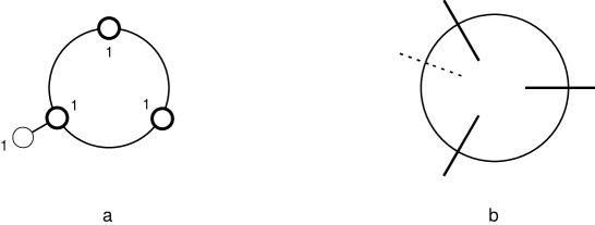
Figure 10: A configuration with one Dirichlet 5-brane where there is no complete Higgsing since the condition (3.4) is not satisfied.

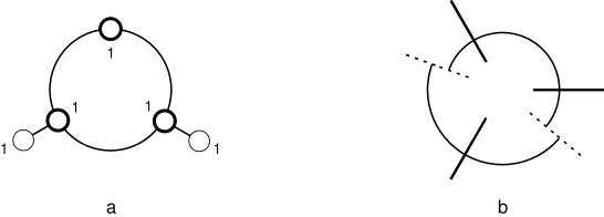
Figure 11: A modification of figure 10, with two Dirichlet 5-branes where there is a complete Higgsing since both conditions (3.3) and (3.4) are satisfied.

As an application of the condition for complete Higgsing, we will show that when two Dirichlet 5-branes pass each other the field theory may undergo a phase transition in the D-brane moduli space. To be precise, 5-branes of the same type do not have to pass each other but can be exchanged by moving them in the three coordinates transverse to their worldvolume.

Consider the quiver diagram of figure 12a. The intersecting brane configuration corresponding to it can be brought by the usual rule for Dirichlet 5-branes passing an NS 5-brane to the form of figure 12c. If we allow a Dirichlet 5-brane to pass another Dirichlet 5-brane we get the brane configuration of figure 13a.

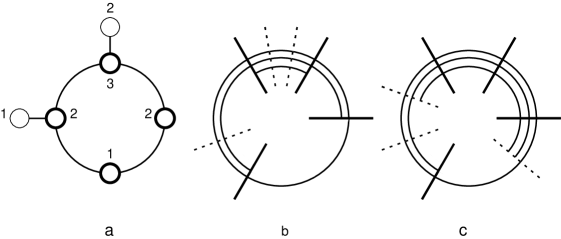
Figure 12: A quiver, its Coulomb branch description via D-branes in 12b, and its Higgs branch description in 12c.

Figure 13: The D-brane configuration 13a is derived from figure 12c if we we allow a Dirichlet 5-brane to pass another Dirichlet 5-brane. 13b is the $SL(2,Z)$ dual of 13a. The quiver in 13c corresponding to 13b is a false mirror of 12a.

Using $SL(2,Z)$ transformations on figure 13a we will conclude that the quiver diagram of figure 13c is the mirror of the quiver diagram of figure 12a. However, this is incorrect since the model of figure 12a has a Coulomb phase while the model of figure 13c does not have a complete Higgs phase, since the condition (3.3) is not satisfied. One can also check this by counting the dimensions of the vector multiplet and hypermultiplet moduli spaces of the models. Therefore we are led to a contradiction. This implies that when two 5-branes of the same type pass each other, the field theory content on the D3 brane is changed — we have a nontrivial phase transition on its worldvolume. This phenomenon has a simple interpretation in terms of D-branes. The coupling contants, as well as the Fayet-Iliopoulos and mass parameters of the D3 brane worldvolume theory are determined by the positions of the various 5-branes. Varying them is simply moving around in the 5-brane moduli spaces. Incidentally, these moduli spaces also have a gauge theoretic interpretation, i.e. moduli spaces of the supersymmetric gauge theories on the 5-brane worldvolumes. D-branes thus link different field theories as phases corresponding to different regions of the brane moduli space.

This is one of the most important concepts emerging from this construction. It has much in common with the conifold transition [21]. Here we encountered phase transitions in field theory while moving smoothly in the D-brane moduli space. The conifold transition is a phase transition from the supergravity field theory viewpoint and is smooth in the closed string theory.

3.3 Mirror Pairs

The above consideration of three and 5-brane configurations leads to a recipe for the construction of mirror pairs. The mirror of the model based on affine $A_{n-1}$ Dynkin diagram with indices $({\bf k},{\bf v})$ is the model based on affine $A_{m-1}$ Dynkin diagram with indices $({\bf l},{\bf w})$, ${\bf l}=(l_{0},\ldots,l_{m-1})$, ${\bf w}=(w_{0},\ldots,w_{m-1})$, which are given in the following way. Without loss of generality, we may assume that $k_{0}=\max\{k_{i}\}$. Let us introduce the notations ${\bf\tilde{v}}={\bf v}-{\bf C}_{n}{\bf k}$ and ${\bf\tilde{w}}={\bf w}-{\bf C}_{m}{\bf l}$ where ${\bf C}_{n}$ and ${\bf C}_{m}$ are the Cartan matrices for the affine Lie algebras $\widehat{sl(n)}$ and $\widehat{sl(m)}$ respectively. Then, ${\bf w}$ and ${\bf\tilde{w}}$ are given by

$${\bf w} = (1,\underbrace{0,\ldots,0}_{\tilde{v}_{1}-1},1,\underbrace{0,\ldots,0}_{\tilde{v}_{2}-1},1,\ldots,1,\underbrace{0,\ldots,0}_{\tilde{v}_{n-1}},1,\underbrace{0,\ldots,0}_{\tilde{v}_{0}-1})$$ (3.5)

$${\bf\tilde{w}} = (\underbrace{0,\ldots,0}_{k_{0}-k_{1}},1,\underbrace{0,\ldots,0}_{v_{1}-1},1,\underbrace{0,\ldots,0}_{v_{2}-1},1,\ldots,1,\underbrace{0,\ldots,0}_{v_{n-1}},1,\underbrace{0,\ldots,0}_{v_{0}+k_{1}-k_{0}-1}).$$ (3.6)

Here, if there is a space of negative length $v_{i}-1=-1$, the left-next entry is added to the right next entry. If the negative space appears in the right extreme, the left-next entry is added to the first entry. Given ${\bf w}$ and ${\bf\tilde{w}}$, the vector ${\bf l}$ is determined up to an ambiguity of adding $(1,1,\ldots,1)$. This is fixed by saying that $l_{0}=k_{0}$. Note that $n$ and $m$ are related by

$$m=\sum_{i=0}^{n-1}v_{i},\qquad n=\sum_{\imath=0}^{m-1}w_{\imath}$$ (3.7)

We can associate to vectors of indices Young diagrams ${\bf v},{\bf\tilde{v}},{\bf w},{\bf\tilde{w}}$ $\rightarrow$ $Y({\bf v}),Y({\bf\tilde{v}}),Y({\bf w}),Y({\bf\tilde{w}})$. Here, $Y({\bf v}),Y({\bf\tilde{v}})$ are Young diagrams whose rows have lengths $\sum_{i=0}^{j}v_{i},j=0,\ldots,n-1$ and $\sum_{i=0}^{j}\tilde{v}_{i},j=0,\ldots,n-1$. The Young diagrams $Y({\bf w}),Y({\bf\tilde{w}})$ have columns of lengths $\sum_{i=q-j}^{q}w_{i},j=0,\ldots,m-1$ and $\sum_{i=\tilde{q}-j}^{\tilde{q}}\tilde{w}_{i},j=0,\ldots,m-1$, where $q$ and $\tilde{q}$ are the largest indices such that $w_{q}\neq 0$, $\tilde{w}_{\tilde{q}}\neq 0$. The Young diagrams are related by

$$Y({\bf v})={}^{t}Y({\bf\tilde{w}}),\qquad Y({\bf w})={}^{t}Y({\bf\tilde{v}}),$$ (3.8)

where ${}^{t}Y$ is the transposition of $Y$ along the NorthWest-SouthEast diagonal. This generalizes the transposition rule [4] of the models with common internal indices in which ${\bf\tilde{v}}={\bf v}$, ${\bf\tilde{w}}={\bf w}$.

As an illustration, consider gauge theory associated to the quiver diagram given in figure 14a. One can find its mirror by considering the corresponding brane configuration, moving D5 branes in an appropriate way, and performing an $SL(2,{\bf Z})$ transformation. The result is given in figure 14b, the corresponding Young diagrams in figure 15 and 16.

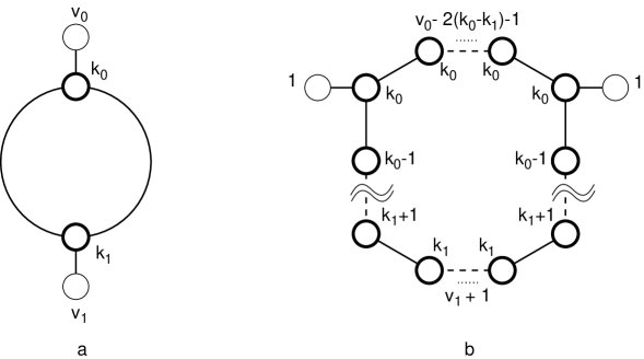
Figure 14: An example of a mirror pair.

Figure 15: Young diagram for the model in figure 14a: Figure 15a is $Y({\bf v})$ and figure 15b is $Y({\bf\tilde{v}})$ .

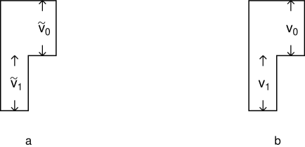
Figure 16: Young diagram for the model in figure 14b: Figure 16a is $Y({\bf w})$ and figure 16b is $Y({\bf\tilde{w}})$ .

3.4 Mirror Symmetry and Level-Rank Duality

In [6, 12] Nakajima showed that there is an action of the affine Lie algebra $\widehat{sl(n)}$ on the middle dimensional homology groups ${\rm H}_{mid}({\cal M}_{\zeta}({\bf k},{\bf v}))$ of the moduli spaces ${\cal M}_{\zeta}({\bf k},{\bf v})$ of the models based on the affine $A_{n-1}$ Dynkin diagram where $\zeta$ is chosen to be generic. More precisely, for a fixed ${\bf v}$, there is an action of the affine Lie algebra $\widehat{sl(n)}$ on the vector space

$$\bigoplus_{{\bf k}}{\rm H}_{mid}({\cal M}_{\zeta}({\bf k},{\bf v}))$$

where ${\bf k}$ runs over all possible internal indices. It is the irreducible integrable highest weight representation of highest weight $\Lambda_{{\bf v}}$ where ${\rm H}_{mid}({\cal M}_{\zeta}({\bf k},{\bf v}))$ is the weight space for the weight $\Lambda_{{\bf v}}-\alpha_{{\bf k}}$ (Theorem 10.16 of [6], Theorem 10.3 of [12]). The symbols $\Lambda_{{\bf v}}$ and $\alpha_{{\bf k}}$ in the statement are defined by $\Lambda_{{\bf v}}=\sum_{i=0}^{r}v_{i}\Lambda_{i},$ $\alpha_{{\bf k}}=\sum_{i=0}^{r}k_{i}\alpha_{i},$, where $\Lambda_{i}$ are the fundamental affine weights and $\alpha_{i}$ are the simple affine roots. It is interesting to note that the middle dimensional homology of the Higgs branch of the model based on the affine $A_{n-1}$ Dynkin diagram with indices $({\bf k},{\bf v})$ is a weight space of a representation of $\widehat{sl(n)}$ at level $m$ while the one of the mirror (based on the affine $A_{m-1}$ Dynkin diagram with indices $({\bf l},{\bf w})$) is a weight space of a representation of $\widehat{sl(m)}$ at level $n$. Indeed the condition (3.3) for existence of complete Higgs phase in the model with $\zeta=m=0$ simply says that $\Lambda_{{\bf v}}-\alpha_{{\bf k}}$ is non-negative, which implies that $\Lambda_{{\bf v}}-\alpha_{{\bf k}}$ is a weight of the integrable representation of highest weight $\Lambda_{{\bf v}}$ (see [22] Proposition 12.5). The other condition (3.4) shows that the mirror is also based on an affine Dynkin diagram. This strongly reminds us of the so called level-rank duality in two dimensional conformal field theories, solvable statistical models, and quantum groups (see [23] and references therein). Usually, level-rank duality is stated in terms of transposition of Young diagrams which can be contrasted with (3.8). It would be interesting to pursue the relation between mirror symmetry and level-rank duality further and find its physical interpretation. In particular, we would like to know the meaning of the curious fact that the mirror symmetry does not map highest weights to highest weights, and whether the middle-dimensional homologies of the moduli spaces have any interpretation in field theory.

4 Abelian Dual Pairs

In this section we describe a large class of dual pairs of Abelian $N=4$ gauge theories with matter. In fact, modulo some subtleties, we will be able to find the dual of any given Abelian gauge theory with matter, as long as there is some matter charged under each $U(1)$ gauge group. If this would not be the case, part of the theory would be a pure $N=4$ $U(1)$ Yang-Mills theory. The moduli space of this theory contains only a Coulomb branch with metric (for notations see [4])

$$ds^{2}=\frac{1}{e^{2}}d\vec{r}^{2}+e^{2}d\phi^{2}$$ (4.1)

which describes a cylinder ${\bf R}^{3}\times S^{1}_{e}$, where $S^{1}_{e}$ is a circle with radius $e$, $e$ being the gauge coupling. One could argue that in the “infrared” limit $e^{2}\rightarrow\infty$ this metric becomes the flat metric on ${\bf R}^{4}$, as the circle get decompactified. The dual theory of pure $U(1)$ Yang-Mills theory is then easily found, it is a theory with one free hypermultiplet and no gauge group, whose moduli space contains just a Higgs branch ${\bf R}^{4}$. We will in what follows never consider this trivial mirror pair

$$\mbox{pure $U(1)$ gauge theory}\leftrightarrow\mbox{neutral hypermultiplet},$$ (4.2)

but one can always add arbitrary many copies of it to the Abelian dual pairs that we describe below.

Let us now take any Abelian gauge theory with gauge group $U(1)^{N_{c}}$ and with $N_{f}$ flavors, and assume that it does not contain pure gauge groups or neutral hypermultiplets. We further assume that after a change of basis the hypermultiplets can be arranged in two sets $Q_{i}$, $i=1\ldots N_{c}$ and $Q_{\alpha}$, $\alpha=1\ldots N_{f}-N_{c}$, such that $Q_{i}$ has charge $1$ under the $i$th $U(1)$ and is neutral with respect to the others. The charge of $Q_{\alpha}$ under the $i$th $U(1)$ gauge group can be an arbitrary integer which we denote by $m_{i\alpha}$. This situation cannot always be achieved, take for example one $U(1)$ with two hypermultiplets with charges $2$ and $3$. We will discuss the general situation later.

The total charge matrix for the hypermultiplets $Q_{i}$ and $Q_{\alpha}$ is the $N_{c}\times N_{f}$ matrix $({\bf 1}|m)$. We now claim that the dual of this theory is the $N=4$ gauge theory with gauge group $U(1)^{N_{f}-N_{c}}$ and $(N_{f}-N_{c})\times N_{f}$ charge matrix $({\bf 1}|-m^{t})$,

$$U(1)^{N_{c}},\mbox{\rm charges }({\bf 1}|m)\leftrightarrow U(1)^{N_{f}-N_{c}},\mbox{\rm charges }({\bf 1}|-m^{t}).$$ (4.3)

This is slightly reminiscent of the non-Abelian duality in $N=1$ theories in four dimensions [24], where the dual theories have gauge groups $SU(N_{c})$ and $SU(N_{f}-N_{c})$.

As a first check, we compute the dimensions for the Coulomb and Higgs branches. The first model has a Coulomb branch of (quaternionic) dimension $N_{c}$, and a Higgs branch of dimension $N_{f}-N_{c}$, while the second model has these numbers interchanged, as it should. Furthermore, the first model has $N_{c}$ Fayet-Iliopoulos parameters $\vec{\zeta}^{A}_{i}$, and $N_{f}$ mass parameters. We can use the freedom to choose the origin in the Coulomb branch to choose the mass parameters of $Q_{i}$ to be zero, so that all what remains is the $N_{f}-N_{c}$ mass parameters $\vec{m}^{A}_{\alpha}$ of the $Q_{\alpha}$. The dual theory has $N_{f}-N_{c}$ Fayet-Iliopoulos parameters $\vec{\zeta}^{B}_{\alpha}$ and $N_{c}$ independent mass parameters $\vec{m}^{B}_{i}$. The number of Fayet-Iliopoulos and mass parameters is indeed interchanged under the duality. In fact, we will demonstrate later that the precise mirror map is simply

$$\vec{\zeta}^{A}_{i}\leftrightarrow\vec{m}^{B}_{i},\qquad\vec{m}^{B}_{\alpha}\leftrightarrow\vec{\zeta}^{A}_{\alpha}.$$ (4.4)

Before giving a string theory and a field theory proof of this duality, we will first give an example. Consider a $U(1)$ theory with $n$ fundamentals, all with charge one. The dual theory has $U(1)^{n-1}$ gauge symmetry and charge matrix

$$\left(\begin{array}[]{ccc}1\!\!&&\\[-2.84544pt] &\!\ddots\!&\\[-2.84544pt] &&\!\!1\end{array}\left|\begin{array}[]{c}-1\\[-2.84544pt] \vdots\\[-2.84544pt] -1\end{array}\right.\right)$$ (4.5)

and after a change of basis one sees that this is precisely the dual gauge theory proposed in [2].

4.1 String Theory Proof

In [2],[25] it was proposed that mirror symmetry in three-dimensional gauge theories should be a consequence of T-duality of type IIA and IIB string theory. In [4] we elaborated on this proposal to provide evidence for the dualities proposed in that paper. In addition to this, various D-brane techniques to study three-dimensional gauge symmetries and their mirror symmetry have been developed [15, 4, 7, 8]. In the latter case, matter usually appears through open strings connecting D-branes, and is therefore charged under at most two gauge groups. Since we are interested in the case where matter can be charged under arbitrary many gauge groups, the string theory analysis using T-duality will be more useful.

We therefore view the three-dimensional gauge theories as being obtained from a compactification of the type IIA string on $CY\times S^{1}_{R}$. To get a field theory in three dimensions, we have to take a limit where $R\rightarrow 0$ and $\alpha^{\prime}\rightarrow 0$, while keeping $R/\sqrt{\alpha^{\prime}}$ finite. The type IIA compactification is T-dual to IIB on $CY\times S^{1}_{\alpha^{\prime}/R}$, and the radius of this circle also shrinks to zero. Under T-duality, the vector and hypermultiplet moduli spaces are interchanged, which corresponds exactly to what happens in mirror symmetry in three dimensions.

In order to apply T-duality, we first have to construct a singular Calabi-Yau manifold so that type IIA compactified on it will give rise to a $U(1)^{N_{c}}$ gauge theory in three dimensions, with matter with charge matrix $({\bf 1}|m)$. Only the local structure of the singularity is relevant for the field theory [26]. In order to get $N_{f}$ hypermultiplets coming from wrapping D2-branes on two-cycles, we need $N_{f}$ vanishing two-cycles, which we will denote by $C_{i}$ and $C_{\alpha}$. Furthermore, in order to get a $U(1)^{N_{c}}$ gauge symmetry, we need that these $N_{f}$ two-cycles satisfy $N_{f}-N_{c}$ relations in homology, so that there are only $N_{c}$ homologically independent two-cycles. Since the charges of the hypermultiplets can be read off from the homology relations, we find that in our case the homology relations have to be $[C_{\alpha}]=\sum_{i}m_{i\alpha}[C_{i}]$. For finite sizes of the two-cycles we are in the Coulomb branch of the gauge theory. After applying T-duality we end up in the Higgs branch of the dual theory. It is very difficult to recognize the gauge field and matter content of a gauge theory in the Higgs phase, and therefore it is better to first go to the Higgs phase of the original theory, and to apply T-duality after that, so as to end up in the Coulomb branch of the dual theory. The transition of the Coulomb branch to the Higgs branch is geometrically given by a conifold or extremal transition [21, 27, 28]. In type IIA string compactification, it is the process in which two-cycles shrink to points which are then deformed to three-cycles with finite volume. Denote by $\tilde{C}_{i}$ and $\tilde{C}_{\alpha}$ the three cycles obtained after shrinking the corresponding two-cycle and replacing it by a three-cycle. To find out the homology relations between these three-cycles, we use the results in [28]. Before shrinking the two-cycles, there are “magnetic” four cycles $C_{i}^{\ast}$ which are dual to $C_{i}$ in homology. In other words, the intersection numbers are $<C_{i}^{\ast}|C_{j}>=\delta_{ij}$ and $<C_{i}^{\ast}|C_{\alpha}>=m_{i\alpha}$. After the conifold transition, these magnetic four-cycles have become four-chain (denoted again by $C_{i}^{\ast}$), with boundary given by

$$\partial C_{i}^{\ast}=\sum_{j}<C_{i}^{\ast}|C_{j}>\tilde{C}_{j}+\sum_{\alpha}<C_{i}^{\ast}|C_{\alpha}>\tilde{C}_{\alpha}.$$ (4.6)

There are therefore $N_{c}$ relations between the $N_{f}$ three-cycles, given by

$$[\tilde{C}_{i}]=-\sum_{\alpha}m_{i\alpha}[\tilde{C}_{\alpha}].$$ (4.7)

The Calabi-Yau with these vanishing three-cycles describes the Higgs phase of the original theory if we put the type IIA string on it, and after T-duality it should describe the Coulomb branch of the dual theory if we put the type IIB string on it. In type IIB compactifications, vanishing three-cycles give rise to matter by wrapping D3-branes on them, the number of $U(1)$ gauge groups is the number of homologically independent three-cycles, and the charges can be read off from the homology relations. By inspection of (4.7), we see that the dual theory is a $U(1)^{N_{f}-N_{c}}$ gauge theory, with charge matrix $({\bf 1}|-m^{t})$. Notice that the homology relations (4.7) are such that the conifold transition is indeed possible [28]. This gives a string theory proof of the proposed duality. In order to also derive the mirror map and to find the explicit forms of the metrics on the Coulomb and Higgs branches of the moduli space, we now turn to a field theory proof of the duality.

4.2 Field Theory Proof

The field theory proof will simply consist of an explicit computation of the metrics on the Higgs and Coulomb branches of the moduli space of the $U(1)^{N_{c}}$ gauge theory. The Coulomb branch of the moduli space is given a hyperkähler manifold, whose metric can be computed in perturbation theory. Because the gauge group is Abelian, there can be no monopole corrections to the metric and perturbation theory should give the full answer. Each $U(1)$ vector multiplet contains three scalars, whose expectation values we denote by $\vec{r}_{i}$, $i=1,\ldots,N_{c}$. In addition, there are $N_{c}$ angular variables $\phi_{i}$ which is the expectation value of the scalar dual to the gauge fields, and which is periodic with period $2\pi$. Constant shifts of these angular variables $\phi_{i}$ is a symmetry of the theory that is unbroken in perturbation theory, and gives rise to $N_{c}$ triholomorphic $U(1)$ isometries of the Coulomb branch metric. Such metrics can always be written in the form [29, 30]

$$ds^{2}=g_{ij}d\vec{r}_{i}d\vec{r}_{j}+(g^{-1})_{ij}(d\phi_{i}+\vec{\omega}_{ik}\cdot d\vec{r}_{k})(d\phi_{j}+\vec{\omega}_{jl}\cdot d\vec{r}_{l})$$ (4.8)

where

$$\vec{\nabla}_{i}g_{jk} = \vec{\nabla}_{j}g_{ik}$$

$${}\frac{\partial}{\partial r^{p}_{i}}\omega^{q}_{jk}-\frac{\partial}{\partial r^{q}_{j}}\omega^{p}_{ik} = \epsilon_{pqr}\frac{\partial}{\partial r^{r}_{i}}g_{jk}.$$ (4.9)

Either by comparing to known cases, or by doing a direct one-loop calculation, one finds that through one loop the metric $g_{ij}$ is given by

$$g_{ij}=\frac{\delta_{ij}}{e^{2}}+\frac{\delta_{ij}}{|\vec{r}_{i}|}+\sum_{\alpha}\frac{m_{i\alpha}m_{j\alpha}}{|\vec{r}_{k}m_{k\alpha}+\vec{m}_{\alpha}|}$$ (4.10)

where $e$ is the bare gauge coupling. Mirror symmetry will only hold in the limit where $e\rightarrow\infty$. Although we have no rigorous proof, it seems plausible that $g_{ij}$ does not receive any further higher loop corrections. If there would be a good off-shell formulation of $N=4$ multiplets in three-dimensions, the first term of the metric (4.8) would come from an F-term, and one could use this to argue in favor of the absence of higher loop corrections to $g_{ij}$. The absence of higher loop corrections is also supported by the string theory considerations in the previous section, and we will assume this to be the case from now on.

It remains to compute the metric on the Higgs branch, which is given by an hyperkähler quotient of an $N_{f}-N_{c}$ quaternionic dimensional vector space with the flat metric by the action of the group $U(1)^{N_{c}}$. Luckily, the metric on the Higgs branch is not subject to perturbative or non-perturbative corrections, and the classical considerations will be exact. The moment map equations for the hyperkähler quotient are certain quadratic equations for the expectation values of the scalar fields in the hypermultiplets. However, since we are dealing with an Abelian hyperkähler quotient, we can perform a change of variables that linearizes the moment map equations, see [31] and section 4.3 of [4]. In this change of variables, we replace the two complex numbers that are the expectation values of the two complex scalars in a hypermultiplet by a three vector and an angular variable. Denote the vector and angular variable coming from $<Q_{i}>$ by $\vec{s}_{i},\psi_{i}$, and those coming from $<Q_{\alpha}>$ by $\vec{s}_{\alpha},\psi_{\alpha}$. Then the flat metric for $<Q_{i}>$ and $<Q_{\alpha}>$ in terms of the new variables reads

$$ds^{2} = \sum_{i}\left(\frac{1}{|\vec{s}_{i}|}d\vec{s}_{i}d\vec{s}_{i}+|\vec{s}_{i}|(d\psi_{i}+\vec{\omega}_{i}\cdot d\vec{s}_{i})^{2}\right)$$ (4.11)

$$+\sum_{\alpha}\left(\frac{1}{|\vec{s}_{\alpha}|}d\vec{s}_{\alpha}d\vec{s}_{\alpha}+|\vec{s}_{\alpha}|(d\psi_{\alpha}+\vec{\omega}_{\alpha}\cdot d\vec{s}_{\alpha})^{2}\right),$$

where $\vec{\omega}$ is determined by means of (4.9). The $\vec{s}$ are clearly the natural variables to compare the Higgs branch metric to the Coulomb branch metric. The moment map equations in terms of the new variables read

$$\vec{\mu}_{i}\equiv\vec{s}_{i}+\sum_{\alpha}m_{i\alpha}\vec{s}_{\alpha}=\vec{\zeta}_{i},\qquad i=1,\dots,N_{c}$$ (4.12)

where the $\vec{\zeta}$ are the Fayet-Iliopoulos parameters. The vector fields that generate the action of $U(1)^{N_{c}}$ are

$$V_{i}=\frac{\partial}{\partial\psi_{i}}+\sum_{\alpha}m_{i\alpha}\frac{\partial}{\partial\psi_{\alpha}}.$$ (4.13)

The moment map equations can be used to solve for $\vec{s}_{i}$ in terms of $\vec{s}_{\alpha}$. If we substitute this solution in (4.11), we find the metric on the constrained manifold $\vec{\mu}^{-1}(\vec{\zeta})$. Subsequently, we can use the $U(1)^{N_{c}}$ symmetry to gauge fix $\psi_{i}=0$, so that $\vec{s}_{\alpha},\psi_{\alpha}$ are the coordinates on the hyperkähler quotient ${\cal M}=\vec{\mu}^{-1}(\vec{\zeta})/U(1)^{N_{c}}$. To compute the metric on the hyperkähler quotient, we need to project its tangent vectors in the direction perpendicular to the gauge group. For example, let us compute the inner product of the vectors $V_{\alpha}=\partial/\partial\psi_{\alpha}$ and $V_{\beta}=\partial/\partial\psi_{\beta}$ on ${\cal M}$. If $(,)$ denotes the inner product on $\vec{\mu}^{-1}(\vec{\zeta})$, and $(,)_{\cal M}$ that on ${\cal M}$, then

$$(V_{\alpha},V_{\beta})_{\cal M}=(V_{\alpha},V_{\beta})-(V_{\alpha},V_{i})(N^{-1})^{ij}(V_{j},V_{\beta})$$ (4.14)

where $N_{ij}=(V_{i},V_{j})$. Explicitly, this becomes

$$(V_{\alpha},V_{\beta})_{\cal M} = |\vec{s}_{\alpha}|\delta_{\alpha\beta}-|\vec{s}_{\alpha}|m_{i\alpha}(N^{-1})^{ij}|\vec{s}_{\beta}|m_{j\beta}$$

$$N_{ij} = |\vec{s}_{i}|\delta_{ij}+m_{i\alpha}|\vec{s}_{\alpha}|m_{j\alpha}$$ (4.15)

where $\vec{s}_{i}$ is expressed in terms of $\vec{s}_{\alpha}$ by means of (4.12). After some algebra, one can show that $(V_{\alpha},V_{\beta})_{\cal M}$ is the inverse of the matrix $g_{\alpha\beta}=|\vec{s}_{\alpha}|^{-1}\delta_{\alpha\beta}+m_{i\alpha}|\vec{s}_{i}|^{-1}m_{j\beta}.$ In a similar fashion one can find all the remaining components of the metric on ${\cal M}$, with as final result that the metric on the Higgs branch is given by

$$ds^{2}=g_{\alpha\beta}d\vec{s}_{\alpha}d\vec{s}_{\beta}+(g^{-1})_{\alpha\beta}(d\psi_{\alpha}+\vec{\omega}_{\alpha\gamma}\cdot d\vec{s}_{\gamma})(d\psi_{\beta}+\vec{\omega}_{\beta\delta}\cdot d\vec{s}_{\delta})$$ (4.16)

with

$$g_{\alpha\beta}=\frac{\delta_{\alpha\beta}}{|\vec{s}_{\alpha}|}+\sum_{i}\frac{m_{i\alpha}m_{i\beta}}{|\vec{\zeta}_{i}-m_{i\gamma}\vec{s}_{\gamma}|}.$$ (4.17)

By comparing (4.10) and (4.17), we immediately see that the duality $m\leftrightarrow-m^{t}$ indeed exchanges the metrics on the Higgs and Coulomb branches, and that the mirror map is given by (4.4).

4.3 General Charges

The duality we considered so far was restricted to the case where the charge matrix had the specific form $({\bf 1}|m)$. Here we consider what happens if the charge matrix has a generic form $(a_{ij}|b_{i\alpha})$, with $a_{ij}$ a non-degenerate matrix. This situation can always be achieved, if necessary after a relabeling of the hypermultiplets. In addition, we have the freedom to choose a different basis for the generators of the $U(1)^{N_{c}}$ gauge group. In order to keep the same gauge group, and not a multiple cover of it, different bases must be related by an $N_{c}\times N_{c}$ integer-valued matrix $c_{ij}$ with determinant $\pm 1$. Thus, the theory with charge matrix $(a_{ij}|b_{i\alpha})$ is equivalent to the theory with charge matrix $(c_{ik}a_{kj}|c_{ik}b_{k\alpha})$. If the determinant of $a_{ij}$ is $\pm 1$, we can choose $c=a^{-1}$, and we are back in the situation we already discussed. It remains therefore to discuss the case where the determinant of $a$ is not equal to $\pm 1$.

First, we consider what happens to a general metric of the form (4.8) if we introduce new variables $\phi_{i}=c_{ij}\phi^{\prime}_{j}$, with $c_{ij}$ some non-degenerate integer-valued matrix. If we at the same time replace $\vec{r}_{i}=\vec{r}^{\prime}_{j}(c^{-1})_{ji}$, $g_{ij}=c_{ik}c_{jl}g^{\prime}_{kl}$ and $\vec{\omega}_{ij}=c_{ik}c_{jl}\vec{\omega}^{\prime}_{kl}$, the metric keeps the form (4.8) in terms of the primed variables, and (4.9) remains satisfied. If we assume that the $\phi^{\prime}_{i}$ are also periodic with period $2\pi$, then the metric in the primed variables describes a $\Gamma$-fold cover of the metric in the unprimed variables, where $\Gamma$ is the finite group ${\bf Z}^{n}/c({\bf Z}^{n})$.

The above remarks are useful when we study the Higgs branch of the theory with charges $(a_{ij}|b_{i\alpha})$. The moment map equations read

$$a_{ij}\vec{s}_{i}+b_{i\alpha}\vec{s}_{\alpha}=\vec{\zeta}_{i}$$ (4.18)

and these can again be used to solve for $\vec{s}_{i}$ in terms of $\vec{s}_{\alpha}$. In addition, the $U(1)^{N_{c}}$ symmetry can be used to gauge $\psi_{i}=0$, but in contrast to the previous case, this does not yet completely fix the $U(1)^{N_{c}}$ gauge symmetry. A finite subgroup $\Gamma$ still acts on the $\psi_{\alpha}$, while preserving $\psi_{i}=0$. This means that (4.16), with $\vec{\zeta}_{i}$ replaced by $(a^{-1})_{ik}\vec{\zeta}_{k}$ and $m_{i\alpha}$ by $(a^{-1})_{ik}b_{k\alpha}$, describes in fact a $\Gamma$-fold cover of the Higgs branch. The finite group $\Gamma$ is given by

$$\Gamma=\frac{{\bf Z}^{N_{f}}\oplus b^{t}(a^{-1})^{t}({\bf Z}^{N_{c}})}{{\bf Z}^{N_{f}}}.$$ (4.19)

In order to find the metric on the Higgs branch itself, we have to mod out by the action of the group $\Gamma$, which is similar to the situation described above where we replaced $\phi_{i}=c_{ij}\phi^{\prime}_{j}$ etc. Here, we need to replace $\psi_{\alpha}=c_{\alpha\beta}\psi^{\prime}_{\beta}$, with similar replacements for the other variables. In order to correctly implement the action of the group $\Gamma$, the $N_{f}\times N_{f}$ matrix $c_{\alpha\beta}$ must be chosen in such a way that its columns form a basis for the lattice ${\bf Z}^{N_{f}}\oplus b^{t}(a^{-1})^{t}({\bf Z}^{N_{c}})$. This then finally yields the following metric on the Higgs branch, where we dropped the primes

$$g_{\alpha\beta}=\sum_{\gamma}\frac{(c^{-1})_{\alpha\gamma}(c^{-1})_{\beta\gamma}}{|\vec{s}_{\delta}c^{-1}_{\delta\gamma}|}+\sum_{i}\frac{(a^{-1}b(c^{-1})^{t})_{i\alpha}(a^{-1}b(c^{-1})^{t})_{i\beta}}{|(a^{-1})_{ij}\vec{\zeta}_{j}-(a^{-1}b(c^{-1})^{t})_{i\gamma}\vec{s}_{\gamma}|}.$$ (4.20)

It is straightforward to compute the metric on the Coulomb branch through one loop in a theory with arbitrary charge matrix, by simply generalizing (4.10). Comparing with (4.20) we then find that the Higgs branch of a $U(1)^{N_{c}}$ theory with charge matrix $(a_{ij}|b_{i\alpha})$ is the same as the Coulomb branch of a $U(1)^{N_{f}-N_{c}}$ theory with charge matrix $((c^{-1})_{\alpha\beta}|-(c^{-1}b^{t}(a^{-1})^{t})_{\alpha i})$. Furthermore, the mirror map reads $\vec{m}_{i}=(a^{-1})_{ij}\vec{\zeta}_{j}$. As an example, on finds that the Higgs branch of a $U(1)^{2}$ theory with charges

$$\left(\begin{array}[]{ccc}9&3&13\\ 5&8&7\end{array}\right)$$ (4.21)

is the same as the Coulomb branch of a $U(1)$ theory with charges

$$\left(\begin{array}[]{ccc}57&-83&2\end{array}\right).$$ (4.22)

At this point we have only established one-half of a mirror symmetry. We still have to show that the Coulomb branch of the theory with charge matrix $(a_{ij}|b_{i\alpha})$ is equal to the Higgs branch of the theory with charge matrix $((c^{-1})_{\alpha\beta}|-(c^{-1}b^{t}(a^{-1})^{t})_{\alpha i})$. We will skip the details, but after a careful analysis one finds that the Coulomb branch of the $(a|b)$ theory is the quotient of the Higgs branch of the $(c^{-1}|-c^{-1}b^{t}(a^{-1})^{t})$ theory by a finite group $Z$. This finite group is the subgroup of $U(1)^{N_{c}}$ that acts trivially on all hypermultiplets with charge matrix $(a|b)$. For generic charges $(a|b)$, this subgroup will be trivial and we have an exact mirror symmetry. For non-trivial $Z$, there exists no exact mirror symmetry, but only an approximate mirror symmetry, where one moduli space is a finite cover of the other. A different way to phrase the condition that $Z$ is trivial is to demand that the gauge theory has complete Higgsing, because $Z$ is the discrete subgroup of the gauge group that survives on the Higgs branch. This is remarkably similar to the condition we encountered in section 3, and may well be a condition that applies to all dual pairs.

5 Instanton Corrections from Type IIA String Theory

In this section we discuss a D-brane wrapping framework to study instanton corrections to the metric on the vector multiplet moduli space of $N=4$ supersymmetric gauge theories in three dimensions. The field theories arise as the particle limit of type IIA string theory compactified on $M_{6}\times S^{1}$, where $M_{6}$ is a Calabi-Yau 3-fold and the radius $\varepsilon$ of $S^{1}_{\varepsilon}$ is sent to zero. The gauge group and matter content of the gauge theories depend on the nature of the singularity of the CY 3-fold. We will be mainly interested in the case of a 3-fold $M_{6}$ constructed as a family of $K3$ fibered over a complex curve of genus $g$. The singularity that we will consider arises when the $K3$ has singularities of the type $A_{k}$ at $n$ isolated points which are resolved to $A_{k-1}$ over a generic point.

The set up is as follows: Consider M-theory compactified to three dimensions on a Calabi-Yau 4-fold $M_{8}$ of the type $M_{6}\times T^{2}$, where $M_{6}$ is a Calabi-Yau 3-fold. This yields an $N=4$ supersymmetric three-dimensional theory. Denote by $\varepsilon^{2}$ the area of $T^{2}$. In the the limit $\varepsilon\rightarrow 0$ we get the type IIA string compactified on $M_{6}\times S^{1}_{\varepsilon}$ with radius of $S^{1}_{\varepsilon}$ sent to zero.

It was argued in [13] that the instanton corrections in the three dimensional theory arise from the 5-branes in M-theory wrapping divisors of the 4-fold. Two types of divisors are distinguished:
(a) Vertical divisors: Divisors of the type $D=C\times T^{2}$ where C is a divisor of $M_{6}$.
(b) Horizontal divisors: In our case $M_{6}$ itself.

In the limit $\varepsilon\rightarrow 0$ only the vertical divisors are relevant. Moreover, in the particle limit we only probe the local structure of the singularity and therefore only the exceptional divisors contribute.

In [13] a necessary condition for a divisor to contribute to the superpotential of an $N=2$ theory in three dimensions was found, namely that its arithmetic genus has to be one. In our case, the divisors contribute to the $\int d^{4}\theta$ term and therefore to the metric on the moduli space, since there are four fermionic zero modes associated with the breaking of half of the supersymmetry by the 5-brane. Also, the condition on the arithmetic genus $\chi$ of the divisor $D$ is modified to

$$\chi(D)=0\mskip 6.0mu.$$ (5.1)

The reason for this change compared to [13] is that the $U(1)$ charge of $\int d^{4}\theta$ is zero while that of $\int d^{2}\theta$ is one. In fact it is trivial to see that the arithmetic genus of a divisor of the type $D=C\times T^{2}$ is always zero. This however is not a sufficient condition, since there are in general other fermionic zero modes that may cause the contribution to the metric to vanish. A sufficient condition is

$$h_{1,0}(C)=h_{2,0}(C)=0\mskip 6.0mu,$$ (5.2)

which means that there are no fermionic zero modes other than those that arise from the breaking of half of the supersymmetry by the 5-brane.

Let us now apply this framework in order to see when to expect instanton corrections. Consider the following examples which follow from the analysis of [32, 33, 34, 26]:
(i) A singularity of the conifold type where $n$ isolated 2-spheres with $n-1$ linear relations among them shrink to zero size. Stated differently we have a singularity of $A_{1}$ type at $n$ points over a curve of genus zero $P^{1}$, which is resolved at a generic point. In the particle limit we have an $N=4$ gauge theory in three dimensions with gauge group $U(1)$ and $n$ hypermultiplets in the fundamental representation. Being isolated singularities, the resolution does not lead to exceptional divisors that can contribute. Thus there are no instanton corrections in this case. This is compatible with field theory, since there are no monopoles in an Abelian gauge theory.
(ii) A singularity of the type $A_{k-1}$ over a curve of genus zero $P^{1}$. In the particle limit we have an $N=4$ gauge theory in three dimensions with gauge group $SU(k)$ and no matter. There are $k-1$ exceptional divisors of the form $P^{1}$ over $P^{1}$. These are complex surfaces $C_{i},i=1,...,k-1$ which satisfy $h_{1,0}(C_{i})=h_{2,0}(C_{i})=0$. Thus we are guaranteed to have instanton corrections in this case. This is compatible with what we expect from field theory. In this case the instanton corrections are essential to make the metric on the vector multiplet moduli space positive definite.
(iii) A singularity of type $A_{k-1}$ over a curve of genus $g$, $\Sigma_{g}$. In the particle limit we have an $N=4$ gauge theory in three dimensions with gauge group $SU(k)$ and $g$ adjoints. There are $k-1$ exceptional divisors of the form $P^{1}$ over $\Sigma_{g}$. These complex surfaces do not satisfy $h_{1,0}(C_{i})=0$. Thus we expect no instanton corrections. Indeed in the presence of massless adjoints we do not expect instanton corrections (nor higher than one loop corrections) [4].
(iv) A singularity of type $A_{k}$ at $n$ points which is resolved to $A_{k-1}$ over a generic point of a curve of genus zero $P^{1}$. In the particle limit we have an $N=4$ gauge theory in three dimensions with gauge group $U(k)$ and $n$ hypermultiplets in the fundamental representation. There are $k-1$ exceptional divisors $C_{i}$ of the form $P^{1}$ over $P^{1}$ which satisfy $h_{1,0}(C_{i})=h_{2,0}(C_{i})=0$. Thus we expect instanton corrections. We considered a similar example in section 2, where we showed that there are open D-string instantons contributing to the worldvolume field theory on the Dirichlet 3-branes.
(v) A singularity of type $A_{k}$ at $n$ points which is resolved to $A_{k-1}$ over a generic point of a curve of genus $g$ ,$\Sigma_{g}$. In the particle limit we have an $N=4$ gauge theory in three dimensions with gauge group $U(k)$, $g$ adjoints and $n$ fundamentals. There are $k-1$ exceptional divisors $C_{i}$ of the form $P^{1}$ over $\Sigma_{g}$. These complex surfaces do not satisfy $h_{1,0}(C_{i})=0$. Thus we expect no instanton corrections in this case . We considered a similar example corresponding to $g=1$ in section 2, where we showed that there are no open D-string instantons contributing to the worldvolume field theory on the Dirichlet 3-branes.

In [13] the instanton contributions to the superpotential of the three dimensional $N=2$ theories were computed in several cases using the wrapping of the 5-branes. It would be interesting to do an analogous computation of the instanton corrections to the metric on the vector multiplet moduli space using the above framework.

References

- [1]
- [2] K. Intriligator and N. Seiberg, “Mirror Symmetry in Three Dimensional Gauge Theories,” hep-th 9607207.
- [3] P. B. Kronheimer, “The Construction of ALE spaces as Hyperkähler Quotients,” J. Diff. Geom. 29 (1989) 665.
- [4] J. d. Boer, K. Hori, H. Ooguri and Y. Oz, “Mirror Symmetry in Three-Dimensional Gauge Theories, Quivers and D-branes,” hep-th 9611063.
- [5] P. B. Kronheimer and H. Nakajima, “Yang-Mills Instantons on ALE Gravitational Instantons,” Math. Ann. 288 (1990) 263.
- [6] H. Nakajima, “Instantons on ALE Spaces, Quiver Varieties, and Kac-Moody Algebras,” Duke Math. 76 (1994) 365.
- [7] M. Porrati and A. Zaffaroni, “M-Theory Origin of Mirror Symmetry in Three-Dimensional Gauge Theories,” hep-th 9611201.
- [8] A. Hanany and E. Witten, “Type IIB Superstrings, BPS Monopoles and Three-Dimensional Gauge Dynamics,” hep-th 9611230.
- [9] C. Gmez, “D-Brane Probes and Mirror Symmetry,” hep-th 9612104.
- [10] N. Seiberg and E. Witten, “Gauge Dynamics and Compactification to Three Dimensions,” hep-th 9607163.
- [11] G. Chalmers and A. Hanany, “ Three Dimensional Gauge Theories and Monopoles,” hep-th 9608105.
- [12] H. Nakajima, “Quiver Varieties and Kac-Moody algebras,” preprint.
- [13] E. Witten, “Non-Perturbative Superpotentials in String Theory,” hep-th 9604030.
- [14] S. Donaldson, “Instantons and Geometric Invariant Theory,” Comm. Math. Phys. 93 (1984) 453.
- [15] N. Seiberg, “IR Dynamics on Branes and Space-Time Geometry,” hep-th 9606017.
- [16] A. Aharony, J. Sonnenschein, S. Yankielowicz and S. Theisen, “Field Theory Questions for String Theory Answers,” hep-th 9611222.
- [17] M. R. Douglas, D. A. Lowe and J. H. Schwarz, “Probing F-Theory With Multiple Branes,” hepth 9612062.
- [18] M. R. Douglas and M. Li, “D-Brane Realization of Super Yang-Mills Theory in Four Dimensions,” hepth 9604041.
- [19] H. Ooguri, Y. Oz and Z. Yin “D-branes on Calabi-Yau Spaces and Their Mirrors,” hep-th 9606112.
- [20] A. Strominger, S. T. Yau and E. Zaslow, “Mirror Symmetry is T-Duality,” hep-th 9606040.
- [21] A. Strominger, “Massless Black Holes and Conifolds in String Theory,” Nucl. Phys. B451 (1995) 97, hep-th 9504090.
- [22] V. Kac, “Infinite dimensional Lie Algebras” (3rd edition), Cambridge University Press, Cambridge, 1990.
- [23] T. Nakanishi and A. Tsuchiya, “Level-rank duality of WZW models in conformal field theory,” Comm. Math. Phys. 144 (1992) 351.
- [24] N. Seiberg, “Electric-Magnetic Duality in Supersymmetric Non-Abelian Gauge Theories,” Nucl. Phys. B435 (1995) 129.
- [25] N. Seiberg and S. H. Shenker, “Hypermultiplet Moduli Space and String Compactification to Three Dimensions,” hep-th 9608086.
- [26] S. Katz and C. Vafa, “Matter from Geometry,” hep-th 9606086.
- [27] B. R. Greene, D. R. Morrison and A. Strominger, “Black Holes and Conifolds in String Theory,” Nucl. Phys. B451 (1995) 109, hep-th 9504145.
- [28] B. R. Greene, D. R. Morrison and C. Vafa, “A Geometric Realization of Confinement,” hep-th 9608039. Comm. Math. Phys. 108 (1987) 535.
- [29] U. Lindström and M. Roček, “New Hyperkähler metric and New Supermultiplets,” Comm. Math. Phys. 115 (1988) 21.
- [30] H. Pedersen and Y. S. Poon, “Hyperkähler Metrics and a Generalization of the Bogomolny Equations,” Comm. Math. Phys. 117 (1988) 569.
- [31] G. W. Gibbons and P. Rychenkova, “Hyperkähler Quotient Construction of BPS Monopole Moduli Spaces,” hep-th 9608085.
- [32] A. Klemm and P. Mayr, “Strong Coupling Singularities and Non-Abelian Gauge Symmetries in String Theory,” hep-th 9601014.
- [33] S. Katz, D. R. Morrison and M. R. Plesser, “Enhanced Gauge Symmetry in Type II String Theory,” hep-th 9601108.
- [34] P. Berglund, S. Katz, A. Klemm and P. Mayr, “New Higgs Transitions between Dual N=2 String Models”, hep-th 9605154.